Abstract
In recent years, many constrained multi-objective evolutionary algorithms (CMOEAs) have primarily emphasized feasible solutions, overlooking the useful information contained in infeasible ones. This tendency effectively prioritizes feasibility over objective quality, often leading to the premature removal of infeasible solutions with strong convergence or diversity, thereby reducing performance on constrained multi-objective optimization problems (CMOPs) with complex or irregular feasible regions. To overcome these limitations, this paper introduces a weak constraint–Pareto dominance relation that integrates feasibility with objective performance, thereby preventing the premature elimination of infeasible solutions that may offer strong convergence or diversity. Moreover, an angle distance-based diversity maintenance strategy is proposed to preserve population diversity while ensuring solution feasibility. By combining these two mechanisms, we design the CMOEA-WA algorithm. Extensive experiments on benchmark and real-world problems confirm that the proposed method consistently outperforms state-of-the-art CMOEAs, achieving a more effective balance among feasibility, convergence, and diversity.
Keywords:
constrained multi-objective; evolutionary algorithm; weak constraint–Pareto dominance; strong distance; angle distance MSC:
68W50; 65K10; 49K30
1. Introduction
Constrained multi-objective optimization problems (CMOPs) [1] widely appear in diverse real-world applications. For instance, in magnetron injection gun design [2], the goal is to optimize electron beam performance while satisfying structural constraints; in robotic gripper optimization [3], objectives include grasp precision and load capacity under mechanical size limits; in vehicle scheduling [4], the aim is to minimize transportation cost and time while respecting route capacity and time window constraints; and in industrial burdening system design [5,6], objectives involve balancing production efficiency and energy consumption under equipment operation limits.
Although many constrained multi-objective evolutionary algorithms (CMOEAs) have been proposed, existing methods often struggle to maintain diversity while ensuring convergence in complex CMOPs. These limitations motivate the development of more effective algorithms capable of handling such challenges. To this end, we propose CMOEA-WA, which integrates a weak constraint–Pareto dominance relation and an angle distance-based diversity strategy, improving both convergence and diversity in complex constrained environments. Formally, a CMOP can be expressed as follows:
Here, denotes the decision space, where D is the number of decision variables. represents p inequality constraints, and denotes q equality constraints. A solution x is feasible if it satisfies all constraints; otherwise, it is infeasible. In most CMOEAs, the overall constraint violation (CV) [7] is widely used as a feasibility measure, which is calculated as
A solution x is regarded as feasible when ; otherwise, it is classified as infeasible. To mitigate numerical instability near constraint boundaries, a small relaxation parameter is introduced. In this study, is uniformly set to for all test problems.
The goal of CMOPs is to obtain a set of solutions that simultaneously minimize multiple objectives while satisfying all constraints, making them more challenging than unconstrained multi-objective problems (MOPs). Early studies mainly relied on constraint handling techniques (CHTs) based on single search strategies. A common approach is to transform a CMOP into an MOP by introducing weight parameters or penalty functions and then apply existing MOP optimizers [8,9]. Another widely used method is the constrained dominance principle (CDP), which exploits feasibility information to guide the search before the feasible region is fully identified [10,11]. Beyond these, other representative CHTs include adaptive penalty functions [12], embedding constraints into objective vectors [13], stochastic ranking [7], and the -constraint method [1]. The CHTs with single search behavior rely heavily on feasibility information, which restricts objective space exploration and often causes premature convergence in infeasible regions [14,15]. To address this issue, CHTs with multiple search behaviors have been increasingly adopted in recent CMOEAs [11,14,16,17,18,19,20,21,22,23]. These methods typically employ multi-population or multi-stage strategies: unconstrained optimization is used in some populations or stages to promote exploration, while constraint-based optimization is applied in others to ensure feasibility. Compared with single search behavior CHTs, their multi-behavior counterparts offer a more flexible balance between exploration and feasibility, leading to more efficient and effective solutions to CMOPs.
Despite notable advances in CHTs with multiple search behaviors, CMOP optimization still faces challenges. The CDP and the -constraint method are two widely used approaches in multi-stage and multi-population CMOEAs. However, both determine dominance mainly through feasibility comparison, considering objective values only when feasibility is identical. Consequently, infeasible solutions are always ranked below feasible ones, even if the latter perform poorly in terms of objective quality or diversity. This limitation may cause the loss of convergence and diversity, as many promising infeasible solutions are discarded by inferior feasible ones.
Secondly, many CMOEAs still rely on environmental selection strategies from classical MOEAs, such as NSGA-II [16], SPEA2 [24], and MOEA/D [25], for diversity preservation. However, these strategies ignore solution feasibility. In unconstrained optimization, when the unconstrained Pareto front (UPF) is far from the constrained Pareto front (CPF), they provide limited support in finding diverse feasible solutions. In constrained optimization, diversity is already weakened by CHTs, making recovery even more difficult. Insufficient attention to this issue may lead to performance degradation when solving CMOPs with complex feasible regions [26,27,28,29,30,31].
To tackle the aforementioned challenges, this paper introduces a weak constraint–Pareto dominance relation and an angle distance-based diversity maintenance strategy. By integrating feasibility into the dominance comparison, the weak constraint–Pareto dominance relation discards inferior feasible solutions dominated by others while preserving infeasible ones with promising convergence or diversity, thus yielding a higher-quality candidate set for subsequent selection. The diversity enhancement strategy uses reference vectors to divide the objective space into subspaces and selects the most feasible solution within each. As these subspaces are evenly distributed across the objective space regardless of the feasible region’s shape, the strategy ensures comprehensive exploration, facilitates the discovery of potential feasible regions, and achieves a balanced optimization of both feasibility and diversity [32,33,34].
Building on the above improvements, this paper introduces a CMOEA that integrates the weak constraint–Pareto dominance relation with an angle distance-based diversity maintenance strategy, termed CMOEA-WA. CMOEA-WA incorporates three weakly cooperative external archives [35], which address CMOPs through unconstrained optimization, constraint-feasibility-based optimization, and fully constraint-based optimization, respectively. In detail, the unconstrained archive evaluates only objective values without considering feasibility; the constraint-feasibility-based archive first applies the weak constraint–Pareto dominance relation to filter solutions and then adopts the diversity enhancement strategy for selection; and the fully constraint-based archive also begins with the weak constraint–Pareto dominance relation, followed by feasibility screening to ensure solution validity, and when sufficient feasible solutions are accumulated, environmental selection is further employed to refine them.
The key contributions of this study are summarized as follows:
- (1)
- This study proposes a novel weak constraint–Pareto dominance relation. By incorporating feasibility into the dominance assessment, the method eliminates feasible solutions with inferior convergence or diversity while retaining infeasible solutions that exhibit superior convergence or diversity characteristics. In this manner, the approach enhances the survival probability of such solutions and improves the overall evolutionary potential of the population.
- (2)
- An angle distance-based diversity maintenance strategy is introduced, which divides the objective space into multiple subspaces based on the minimum angular distance between reference vectors. Within each subspace, the most feasible solution is selected. This approach not only maintains the diversity of known feasible solutions but also explores previously uncharted regions of the objective space, thus ensuring feasibility while reducing the risk of diversity degradation.
- (3)
- Building upon the prior innovations, this work develops a CMOEA that integrates three external archives dedicated to unconstrained optimization, constrained optimization, and diversity preservation. By coordinating these complementary optimization strategies, the proposed algorithm ensures the retention of diverse promising solutions and enhances its effectiveness in addressing CMOPs.
The remainder of this paper is structured as follows. Section 2 reviews the fundamentals of CMOPs and presents the research motivation. Section 3 details the proposed algorithm, covering its overall framework, the weak constraint–Pareto dominance relation, the exploration-guided archive, the diversity-enhancement archive, and the feasibility-exploitation archive. Section 4 evaluates CMOEA-WA through comparative experiments with state-of-the-art algorithms on three benchmark problems (MW, LIRCMOP, and C_DTLZ/DC_DTLZ), complex-constrained SDC benchmark problems, ablation studies, and real-world constrained multi-objective optimization problems (CMOPs). Finally, Section 5 concludes the paper.
2. Theoretical Foundations and Research Motivation
This section is structured in two parts. Section 2.1 introduces the theoretical foundations of constrained multi-objective optimization, while Section 2.2 reviews the advantages and limitations of existing algorithms, thereby motivating the present study.
2.1. Theoretical Foundations
In the past two decades, a wide range of CMOEAs with various CHTs have been developed to tackle CMOPs. Broadly, these approaches fall into two categories [25,36]: those employing a single search behavior and those combining multiple search behaviors.
Recent studies have further advanced the field. For example, Hossein Akherati et al. [37] proposed a finite-time stable model-free sliding mode controller/observer for uncertain space systems based on time delay estimation, while Schieber et al. [38] approximated connected maximum cuts via local search. Although these works provide valuable insights, they mainly focus on specific applications and do not directly address the challenges in constrained multi-objective optimization problems.
CMOEAs based on a single search behavior typically compare constraints and objective values separately and then select solutions by jointly considering feasibility and objective performance. Among them, the CDP [16] is a representative strategy, which ensures that feasible solutions always dominate infeasible ones, and objective values are compared only when the solutions are feasible. In ref. [39], researchers proposed CNSGA-III and CMOEA/D, both based on CDP, within the frameworks of NSGA-II and MOEA/D, respectively. References [40,41] proposed an angle-based CDP method that evaluates infeasible solutions by incorporating both constraint violation and angular information. Later, ref. [42] presented an enhanced version, the -constrained method, which differs from the conventional CDP by considering a solution feasible if its constraint violation is below a threshold . This method has been adopted in several CMOEAs, including MODE-SaE [43] and MOEA/D-DAE [35]. In addition to CDP-based approaches, some CMOEAs utilize ranking mechanisms for optimization. For example, ref. [7] introduced stochastic ranking, which employs penalty functions to improve the performance of C-MOEA/D. Reference [44] proposed a novel constraint-handling technique, NCR, which combines nondominated sorting, reversed nondominated sorting, and constrained nondominated sorting to approach the CPF from multiple directions. Later, ref. [45] introduced a constrained nondominated rank method that balances constraints and objectives by jointly considering nondominated ranks and feasibility. Nevertheless, single search behavior-based algorithms still place excessive emphasis on feasibility, which restricts their ability to explore the infeasible region.
CMOEAs with multiple search behaviors typically utilize several populations and/or optimization stages in combination with diverse strategies to address CMOPs. Unlike single search behavior approaches, these algorithms enhance exploration of the objective space by selectively ignoring feasibility information within certain sub-populations or stages. Depending on the adopted search strategies, they can be categorized into three subtypes: multi-population strategies, multi-stage strategies, and hybrid multi-population and multi-stage strategies.
2.1.1. Multi-Population Strategies
Some CMOEAs address CMOPs through a multi-stage optimization framework, where different search strategies are applied at successive stages [46,47]. For example, the push–pull search strategy proposed in [14,48] disregards constraints during the push phase. Likewise, Sun et al. [49] introduced a multi-stage scheme in which feasibility is ignored in the early stage to encourage exploration of regions with better objective values, partially considered in the middle stage, and fully enforced in the final stage to guarantee solution feasibility. Reference [33] introduced CMOEA-MS, a two-stage algorithm with distinct search behaviors, where stage transitions are guided by the current population state. In ref. [30], the ToP method was proposed, employing a two-phase strategy: first transforming the CMOP into a single-objective problem to locate promising feasible regions, and then solving the original problem in the second phase. Reference [50] developed a population state detection strategy, in which environmental selection depends on whether the population has converged within the feasible region. In ref. [51], CMOET-TSRA was presented, dividing the optimization process into two stages based on the degree of convergence: the initial stage focuses on exploring potentially feasible regions, while the later stage emphasizes exploiting the feasible solutions already identified.
2.1.2. Multi-Stage Strategies
Some CMOEAs employ a cooperation strategy, integrating multiple populations or external archives with distinct strategies to address CMOPs collaboratively. CCMO [32] is a representative example, utilizing a two-population mechanism in which one population is guided solely by objective values, while the other considers both feasibility and objectives. Similarly, C-TATA [34] introduced a two-archive evolutionary framework, where one archive directs the population toward the Pareto front and the other preserves diversity. Reference [47] proposed a bidirectional coevolutionary approach, which achieves cooperative optimization by maintaining both a main population and an archive population. The main population focuses on exploring the feasible region, while the archive population explores the infeasible region while preserving diversity. In ref. [52], MCCMO introduced a C+2 population strategy (where C denotes the number of constraints), whose core idea is to solve CMOPs by constructing a subconstrained Pareto front for each constraint. Under this strategy, the first population addresses the original problem, the second population deals with the unconstrained problem, and the third population optimizes constraint-relaxed problems. References [44,53] further proposed a framework that integrates a multi-population strategy with dynamic constraint boundaries. It is worth noting that such cooperative mechanisms have also been adopted in several advanced CMOEAs [54,55,56,57].
2.1.3. Hybrid Multi-Population and Multi-Stage Strategies
Recently, several algorithms have integrated multi-population and multi-stage strategies to tackle CMOPs. For example, ref. [58] proposed CMOEMT, which adopts a three-population, two-stage framework that applies constraints-first, constraints-ignored, and constraints-relaxed schemes. This approach incorporates both the evolutionary and transfer phases of the optimization process. Reference [59] proposed URCMO, which employs a dual-population search mechanism to approximate both the constrained and unconstrained Pareto fronts while integrating a two-stage strategy to improve the efficiency of objective information utilization. Meanwhile, MSCEA [60] combines multi-population strategies, multi-stage strategies, and dynamic constraint boundary techniques to more effectively solve CMOPs.
2.2. Research Motivation
In an ideal scenario, the feasible region of a CMOP should be continuous and well-structured, with the set of nondominated feasible solutions in the objective space forming the CPF. However, in practice, CMOPs with irregular feasible regions pose significant difficulties. Disconnected feasible areas can hinder search progress, as solutions may be blocked by infeasible regions. Likewise, fragmented feasible spaces increase the risk of neglecting certain regions during optimization, complicating diversity preservation. Furthermore, when feasible regions are extremely narrow, algorithms must simultaneously maintain diversity and perform precise exploitation based on feasibility information.
As shown in Figure 1, Among them, the gray area represents the feasible region, the blue dots represent feasible solutions, and the white area represents the infeasible region. The four algorithms display different limitations in terms of feasibility, convergence, and diversity. Specifically, ToP generates a large number of infeasible solutions and presents a sparse and uneven distribution in the objective space (Figure 1a,e), reflecting poor feasibility and weak diversity. CMOEAMT mitigates infeasibility by placing most solutions along feasible boundaries (Figure 1b) and achieves a more uniform distribution (Figure 1f), yet its convergence remains limited and gaps persist in the set of solutions. ICMA and BiCo demonstrate stronger feasibility, with most solutions located near feasible regions (Figure 1c,d), and superior diversity through well-spread distributions in the objective space (Figure 1g,h). However, both may still encounter premature convergence and incomplete global coverage when tackling complex or high-dimensional problems. These findings point to three major challenges: (i) enhancing feasibility while retaining promising infeasible solutions, (ii) accelerating convergence towards the Pareto front, and (iii) maintaining diversity to prevent early concentration.
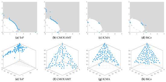
Figure 1.
The final solution sets produced by four representative CMOEAs on the 2-objective LIRCMOP10 problem and the 3-objective C1_DTLZ1 problem.
To bridge these research gaps, this study introduces a weak constraint-Pareto dominance relation that integrates feasibility and objective performance, thereby avoiding the premature elimination of promising infeasible solutions with strong convergence or diversity. Moreover, an angle distance-based diversity maintenance strategy is proposed to enhance diversity while maintaining feasibility within the population. By combining these two mechanisms, we develop the CMOEA-WA algorithm, which demonstrates clear advantages over existing methods.
3. The Proposed CMOEA-WA
This section is organized as follows. We first outline the overall framework of the proposed CMOEA-WA and then provide a detailed discussion of its innovative components.
3.1. Algorithmic Framework of CMOEA-WA
The CMOEA-WA framework Algorithm 1 introduces three complementary archives to balance constraint feasibility, convergence, and diversity throughout the evolutionary process. At initialization, the algorithm generates the main population and establishes the Feasibility-Driven Archive (), Forward-Exploration Archive (), and Diversity-Enhancement Archive (). Each archive is updated independently, focusing on feasible solution preservation, search direction exploration, and diversity maintenance, respectively. In each iteration, parent solutions are selected from the three archives according to their distinct roles, and offspring are generated via genetic operators, enabling coordinated progress toward convergence and diversity in multi-objective optimization.
| Algorithm 1 Framework of CMOEA-WA |
| Input: N (population size), (maximum iterations) |
Output: (Feasibility-Driven Archive)
|
Upon completion, the is returned as the final solution set. By prioritizing feasibility, it ensures that the results both approximate the and satisfy all constraints. Meanwhile, the and reinforce exploration and diversity, mitigating premature convergence and improving solution distribution. Through this collaborative mechanism, CMOEA-WA offers a robust and efficient approach to solving constrained multi-objective optimization problems.
For a clearer representation of the proposed CMOEA-WA, its flowchart is depicted in Figure 2. As shown, the framework is structured around three primary archives: the , , and the . These components are designed to address unconstrained optimization, feasibility-diversity optimization, and constraint-based optimization, respectively, thereby ensuring a comprehensive balance between exploration, diversity preservation, and feasibility maintenance.
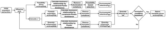
Figure 2.
Framework flowchart of CMOEA-WA.
3.2. Weak Constraint–Pareto Dominance and Angle Distance-Based Diversity Strategy
To clarify the implementation, we provide the formal definition of weak constraint–Pareto dominance and the angle distance-based diversity strategy.
3.2.1. Weak Constraint–Pareto Dominance
Let denote the feasible region of a constrained multi-objective optimization problem (CMOP). The following lemma demonstrates the consistency of the proposed weak constraint–Pareto dominance with the standard Pareto dominance within the feasible region.
Lemma 1
(Consistency over the Feasible Set). If and there exists no feasible solution such that , then is Pareto optimal in .
Proof.
Suppose, to the contrary, that is not Pareto optimal in . Then there exists a feasible solution such that
Since both y and are feasible, we have for all i. According to the definition of weak constraint–Pareto dominance, , which contradicts the assumption. Therefore, must be Pareto optimal. □
Theorem 1
(Fidelity and Asymptotic Optimality of Weak Constraint–Pareto Dominance). Let denote a sequence of solutions generated by an algorithm, satisfying the following:
- (1)
- Each objective function and constraint function is continuous on ;
- (2)
- The aggregate constraint violation is non-increasing, i.e., for any i, for some bounded M;
- (3)
- There exists a convergent subsequence such that , meaning that the limit point is feasible.
If the algorithm updates or archives individuals solely according to the weak constraint–Pareto dominance rule (i.e., any v weakly dominated by another u satisfying is replaced or discarded), then the limit point is a Pareto optimal solution in , or at least a weakly nondominated feasible solution.
From assumptions (1) and (3), continuity ensures that the limit point is feasible. Suppose is not Pareto optimal in ; then there exists such that
By continuity, for sufficiently large k, and become arbitrarily close to and , implying . According to the weak constraint–Pareto dominance rule, such dominated individuals should be replaced in later generations, contradicting the existence of an infinite subsequence converging to . Thus, must be weakly nondominated within ; by Lemma 1, it is Pareto optimal.
The proposed weak constraint–Pareto dominance exhibits several desirable theoretical properties. First, as established in Lemma 1, it is consistent with the standard Pareto dominance when restricted to the feasible set, ensuring that no true Pareto optimal solutions are excluded. Second, Theorem 1 demonstrates its theoretical soundness, showing that under mild continuity and boundedness assumptions, algorithms guided by this dominance relation can asymptotically converge to Pareto-optimal or weakly nondominated feasible solutions. Finally, compared with existing constraint-handling mechanisms such as the constrained domination principle (CDP) and the -constraint method, the proposed dominance relation maintains CDP’s feasible-first property for feasible comparisons while allowing promising partially feasible solutions with superior objective performance to survive. This effectively mitigates CDP’s overemphasis on constraint satisfaction and avoids the parameter sensitivity inherent in -constraint approaches.
3.2.2. Angle Distance-Based Diversity Strategy
For two solutions x and y, the angle distance in the normalized objective space is defined as
where is the reference point. This measure is used to guide selection in the archive to maintain diversity by preferring solutions with larger angles to already selected individuals.
This procedure ensures that only nondominated solutions are retained while preserving diversity across the objective space. The combination of weak constraint–Pareto dominance and angle distance-based diversity strategy allows the algorithm to traverse potentially infeasible regions while maintaining a well-distributed solution set.
3.3. Forward-Exploration Archive
Algorithm 2 illustrates the update process of the . Initially, the FEA is combined with the offspring set to incorporate newly generated solutions and preserve search completeness. The weak constraint–Pareto dominance relations among all solutions are then evaluated, and dominated solutions are discarded. Since only objective values are considered, this step emphasizes objective-space exploration and enables the algorithm to traverse potentially infeasible regions.
If the number of solutions in the archive is less than the sub-population size , random duplication is applied to maintain archive size and prevent diversity loss. Otherwise, the nadir point is computed and, together with the reference point z, used to normalize objective values, thereby mitigating scale differences among objectives. The normalized solutions are subsequently refined using an environmental selection strategy (e.g., NSGA-II, NSGA-III, SPEA2), which eliminates redundancy while preserving representative and diverse individuals. Through this process, the updated FEA is produced to guide the following evolutionary steps.
| Algorithm 2 Update procedure of Forward-Exploration Archive (FEA). |
| Input: (forward-exploration archive), (offspring), (Reference Point), (sub-population size) |
Output: Updated forward-exploration archive
|
3.4. Diversity-Enhancement Archive
To further improve the uniformity and diversity of solutions during the search process, this study incorporates a Diversity-Enhancement Archive Algorithm 3 () update mechanism into the algorithmic framework. This mechanism not only considers feasibility under constraints but also guides the distribution of solutions in the objective space through reference vectors, thereby enhancing the adaptability of the algorithm to complex optimization problems.
| Algorithm 3 Update procedure of Diversity-Enhancement Archive (DEA). |
| Input: (diversity-enhancement archive), (offspring set), (reference point), (number of reference vectors) |
Output: Updated diversity-enhancement archive
|
Specifically, the DEA update procedure first merges the current archive with the offspring population and removes dominated solutions using weak constraint-based Pareto dominance, thereby retaining only the nondominated solutions. On this basis, the nadir point is determined from the feasible solutions; if no feasible solution exists, the solution with the smallest constraint violation is used instead. Subsequently, all objective vectors are normalized using the reference point and the nadir point , eliminating scale differences across objectives.
In the normalized space, a set of reference vectors W is generated, and solutions are assigned to different subspaces according to angular distance. For each reference vector, if its subspace is empty, the solution with the smallest angular distance to the reference vector is selected (regardless of feasibility). If the subspace contains solutions, the solution with the best fitness is chosen and added to the archive. The fitness function is defined as follows:
where denotes the perpendicular distance between solution and reference vector j, represents the constraint violation of solution , and h is a penalty factor. This definition enables the algorithm to prioritize feasibility while maintaining diversity.
In summary, the proposed update mechanism preserves feasible solutions while guiding the population toward a more uniform distribution in the objective space, thereby significantly improving both population diversity and global search performance.
3.5. Feasibility-Driven Archive
The diversity-enhancement archive Algorithm 3 () introduced earlier is mainly designed to improve solution uniformity and distribution. However, when feasible solutions are insufficient, relying solely on DEA may leave the algorithm without effective candidates for optimization. To address this issue, the feasibility-driven archive Algorithm 4 () is introduced with the primary objective of maximizing the preservation and exploitation of feasible solutions. Compared with DEA, FDA places greater emphasis on feasibility and less on diversity, making the two archives complementary within the overall framework.
| Algorithm 4 Update procedure of Feasibility-Driven Archive (FDA). |
| Input: (feasibility-exploitation archive), (offspring set), N (population size), (reference point) |
Output: Updated feasibility-exploitation archive
|
The FDA update procedure can be summarized as follows: first, the current archive is merged with the to form the candidate set S, where dominated solutions are removed using weak constraint–Pareto dominance. If , solutions are randomly duplicated until the population size reaches N, and the archive is returned. When , solutions are sorted in ascending order of constraint violation (), and the number of feasible solutions is counted. If feasible solutions are fewer than N, the top N solutions according to ranking are retained, ensuring that feasibility is maximized.
When feasible solutions are sufficient, all infeasible ones are discarded. The nadir point is then calculated from the feasible solutions, and objective vectors are normalized using both the reference point and . Finally, an environmental selection method (e.g., SPEA2, NSGA-II, or NSGA-III) is applied to select exactly N solutions, balancing convergence and distribution.
In summary, the FDA guarantees feasibility when feasible solutions are scarce and shifts its focus to convergence and distribution once feasible solutions are abundant. Together with the DEA, which maintains diversity, the FDA strengthens the algorithm’s overall ability to solve constrained multi-objective optimization problems.
4. Experimental Studies
All the experiments involved in this section were conducted using the multi-objective evolutionary optimization platform PlatEMO v4.13 [61] under MATLAB. The FEA, DEA, and FDA target distinct aspects of CMO, emphasizing exploration, diversity, and feasibility, respectively. To validate the integrated framework, a series of experiments is conducted on standard benchmark problems. The evaluation considers convergence, diversity, and feasibility preservation, with several state-of-the-art algorithms serving as baselines under identical settings. The results offer a thorough comparison, highlighting the effectiveness and robustness of the proposed approach.
4.1. Experimental Settings
This section presents the experimental setup for evaluating the proposed algorithm, including benchmark problems, performance metrics, comparison algorithms, and parameter configurations.
4.1.1. Benchmark Problems
In this work, the proposed algorithm was evaluated on three widely used CMOP test suites: MW [62], LIR-CMOP [31], C_DTLZ/DC_DTLZ [63], and SDC [1]. The MW suite contains 14 diverse problems derived from real-world CMOPs, capturing various characteristics. LIR-CMOP also includes 14 problems, most of which feature large infeasible regions and relatively few feasible solutions. The C_DTLZ and DC_DTLZ suite comprises 10 problems, with constraints applied to both decision variables and objective functions. Experimental comparisons were conducted on eight complex-constrained test problems (SDC). In all comparison experiments, N denotes the population size (set to 100), M represents the number of objectives, and D indicates the number of decision variables. Detailed configurations for each test problem are listed in the corresponding table.
4.1.2. Performance Indicator
The performance of the proposed algorithm is evaluated using three standard metrics.
- (1)
- Convergence: assessed by Inverted Generational Distance (IGD [47]), which measures how close the obtained solutions are to the true Pareto front.
- (2)
- Diversity: measured by hypervolume (HV [64]), indicating the uniformity of solutions along the Pareto front.
- (3)
- Feasibility: the proportion of feasible solutions in the final population, reflecting the algorithm’s ability to satisfy constraints.
Smaller IGD values indicate stronger convergence to the true Pareto front, while larger HV values represent better solution quality and diversity.
4.1.3. Algorithms Compared
To provide a comprehensive performance assessment of CMOEA-WA, we compare it against seven state-of-the-art constrained multi-objective evolutionary algorithms, including ToP [30], POCEA [65], ICMA [29], BiCo [47], CMOEA_MS [50], CMOCSO [66], CMOEMT [58], IMTCMO [36], and MOEADCMT [67]. To offer a clear comparison of the design characteristics and performance variations among different CMOEAs, Table 1 presents each algorithm’s core mechanisms, constraint handling approaches, strengths, and limitations. The table highlights how these algorithms prioritize feasibility, convergence, and diversity differently, serving as a foundation for the following experimental evaluation and analysis. To ensure fairness in comparison, the benchmark algorithms were configured according to their original settings without any modifications.

Table 1.
Summary and comparison of CMOEAs.
Unlike other benchmark algorithms, CMOEA-WA employs weak constraint–Pareto dominance to identify promising solutions and integrates a diversity-enhancement archive to maintain solution diversity while ensuring feasibility, thereby strengthening its ability to solve constrained multi-objective problems (CMOPs) with complex feasible regions. To guarantee a fair comparison, the parameter settings used in the original publications of the other algorithms are adopted in this study.
4.1.4. Experimental Settings and Supplementary Information
All algorithms are performed using PlatEMO v4.13 [61] within the MATLAB R2021a environment, on a system equipped with an Intel(R) Core(TM) i5-7300HQ CPU @ 2.50 GHz and NVIDIA GeForce GTX 1050 Ti (4 GB) as well as Intel(R) HD Graphics 630 (128 MB) GPUs. Each algorithm is executed independently 20 times on the test problems. For the DAS-CMOP, LIR-CMOP, and MW test suites, the maximum number of fitness evaluations (MaxFEs) is set to .
Meanwhile, the statistical differences between CMOEA-WA and other algorithms are evaluated using the Wilcoxon test at a 0.05 significance level [68]. Gray-shaded cells in the table denote the best results obtained for each test problem, and the symbols +, −, and ≈ indicate that the performance is superior to, inferior to, or comparable with the other algorithms, respectively.
4.2. Experimental Results Analysis
To evaluate CMOEA-WA, a series of experiments were performed. This subsection compares its performance with seven benchmark algorithms across the MW, LIR-CMOP, C_DTLZ, DC_DTLZ, SDC test suites and four real-world problems.
4.2.1. Analysis of the MW Test Suite
As shown in Table 2 and Table 3, CMOEA-WA demonstrates clear superiority on the MW test problems. In the IGD results (Table 2), it achieves the best performance on most instances (highlighted in gray), indicating strong capability in approximating the true Pareto front. Statistical comparisons further show that CMOEA-WA significantly outperforms other algorithms on problems such as MW4, MW5, MW8, MW13, and MW14 while obtaining the best results in ten test cases overall, reinforcing its effectiveness. Regarding HV results (Table 3), CMOEA-WA consistently attains the highest hypervolume values across nearly all problems, highlighting its strength in maintaining both diversity and uniformity of solutions. Compared with the seven competitors, it dominates a large number of problems, with many best results, showing that it not only achieves superior convergence but also ensures well-distributed solution sets.
Table 2.
IGD results (mean ± std) of ten algorithms across the MW test problems.
Table 3.
HV results (mean ± std) of ten algorithms across the MW test problems.
To further illustrate the differences, Figure 3 presents the solution distributions of eight CMOEAs on MW14. In this figure, each light blue dot represents a feasible solution in the decision space, illustrating the distribution of solutions obtained by the eight algorithms. The projection along each axis shows how the solutions spread across the different objectives. It can be observed that ToP, ICMA, CMOCSO, BiCo, POCEA, and IMTCMO fail to converge properly as many solutions do not lie on the PF. Although CMOEA_MS, MOEADCMT, and CMOEMT show improved convergence with more solutions located on the PF, their distributions remain uneven, reflecting insufficient diversity. By contrast, CMOEA-WA places all solutions on the PF with uniform distribution, clearly demonstrating a balanced trade-off between convergence and diversity.
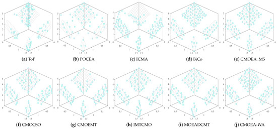
Figure 3.
The final solution sets produced by ten CMOEAs on the 3-objective MW14 problem.
Overall, CMOEA-WA exhibits consistent superiority in both IGD and HV metrics. Combined with the results in Figure 3, it is evident that the algorithm achieves robust performance by effectively balancing convergence and diversity, making it highly competitive on the MW test suite.
4.2.2. Analysis of the LIRCMOP Test Suite
Table 4 and Table 5 present the IGD and HV results of eight algorithms on the LIRCMOP test suite. The results indicate that CMOEA-WA consistently delivers superior performance. For IGD (Table 4), it achieves the best outcomes on most problems (highlighted in gray), demonstrating strong capability in approximating the Pareto front. Statistical comparisons further confirm that CMOEA-WA outperforms its competitors in several cases, reflecting both robustness and convergence efficiency. With respect to HV (Table 5), CMOEA-WA again achieves the highest HV values in the majority of test problems, highlighting its strength in preserving solution diversity and ensuring uniform distribution. While many competing algorithms suffer from poor convergence or limited diversity, CMOEA-WA effectively balances both aspects. This advantage arises from its innovative design, which integrates weak constraint–Pareto dominance for guiding solution selection with a diversity-enhancement archive to maintain feasible and well-distributed solutions.
Table 4.
IGD results (mean ± std) of ten algorithms across the LIRCMOP test problems.
Table 5.
HV results (mean ± std) of ten algorithms across the LIRCMOP test problems.
To summarize, the LIRCMOP experiments reinforce the innovation and effectiveness of CMOEA-WA. By jointly considering feasibility, convergence, and diversity, the algorithm achieves higher accuracy and robustness than existing approaches in solving complex CMOPs.
4.2.3. Analysis of the C_DTLZ and DC_DTLZ Test Suite
The results in Table 6 and Table 7 highlight the clear advantages of CMOEA-WA in tackling complex constrained multi-objective problems. For IGD (Table 6), CMOEA-WA consistently achieves the best or near-best outcomes (marked in gray) across most test instances, reflecting its strong convergence ability toward the true Pareto front. Statistical analysis further indicates that it surpasses many competitors in several cases, demonstrating both robustness and stability. In terms of HV (Table 7), CMOEA-WA attains the highest hypervolume values in almost all problems, emphasizing its superior capacity to preserve diversity and ensure uniformly distributed solutions. In contrast, other algorithms often suffer from weak convergence in C_DTLZ or fail to provide well-distributed solutions in the disconnected feasible regions of DC_DTLZ, whereas CMOEA-WA effectively balances feasibility, convergence, and diversity.
Table 6.
IGD results (mean ± std) of ten algorithms across the C_DTLZ and DC_DTLZ test problems.
Table 7.
HV results (mean ± std) of ten algorithms across the C_DTLZ and DC_DTLZ test problems.
These strengths arise from the algorithm’s innovative framework. By embedding weak constraint–Pareto dominance into its selection process, CMOEA-WA favors feasible solutions while maintaining pressure toward the Pareto front. At the same time, the diversity-enhancement archive ensures evenly spread solutions even under highly complex or disconnected feasible regions. To summarize, the experiments on C_DTLZ and DC_DTLZ demonstrate that CMOEA-WA not only delivers superior convergence and diversity but also maintains strong competitiveness in solving challenging CMOPs, confirming the effectiveness of its novel design.
4.2.4. Analysis of the SDC Test Suite
To further evaluate the performance of the algorithms under more complex constraints, we conducted a comparative analysis of ten algorithms on the SDC test problems. According to the IGD results shown in Table 8, CMOEA-WA demonstrates the best overall performance and stability on the SDC test problems. Among the eight test problems, CMOEA-WA achieves the best IGD values on six problems (SDC1, SDC2, SDC4, SDC5, SDC7, and SDC8), with relatively small standard deviations, indicating good reliability. For SDC3 and SDC6, CMOCSO and IMTCMO perform best, respectively; however, IMTCMO exhibits NaN or extreme IGD values in other problems, indicating lower stability overall. Statistical significance analysis shows that CMOEA-WA is significantly superior to most comparison algorithms on the majority of problems, while other algorithms demonstrate unstable performance with large standard deviations or very high IGD values. In summary, CMOEA-WA not only excels in approximating the Pareto front but also exhibits outstanding stability and reliability, confirming its superior overall performance on the SDC problems. Based on the HV results shown in Table 9, CMOEA-WA demonstrates overall superior performance and stability on the SDC test problems. Although HV values are generally close to zero for most problems, reflecting the high difficulty of these problems, CMOEA-WA still achieves significantly higher HV values on SDC2, SDC7, and SDC8, with moderate standard deviations, indicating good reliability. Some algorithms, such as ICMA and CMOCSO, occasionally perform better on individual problems (e.g., SDC1 and SDC3), but their overall stability is insufficient. For SDC4–SDC6, all algorithms attain HV values of zero, suggesting that these problems are highly challenging for existing methods. Statistical significance analysis further shows that CMOEA-WA is significantly superior or comparable to most algorithms, with no cases of inferior performance. In summary, CMOEA-WA not only approximates the true Pareto front effectively in terms of IGD but also covers a larger portion of the front in terms of HV, demonstrating its comprehensive advantage in both performance and stability.
Table 8.
IGD results (mean ± std) of ten algorithms across the SDC test problems.
Table 9.
HV results (mean ± std) of ten algorithms across the SDC test problems.
A closer inspection reveals that the innovation of CMOEA-WA lies in its multi-strategy cooperative mechanism and dynamic weight adjustment, enabling it to balance feasibility, convergence, and diversity simultaneously. Notably, even on extremely challenging problems like SDC6 and SDC8, CMOEA-WA maintains superior performance while other algorithms experience significant degradation. This demonstrates that CMOEA-WA not only improves robustness in solving complex constrained problems but also ensures a well-distributed solution set.
4.3. Scalability and Computational Cost
In this study, to evaluate the computational overhead and scalability of CMOEA-WA, we analyzed the main operations in each generation. Assuming a population size of N, objective dimensionality M, and archive size K, the main computational costs of CMOEA-WA arise from three components: the weak constraint–Pareto dominance calculation with complexity , the angle-based diversity maintenance with complexity , and the management of multiple archives with complexity . Overall, the per-generation time complexity of CMOEA-WA can be approximated as , with angle-based calculations dominating as the number of objectives increases.
For a clearer comparison, we also considered two commonly used baseline algorithms: NSGA-II and BiCo. NSGA-II has a per-generation complexity of due to nondominated sorting, while BiCo employs a co-evolutionary strategy with a per-generation complexity roughly , depending on archive updates. Compared with these baselines, CMOEA-WA introduces additional computational overhead primarily from angle-based diversity maintenance and multiple-archive management, but this overhead grows moderately with population size and the number of objectives.
Based on runtime, function evaluation counts and performance on standard CMOP benchmark problems such as MW, LIRCMOP, C-DTLZ/DC-DTLZ, and SDC (Table 2, Table 4, Table 6 and Table 8), it is evident that CMOEA-WA maintains high-quality solutions and diversity while keeping computational overhead within a reasonable range. As the number of objectives increases in these benchmarks, angle-based diversity maintenance gradually becomes the dominant factor, consistent with theoretical complexity analysis. Nevertheless, CMOEA-WA remains computationally feasible, and the additional overhead is justified by the improved solution quality and diversity.
Overall, the computational overhead of CMOEA-WA scales roughly quadratically with population size and linearly with the number of objectives. Compared with NSGA-II and BiCo, the additional time cost is moderate, while the benefits in maintaining solution quality and diversity are clearly demonstrated on the considered benchmark problems. Therefore, CMOEA-WA achieves a favorable trade-off between computational cost and performance, showing good scalability in practice.
As shown in Table 10, CMOEA-WA demonstrates both high computational efficiency and superior solution quality across all test problem sets (MW, LIRCMOP, SDC, C-DTLZ). Its average runtime per generation is comparable to or lower than most baseline algorithms while consistently achieving the best or near-best IGD and HV values. This indicates that the weighted archiving mechanism and multi-strategy cooperative optimization effectively balance convergence, diversity, and efficiency. Overall, CMOEA-WA achieves an excellent trade-off between performance and runtime, making it highly suitable for large-scale, constrained multi-objective optimization problems.
Table 10.
Runtime and function evaluations (FEs) of CMOEA-WA and baseline algorithms on selected test problems (average ± std).
4.4. Performance Analysis of CMOEA-WA
From the IGD and HV boxplots Figure 4 (with logarithmic scale on the y-axis and 95% confidence intervals), it is evident that CMOEA-WA demonstrates significant advantages across various constrained multi-objective optimization problems. Its IGD means are generally the lowest or near the lowest, with relatively short boxes and whiskers, indicating that the algorithm approximates the true Pareto front both accurately and stably. The HV means are high with small variability, reflecting enhanced coverage of the Pareto front and effectively avoiding the large performance fluctuations observed in other algorithms. Statistical significance tests further confirm that these performance improvements are not coincidental but result from the fundamentally improved solution generation and selection mechanisms.
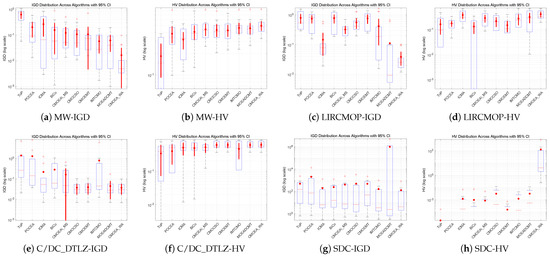
Figure 4.
The IGD and HV boxplots of the performances of each algorithm.
CMOEA-WA also exhibits excellent convergence robustness and solution set distribution stability. The narrow confidence intervals across subplots indicate minimal performance fluctuations over multiple independent runs, demonstrating the effectiveness of the weighted archiving mechanism in balancing convergence speed and population diversity. This mechanism prevents the algorithm from becoming trapped in local optima, enabling it to consistently produce high-quality and uniformly distributed Pareto-approximate solutions across different problem types and scales, such as MW, SDC, and C/DC_DTLZ.
The advantages of CMOEA-WA are even more pronounced when handling complex constrained problems. Particularly for LIRCMOP and C/DC_DTLZ problems with complex constraints and irregular Pareto fronts, the superiority of mean performance and separation of confidence intervals are clearly observed, highlighting the effectiveness of the innovative mechanisms—weak constraint–Pareto dominance and multi-strategy collaborative optimization. These mechanisms not only enhance convergence accuracy and coverage but also improve stability and robustness, effectively reducing stagnation in local optima. Overall, CMOEA-WA outperforms other mainstream constrained multi-objective optimization algorithms in terms of accuracy, stability, and adaptability.
4.5. Analysis of Real-World Case Problems
From Table 11, CMOEA-WA demonstrates consistently strong performance on real-world engineering problems. Specifically, it attains the highest HV values (highlighted in gray) across all four test problems (DEB, CTP, CSID, and FBPT), indicating its effective balance between convergence and solution diversity under complex multi-objective and constrained scenarios. In comparison, competing algorithms often suffer from inadequate convergence or non-uniform solution distributions when addressing these challenging, highly constrained problems.
Table 11.
HV results (mean ± std) of ten algorithms across the real-world case problems.
This superior performance reflects the practical applicability of CMOEA-WA. In real engineering scenarios, where constraints can be tight and objectives conflicting, the integration of weak constraint–Pareto dominance ensures that feasible and informative solutions are preserved while guiding the population toward the true Pareto front. Moreover, the diversity-enhancement archive promotes broad coverage and uniform solution distribution, which is crucial for providing multiple viable options in decision-making processes.
In summary, the results from real-world case studies confirm not only the robustness but also the practical utility of CMOEA-WA. By maintaining high-quality, well-distributed solution sets in multi-constrained engineering optimization problems, CMOEA-WA proves to be highly suitable for real-world applications, effectively bridging the gap between theoretical benchmark performance and practical engineering needs.
4.6. Ablation Study on MW Test Problems
Based on the IGD and HV results of the three variants and CMOEA-WA (CMOEACD), the quantitative analysis can be summarized as follows:
From the Table 12 IGD results, it is evident that CMOEA-WA achieves the best performance across the majority of the 14 MW test problems, with consistently small standard deviations, indicating high accuracy and stability. Among the variants, CMOEA-WA1 (without the three cooperative external archives mechanism) performs comparably to CMOEA-WA on a few problems (e.g., MW1, MW4, MW7, MW8, MW12), but generally shows higher IGD values. CMOEA-WA2 (without weak constraint–Pareto dominance) exhibits significantly worse IGD on most problems, highlighting the critical role of the weakly cooperative dominance in guiding the search toward the true Pareto front. CMOEA-WA3 (angle distance-based diversity maintenance strategy ) also suffers from increased IGD on several problems, particularly MW2, MW3, MW5, and MW6, demonstrating the importance of angle-based selection in maintaining solution diversity and uniformity.
Table 12.
IGD results (mean ± std) of three variants and CMOEA-WA the MW case problems.
The Table 13 HV results further confirm the superiority of CMOEA-WA, which achieves the highest HV values on nearly all problems, indicating the largest coverage of the Pareto front and strong stability. Among the variants, CMOEA-WA1 occasionally approaches the performance of CMOEA-WA on certain problems (e.g., MW12) but overall shows lower HV. CMOEA-WA2 and CMOEA-WA3 consistently attain lower HV values, with some NaN or zero values, indicating that removing the weakly cooperative Pareto dominance or angle-based selection reduces the algorithm’s ability to maintain a well-distributed solution set. These results highlight that CMOEA-WA’s mechanisms significantly enhance the coverage and distribution of solutions.
Table 13.
HV results (mean ± std) of three variants and CMOEA-WA the MW case problems.
The comparison demonstrates the innovative contributions of CMOEA-WA. The three cooperative external archives mechanism enhances exploration and maintains diversity across different regions of the Pareto front. The weak constraint–Pareto dominance effectively guides convergence toward the true Pareto front, reducing IGD. The angle distance-based diversity maintenance strategy ensures a uniform distribution of solutions, improving HV. By integrating these three mechanisms, CMOEA-WA achieves superior convergence, better solution distribution, and high stability across the MW test problems, clearly demonstrating its comprehensive advantage and the effectiveness of its design innovations.
5. Conclusions
This paper introduces CMOEA-WA, a constrained multi-objective evolutionary algorithm designed to overcome the tendency of existing approaches to overemphasize feasibility while discarding informative infeasible solutions. The proposed method incorporates three complementary mechanisms: (i) a weak constraint–Pareto dominance relation that jointly considers feasibility and objective quality, (ii) an angle distance-based strategy that preserves solution diversity through uniform distribution, and (iii) three cooperative external archives dedicated to unconstrained, feasibility-based, and fully constrained optimization. By combining these components, CMOEA-WA effectively retains promising solutions, sustains population diversity, and enhances overall search efficiency.
Extensive experiments on benchmark suites and real-world engineering problems demonstrate that CMOEA-WA consistently surpasses state-of-the-art algorithms in terms of feasibility, convergence, and diversity. These results verify both the robustness and the practical value of the proposed framework, underscoring its suitability for complex constrained multi-objective problems.
Future work will focus on several directions: extending CMOEA-WA to dynamic and large-scale optimization problems, addressing many-objective scenarios, and exploring its integration with machine learning techniques to enhance adaptive constraint handling and improve performance in real-world decision-making environments. These avenues aim to further strengthen the algorithm’s adaptability, scalability, and practical applicability.
Author Contributions
Conceptualization, J.G. and Y.S.; Methodology, Y.S.; Software, Y.S.; Validation, Y.S. and J.G.; Formal analysis, Y.S.; Investigation, Y.S.; Resources, J.G.; Data curation, J.G. and Y.S.; Writing—original draft preparation, J.G. and Y.S.; Writing—review and editing, J.G. and Y.S.; Visualization, Y.S.; Supervision, J.G. and Y.S.; Project administration, J.G.; Funding acquisition, J.G. All authors have read and agreed to the published version of the manuscript.
Funding
This research was funded by Science Foundation of Hubei Province of China (grant number: No.2022CFB935). The APC was funded by Wuhan Second Ship Design and Research Institute.
Data Availability Statement
All experimental data used in this study were obtained from the PlatEMO 4.13 platform, which provides publicly available benchmark test sets (MW, LIRCMOP, C_DTLZ/DC_DTLZ and SDC). The source code can be accessed at https://github.com/BIMK/PlatEMO (accessed on 2 November 2025) and https://github.com/MrFENGXINGYU/CMOEA-WA (accessed on 4 November 2025).
Conflicts of Interest
The authors declare no conflicts of interest.
References
- Hao, L.; Peng, W.; Liu, J.; Zhang, W.; Li, Y.; Qin, K. Competition-based two-stage evolutionary algorithm for constrained multi-objective optimization. Math. Comput. Simul. 2025, 230, 207–226. [Google Scholar] [CrossRef]
- Cao, J.; Yan, Z.; Chen, Z.; Zhang, J. A Pareto front estimation-based constrained multi-objective evolutionary algorithm. Appl. Intell. 2023, 53, 10380–10416. [Google Scholar] [CrossRef]
- Yang, Y.; Liu, J.; Tan, S. A constrained multi-objective evolutionary algorithm based on decomposition and dynamic constraint-handling mechanism. Appl. Soft Comput. 2020, 89, 106104. [Google Scholar] [CrossRef]
- Zuo, X.; Chen, C.; Tan, W.; Zhou, M. Vehicle scheduling of an urban bus line via an improved multiobjective genetic algorithm. IEEE Trans. Intell. Transp. Syst. 2014, 16, 1030–1041. [Google Scholar] [CrossRef]
- Ma, L.; Li, N.; Guo, Y.; Wang, X.; Yang, S.; Huang, M.; Zhang, H. Learning to optimize: Reference vector reinforcement learning adaption to constrained many-objective optimization of industrial copper burdening system. IEEE Trans. Cybern. 2021, 52, 12698–12711. [Google Scholar] [CrossRef]
- Liu, D.; Shan, X.; Zhao, B.; Luo, B.; Wei, Q. Adaptive Dynamic Programming for Control: A Survey and Recent Advances. IEEE Trans. Syst. Man Cybern. Syst. 2020, 61, 142–160. [Google Scholar] [CrossRef]
- Jan, M.A.; Khanum, R.A. A study of two penalty-parameterless constraint handling techniques in the framework of MOEA/D. Appl. Soft Comput. 2013, 13, 128–148. [Google Scholar] [CrossRef]
- Liu, J.; Wang, Y.; Fan, N.; Wei, S.; Tong, W. A convergence-diversity balanced fitness evaluation mechanism for decomposition-based many-objective optimization algorithm. Integr. Comput.-Aided Eng. 2019, 26, 159–184. [Google Scholar] [CrossRef]
- Zhang, S.; Yang, F.; Yan, C.; Zhou, D.; Zeng, X. An efficient batch-constrained bayesian optimization approach for analog circuit synthesis via multiobjective acquisition ensemble. IEEE Trans. Comput.-Aided Des. Integr. Circuits Syst. 2021, 41, 1–14. [Google Scholar] [CrossRef]
- Liang, J.; Ban, X.; Yu, K.; Qu, B.; Qiao, K.; Yue, C.; Chen, K.; Tan, K.C. A survey on evolutionary constrained multiobjective optimization. IEEE Trans. Evol. Comput. 2022, 27, 201–221. [Google Scholar] [CrossRef]
- Ming, F.; Gong, W.; Zhen, H.; Li, S.; Wang, L.; Liao, Z. A simple two-stage evolutionary algorithm for constrained multi-objective optimization. Knowl.-Based Syst. 2021, 228, 107263. [Google Scholar] [CrossRef]
- Woldesenbet, Y.G.; Yen, G.G.; Tessema, B.G. Constraint handling in multiobjective evolutionary optimization. IEEE Trans. Evol. Comput. 2009, 13, 514–525. [Google Scholar] [CrossRef]
- Ray, T.; Tai, K.; Seow, K.C. Multiobjective design optimization by an evolutionary algorithm. Eng. Optim. 2001, 33, 399–424. [Google Scholar] [CrossRef]
- Fan, Z.; Li, W.; Cai, X.; Li, H.; Wei, C.; Zhang, Q.; Deb, K.; Goodman, E. Push and pull search for solving constrained multi-objective optimization problems. Swarm Evol. Comput. 2019, 44, 665–679. [Google Scholar] [CrossRef]
- Bao, Q.; Wang, M.; Dai, G.; Chen, X.; Song, Z.; Li, S. An archive-based two-stage evolutionary algorithm for constrained multi-objective optimization problems. Swarm Evol. Comput. 2022, 75, 101161. [Google Scholar] [CrossRef]
- Deb, K.; Pratap, A.; Agarwal, S.; Meyarivan, T. A fast and elitist multiobjective genetic algorithm: NSGA-II. IEEE Trans. Evol. Comput. 2002, 6, 182–197. [Google Scholar] [CrossRef]
- Wang, P.; Ma, Y.; Wang, M. A dynamic multi-objective optimization evolutionary algorithm based on particle swarm prediction strategy and prediction adjustment strategy. Swarm Evol. Comput. 2022, 75, 101164. [Google Scholar] [CrossRef]
- Ruan, G.; Yu, G.; Zheng, J.; Zou, J.; Yang, S. The effect of diversity maintenance on prediction in dynamic multi-objective optimization. Appl. Soft Comput. 2017, 58, 631–647. [Google Scholar] [CrossRef]
- Liu, S.; Lin, Q.; Li, Q.; Tan, K.C. A comprehensive competitive swarm optimizer for large-scale multiobjective optimization. IEEE Trans. Syst. Man Cybern. Syst. 2021, 52, 5829–5842. [Google Scholar] [CrossRef]
- He, C.; Cheng, R.; Yazdani, D. Adaptive offspring generation for evolutionary large-scale multiobjective optimization. IEEE Trans. Syst. Man Cybern. Syst. 2020, 52, 786–798. [Google Scholar] [CrossRef]
- Bader, J.; Zitzler, E. HypE: An algorithm for fast hypervolume-based many-objective optimization. Evol. Comput. 2011, 19, 45–76. [Google Scholar] [CrossRef] [PubMed]
- Coello, C.A.C. Theoretical and numerical constraint-handling techniques used with evolutionary algorithms: A survey of the state of the art. Comput. Methods Appl. Mech. Eng. 2002, 191, 1245–1287. [Google Scholar] [CrossRef]
- Wang, P.; Xiao, H.; Han, X.; Yang, F.; Li, L. A coevolutionary algorithm based on reference line guided archive for constrained multiobjective optimization. Appl. Soft Comput. 2023, 142, 110169. [Google Scholar] [CrossRef]
- Zitzler, E.; Laumanns, M.; Thiele, L. SPEA2: Improving the strength Pareto evolutionary algorithm. TIK Rep. 2001, 103, 95–100. [Google Scholar]
- Zhang, Q.; Li, H. MOEA/D: A multiobjective evolutionary algorithm based on decomposition. IEEE Trans. Evol. Comput. 2007, 11, 712–731. [Google Scholar] [CrossRef]
- Runarsson, T.P.; Yao, X. Stochastic ranking for constrained evolutionary optimization. IEEE Trans. Evol. Comput. 2000, 4, 284–294. [Google Scholar] [CrossRef]
- Ming, M.; Wang, R.; Ishibuchi, H.; Zhang, T. A Novel Dual-Stage Dual-Population Evolutionary Algorithm for Constrained Multiobjective Optimization. IEEE Trans. Evol. Comput. 2021, 26, 1129–1143. [Google Scholar] [CrossRef]
- Qin, C.; Ming, F.; Gong, W.; Gu, Q. Constrained multi-objective optimization via two archives assisted push–pull evolutionary algorithm. Swarm Evol. Comput. 2022, 75, 101178. [Google Scholar] [CrossRef]
- Yuan, J.; Liu, H.L.; Ong, Y.S.; He, Z. Indicator-based evolutionary algorithm for solving constrained multiobjective optimization problems. IEEE Trans. Evol. Comput. 2021, 26, 379–391. [Google Scholar] [CrossRef]
- Liu, Z.Z.; Wang, Y. Handling constrained multiobjective optimization problems with constraints in both the decision and objective spaces. IEEE Trans. Evol. Comput. 2019, 23, 870–884. [Google Scholar] [CrossRef]
- Fan, Z.; Li, W.; Cai, X.; Huang, H.; Fang, Y.; You, Y.; Mo, J.; Wei, C.; Goodman, E. An improved epsilon constraint-handling method in MOEA/D for CMOPs with large infeasible regions. arXiv 2017, arXiv:1707.08767. [Google Scholar] [CrossRef]
- Tian, Y.; Zhang, T.; Xiao, J.; Zhang, X.; Jin, Y. A coevolutionary framework for constrained multiobjective optimization problems. IEEE Trans. Evol. Comput. 2020, 25, 102–116. [Google Scholar] [CrossRef]
- Tian, Y.; Zhang, Y.; Su, Y.; Zhang, X.; Tan, K.C.; Jin, Y. Balancing objective optimization and constraint satisfaction in constrained evolutionary multiobjective optimization. IEEE Trans. Cybern. 2021, 52, 9559–9572. [Google Scholar] [CrossRef] [PubMed]
- Li, K.; Chen, R.; Fu, G.; Yao, X. Two-archive evolutionary algorithm for constrained multiobjective optimization. IEEE Trans. Evol. Comput. 2018, 23, 303–315. [Google Scholar] [CrossRef]
- Zhu, Q.; Zhang, Q.; Lin, Q. A constrained multiobjective evolutionary algorithm with detect-and-escape strategy. IEEE Trans. Evol. Comput. 2020, 24, 938–947. [Google Scholar] [CrossRef]
- Qiao, K.; Liang, J.; Yu, K.; Yue, C.; Lin, H.; Zhang, D.; Qu, B. Evolutionary constrained multiobjective optimization: Scalable high-dimensional constraint benchmarks and algorithm. IEEE Trans. Evol. Comput. 2023, 28, 965–979. [Google Scholar] [CrossRef]
- Akherati, H.; Beyramzad, J.; Khiyabani, S.S.; Shariatinezhad, A.; Eskandari, E. Finite-time stable model free sliding mode attitude controller/observer design for uncertain space systems based on time delay estimation. Adv. Space Res. 2025, 76, 3573–3594. [Google Scholar] [CrossRef]
- Schieber, B.; Vahidi, S. Approximating Connected Maximum Cuts via Local Search. In Proceedings of the 31st Annual European Symposium on Algorithms (ESA 2023), Amsterdam, The Netherlands, 4–6 September 2023; Volume 274, pp. 93:1–93:17. [Google Scholar] [CrossRef]
- Jain, H.; Deb, K. An evolutionary many-objective optimization algorithm using reference-point based nondominated sorting approach, part II: Handling constraints and extending to an adaptive approach. IEEE Trans. Evol. Comput. 2013, 18, 602–622. [Google Scholar] [CrossRef]
- Fan, Z.; Li, W.; Cai, X.; Hu, K.; Lin, H.; Li, H. Angle-based constrained dominance principle in MOEA/D for constrained multi-objective optimization problems. In Proceedings of the 2016 IEEE Congress on Evolutionary Computation (CEC), Vancouver, BC, Canada, 24–29 July 2016; pp. 460–467. [Google Scholar]
- Fan, Z.; Fang, Y.; Li, W.; Cai, X.; Wei, C.; Goodman, E. MOEA/D with angle-based constrained dominance principle for constrained multi-objective optimization problems. Appl. Soft Comput. 2019, 74, 621–633. [Google Scholar] [CrossRef]
- Ma, H.; Wei, H.; Tian, Y.; Cheng, R.; Zhang, X. A multi-stage evolutionary algorithm for multi-objective optimization with complex constraints. Inf. Sci. 2021, 560, 68–91. [Google Scholar] [CrossRef]
- Yang, Y.; Liu, J.; Tan, S.; Wang, H. A multi-objective differential evolutionary algorithm for constrained multi-objective optimization problems with low feasible ratio. Appl. Soft Comput. 2019, 80, 42–56. [Google Scholar] [CrossRef]
- Liu, Z.Z.; Qin, Y.; Song, W.; Zhang, J.; Li, K. Multiobjective-based constraint-handling technique for evolutionary constrained multiobjective optimization: A new perspective. IEEE Trans. Evol. Comput. 2022, 27, 1370–1384. [Google Scholar] [CrossRef]
- Ning, W.; Guo, B.; Yan, Y.; Wu, X.; Wu, J.; Zhao, D. Constrained multi-objective optimization using constrained non-dominated sorting combined with an improved hybrid multi-objective evolutionary algorithm. Eng. Optim. 2017, 49, 1645–1664. [Google Scholar] [CrossRef]
- Wang, J.; Li, Y.; Zhang, Q.; Zhang, Z.; Gao, S. Cooperative multiobjective evolutionary algorithm with propulsive population for constrained multiobjective optimization. IEEE Trans. Syst. Man Cybern. Syst. 2021, 52, 3476–3491. [Google Scholar] [CrossRef]
- Liu, Z.Z.; Wang, B.C.; Tang, K. Handling constrained multiobjective optimization problems via bidirectional coevolution. IEEE Trans. Cybern. 2021, 52, 10163–10176. [Google Scholar] [CrossRef]
- Fan, Z.; Wang, Z.; Li, W.; Yuan, Y.; You, Y.; Yang, Z.; Sun, F.; Ruan, J. Push and pull search embedded in an M2M framework for solving constrained multi-objective optimization problems. Swarm Evol. Comput. 2020, 54, 100651. [Google Scholar] [CrossRef]
- Sun, R.; Zou, J.; Liu, Y.; Yang, S.; Zheng, J. A multistage algorithm for solving multiobjective optimization problems with multiconstraints. IEEE Trans. Evol. Comput. 2022, 27, 1207–1219. [Google Scholar] [CrossRef]
- Tang, H.; Yu, F.; Zou, J.; Yang, S.; Zheng, J. A constrained multi-objective evolutionary strategy based on population state detection. Swarm Evol. Comput. 2022, 68, 100978. [Google Scholar] [CrossRef]
- Xia, M.; Chong, Q.; Dong, M. A constrained multi-objective evolutionary algorithm with two-stage resources allocation. Swarm Evol. Comput. 2023, 79, 101313. [Google Scholar] [CrossRef]
- Zou, J.; Sun, R.; Liu, Y.; Hu, Y.; Yang, S.; Zheng, J.; Li, K. A multipopulation evolutionary algorithm using new cooperative mechanism for solving multiobjective problems with multiconstraint. IEEE Trans. Evol. Comput. 2023, 28, 267–280. [Google Scholar] [CrossRef]
- Liang, J.; Lin, H.; Yue, C.; Yu, K.; Guo, Y.; Qiao, K. Multiobjective differential evolution with speciation for constrained multimodal multiobjective optimization. IEEE Trans. Evol. Comput. 2022, 27, 1115–1129. [Google Scholar] [CrossRef]
- Yang, K.; Zheng, J.; Zou, J.; Yu, F.; Yang, S. A dual-population evolutionary algorithm based on adaptive constraint strength for constrained multi-objective optimization. Swarm Evol. Comput. 2023, 77, 101247. [Google Scholar] [CrossRef]
- Dong, J.; Gong, W.; Ming, F.; Wang, L. A two-stage evolutionary algorithm based on three indicators for constrained multi-objective optimization. Expert Syst. Appl. 2022, 195, 116499. [Google Scholar] [CrossRef]
- Zhou, Y.; Zhu, M.; Wang, J.; Zhang, Z.; Xiang, Y.; Zhang, J. Tri-goal evolution framework for constrained many-objective optimization. IEEE Trans. Syst. Man Cybern. Syst. 2018, 50, 3086–3099. [Google Scholar] [CrossRef]
- Ma, Z.; Wang, Y.; Song, W. A new fitness function with two rankings for evolutionary constrained multiobjective optimization. IEEE Trans. Syst. Man Cybern. Syst. 2019, 51, 5005–5016. [Google Scholar] [CrossRef]
- Ming, F.; Gong, W.; Wang, L.; Gao, L. Constrained multiobjective optimization via multitasking and knowledge transfer. IEEE Trans. Evol. Comput. 2022, 28, 77–89. [Google Scholar] [CrossRef]
- Liang, J.; Qiao, K.; Yu, K.; Qu, B.; Yue, C.; Guo, W.; Wang, L. Utilizing the relationship between unconstrained and constrained pareto fronts for constrained multiobjective optimization. IEEE Trans. Cybern. 2022, 53, 3873–3886. [Google Scholar] [CrossRef]
- Zhang, Y.; Tian, Y.; Jiang, H.; Zhang, X.; Jin, Y. Design and analysis of helper-problem-assisted evolutionary algorithm for constrained multiobjective optimization. Inf. Sci. 2023, 648, 119547. [Google Scholar] [CrossRef]
- Tian, Y.; Cheng, R.; Zhang, X.; Jin, Y. PlatEMO: A MATLAB platform for evolutionary multi-objective optimization [educational forum]. IEEE Comput. Intell. Mag. 2017, 12, 73–87. [Google Scholar] [CrossRef]
- Sun, Y.; Yen, G.G.; Yi, Z. IGD indicator-based evolutionary algorithm for many-objective optimization problems. IEEE Trans. Evol. Comput. 2018, 23, 173–187. [Google Scholar] [CrossRef]
- Deb, K.; Agrawal, R.B. Simulated binary crossover for continuous search space. Complex Syst. 1995, 9, 115–148. [Google Scholar]
- Deb, K.; Goyal, M. A combined genetic adaptive search (GeneAS) for engineering design. Comput. Sci. Inform. 1996, 26, 30–45. [Google Scholar]
- He, C.; Cheng, R.; Tian, Y.; Zhang, X.; Tan, K.C.; Jin, Y. Paired Offspring Generation for Constrained Large-Scale Multiobjective Optimization. IEEE Trans. Evol. Comput. 2021, 25, 448–462. [Google Scholar] [CrossRef]
- Ming, F.; Gong, W.; Li, D.; Wang, L.; Gao, L. A competitive and cooperative swarm optimizer for constrained multiobjective optimization problems. IEEE Trans. Evol. Comput. 2022, 27, 1313–1326. [Google Scholar] [CrossRef]
- Feng, X.; Dang, Q.; Gao, X.; Wu, Y.; Zheng, L. A collaborative competition multitasking framework for constrained multi-objective optimization. Appl. Soft Comput. 2025, 185, 113900. [Google Scholar] [CrossRef]
- Wilcoxon, F. Some rapid approximate statistical procedures. Ann. N. Y. Acad. Sci. 1950, 52, 808–814. [Google Scholar] [CrossRef]
Disclaimer/Publisher’s Note: The statements, opinions and data contained in all publications are solely those of the individual author(s) and contributor(s) and not of MDPI and/or the editor(s). MDPI and/or the editor(s) disclaim responsibility for any injury to people or property resulting from any ideas, methods, instructions or products referred to in the content. |
© 2025 by the authors. Licensee MDPI, Basel, Switzerland. This article is an open access article distributed under the terms and conditions of the Creative Commons Attribution (CC BY) license (https://creativecommons.org/licenses/by/4.0/).