1. Introduction
Industrial power systems are increasingly facing problems related to voltage stability, current harmonic distortions, and generally deteriorating power quality. This issue is mainly due to nonlinear electrical loads, constantly changing operating conditions, and increasing demand for energy efficiency. This condition is especially true for high-power industrial consumers such as metallurgical plants, where electric arc furnaces, ladle furnaces, and hot rolling mills operate. All of these loads are nonlinear and use high-power electrical drives with rapidly fluctuating and transient loads that produce significant harmonic distortions [
1,
2].
Total harmonic distortion (THD) is a key measure of power quality, influencing equipment reliability, energy efficiency, and compliance with international standards [
3,
4]. Passive filters and capacitor banks for reactive power compensation are two methods that have been the focus of several studies aimed at reducing harmonic distortion [
5,
6]. Although these systems function successfully when the load is constant or predictable, they fail when dealing with the frequent and unexpected changes in operating circumstances that are typical of modern industrial settings, like steel rolling mills. In light of this weakness, it is clear that better prediction and control systems are required to detect THD changes before they cause serious issues [
7]. Recently, deep learning (DL) and artificial intelligence (AI) have gained recognition as powerful tools for simulating dynamic and nonlinear processes in power grids. For time series forecasting problems, sequential architectures like LSTM, Bidirectional LSTM (BiLSTM), and Gated Recurrent Units (GRU) have shown promise [
8,
9]. This is due to their ability to accurately capture non-stationary dynamics and long-term temporal dependencies. At the same time, Convolutional Neural Networks (CNN) and deep hybrid models have been successfully applied to extract high-level spatial and temporal features from multidimensional power data, improving both accuracy and generalization in complex industrial scenarios [
7]. More recently, attention-based architectures and transformation networks have been shown to improve forecast accuracy by dynamically weighing temporal relationships, thereby capturing context-dependent patterns in power quality signals [
8,
10].
Building on this research, this paper investigates the measurement-based prediction of Total Harmonic Distortion (THD) in a power system for an industrial rolling mill operating in different configurations—both with and without reactive power compensation. The paper compares the prediction performance of several deep neural architectures in three prediction methods (classical, autoregressive, and multi-step). By analyzing the advantages and limitations of each model, the study presents the potential of modern hybrid and attention-based networks for improving predictive monitoring and resilient operation in industrial power systems.
The present study uses real data measured in the electrical network of a hot rolling mill, thus providing an authentic experimental basis for evaluating the behavior of a reactive power compensation system. Using this real data, the paper presents an extensive comparative analysis of the performances obtained by eight modern deep neural architectures (including various combinations of RNN/LSTM/GRU and hybrid models), evaluated within three distinct forecasting methods: (i) classical direct forecasting (one stage ahead); (ii) iterative autoregressive forecasting (using the model outputs as input for the next steps); and (iii) multi-step forecasting over an extended time horizon. Experimental results highlight that the CNN–GRU–LSTM hybrid architecture proposed in this study is the only model among those tested that manages to maintain a positive coefficient of determination (R2) under the difficult conditions of multi-step forecasting, demonstrating a superior long-term generalization capacity. The study also comparatively evaluates the accuracy of the forecasting models in two operating regimes, highlighting how the compensation regime influences the THD signal variability and the difficulty of the prediction task. By combining these innovative elements, the work provides useful information both on the evaluation of the efficiency of reactive compensation and on the selection of the optimal neural architecture for applications of this type.
4. THD Forecasting Using Deep Learning Models
4.1. Motivation and Modeling Strategy
Accurate prediction of total harmonic distortion (THD) is necessary for real-time monitoring and predictive control of power quality in factories like hot rolling mills. Given the temporal dynamics of THD fluctuations caused by load variations, nonlinear equipment, and reactive power flows, deep learning models with temporal processing abilities are suitable. Several neural network topologies were designed and tested for THD prediction using measurements from the power supply of the rolling mill. The models vary from simple recurrent architectures like Long Short-Term Memory (LSTM) and Gated Recurrent Units (GRU) to more complex hybrid neural networks that include CNN, LSTM, and GRU layers. Each model is evaluated in terms of predictive accuracy, robustness, and computing efficiency.
In this article, all neural network models employed—from simple feedforward networks (FNN) to recurrent networks (LSTM, GRU, BiLSTM) and hybrid networks (CNN-LSTM, GRU-LSTM)—were evaluated using three basic prediction methodologies. The first method, single-step parallel prediction, involves estimating each future step using just real data as input, resulting in an optimistic estimate of the model’s performance. The single-step autoregressive prediction method uses previously predicted values as input for subsequent estimates, replicating a realistic scenario where the model must self-feed its input sequence. The third method, multi-step horizon prediction, involves creating the complete future sequence (e.g., 10 or more steps) from only a window of known data, with no access to intermediate real values. This approach has significance for validating the robustness of the model in short- and medium-term forecasting scenarios, especially in situations where real data are not available in real time. The systematic use of these three methodologies enabled a rigorous comparative investigation of each model’s capacity to learn the temporal structure of THD signals.
The input window length was set to 200 samples, determined empirically to balance model accuracy and computational efficiency. This duration captures the dominant transient behavior observed in the measured THD, current, and power signals. Sensitivity tests with varying window sizes (100–400 samples) confirmed that shorter windows reduced accuracy by omitting transient dynamics, whereas longer windows yielded marginal gains at the cost of higher complexity. A feature relevance analysis, performed by selectively omitting input parameters, showed that current and reactive power had the highest influence on THD prediction, followed by active power and voltage, confirming the physical consistency of the selected inputs.
All neural network architectures implemented in this paper (CNN, LSTM, GRU, BiLSTM, CNN–GRU–LSTM, and transformer-based models) were trained and tested under identical experimental conditions to ensure a fair comparison of their performance. The main hyperparameters are the number of training epochs (600), the initial learning rate (0.008), and the mini-batch size (128), and they were the same for all models. In addition, the networks were designed with a comparable structural depth and several hidden units (ranging from 60 to 100 per recurrent layer).
Of the measured data set, 75% was used for training and 25% for testing, so the models were evaluated on data sequences not used for training. Given the sequential nature of the THD time series data, k-fold randomized cross-validation was not appropriate, as it would disrupt the temporal dependencies of the signals.
We used rolling (walk-forward) validation, in which the model was iteratively retrained and tested on segments moved forward in the time series. This method provides a satisfactory assessment of the stability of the prediction. This approach follows the standard practice in time-series forecasting, where rolling forecast validation is used to ensure robust performance evaluation under temporal dependency.
4.2. Feedforward Neural Networks (FNN)
Feedforward neural networks (FNN) are the simplest form of deep learning models [
25]. For a network with one hidden layer, let the input be
, where
x is the input vector of features,
the weight matrix for the first layer,
the bias vector, and
an element-wise activation function. Then the hidden representation h and output are computed as presented in Equation (1) [
25].
Here, represent the weights and bias of the output layer.
The network is trained by minimizing a loss function such as MSE (mean squared error):
where
is the true output and
the predicted output.
4.3. Convolutional Neural Networks (CNN)
CNNs apply convolution operations to extract spatial features [
26]. For a 1D CNN, given an input signal
, where T is the sequence length, and a kernel
the convolution output at time is presented in Equation (3) [
27]:
Here, are filter parameters, and the outputs are then passed through nonlinear functions (such as ReLU) and pooling layers to reduce dimensionality.
4.4. Recurrent Models
4.4.1. Long Short-Term Memory (LSTM)
LSTM networks are a type of recurrent neural network (RNN) designed to learn long-term dependencies [
25]. Each LSTM cell maintains a cell state
and hidden state
. The update process involves several gates [
28]:
Forget gate : decides what information to discard from the cell state.
Input gate : determines which new information to add.
Candidate cell state : proposes new values to be added to the cell.
Cell state update : combines the old state and new candidate.
Output gate : decides what part of the cell state to output.
The LSTM updates are given by the Equation (4).
This sequence of operations allows the LSTM to selectively retain, update, and output information at each time step, effectively mitigating the vanishing gradient problem and enabling long-term memory.
Where:
is the input at time t
is the hidden state from the previous time step
is the sigmoid activation function
denotes element-wise multiplication
, are the forget, input, and output gates
4.4.2. Gated Recurrent Unit (GRU)
GRUs are a simplified variant of LSTMs with fewer gates as presented in Equation (5) [
29].
where:
4.4.3. Bidirectional LSTM (Bi-LSTM)
Bi-LSTM networks process the sequence in both forward and backward directions, concatenating both hidden states, as presented in Equation (6) [
30,
31].
4.5. RNN with Self-Attention
A self-attention mechanism has been added to the architecture of recurrent neural networks (RNNs) to help them better capture long-term dependencies in time series data. This approach allows the model to give each time step a varied level of priority, instead of only depending on memory [
32].
Let the output of the RNN (e.g., GRU or LSTM) at each time step be represented as a sequence of hidden states:
where
is the hidden state at time t and T is the sequence length.
The self-attention mechanism computes three matrices:
where
are learnable projection matrices, and Q, K, and V
.
The attention weights are calculated as
This results in a new representation for each time step, which encodes contextual information from the entire sequence.
This context-aware representation is then passed through a feedforward layer or a final regression layer for prediction:
By integrating this mechanism into the RNN pipeline, the model gains the ability to focus on relevant parts of the input sequence, regardless of their temporal distance. This architecture has been particularly effective for time series forecasting problems with non-local dependencies.
4.6. Hybrid Models
Combining convolutional networks (CNNs) with recurrent units such as GRUs and LSTMs in hybrid architectures is a powerful and flexible way to model complex sequences from temporal data. In this configuration, CNNs are used as feature extraction layers to identify local patterns and spatial structures in the sequences before they are processed over time. These extracted features are then passed to a GRU layer, which handles sequential relationships with better computational efficiency than LSTMs, followed by an LSTM layer to capture longer and more complex temporal dependencies. This series of layers allows the model to utilize the best parts of each: CNNs can obtain strong representations, GRUs are fast, and LSTMs are effective at learning long-term relationships. Results indicated that this architecture provides superior performance in THD prediction tasks, especially with preprocessed and augmented data. Using these types of networks allows for in-depth and hierarchically structured learning. This approach works well with the complexity of real-world signals.
4.7. Evaluation Metrics
To quantitatively evaluate the predictive performance of the tested architectures, several commonly used error and correlation metrics were employed. In this work, yi denotes the measured values of THD, while represents the predicted THD values provided by the neural networks.
The root mean squared error (RMSE) is defined as
while the mean absolute error (MAE) is expressed as
The symmetric mean absolute percentage error (sMAPE) measures the relative deviation between predicted and actual values and is given by
The coefficient of determination (R
2) quantifies the proportion of variance in the measured data explained by the predictions:
and the Pearson correlation coefficient (ρ) evaluates the linear association between predicted and measured values:
These metrics have been widely applied in time-series forecasting and power quality analysis, ensuring comparability of results with existing literature [
26,
29].
5. Results
This section presents the results obtained for THD prediction using several neural architectures, ranging from simple models to advanced models. Thus, the analysis starts from the feedforward network, then continues with basic recurrent network (RNN) architectures and their extensions, namely GRU and LSTM. Subsequently, more complex networks are investigated, such as BiLSTM, which integrates bidirectional information, and RNN with a self-attention mechanism (of the Transformer type), which adds an increased capacity to capture long-term dependencies. In parallel, convolutional architectures (CNN) are also included, as well as a CNN–GRU–LSTM hybrid model, designed to capitalize on both the efficient extraction of spatial features and the modeling of temporal dependencies.
The performance of the models is evaluated based on standard indicators: root mean square error (RMSE), mean absolute error (MAE), symmetric mean percentage error (sMAPE), coefficient of determination (R
2), as well as Pearson correlation coefficient (ρ) and the statistical significance level (
p-value) [
26,
29]. This approach allows a systematic comparison between different architectures and prediction strategies, highlighting both the advantages and limitations of each method.
The evaluation was conducted under three forecasting strategies: classical one-step prediction, one-step autoregressive prediction, and multi-step horizon prediction, to provide a comprehensive comparison of model performance [
22,
29].
The hyperparameter settings for all networks were carefully selected to ensure comparable model complexity and consistent training conditions (
Table 1).
All models were trained using identical conditions with the Adam optimizer (learning rate = 0.008), a mini-batch size of 128, and 600 epochs. Weight initialization followed the He scheme for recurrent and convolutional layers.
5.1. Results Using Feedforward Network
To evaluate the performance of the feedforward network in predicting total harmonic distortion (THD), the analysis considered the three types of prediction mentioned.
Regarding the training parameters, the model receives input from a window of 200 preceding samples, allowing it to capture the signal’s key temporal dependencies. The initial learning rate was set to 0.008, which provides rapid convergence in the early stages of training while maintaining the stability of the optimization process. The mini-batch size was fixed at 128, providing a compromise between gradient stability and computational speed. The maximum number of epochs was established at 600 to ensure an extensive exploration of the network’s parameter space. For performance validation, the dataset was divided into 75% training and 25% testing, ensuring a sufficiently broad background for training the models as well as a representative test set for measuring generalization capacity.
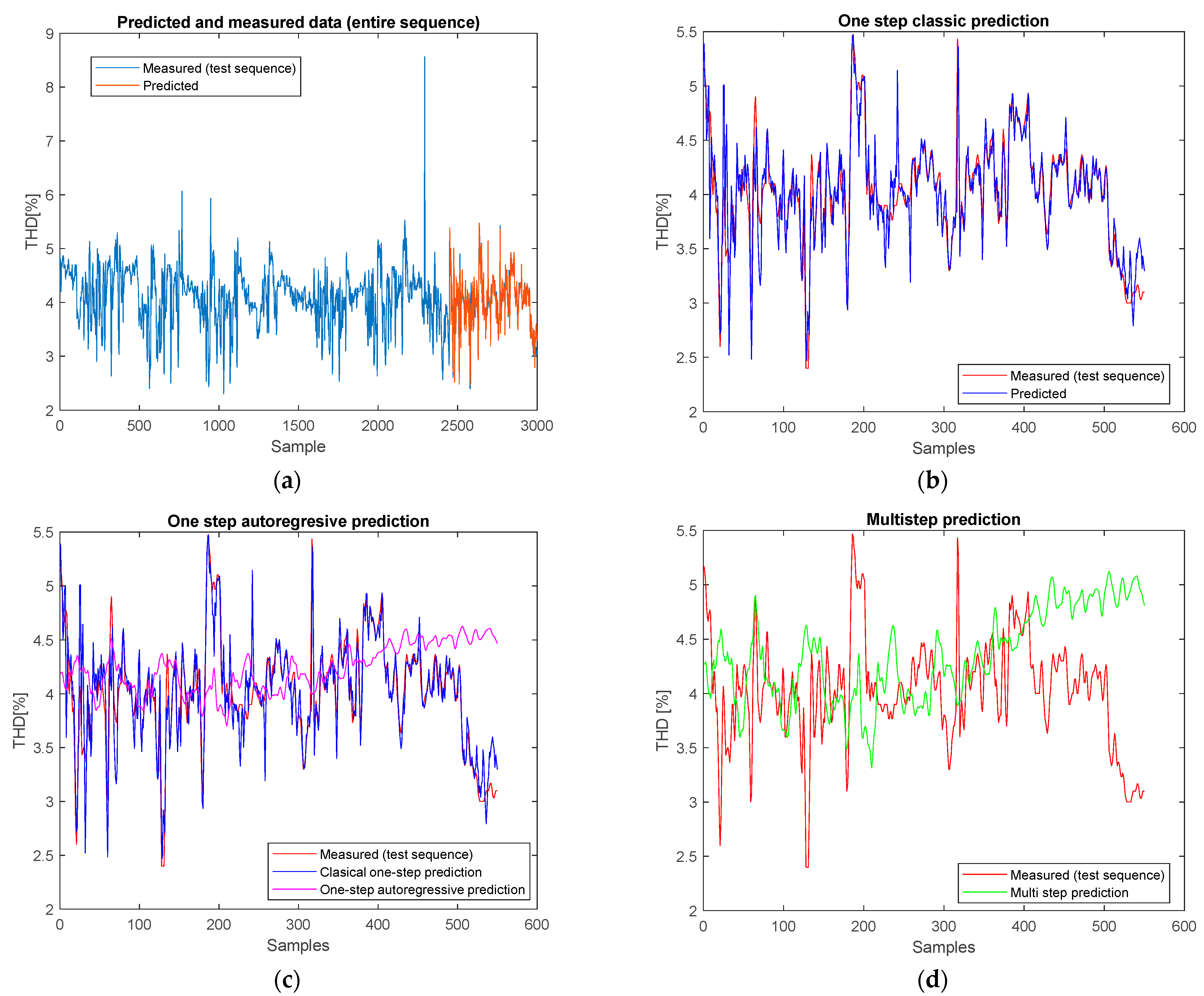
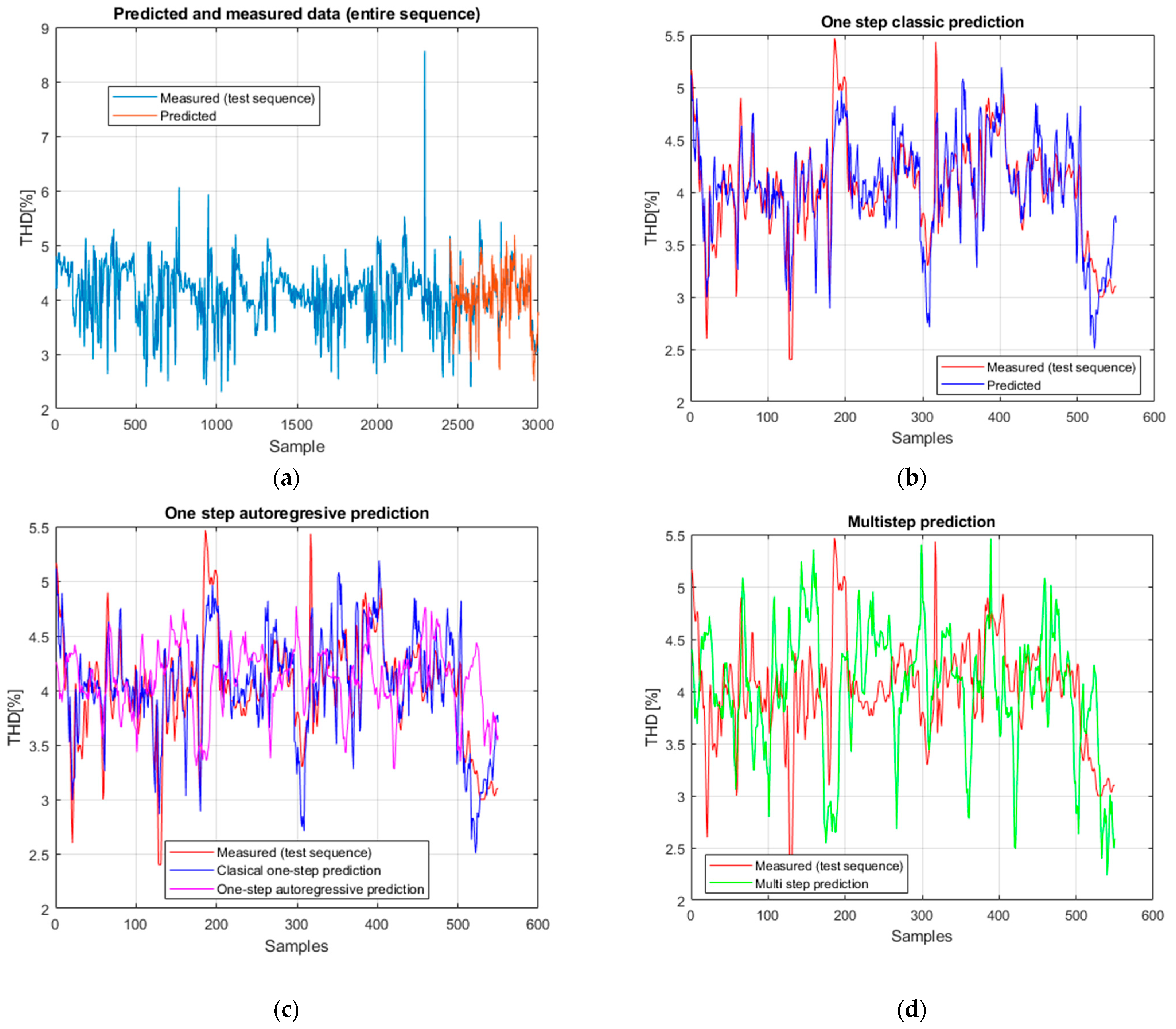
Figure 6a shows the measured data together with the predicted data on the training and testing sets, and from the representation it can be seen that the feedforward model manages to track the evolution of the THD values quite well. The quantitative evaluation of the performance for the classical prediction on the testing data (
Figure 6b) indicates very good values of the statistical indicators, with RMSE = 0.221150, MAE = 0.135831, sMAPE = 0.008772, and a correlation coefficient of ρ = 0.894739 (
p-value < 10
−189), which confirms a high correspondence between the measured and estimated data. In contrast, for the single-step autoregressive prediction (
Figure 6c), the performance degrades, obtaining RMSE = 0.570047, MAE = 0.435029, sMAPE = 0.027837, and a very weak correlation, ρ = −0.229568 (
p-value ≈ 5.196025 × 10
−8). In the case of multi-step prediction (
Figure 6d), the situation deteriorates further, with increased errors. The errors go up (RMSE = 0.718889, MAE = 0.569069, sMAPE = 0.569069), and the correlation stays low (ρ = −0.229148). This shows that errors rise up quickly and accuracy drops down over extended time periods. These results demonstrate that the feedforward architecture is suitable for classical point prediction; however, it shows significant deficiencies in autoregressive and multi-step techniques, where the absence of memory systems considerably reduces generalization capacity.
5.2. Results Using Recurent Neural Networks (RNN)
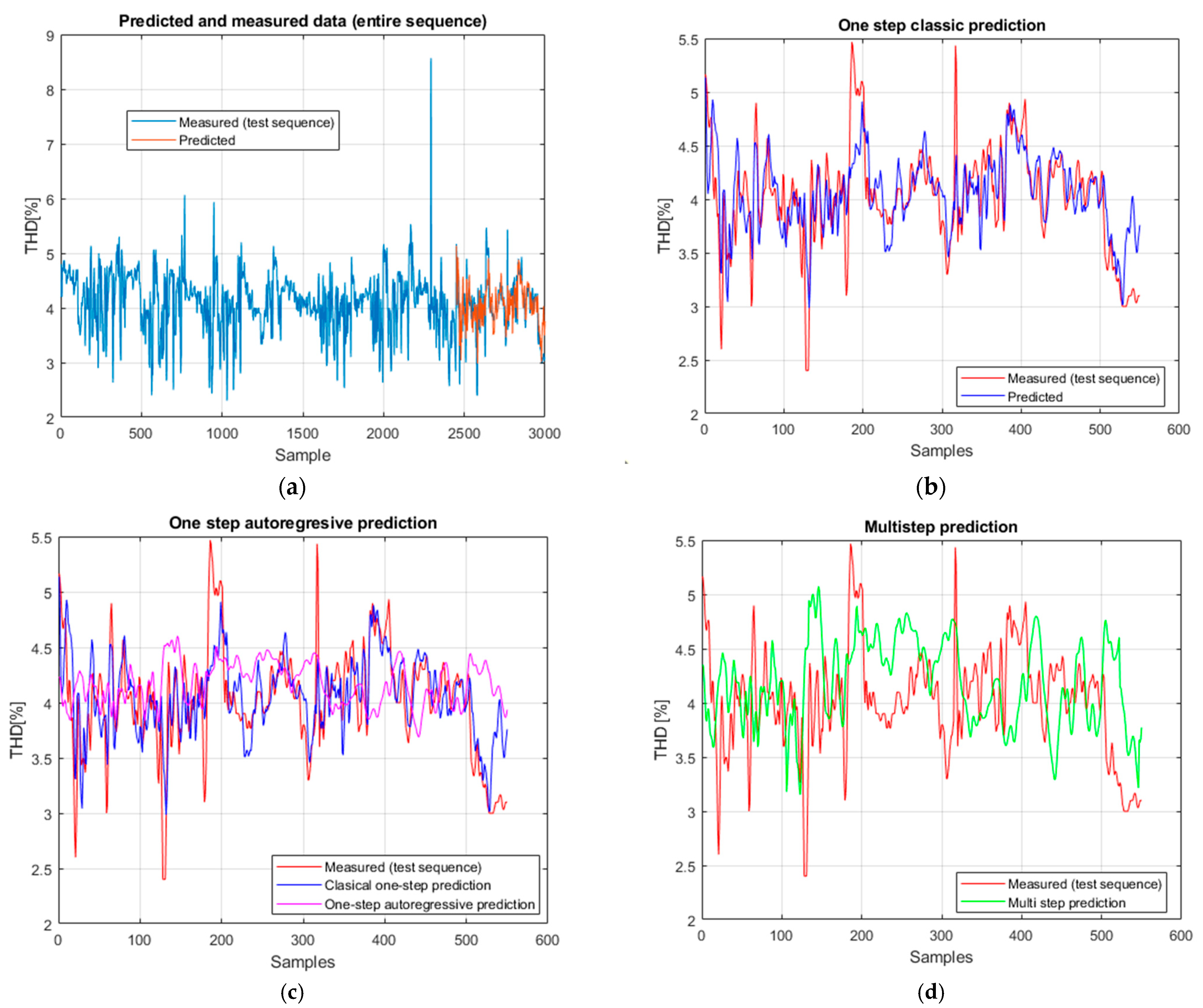
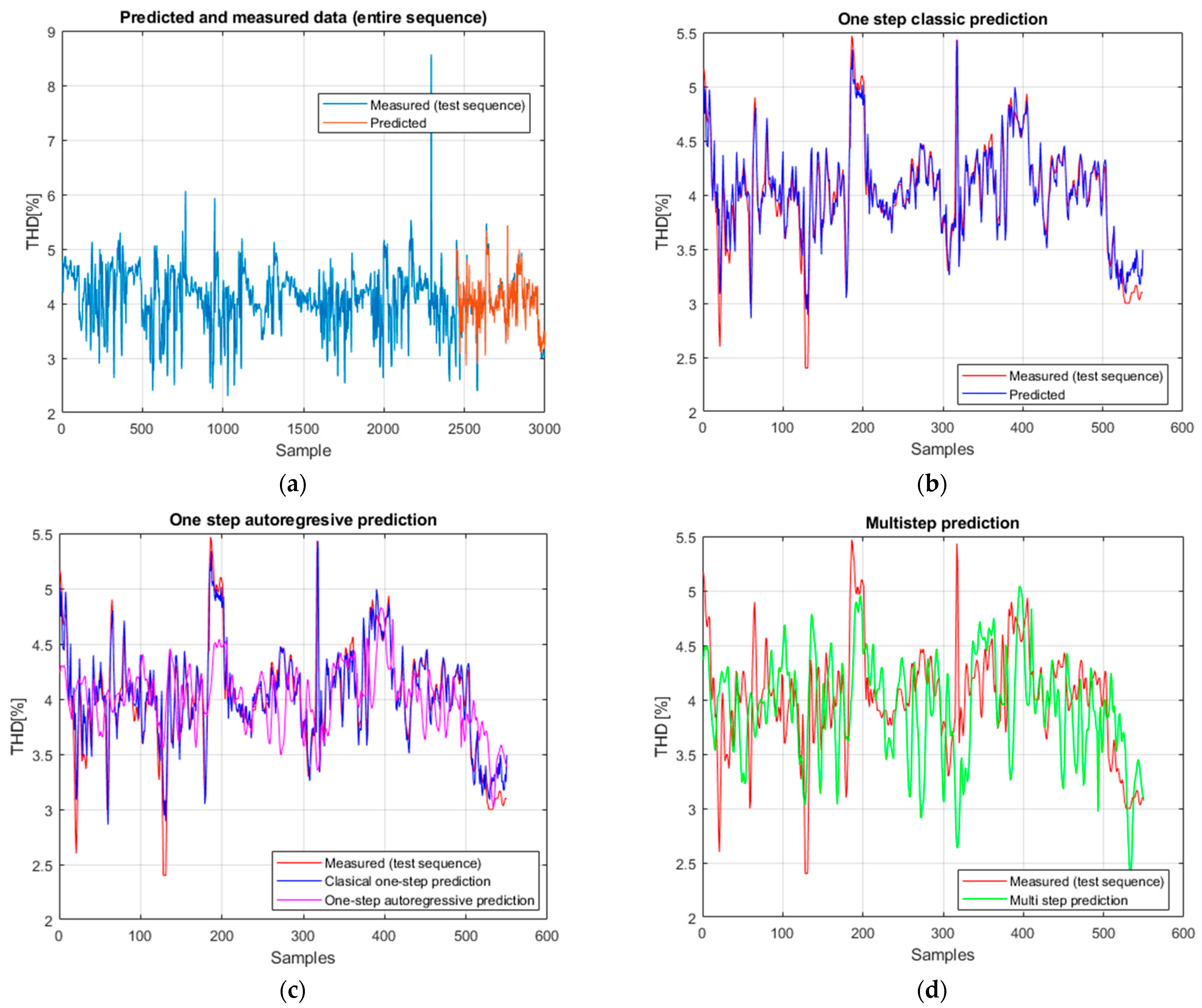
The results obtained for the RNN network (
Figure 7a–d) highlight a difference between the high performance in classical prediction and its limits in autoregressive and multi-step predictions.
In the case of the RNN network, the performance in classical prediction on the test set (
Figure 7b) is satisfactory, with the model being able to track the variations of the real values. The statistical indicators confirm this: RMSE = 0.2969, MAE = 0.2286, and sMAPE = 0.0146, with a high correlation coefficient ρ = 0.7927 and a coefficient of determination R
2 = 0.625. These results indicate that the model successfully identified the relationship between the input data and the desired outputs.
For the autoregressive prediction in a single step (
Figure 7c), the performance drops considerably. The values RMSE = 0.5969, MAE = 0.4544, and sMAPE = 0.0192 indicate an increase in errors, while the determination coefficient decreases to R
2 = 0.247, showing partial degradation due to the iterative propagation of prediction errors. Even though the Pearson correlation remains moderate (ρ = 0.584,
p < 0.001), the predictions begin to deviate from the real data dynamics. In the case of multi-step prediction (
Figure 7d), the results are similar: RMSE = 0.6166, MAE = 0.4813, sMAPE = 0.0253, and R
2 = −0.296, with a weak correlation (ρ = 0.227). Although the absolute errors remain moderate, the negative coefficient of determination highlights that the model fails to maintain a consistent explanation of the variability of the data over extended horizons.
In conclusion, RNN provides accurate prediction in the classical approach, but the accumulation of errors in the autoregressive and multi-step prediction significantly limits its long-term generalization capability.
5.3. Results with Gated Recurrent Unit (GRU)
The results for the GRU network (
Figure 8a–d) show a balanced performance, with excellent prediction in the classical regime and superior stability in the autoregressive and multi-step scenarios.
In the classical prediction on the test set (
Figure 8b), the GRU model reproduces the general evolution of the real values with moderate accuracy, obtaining RMSE = 0.3246, MAE = 0.2371, and sMAPE = 0.0150, with a correlation coefficient ρ = 0.746 and R
2 = 0.551. These values indicate a satisfactory but slightly weaker fit compared to the RNN.
For the one-step autoregressive prediction (
Figure 8c), the performance decreases noticeably, with RMSE = 0.5410, MAE = 0.4072, and sMAPE = 0.0271. The coefficient of determination becomes negative (R
2 = −0.328) and the correlation is weak (ρ = −0.104), showing that error accumulation significantly degrades prediction quality.
In the case of multi-step prediction (
Figure 8d), the results remain similar, with RMSE = 0.6469, MAE = 0.5103, sMAPE = 0.0319, R
2 = −0.690, and a very weak correlation (ρ = 0.056). Although the estimated series still follows the general shape of the signal, the low statistical indicators confirm that the GRU model fails to maintain consistency over extended horizons. Overall, the GRU provides only moderate accuracy in classical prediction and shows limited robustness in autoregressive and multi-step forecasting, performing slightly below the RNN in terms of long-term generalization.
5.4. Results with the Long Short-Term Memory (LSTM) Model
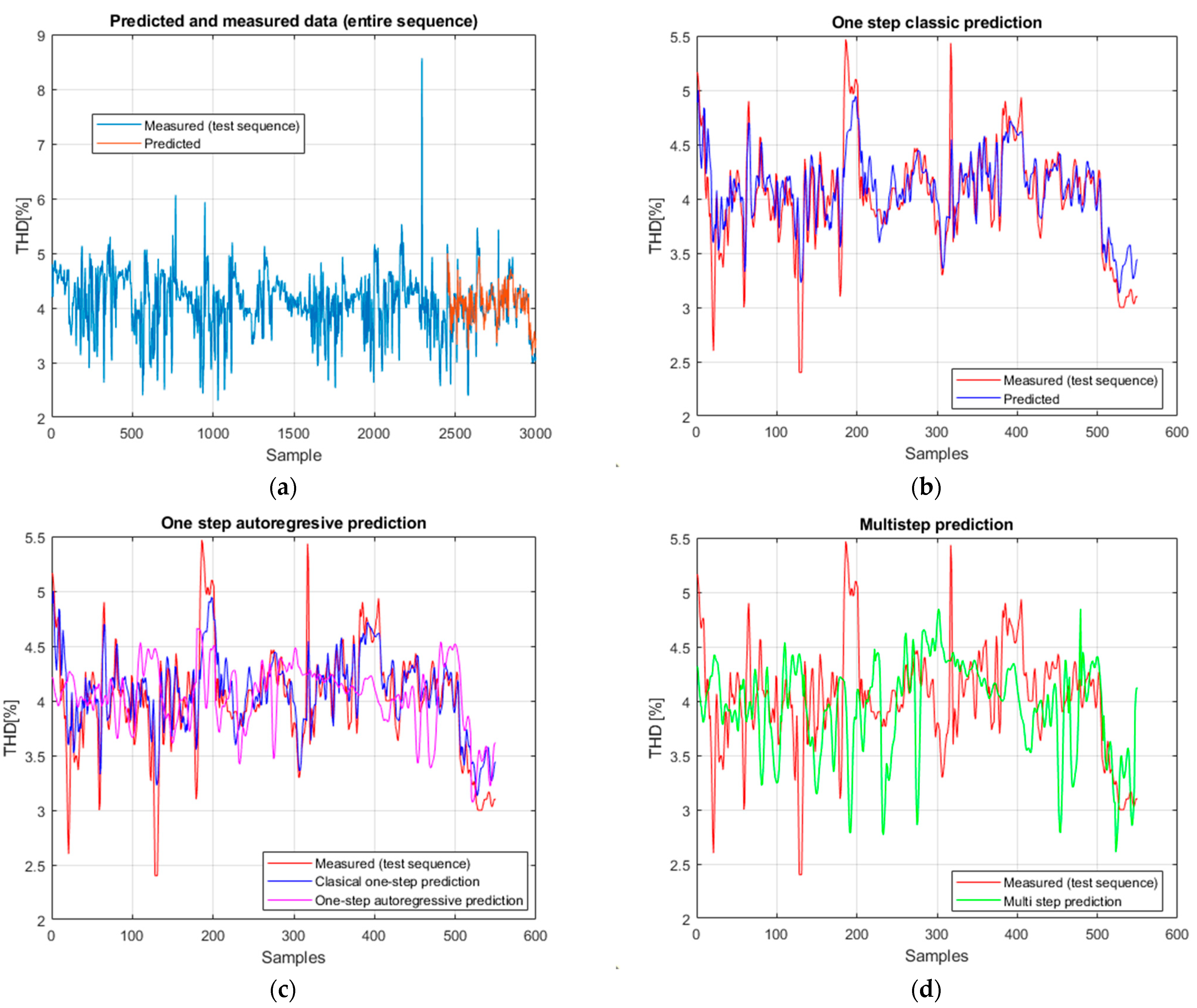
The LSTM network (
Figure 9a–d) shows robust behavior, with excellent accuracy in the classical regime and improved stability on extended horizons. The LSTM classical prediction on the test set (
Figure 9b) yields RMSE = 0.2571, MAE = 0.1870, sMAPE = 0.0119, ρ = 0.870, and R
2 = 0.718. The measured and predicted values correspond closely.
For the one-step autoregressive prediction (
Figure 9c), the performance decreases, with RMSE = 0.5809, MAE = 0.4479, and sMAPE = 0.0221, while the determination coefficient remains slightly positive (R
2 = 0.0257) and the correlation drops to ρ = 0.365 (
p < 10
−18). These results indicate that the accumulation of errors begins to affect the prediction quality, yet the model retains a weak but consistent correspondence with the real data.
In multi-step prediction (
Figure 9d), LSTM achieves RMSE = 0.6470, MAE = 0.5042, sMAPE = 0.0264, R
2 = −0.286, and a low correlation (ρ = 0.281,
p < 10
−11). While the negative R
2 values confirm the architecture’s limited ability to explain data variability over extended horizons, the predicted series still follows the main shape of the real data more coherently than in the one-step regime.
Even though the statistical values of the autoregressive and multi-step strategies show limitations, LSTM continues to perform well in classical prediction and demonstrates partial robustness against long-term error accumulation.
5.5. Results with Bidirectional LSTM (Bi-LSTM)
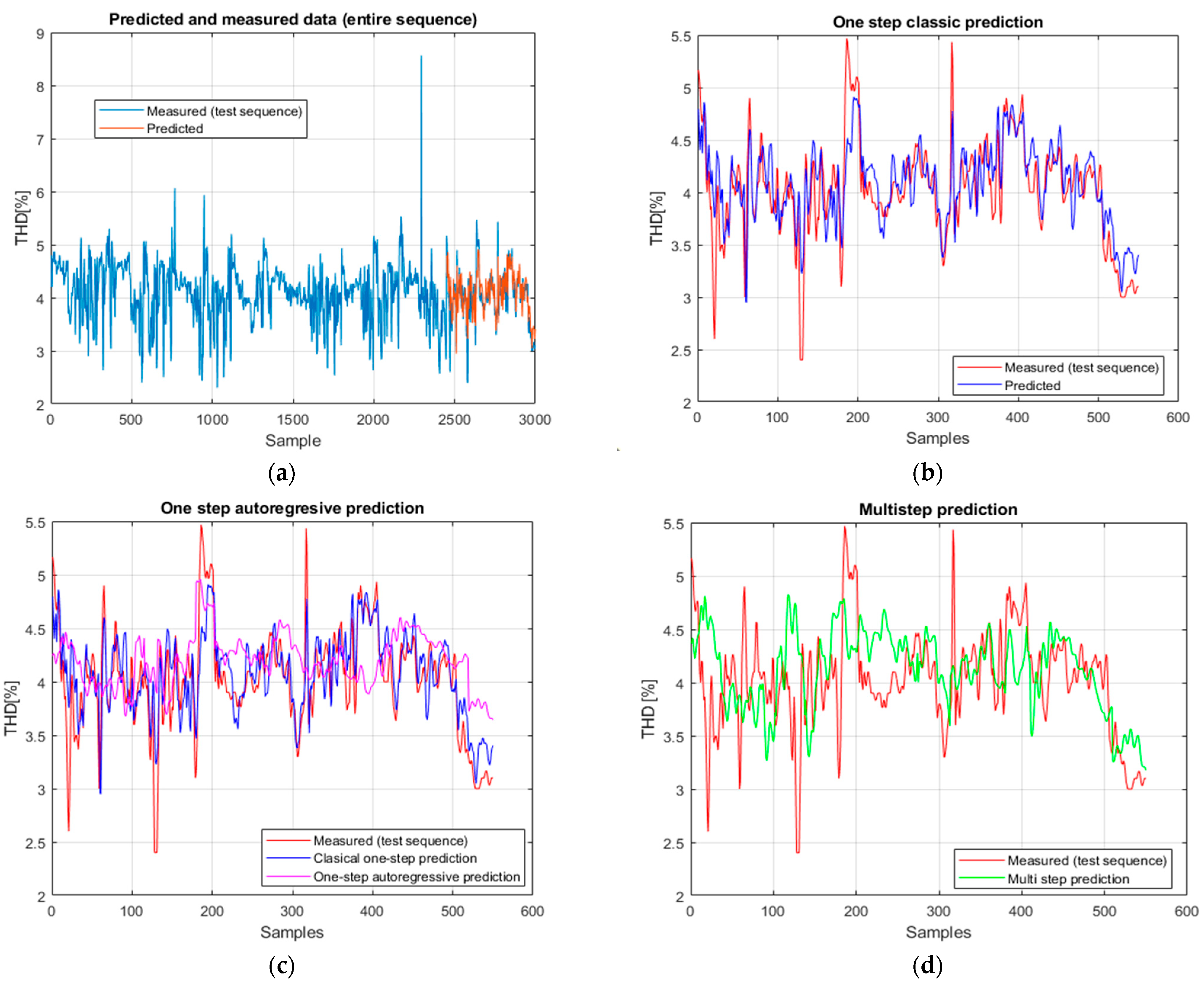
The results for the BiLSTM network (
Figure 10a–d) show a similar behavior to other recurrent architectures, with excellent performance in classical prediction and limitations in the autoregressive and multi-step regimes.
In classical prediction on the test set (
Figure 10b), BiLSTM obtains RMSE = 0.2805, MAE = 0.2132, sMAPE = 0.0135, correlation ρ = 0.832, and a coefficient of determination R
2 = 0.665. These results indicate a satisfactory fit between the measured and estimated data, demonstrating the model’s ability to capture bidirectional dependencies in the data used.
For the single-step autoregressive prediction (
Figure 10c), the performance decreases moderately, with RMSE = 0.5646, MAE = 0.4285, and sMAPE = 0.0233, while the determination coefficient remains close to zero (R
2 = 0.006) and the correlation drops to ρ = 0.353 (
p < 10
−17). These results suggest that the accumulation of errors slightly affects prediction quality, but the model retains a weak consistency with the real data.
In the case of multi-step prediction (
Figure 10d), the results are comparable: RMSE = 0.6146, MAE = 0.4792, sMAPE = 0.0215, with R
2 = 0.007 and a moderate correlation (ρ = 0.401,
p < 10
−22). Even though the statistical values highlight the model’s limited explanatory power, the visual representation shows that BiLSTM manages to follow the general trends of the real data, maintaining better stability over extended horizons.
Overall, BiLSTM offers good accuracy in the classical regime and relatively higher stability in multi-step predictions, but the accumulation of small errors still limits its long-term generalization capability.
5.6. Results with RNN with Self-Attention
The results for the self-attention RNN (
Figure 11a–d) show a strong integration between the recurrent mechanism and the ability of the attention layer to highlight important relationships within temporal sequences.
In the classical prediction regime (
Figure 11b), the model obtains RMSE = 0.2831, MAE = 0.2168, sMAPE = 0.0138, ρ = 0.834, and R
2 = 0.659. These results indicate that attention integration enhances the model’s ability to capture temporal dependencies, achieving high precision and a strong correlation between measured and predicted values.
The one-step autoregressive prediction (
Figure 11c) shows a moderate decrease in performance, with RMSE = 0.6164, MAE = 0.4726, sMAPE = 0.0190, ρ = 0.605, and R
2 = 0.317. These values demonstrate that, although iterative propagation increases errors, the model maintains a significant positive correlation with real data, confirming the stabilizing effect of the attention mechanism.
In the multi-step prediction (
Figure 11d), the results remain consistent, with RMSE = 0.6577, MAE = 0.5125, sMAPE = 0.0214, ρ = 0.515, and R
2 = 0.099. The positive R
2 values and moderate correlations indicate that the self-attention structure helps preserve temporal consistency over extended horizons, even though the predictive precision gradually decreases.
Overall, the self-attention RNN achieves high accuracy in classical point prediction and maintains improved robustness in the autoregressive and multi-step forecasts, demonstrating that the attention mechanism effectively enhances the recurrent architecture’s temporal learning capability.
5.7. Results Using Convolutional Neural Networks (CNN)
The results for the CNN network (
Figure 12a–d) show a satisfactory prediction capacity in the classical regime but also limitations in the autoregressive and multi-step predictions.
In the classical prediction on the test set (
Figure 12b), the CNN obtains RMSE = 0.204, MAE = 0.145, sMAPE = 0.0094, a correlation coefficient ρ = 0.913, and a coefficient of determination R
2 = 0.822. These results confirm good accuracy and a strong correlation between the measured and predicted values, demonstrating the efficiency of the convolutional architecture in extracting relevant local features.
For the one-step autoregressive prediction (
Figure 12c), the performance decreases, with RMSE = 0.581, MAE = 0.581, sMAPE = 0.0186, R
2 = 0.330, and a moderate correlation (ρ = 0.589). The results show that the model partially loses connection with the real series when previous predictions are reintroduced as inputs, which causes an increase in errors and a reduction in correlation strength.
In the case of multi-step prediction (
Figure 12d), the CNN obtains RMSE = 0.657, MAE = 0.513, sMAPE = 0.0222, ρ = 0.483, and R
2 = 0.043. Although the predicted series visually follow the general trend of the real data, the low R
2 values indicate that the model explains only a limited part of the data variability over extended horizons.
Overall, the CNN provides accurate prediction in the classical regime, but its performance deteriorates in the autoregressive and multi-step scenarios, where error accumulation and the absence of temporal memory significantly reduce long-term accuracy.
5.8. Results with Hybrid CNN-GRU-LSTM Architecture for Robust THD Forecasting
An advanced hybrid architecture combining convolutional layers (2D CNN) with recurrent GRU and LSTM layers was proposed to utilize both the ability to extract local features from sequential signals and the ability to capture long-term temporal relationships.
The input sequences were initially passed through a deep convolutional block, consisting of multiple 2D convolutional layers with progressive dilation factors (1, 2, 4, 8, and 16). This provides the network the ability to capture varying amplitude and frequency patterns in the input data. Each convolutional layer is followed by an ELU (Exponential Linear Unit) activation, which maintains the stability of the gradient propagation. A pooling layer is used to reduce the intermediate dimensionality.
After spatial feature extraction, the data is fed into a sequence of GRU and LSTM layers. The initial GRU provides efficient storage with a small number of parameters, while the subsequent LSTM layers are used to model complex temporal relationships. To prevent overfitting and improve generalization, dropout regularization layers are inserted between the recurrent layers.
Finally, the output is preceded by a fully connected layer, followed by a regression layer that produces the numerical prediction of the THD value.
The proposed CNN–GRU–LSTM hybrid architecture is shown in
Figure 13. It integrates convolutional and recurrent components to capture both local and long-term temporal dependencies in the THD signal. The network includes four convolutional layers (3 × 3 kernels, stride = 1, ELU activation, and batch normalization), followed by an average pooling layer and a flattening operation. The extracted features are processed by a GRU layer (100 units) and an LSTM layer (100 units) in sequence, with dropout regularization (rate = 0.2) between layers. A fully connected regression output layer completes the model.
This architecture was optimized empirically through iterative tuning of convolutional filters and recurrent units, resulting in a balanced configuration that ensured both prediction accuracy and computational efficiency.
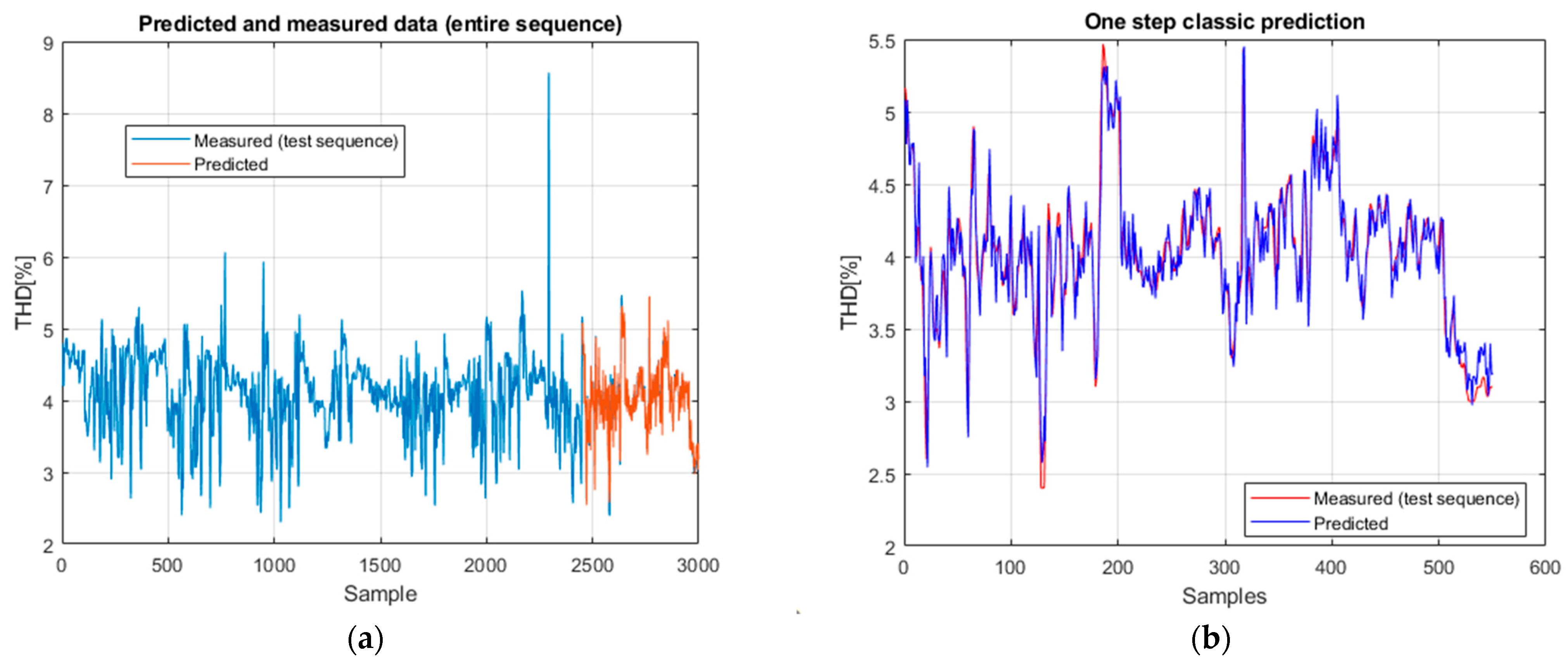
The hybrid model achieves very good performance in classical prediction: RMSE = 0.134, MAE = 0.097, sMAPE = 0.0063, with a very high correlation (ρ = 0.961) and a coefficient of determination of R2 = 0.923. These values confirm that the hybrid architecture manages to capture both local features (through the convolutional part) and long-term temporal dependencies (through GRU and LSTM). Practically, the predictions overlap almost perfectly with the measured data.
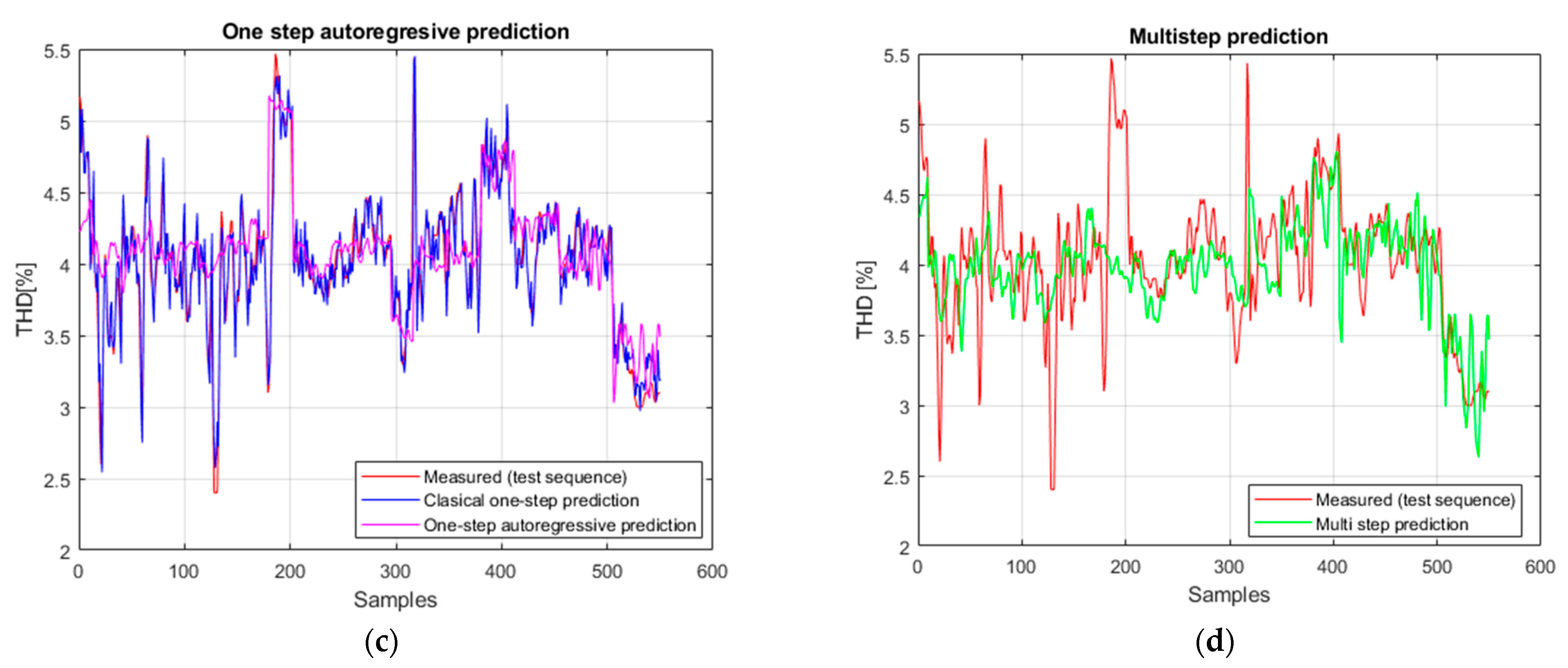
In autoregressive prediction, as observed in the other architectures, the performance decreases due to the accumulation of errors. However, in this case, the degradation is moderate: RMSE = 0.611, MAE = 0.458, sMAPE = 0.0156, with a positive R
2 = 0.437 and correlation ρ = 0.683. These results show that the hybrid model retains a strong capacity to preserve the signal trend, effectively limiting error propagation compared to the other networks. The results are presented in
Figure 14.
For multi-step prediction, the results remain stable and robust: RMSE = 0.620, MAE = 0.472, sMAPE = 0.0171, with R2 = 0.430 and a significant correlation (ρ = 0.669). This demonstrates that, unlike other architectures where multi-step predictions deteriorated rapidly, the hybrid model maintains consistency with the real signal and successfully reproduces its dynamics over extended horizons.
The measurements were performed in a single steel mill; however, the data acquisition included multiple operating cycles, over several days, that included transient events, steady-state periods, and switching of the reactive power compensation facility. These variations produced a diverse set of signal patterns, including frequent transients, harmonic fluctuations, and changes in reactive power flow, which allowed the models to learn from a rich and heterogeneous data set. Therefore, the sampling duration and the diversity of operating regimes were sufficient to characterize the dynamic behavior of the system under real industrial conditions. In addition, to improve generalization, the data set was divided into independent training, validation, and testing subsets to ensure that unseen data segments were used for performance evaluation. The predictive models—especially the CNN-GRU-LSTM hybrid—demonstrated consistent accuracy and stable correlation metrics (R2 and ρ) in these unused training data sequences, confirming their ability to generalize to new operational scenarios, rather than simply memorizing specific models.
6. Discussion
The comparative results of all architectures across the three prediction strategies are summarized in
Table 2, which reports the values of RMSE, MAE, sMAPE, the coefficient of determination (R
2), the Pearson correlation coefficient (ρ), and the associated
p-values. These results allow for a detailed discussion on the relative performance, robustness, and limitations of each model.
The comparative analysis of the tested neural network architectures highlights important differences in their behavior for the three prediction methods (classical, autoregressive one-step, and multi-step).
In the case of classical prediction on the test data, the results confirm the theoretical expectation that convolutional and hybrid architectures provide the highest accuracy. However, several recurrent models also performed well. The feedforward network achieved strong results (R2 ≈ 0.79, ρ ≈ 0.89), showing that even a simple architecture can effectively capture short-term dependencies. Among recurrent models, the LSTM also showed robust performance (R2 ≈ 0.72, ρ ≈ 0.87), confirming its ability to model nonlinear temporal dynamics. The BiLSTM and RNN with self-attention offered slightly lower but still consistent accuracy (R2 ≈ 0.65–0.66, ρ ≈ 0.83–0.84), while the standard RNN and GRU achieved moderate performance (R2 ≈ 0.55–0.62, ρ ≈ 0.74–0.79).
The Enhanced Hybrid CNN–GRU–LSTM achieved the best overall performance, with very low error rates (RMSE = 0.134, MAE = 0.097, sMAPE = 0.0063), a very strong correlation with the real data (ρ = 0.961, p < 0.001), and the highest coefficient of determination (R2 = 0.923). These results show that the hybrid model effectively captures both local features (via convolutional layers) and long-term temporal dependencies (through GRU and LSTM units), making it ideally suited for the analyzed THD data.
The CNN model also achieved very good results (R
2 = 0.822, ρ = 0.913), confirming the ability of convolutional architectures to extract meaningful local patterns from sequential signals. Related studies have reported similar conclusions, showing that CNN–LSTM hybrids improve forecasting accuracy in solar irradiance prediction [
32] and electricity consumption estimation [
33].
When using autoregressive one-step prediction, all models’ performance dropped significantly. This is in line with the theory that recursive prediction propagates and amplifies errors. For every model, the R
2 values became significantly smaller, sometimes negatives (from −0.588132 to 0.437422), which meant that the models explained less variance than a simple predictor that only returned the mean of the data. Such negative coefficients of determination are consistent with prior observations in the literature, which demonstrate that recursive forecasting methods inherently accumulate uncertainty and gradually lose coherence with the real data [
34]. In the context of this study, the GRU model, despite its gating mechanism, experienced a notable degradation of predictive accuracy under recursive conditions, confirming observations from earlier studies on the difficulty of maintaining gradient stability in gated networks during iterative forecasting [
34]. By contrast, recurrent models such as RNN, LSTM, BiLSTM, and RNN with self-attention maintained positive R
2 values (0.02–0.32) and moderate correlations (ρ ≈ 0.35–0.68), indicating that they retained partial coherence with the measured data. The Enhanced Hybrid CNN–GRU–LSTM model achieved the best autoregressive performance, maintaining a high correlation (ρ = 0.683) and a positive R
2 = 0.437, demonstrating that the hybridization of convolutional and recurrent layers significantly improves recursive stability. These results align with research on error mitigation in recurrent forecasting, which shows that gating mechanisms can limit the accumulation of errors over extended horizons [
35], as well as studies that emphasize the benefits of improved gating structures in recurrent neural networks [
36]. In contrast, the Feedforward architecture exhibited the weakest autoregressive performance, with a strongly negative R
2 and high absolute errors, confirming that models without temporal memory are most affected by recursive feedback and error accumulation.
Although the overall accuracy did not increase, the degradation of performance was more gradual, indicating that the multi-step approach provided improved stability across extended horizons. This behavior reflects the fact that direct multi-step forecasting, unlike recursive strategies, produces predictions directly for the future interval rather than reusing previous outputs as new inputs. As a result, it limits the exponential accumulation of propagated errors, even when the global accuracy remains similar to or slightly below that of the one-step regime. These results are consistent with other studies reporting that direct multi step methods mitigate the instability typical of iterative approaches [
37].
In the current research, most architectures achieved near-zero or slightly negative R2 values (−0.29 to 0.10), with moderate correlations (ρ ≈ 0.40–0.67), indicating partial robustness in tracking long-term dynamics. Notably, several models obtained positive R2 values in this regime—specifically, the BiLSTM (R2 ≈ 0.007), CNN (R2 ≈ 0.043), RNN with self-attention (R2 ≈ 0.099), and the Enhanced Hybrid CNN–GRU–LSTM (R2 ≈ 0.430). These results demonstrate that the inclusion of bidirectional or attention mechanisms, and especially the hybrid combination of convolutional and recurrent layers, enhances the network’s ability to preserve temporal consistency over longer horizons.
By contrast, Feedforward, GRU, LSTM, and RNN exhibited negative R2 values (ranging from −0.29 to −0.69), yet maintained relatively low errors (RMSE ≈ 0.61–0.66), suggesting that even when explanatory power decreases, the models still retain a reasonable capability to approximate the overall signal trend.
These outcomes align with observations in the time-series forecasting literature, particularly within attention-based and hybrid architectures. For example, transformer architectures are often preferred in multi-step forecasting tasks due to their ability to reduce long-term error accumulation and preserve sequential coherence [
38]. Furthermore, hybrid deep learning methods have demonstrated superior accuracy in long-horizon prediction problems, such as coal price forecasting and other complex dynamic domains [
39].
Overall, several conclusions can be drawn. In classical prediction, convolutional and hybrid architectures remain superior, with the Enhanced Hybrid CNN–GRU–LSTM achieving the highest accuracy. In the autoregressive regime, all models exhibit performance degradation due to recursive error propagation, though networks with memory—such as GRU, LSTM, BiLSTM, and the hybrid—retain better stability than the Feedforward and CNN models. In multi-step forecasting, direct prediction over extended horizons limits, but does not eliminate, error accumulation; several architectures, including BiLSTM, CNN, the attention-based RNN, and the hybrid model, maintain positive R2 values and moderate correlations. Finally, while correlations remain high in the classical regime (>0.90), they decrease in autoregressive mode and partially recover in multi-step forecasting, reflecting the stabilizing effect of direct multi-horizon prediction on temporal coherence.
Negative R
2 values were obtained for some architectures in the autoregressive mode—mainly Feedforward and GRU—indicating weaker performance due to recursive error accumulation. This behavior is typical and consistent with reports in the recent time-series literature [
40,
41]. In contrast, models with memory and gating mechanisms, such as LSTM, BiLSTM, and the hybrid CNN–GRU–LSTM, maintained positive R
2 values and moderate correlations (ρ ≈ 0.35–0.68), showing better resistance to error propagation.
In conclusion, the comparative evaluation shows that hybrid architectures, particularly the Enhanced CNN-GRU-LSTM, are the most effective choice for THD prediction, offering both useful short-term accuracy and superior robustness in long-term forecasting scenarios.
In addition to the prediction performance criteria, the computational efficiency of the tested models was evaluated to determine whether they were suitable for real-time applications. For the purpose of accurate comparison, all neural network architectures were trained on the same datasets with the same hyperparameters (600 epochs, MiniBatchSize = 128, initial learning rate = 0.008). Although more complex architectures required longer training times, the CNN-GRU-LSTM hybrid network is computationally acceptable, with training taking only a few tens of minutes on a mid-range GPU. The inference speed of the CNN–GRU–LSTM model was tested on a computer with an Intel i7 processor and an NVIDIA RTX 3060 GPU. Once trained, the model performs THD prediction with high computational efficiency, requiring less than 0.5 s on the CPU and less than 0.1 s on the GPU for a 10-step forecast window. These results demonstrate that the proposed hybrid architecture is suitable for near-real-time power quality prediction. Consequently, the model can be integrated into real-time monitoring and predictive control frameworks without additional hardware acceleration.
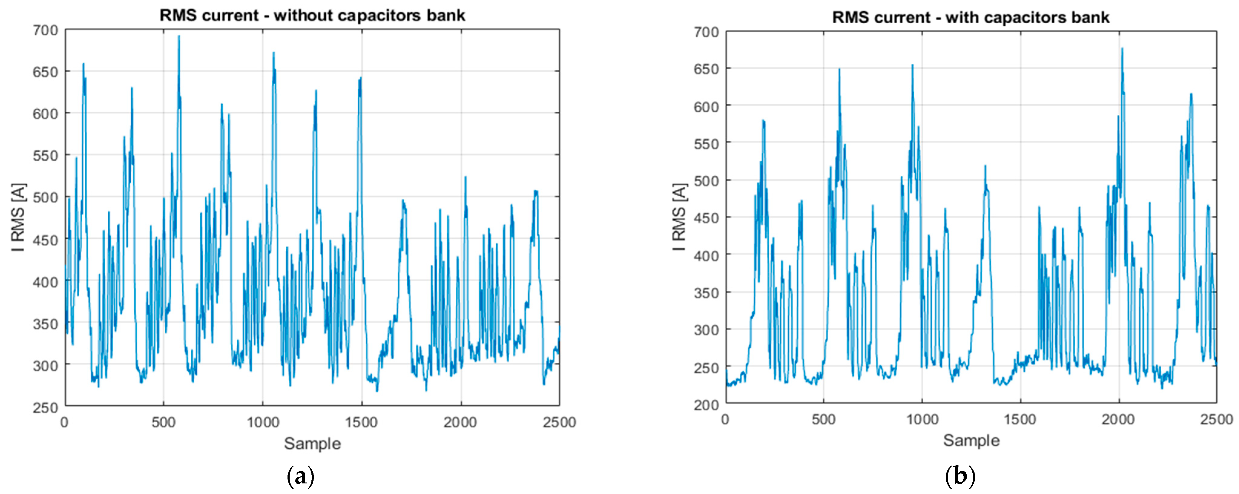
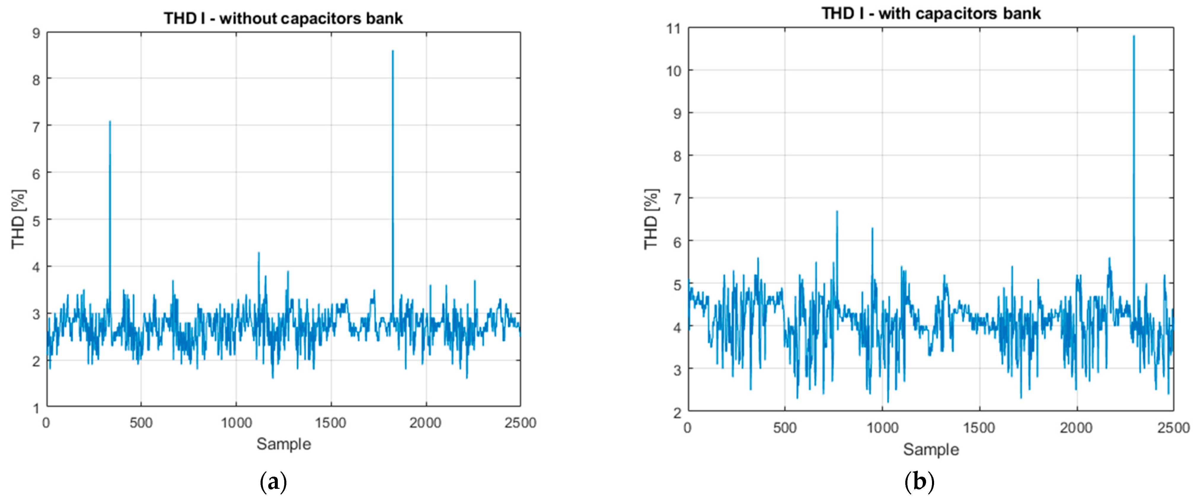
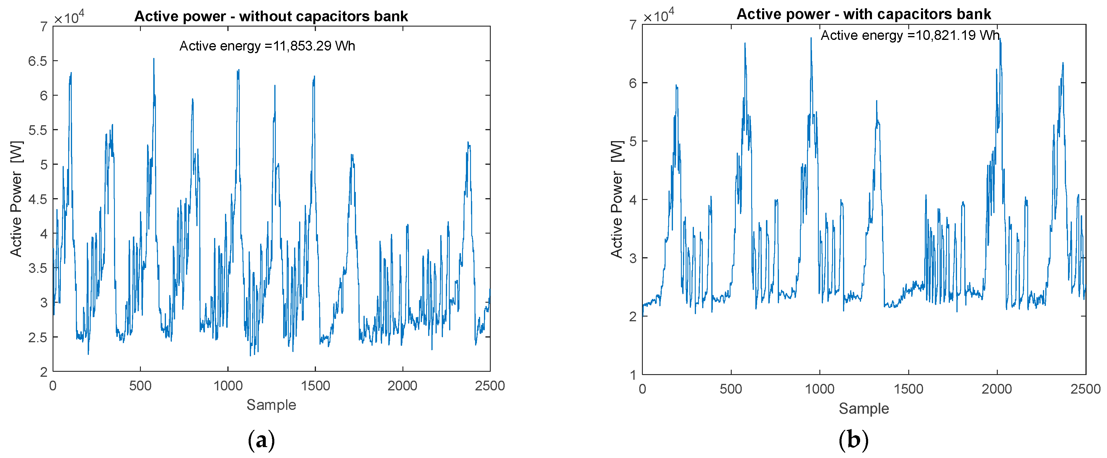
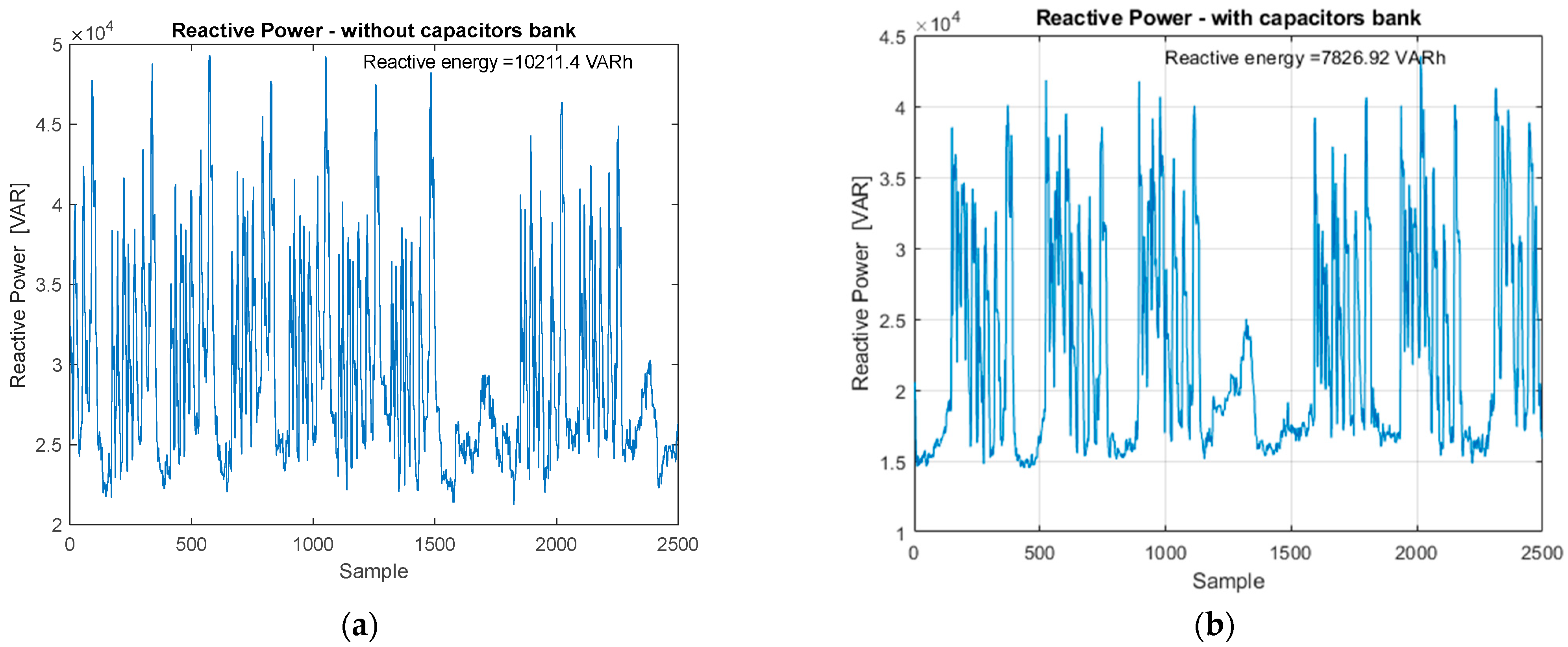
The experimental data used for the model development included numerous sequences with sudden and repetitive variations of current, THD, and active/reactive power, which show frequent transient conditions. These data characterize dynamic regimes—with current peaks exceeding 650 A and THD increases of up to 7–8.5%—and are the real input data that were used by the neural network architectures, and thus they were able to learn from real operating fluctuations. The proposed CNN-GRU-LSTM hybrid architecture efficiently learned both short-term transient characteristics and long-term temporal dependencies, which makes it suitable for modeling the nonlinear behavior of THD under such variable load conditions. Although the model does not explicitly classify the operating regimes, it implicitly learns their patterns from the training data. Through experiments performed in both compensated and uncompensated regimes, the network correctly identified the correlations between power variations and distortion peaks. This confirms the model’s ability to adapt to real industrial operating conditions and to provide a good and stable forecast of harmonic distortion during frequent load transitions.
All models were validated using standard indicators, including RMSE, MAE, sMAPE, R2, and Pearson correlation coefficient (ρ). These metrics provide a comprehensive evaluation of accuracy, error magnitude, and temporal continuity. The CNN-GRU-LSTM hybrid model outperformed all other studied architectures in terms of predictive accuracy and robustness, with R2 = 0.923 and ρ = 0.961 in classical prediction and a positive R2 (0.285) in multi-step prediction. These results confirm the model’s capacity for working consistently and accurately in the face of unpredictability. Furthermore, the prediction of THD progress allows the early detection of power quality issues and the implementation of proactive compensation or filtering actions, resulting in a more resilient power supply system for rolling mills.
7. Conclusions
This paper presented a comprehensive analysis of total harmonic distortion (THD) prediction using various neural network architectures, including feedforward networks, recurrent architectures (RNN, GRU, LSTM, BiLSTM), convolutional models (CNN), attention-based variants, and hybrid methods that combine CNN and recurrent units. The study systematically evaluated these models’ performance using three prediction methods: classical prediction on test data, autoregressive one-step prediction, and multi-step prediction.
The results show that architectural choices have an important effect on predicted accuracy and robustness. In classical prediction, convolutional and hybrid architectures performed better, with the Enhanced Hybrid CNN-GRU-LSTM appearing as the most effective model, with the lowest error values and the highest correlation with real data. In autoregressive one-step prediction, every architecture degraded significantly due to recursive error propagation, although recurrent models with gating mechanisms (GRU, LSTM, BiLSTM) and hybrid architectures demonstrated relative stability. The Enhanced Hybrid CNN-GRU-LSTM was the only architecture that achieved a positive R2, showing its resilience in long-term forecasting.
Overall, the comparative study emphasizes the advantages of combining convolutional and recurrent structures in a single hybrid framework. Such architectures offer both superior short-term accuracy and increased durability in long-term prediction tasks, making them ideal for use in power quality monitoring and industrial systems.
The comparative evaluation and optimization procedures applied in this study are consistent with current best practices in hybrid intelligent modeling and predictive system design [
38].
Future research will focus on increasing the adaptability of recursive prediction modes, integrating advanced attention mechanisms, and testing the suggested models on larger and more varied datasets to demonstrate their generalizability.
The proposed CNN–GRU–LSTM model can be integrated as a predictive module within supervisory control or energy management systems for industrial facilities (such as SCADA platforms). In this way, measures could be taken, and proactive compensation and control actions could be performed, such as adaptive regulation of reactive power compensators and automatic switching of harmonic filters. By predicting the trends of future THD values in real time, the model can help in decisions aimed at maintaining voltage stability and improving power quality and thus can contribute to reducing energy consumption and extending the lifetime of equipment.
Future work will focus on proposing a closed-loop predictive control framework using the developed model.

