Article

High-Order Special Two-Derivative Runge–Kutta Pairs

by
Ibraheem Alolyan
1,
Theodore E. Simos
2,3,* and
Charalampos Tsitouras
4
1
Department of Mathematics, College of Science, King Saud University, P.O. Box 2455, Riyadh 11451, Saudi Arabia
2
Center for Applied Mathematics and Bioinformatics, Gulf University for Science and Technology, West Mishref, Hawally 32093, Kuwait
3
Section of Mathematics, Department of Civil Engineering, Democritus University of Thrace, 67100 Xanthi, Greece
4
General Department, National & Kapodistrian University of Athens, Euripus Campus, 34400 Psachna, Greece
*
Author to whom correspondence should be addressed.
Mathematics 2025, 13(22), 3676; https://doi.org/10.3390/math13223676
Submission received: 28 September 2025 / Revised: 10 November 2025 / Accepted: 11 November 2025 / Published: 17 November 2025

Abstract

This paper presents the development and analysis of novel explicit special two-derivative Runge–Kutta (STDRK) pairs for the numerical integration of ordinary differential equations (ODEs), with a focus on achieving seventh-order accuracy and embedded fifth-order error estimation. The proposed schemes utilize both the first and second derivatives of the solution, leveraging the identity y = f ( y ) f ( y ) , to attain high-order accuracy while minimizing the number of evaluations of the primary function f. A notable feature of the constructed methods is that they require only a single evaluation of f per step, along with five evaluations of g = f f , resulting in a significant reduction in computational cost compared to classical Runge–Kutta methods. The necessary order conditions are derived via an algebraic framework based on compositions with parts not exceeding 2. A supporting Mathematica package facilitates the construction of methods of arbitrary order. A new STDRK pair of orders seven and five is derived. Numerical experiments on standard benchmark problems, including the Prothero–Robinson, Kaps, and Kepler systems, highlight the efficiency and competitive performance of the proposed schemes relative to established Runge–Kutta pairs.
MSC:
65L05; 65L06; 05C05; 68W30

1. Introduction

The task of numerically solving systems of ordinary differential equations
d y d t = f ( y ( t ) ) , y ( t 0 ) = y 0 , y ( t ) R μ , f : R μ R μ
has been a central topic in computational mathematics for over a hundred years. The design and analysis of general-purpose one-step methods, in particular, Runge–Kutta (RK) formulas, is by now a mature field, with detailed order theory, stability analysis, and extensive numerical experimentation [1,2,3,4]. Classical RK methods rely solely on evaluations of the right-hand side of function f, and their success stems from their simplicity, reliability, and wide applicability. Nevertheless, as the complexity of applications continues to increase, classical RK methods often struggle to meet the modern demands of efficiency, accuracy, and structure preservation.
A crucial observation is that, for autonomous systems, additional information is available through the second derivative of the solution:
y ( t ) = g ( y ( t ) ) = f ( y ( t ) ) f ( y ( t ) ) ,
where f ( y ) denotes the Jacobian of f at y. When f and f ( y ) are available, the evaluation of g ( y ) is straightforward. This opens the way to the development of methods that exploit both first- and second-derivative information. Special Two-derivative Runge–Kutta (STDRK) methods form a natural extension of the RK framework and have been studied from both the theoretical and practical perspectives [5]. By augmenting the stage structure with evaluations of g, one can construct schemes that reach higher algebraic order with fewer stages, thus reducing computational cost.
It should be noted that the restriction to autonomous systems does not diminish generality: a non-autonomous system y ( t ) = f ( t , y ) can always be rewritten in autonomous form by introducing an additional variable t satisfying t = 1 . This reformulation ensures that the framework of STDRK methods is applicable to the general case.
The algebraic foundation of STDRK methods is based on Taylor expansions involving both f and g, which result in fewer order conditions compared to the standard RK case. The additional degrees of freedom arising from the presence of g allow explicit methods with fewer stages and implicit methods with improved stability. For oscillatory or stiff problems, where classical explicit RK methods often require prohibitively small step sizes, such enriched methods can offer significant efficiency gains. In large-scale problems with y ( t ) R μ of high dimension, where each function evaluation may be costly, reducing the number of function evaluations per step is particularly important.
In this paper, we focus on a special subclass: explicit STDRK methods of minimal cost. The distinctive feature of these schemes is that they require only a single evaluation of the vector f per step. The higher order is then achieved by incorporating several evaluations of g = f f at suitably defined internal stages. Explicit s-stage formulas of this type advance the solution from ( t n , y n ) to ( t n + 1 = t n + h n , y n + 1 ) and can be written as
Y = e y n + h n c f ( y n ) + h n 2 ( A I μ ) G ( Y ) ,
y n + 1 = y n + h n f ( y n ) + h n 2 ( b I μ ) G ( Y ) ,
where I μ R μ × μ the identity matrix, e = ( 1 , , 1 ) T R s , c R s denotes the vector of stage nodes, A R s × s and weight row-vector b R 1 × s are coefficient arrays associated with the g-stages, and  G ( Y ) is the vector collecting evaluations of g at the internal stages Y. The use of Kronecker product notation emphasizes that these schemes are formulated to address general vector-valued problems. The explicit character of the method is maintained by considering the matrix A to be strictly lower triangular, thereby ensuring that the number of function evaluations per integration step is kept to a minimum.
As usual, we accompany the above formula with a costless lower-order evaluation
y ^ n + 1 = y n + h n f ( y n ) + h n 2 ( b ^ I n ) G ( Y ) ,
that ensures a local error estimation of the error
δ = y n + 1 y ^ n + 1
which is useful for adjusting h n for the next step.
At each step, the local error δ is compared with a predetermined tolerance τ . Whenever δ τ , we proceed with accepting the approximation y n + 1 and choose a new step for advancing the solution according to the formula
h n + 1 = 0.8 · h n · τ 1 p · δ 1 q + 1 ,
with 0.8 a safety factor, p the algebraic order of the higher-order method (i.e., with weights b) and q the order of the lower-order method, i.e., with weights b ^ . In the opposite case, we reject the step and we begin again with the procedure, but in the above formula, h n + 1 serves as a smaller new length for h n . See [6] for details in step size control algorithms and also [7,8].
This class of methods has several appealing advantages. First, for a given number of stages, higher algebraic order can be achieved compared to classical RK schemes. Second, by involving only one evaluation of f, the most costly part of the step is minimized, making these schemes particularly attractive in high-dimensional problems. Third, the improved phase accuracy and stability that comes with the use of g renders them efficient tools for oscillatory problems. This is especially relevant in mechanics, molecular dynamics, and other areas where solutions are highly oscillatory and long-time integration is required. As shown in previous work on two-derivative methods [9], the availability of higher-derivative information can dramatically reduce phase errors and improve long-term energy behavior.
Derivative-based and high-order numerical schemes have found applications in control-oriented problems involving PDE–ODE coupling, where stability and computational efficiency are both crucial. For instance, Xu and Li developed a semi global stabilization framework for parabolic PDE–ODE systems under input saturation, illustrating the importance of accurate time-integration schemes for ensuring closed-loop stability. They link PDE–ODE system stabilization with accurate numerical integration and control, aligning conceptually with the motivation for efficient, high-order methods like STDRK for complex dynamical systems [10].
The development of energy-stable and structure-preserving schemes remains a major concern in numerical analysis, particularly for nonlinear diffusion-type problems, such as the Allen–Cahn equation [11]. Although our present work focuses on ODE systems, the proposed STDRK framework could be extended toward PDE discretizations, where stability and derivative information play key roles. This provides a bridge between the presented ODE-based STDRK scheme and PDE applications where similar numerical stability concepts apply.
Similar to recent advances in unconditionally stable time-domain methods, such as the piecewise Chebyshev finite-difference schemes [12], the present STDRK method seeks to achieve both stability and computational efficiency by exploiting derivative information without increasing function evaluations.
The aim of the present paper is to advance the study of such special explicit STDRK methods. We develop their order conditions, produce a specific pair of orders 7 ( 5 ) and demonstrate their effectiveness through numerical experiments. Through a meticulous construction of schemes in this form, we derive explicit methods that achieve a balance of low computational cost, high order accuracy, and superior performance on oscillatory as well as other benchmark problems. These methods provide a compelling alternative to traditional explicit RK formulas, bridging the gap between classical one-derivative integrators and structure-adapted schemes.

2. Order Conditions Derivation

Building upon the comprehensive analysis in [5] for a broader class of methods, we introduce a more convenient framework for deriving the order conditions pertinent to the methods considered in this work.
Firstly, the problem is based on compositions of integer r 3 with no part greater than 2. Let this number be denoted by F ( r ) . In other words, we seek the number of ordered sums of positive integers (compositions) of r 3 , where each part is either 1 or 2.
A composition of a number is a way of writing it as a sum of positive integers where the order of the summands matters. We are interested in compositions of r 1 where each part is either 1 or 2. Let us compute the values of F ( r ) for small r in Table 1.
We observe that:
F ( r ) = F ( r 1 ) + F ( r 2 )
This is the recurrence relation for the Fibonacci sequence. That is, the number of compositions of r 1 with parts no greater than 2 equals the ( r 1 ) -th Fibonacci number.
Let us concentrate on the derivation of seventh-order equations. We observe that 4 = 7 3 can be summed with five different ways, assuming no number greater than 2 is involved. That is,
2 + 2 , 2 + 1 + 1 , 1 + 2 + 1 , 1 + 1 + 2 , 1 + 1 + 1 = 1 .
This is associated with letters
( A , A ) , ( A , C , C ) , ( C , A , C ) , ( C , C , A ) , ( C , C , C , C )
in an obvious way.
Then, we may produce the body of the equations of conditions by simply pasting b in the left and c in the right. Hence, we obtain (denoted as temp3 in the Mathematica function)
b · A · A · c , b · A · C · C · c , b · C · A · C · c , b · C · C · A · c , b · C · C · C · C · c
In the above, b , A , c are the coefficient matrices (or vectors) of the method and C = diag ( c ) . In classical mathematical literature, we could write b · A 2 · c instead of b · A · A · c or b · c 5 instead of b · C · C · C · C · c , but we prefer here to follow the rather more analytical notation, so we may explain better the derivation of equations.
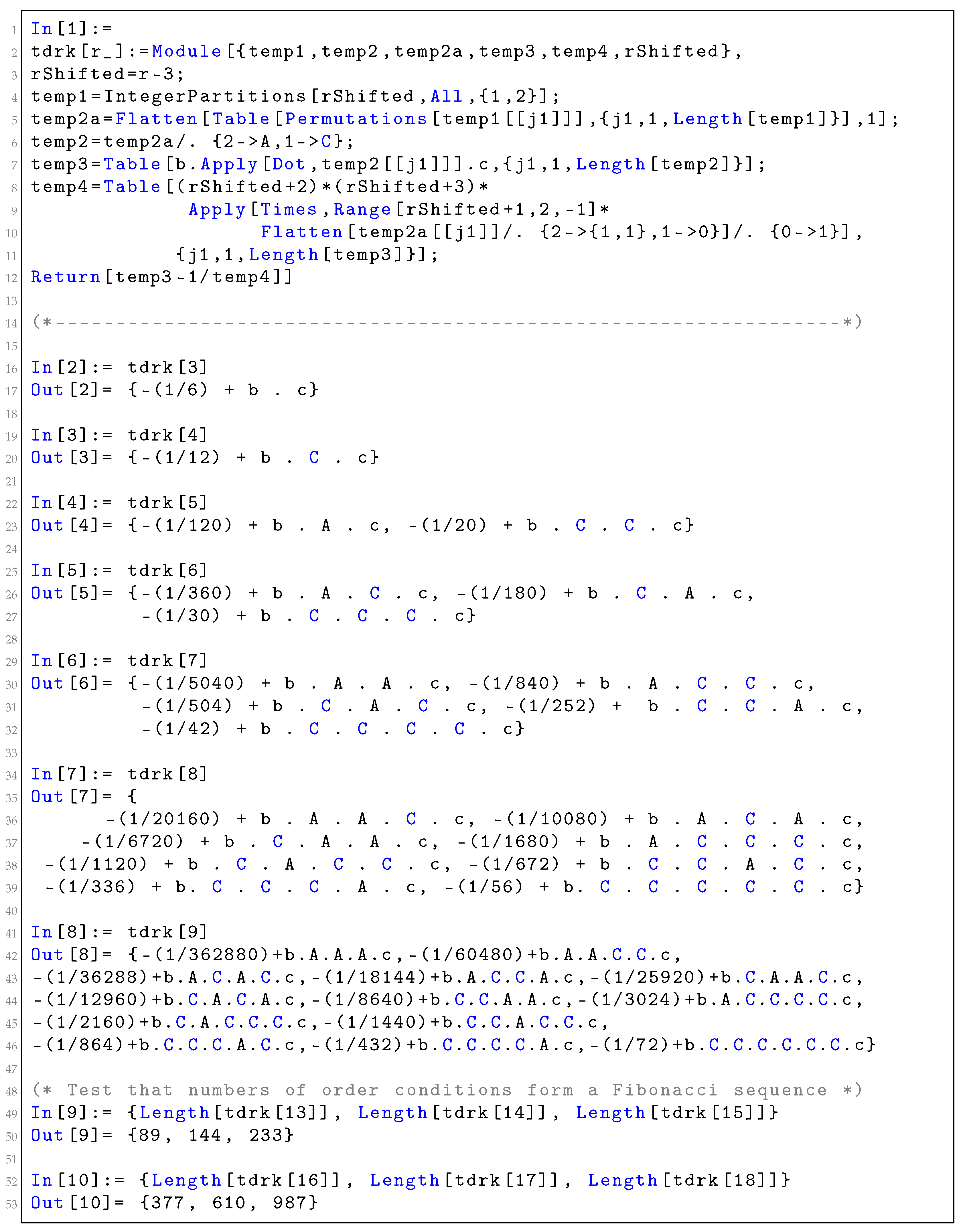
In previous work, we have presented Mathematica [13] programs for deriving order conditions for various related methods. In Listing 1, we provide a Mathematica function that generates the order conditions for the methods under consideration. Only the equation of second order ( b · e = 1 2 ) cannot be derived by this function. The first order is automatically satisfied since the formula of these methods incorporates the Euler method,
y n + 1 = y n + h f ( y n ) +
Listing 1. Mathematica function producing the equations of the condition and a list of them through the ninth order.
Mathematics 13 03676 i001
In Listing 1, except for deriving the body of the equations, we may also produce the ratio that is usually present in these type of Runge–Kutta terms as shown there. Variable temp4 is used for delivering this number.
The variable temp4 in the tdrk[n_] function computes a list of denominators, one for each symbolic term in temp3 (i.e., the body of each equation explained above), which are later used to form the subtracted fractions. Each entry in temp4 corresponds to a rational weight of the form 1 d i , where d i is a combinatorial factor derived from the structure of the corresponding operator sequence.
For a given input r, let r 3 = r 3 . Then:
  • Let q i be the i-th operator sequence, originally derived from a permutation of a composition of r 3 into 1s and 2s.
  • Each 2 (mapped to A) is replaced by {1,1}, and each 1 (mapped to C) is replaced by 0.
  • All 0s are then mapped to 1. The result is a list of 1s, whose length reflects the “weight” or “multiplicity” of the term.
The denominator d i for each term is computed as:
d i = ( r 3 + 2 ) ( r 3 + 3 ) × j = 1 ( r 3 + 2 j ) · w j
where:
  • is the length of the operator sequence q i ,
  • w j are the weights from the transformed sequence described above,
  • The product j ( r 3 + 2 j ) corresponds to a descending factorial (e.g., 4 · 3 · 2 when r 3 = 3 ),
  • The weights w j are all 1s, but repeated depending on the number of 2s in the original partition.
It follows that temp4 evaluates a modified factorial term scaled by a universal prefactor ( r 3 + 2 ) ( r 3 + 3 ) , adjusted for the structure of each term. The final expressions are:
temp 3 1 temp 4 .
in Mathematica notation. Observe that for r = 7 , r 3 = 4 we obtain temp4 = {5040, 840, 504, 252, 42}, and thus, taking into account the body of the terms given above, the five terms of the seventh order shown in Listing 1 are formed.

3. Derivation of the New Pair

We aim to construct a six-stage ( s = 6 ) pair of orders seven and five that satisfies the FSAL (First Same As Last) property, i.e.,  c 6 = 1 , b i = a 6 i , i = 1 , 2 , , 5 . Under this configuration, the final stage (i.e., g 6 ) can be reused as the first stage in the subsequent integration step. Consequently, the number of g-evaluations per step is effectively reduced to five. Including the initial evaluation of f ( y n ) in the summation, the total number of function evaluations per step remains six.
The resulting system of order conditions comprises eighteen equations in total: thirteen corresponding to the seventh-order formula and five to the fifth-order one, i.e.,  b ^ · e = 1 2 , b ^ · c = 1 6 , etc.
By imposing the constraints c 5 = c 6 = 1 , assuming
A · e = 1 2 C · c ,
and enforcing
b ^ 6 = 1 20 b 6 = 0 ,
we may use c 3 and c 4 as free parameters. The remaining order conditions can then be solved in terms of c 3 and c 4 , leading to a consistent solution. Explicitly,
c 2 = 4 7 c 3 7 c 4 + 14 c 3 c 4 7 14 c 3 14 c 4 + 35 c 3 c 4
b 1 = 1 6 c 4 + 7 c 4 2 + c 3 ( 6 + 52 c 4 70 c 4 2 ) + 7 c 3 2 ( 1 10 c 4 + 15 c 4 2 ) 60 c 3 c 4 ( 4 7 c 4 + 7 c 3 ( 1 + 2 c 4 ) ) ,
b 2 = 2401 ( 1 2 c 4 + c 3 ( 2 + 5 c 4 ) ) 5 60 ( 4 7 c 4 + 7 c 3 ( 1 + 2 c 4 ) ) ( 3 7 c 4 + 7 c 3 ( 1 + 3 c 4 ) ) × × ( 4 + c 3 ( 14 28 c 4 ) + 7 c 4 + 7 c 3 2 ( 2 + 5 c 4 ) ) ( 7 c 3 ( 1 4 c 4 + 5 c 4 2 ) 2 ( 2 7 c 4 + 7 c 4 2 ) )
b 3 = 1 6 c 4 + 7 c 4 2 60 ( 1 + c 3 ) c 3 ( c 3 c 4 ) ( 4 + c 3 ( 14 28 c 4 ) + 7 c 4 + 7 c 3 2 ( 2 + 5 c 4 ) ) ,
b 4 = 1 6 c 3 + 7 c 3 2 60 ( 1 + c 4 ) c 4 ( c 3 + c 4 ) ( 7 c 3 ( 1 4 c 4 + 5 c 4 2 ) 2 ( 2 7 c 4 + 7 c 4 2 ) ) ,
b 5 = 2 8 c 4 + 7 c 4 2 + c 3 ( 8 + 37 c 4 35 c 4 2 ) + 7 c 3 2 ( 1 5 c 4 + 5 c 4 2 ) 60 ( 1 + c 3 ) ( 1 + c 4 ) ( 3 7 c 4 + 7 c 3 ( 1 + 3 c 4 ) ) ,
b ^ 1 = 1 + 6 c 4 7 c 4 2 7 c 3 2 ( 1 4 c 4 + 3 c 4 2 ) + c 3 ( 6 28 c 4 + 28 c 4 2 ) 30 c 3 c 4 ( 4 7 c 4 + 7 c 3 ( 1 + 2 c 4 ) ) ,
b ^ 2 = 343 ( 1 2 c 4 + c 3 ( 2 + 5 c 4 ) ) 3 ( 10 46 c 4 + 49 c 4 2 + c 3 ( 46 + 234 c 4 266 c 4 2 ) + 7 c 3 2 ( 7 38 c 4 + 46 c 4 2 ) ) 60 ( 4 7 c 4 + 7 c 3 ( 1 + 2 c 4 ) ) ( 3 7 c 4 + 7 c 3 ( 1 + 3 c 4 ) ) × × ( 4 + c 3 ( 14 28 c 4 ) + 7 c 4 + 7 c 3 2 ( 2 + 5 c 4 ) ) ( 7 c 3 ( 1 4 c 4 + 5 c 4 2 ) 2 ( 2 7 c 4 + 7 c 4 2 ) ) ,
b ^ 3 = ( 2 18 c 3 + 21 c 3 2 ) ( 1 6 c 4 + 7 c 4 2 ) 60 ( 1 + c 3 ) c 3 ( c 3 c 4 ) ( 4 + c 3 ( 14 28 c 4 ) + 7 c 4 + 7 c 3 2 ( 2 + 5 c 4 ) ) ,
b ^ 4 = ( 1 6 c 3 + 7 c 3 2 ) ( 2 18 c 4 + 21 c 4 2 ) 60 ( c 3 c 4 ) ( 1 + c 4 ) c 4 ( 7 c 3 ( 1 4 c 4 + 5 c 4 2 ) 2 ( 2 7 c 4 + 7 c 4 2 ) ) ,
b ^ 5 = 2 + 8 c 4 7 c 4 2 7 c 3 2 ( 1 5 c 4 + 5 c 4 2 ) + c 3 ( 8 37 c 4 + 35 c 4 2 ) 12 ( 1 + c 3 ) ( 1 + c 4 ) ( 3 7 c 4 + 7 c 3 ( 1 + 3 c 4 ) ) ,
a 32 = c 3 ( 4 + 7 c 4 ) ( 1 2 c 4 + c 3 ( 2 + 5 c 4 ) ) ( 4 + c 3 ( 14 28 c 4 ) + 7 c 4 + 7 c 3 2 ( 2 + 5 c 4 ) ) 6 ( 1 6 c 4 + 7 c 4 2 ) ( 4 7 c 4 + 7 c 3 ( 1 + 2 c 4 ) ) ,
a 42 = c 4 ( 1 2 c 4 + c 3 ( 2 + 5 c 4 ) ) × × 16 42 c 4 + 21 c 4 2 + 49 c 3 3 ( 2 + 5 c 4 ) 7 c 3 2 ( 19 + 44 c 4 ) 7 c 3 ( 10 23 c 4 + 4 c 4 2 ) × × 7 c 3 ( 1 4 c 4 + 5 c 4 2 ) 2 ( 2 7 c 4 + 7 c 4 2 ) 6 ( 1 6 c 3 + 7 c 3 2 ) ( 4 7 c 4 + 7 c 3 ( 1 + 2 c 4 ) ) ( 4 + c 3 ( 14 28 c 4 ) + 7 c 4 + 7 c 3 2 ( 2 + 5 c 4 ) )
a 43 = ( c 3 c 4 ) c 4 2 3 c 4 + c 3 ( 3 + 4 c 4 ) 7 c 3 ( 1 4 c 4 + 5 c 4 2 ) 2 ( 2 7 c 4 + 7 c 4 2 ) 6 c 3 ( 1 6 c 3 + 7 c 3 2 ) 4 + c 3 ( 14 28 c 4 ) + 7 c 4 + 7 c 3 2 ( 2 + 5 c 4 ) ,
a 52 = 1 2 c 4 + c 3 ( 2 + 5 c 4 ) · ( 81 1155 c 4 + 5551 c 4 2 12103 c 4 3 + 12348 c 4 4 4802 c 4 5 + 2401 c 3 5 2 + 29 c 4 156 c 4 2 + 396 c 4 3 480 c 4 4 + 225 c 4 5 343 c 3 4 33 + 481 c 4 2553 c 4 2 + 6327 c 4 3 7434 c 4 4 + 3360 c 4 5 + 7 c 3 147 + 2105 c 4 10372 c 4 2 + 23338 c 4 3 24647 c 4 4 + 9947 c 4 5 + 49 c 3 3 215 + 3130 c 4 16284 c 4 2 + 39206 c 4 3 44541 c 4 4 + 19404 c 4 5 14 c 3 2 341 + 4930 c 4 24997 c 4 2 + 58226 c 4 3 63798 c 4 4 + 26754 c 4 5 ) 6 · 4 7 c 4 + 7 c 3 ( 1 + 2 c 4 ) · 4 + c 3 ( 14 28 c 4 ) + 7 c 4 + 7 c 3 2 ( 2 + 5 c 4 ) · 2 8 c 4 + 7 c 4 2 + c 3 ( 8 + 37 c 4 35 c 4 2 ) + 7 c 3 2 ( 1 5 c 4 + 5 c 4 2 ) · 7 c 3 ( 1 4 c 4 + 5 c 4 2 ) 2 ( 2 7 c 4 + 7 c 4 2 )
a 53 = ( 1 + c 3 ) ( 3 + 22 c 4 65 c 4 2 + 91 c 4 3 49 c 4 4 + 7 c 3 3 ( 3 13 c 4 + 12 c 4 2 ) + c 3 2 ( 30 + 145 c 4 238 c 4 2 + 238 c 4 3 147 c 4 4 ) + c 3 ( 16 98 c 4 + 251 c 4 2 343 c 4 3 + 196 c 4 4 ) ) 6 c 3 ( c 3 c 4 ) 4 + c 3 ( 14 28 c 4 ) + 7 c 4 + 7 c 3 2 ( 2 + 5 c 4 ) · 2 8 c 4 + 7 c 4 2 + c 3 ( 8 + 37 c 4 35 c 4 2 ) + 7 c 3 2 ( 1 5 c 4 + 5 c 4 2 )
a 54 = ( 1 + c 3 ) ( 1 6 c 3 + 7 c 3 2 ) ( 1 + c 4 ) 2 3 7 c 4 + 7 c 3 ( 1 + 3 c 4 ) 6 c 4 · ( 49 c 3 4 ( 1 9 c 4 + 30 c 4 2 45 c 4 3 + 25 c 4 4 ) 2 c 4 ( 4 30 c 4 + 84 c 4 2 105 c 4 3 + 49 c 4 4 ) + 7 c 3 3 ( 12 96 c 4 + 264 c 4 2 255 c 4 3 70 c 4 4 + 175 c 4 5 ) + c 3 ( 8 14 c 4 204 c 4 2 + 903 c 4 3 1386 c 4 4 + 735 c 4 5 ) c 3 2 ( 46 288 c 4 + 392 c 4 2 + 805 c 4 3 2520 c 4 4 + 1715 c 4 5 ) )
and
a j 1 = c j 2 / 2 k = 2 j 1 a j k , j = 2 , 3 , , s .
We choose
c 3 = 3 7 and c 4 = 3 4 .
The corresponding method coefficients are reported in Table 2. With this choice, the infinity norm for order conditions of order eight (which govern the leading error terms) is approximately 2.8 × 10 5 , which is considered a relatively small value. This minimization is a standard technique in the literature of numerical ODEs [6,14]. The selection of the free parameters requires careful attention. For instance, if one selects c 3 = 1 100 and c 4 = 5 22 , the maximum absolute norm increases to approximately 0.1 , that is, nearly four orders of magnitude greater. In such a case, the benefits achieved through higher-order accuracy are effectively lost due to this suboptimal choice.
When using the proposed method with stepsize control Formula (1), we set p = 7 , q = 5 .
The stability function of the above STDRK method is given by
R ( z ) = 1 + z w I s z A ^ z 2 A 1 e + z 2 b I s z A ^ z 2 A 1 e
with
A ^ = 0 0 0 0 0 0 1 7 0 0 0 0 0 3 7 0 0 0 0 0 3 4 0 0 0 0 0 1 0 0 0 0 0 1 0 0 0 0 0 .
and w = ( 1 , 0 , 0 , 0 , 0 , 0 ) .
The stability region (i.e., when | R ( z ) | 1 ) of the seventh order method presented here along with the corresponding region for RKPT75 given in [6] is shown in Figure 1.

4. Numerical Tests

We chose three pairs for comparisons. Namely,
  • RKPT7(5), a nine-stage pair presented in [6].
  • DP5(4), the almost classical six-stage FSAL pair due to Dormand and Prince [14].
  • STDRK7(5), the five-plus one-stage FSAL pair proposed in this study.
The orders of the pairs follow their names.
In [5], a pair of methods of orders seven and six is presented. However, the associated error estimator is defective. The sixth-order method satisfies three of the order conditions required for seventh-order accuracy, e.g.,  b ^ · c 5 = 1 42 , among others, and therefore often exhibits seventh-order behavior in practice for many problems. As a result, the local error estimation becomes unreliable, making effective step size control impossible. Consequently, this method was not considered for testing in [5], and it is similarly excluded from the present analysis.
All methods were run in MATLAB [15] with tolerances τ = 10 5 , 10 6 , 10 7 , 10 8 , 10 9 . The ode45 function in MATLAB was used for the DP5(4) pair, while the stdrk75 function, listed in Appendix A, was employed for the new pair introduced in this work. A similar MATLAB implementation to that provided in [16] was used for RKPT7(5). The results are presented as efficiency curves, depicting the number of stages required versus the accuracy achieved. CPU times are not reported, as they can be significantly affected by differences in programming style and implementation details. In contrast, the number of stages depends solely on the underlying method and therefore provides a more objective measure of efficiency.
The problems tested are the following [5,17].
Prothero-Robinson Problem: The ordinary differential equation under consideration is
y ( x ) = ξ ( y ( x ) ζ ( x ) ) + ζ ( x ) , y ( 0 ) = ζ ( 0 ) , ξ < 0 ,
where ζ ( x ) is a sufficiently smooth function; see Example 1 in both [18,19]. The exact solution to this problem is given by y ( x ) = ζ ( x ) . In our numerical experiments, we selected ζ ( x ) = sin x and integrated up to 10 π . Initially, we note that
y ( x ) = ξ 2 ( y ( x ) ζ ( x ) ) + ζ ( x ) = ξ 2 y ( x ) ( ξ 2 + 1 ) sin ( x ) .
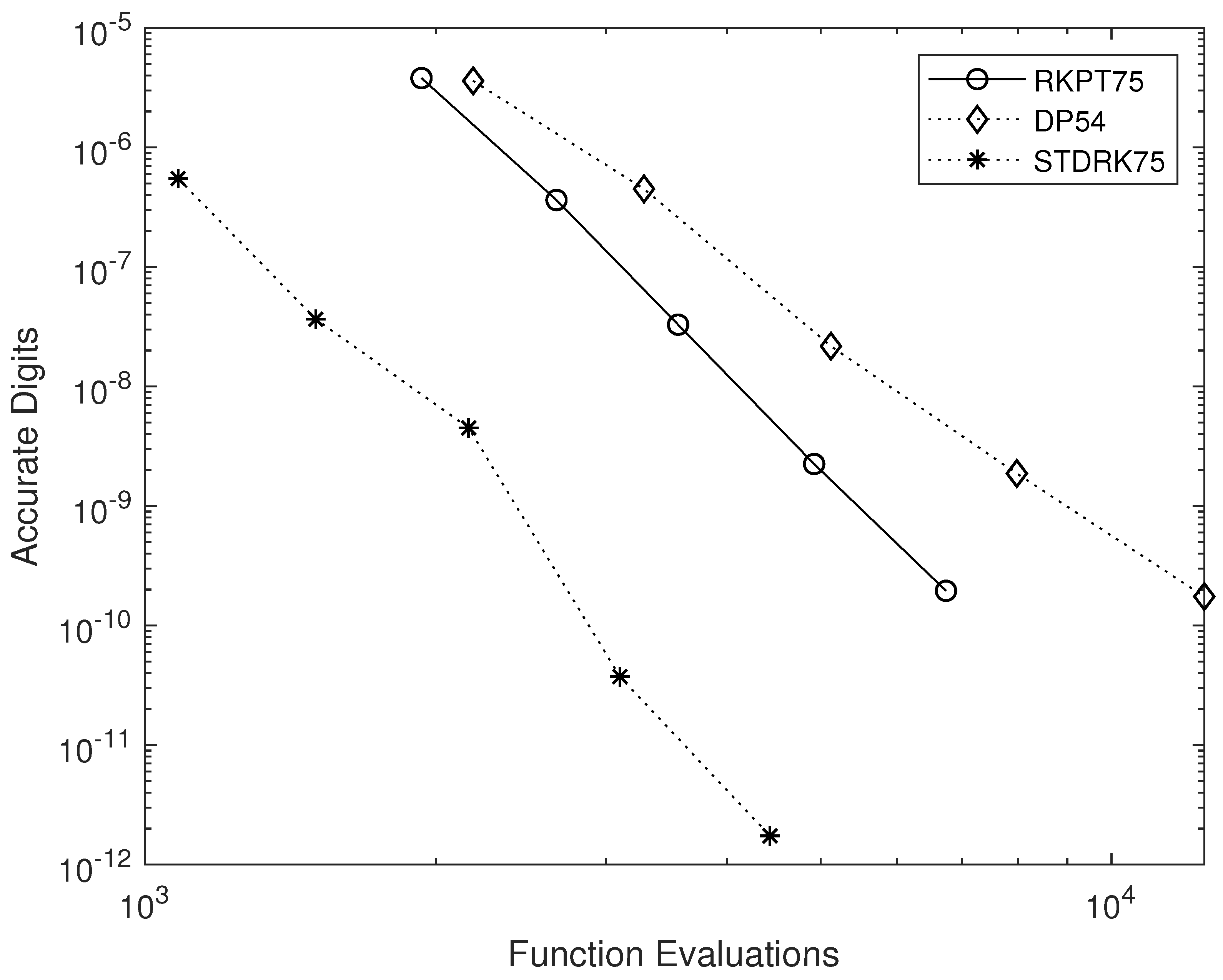
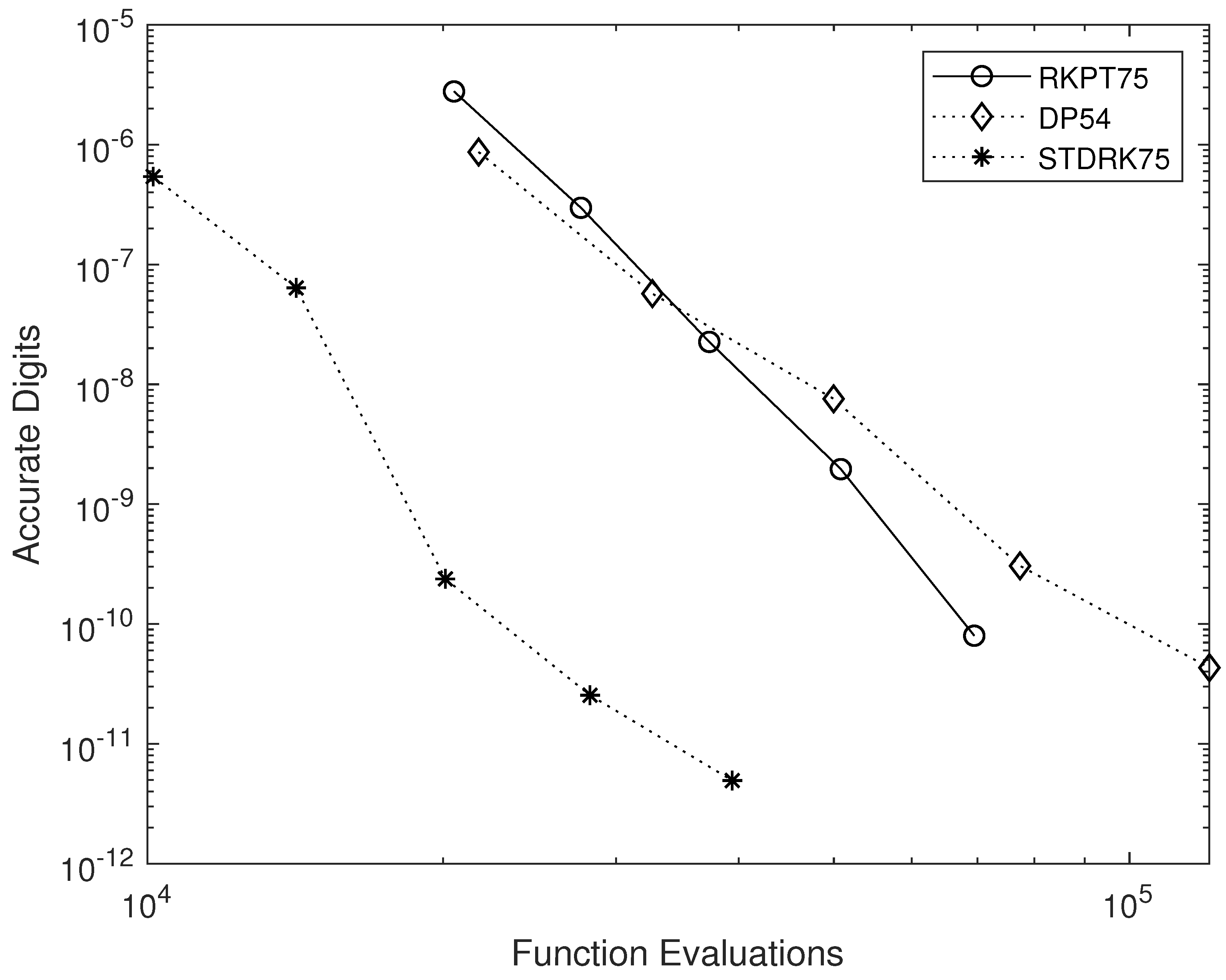
Results are presented for two distinct values of ξ , specifically, 10 and 200 . Both in the non-stiff problem (i.e., ξ = 10 ) and under mild stiffness (i.e., ξ = 200 ), our method demonstrates a clear advantage. As illustrated in Figure 2, STDRK7(5) outperforms RKPT7(5) and DP5. Furthermore, Figure 3 highlights that the STDRK pair achieves higher efficiency compared to other Runge–Kutta pairs.
We further extended our tests to larger magnitudes of ξ , specifically, 500 , 1000 , and  2000 , and observed consistent behavior and comparable results to the ξ = 200 case. These outcomes suggest that, for the Prothero–Robinson problem, the STDRK pair generally offers superior efficiency relative to classical Runge–Kutta methods.
Kaps Problem: The system of differential equations is
y ( x ) = y 1 ( 1 + y 1 ) + y 2 ξ ( y 1 2 y 2 ) 2 y 2 , y ( 0 ) = 1 1 ,
where ξ is a positive parameter. The exact solution is
y ( x ) = exp ( x ) exp ( 2 x ) .
It is a variant of a problem given in [20]. The second derivative is
y ( x ) = y 1 + ( 3 + ξ ) y 1 2 + 2 y 1 3 ( ξ + 3 ) y 2 2 y 1 y 2 ( 4 ξ + ξ 2 ) y 1 2 2 ξ y 1 3 + 2 ξ y 1 y 2 + ( ξ + 2 ) 2 y 2 .
Numerical results are provided in Figure 4 and Figure 5 for two representative values of ξ , specifically, 10 and 200, corresponding to moderately and significantly stiff problems, respectively. In both cases, the proposed pair exhibits a clear performance advantage, consistently achieving higher accuracy and efficiency when compared to the other embedded pairs considered in this study.
Two body problem: We also considered the Kepler problem
y ( x ) = y 3 ( x ) y 4 ( x ) y 1 ( x ) r 3 y 2 ( x ) r 3 .
with second derivative
y ( x ) = y 1 y 2 y 3 y 4 = y 1 r 3 y 2 r 3 r 2 y 3 3 y 1 ( y 1 y 3 + y 2 y 4 ) r 5 r 2 y 4 3 y 2 ( y 1 y 3 + y 2 y 4 ) r 5 ,
where r = y 1 2 + y 2 2 . The integration interval chosen is [ 0 , 100 π ] , and the initial values were
y 1 ( 0 ) = 1 10 , y 2 ( 0 ) = y 3 ( 0 ) = 0 , y 4 ( 0 ) = 19 ,
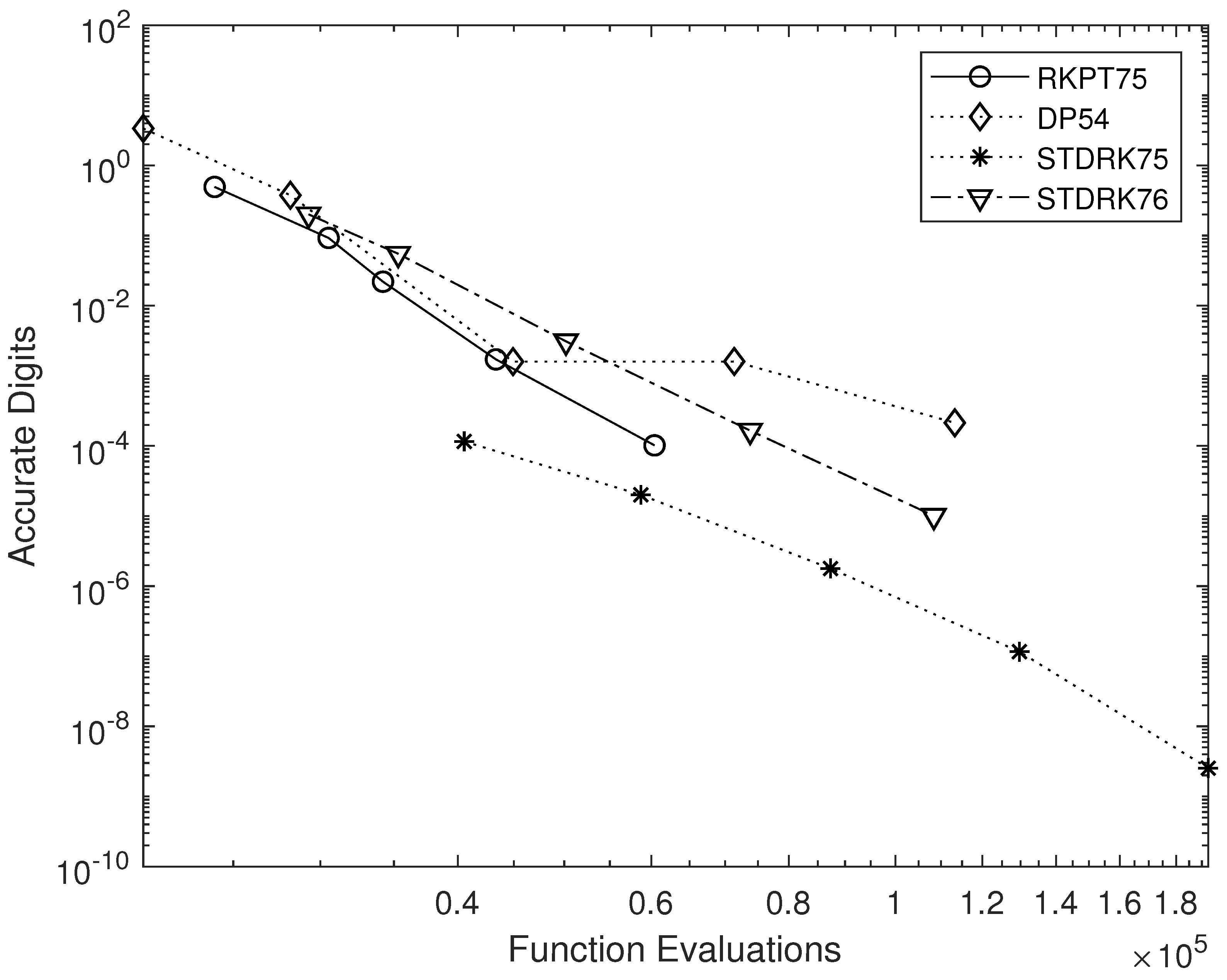
i.e., an orbit with eccentricity 9 10 . In the tests, we included the STDRK7(6) pair described in [5]. The efficiency curves (number of stages versus accuracy) are presented in Figure 6, once again demonstrating the superiority of the new pair proposed in this work.
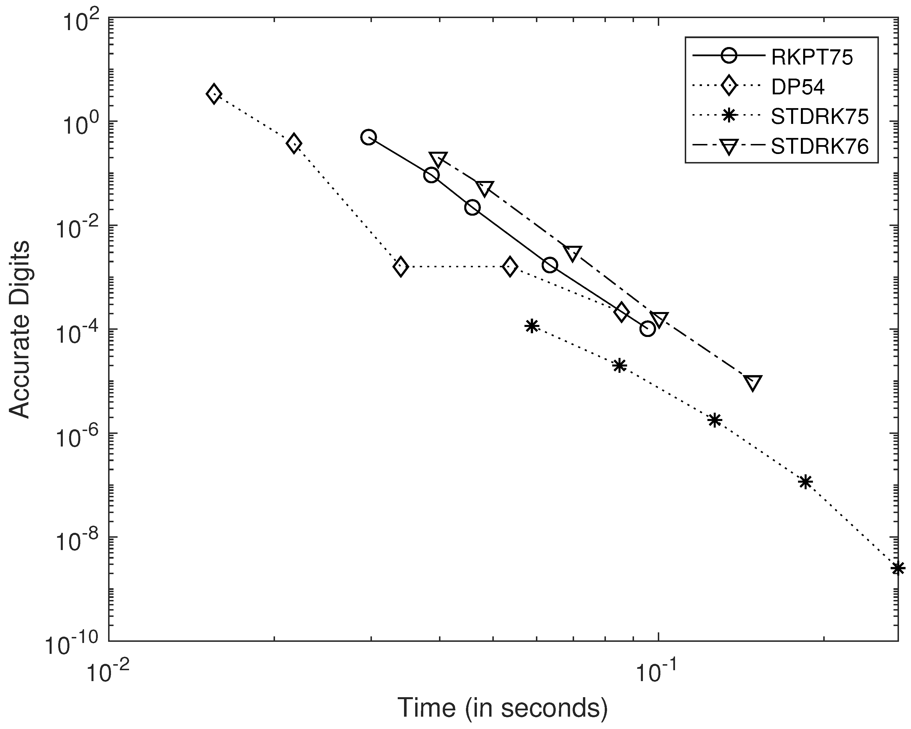
It should be noted that CPU timing is a somewhat misleading performance metric, as it depends heavily on factors such as programming technique, the hardware used, and the software environment (e.g., MATLAB, Python), where built-in functions (such as ode45) often have an inherent advantage. Nevertheless, we present timing results for the Kepler problem in Figure 7. Although ode45 benefits from being a system-optimized function, our proposed method still maintains a performance lead.

5. Conclusions

This work presents a new family of explicit special two-derivative Runge–Kutta (STDRK) pairs, emphasizing seventh-order accuracy with embedded fifth-order control for efficient integration of ordinary differential equations. By leveraging the availability of the second derivative y = f ( y ) f ( y ) , the proposed methods achieve a notable reduction in function evaluations per step. The algebraic construction framework enables a systematic derivation of order conditions, while the accompanying Mathematica implementation supports easy extensibility and exploration of new schemes.
Key contributions include:
  • High-order accuracy: Development of seventh-order STDRK pairs with embedded fifth-order error control.
  • Computational efficiency: Significant reduction in function evaluations through the use of second-derivative information.
  • Practical framework: Provision of a symbolic construction and verification tool in Mathematica.
Numerical experiments confirm the theoretical expectations, showing favorable performance compared to established methods. These results indicate that STDRK schemes offer a promising direction for accurate and efficient integration of both stiff and non-stiff problems.

Author Contributions

Conceptualization, I.A., T.E.S. and C.T.; Methodology, T.E.S. and C.T.; Software, I.A., T.E.S. and C.T.; Validation, I.A., T.E.S. and C.T.; Formal analysis, I.A., T.E.S. and C.T.; Investigation, I.A., T.E.S. and C.T.; Resources, I.A., T.E.S. and C.T.; Data curation, I.A., T.E.S. and C.T.; Writing—original draft, C.T.; Writing—review and editing, T.E.S.; Visualization, I.A., T.E.S. and C.T.; Supervision, T.E.S.; Project administration, T.E.S.; Funding acquisition, I.A. The contributions of all authors to this work are equal. All authors have read and agreed to the published version of the manuscript.

Funding

This work was supported and funded by the Ongoing Research Funding Program (ORF-2025-1246) King Saud University, Riyadh, Saudi Arabia.

Institutional Review Board Statement

Not applicable.

Informed Consent Statement

Not applicable.

Data Availability Statement

The original data and software presented in the study are openly available in http://users.uoa.gr/~tsitourasc/stdrk75.m (accessed on 10 November 2025).

Conflicts of Interest

The authors declare no conflicts of interest.

Appendix A

We present a MATLAB function that presents the coefficients of the new method. The pair is implemented in the way described in the following listing.
function [tout, yout, ireject] = stdrk75(fcn, gcn, t0, tfinal, y0, tol)
% SDRK75: Second-derivative explicit Runge-Kutta method (7th/5th order)
% Solves y’ = f(y), y’’ = f’(y) * f(y) = g(y)
% Inputs:
%   fcn  - function handle for f(y)
%   gcn  - function handle for g(y)
%   t0   - initial time
%   tfinal - final time
%   y0   - initial condition
%   tol  - tolerance for adaptive step size
% Outputs:
%   tout - time values
%   yout - solution values
%   ireject - number of rejected steps
% Coefficients
a=[  000000;
1/9800000;
-1/985/490000;
169/1024-119/2048357/2048000;
-29/18231/85-112/135512/229500;
11/2702401/122402401/12960512/68851/2880]’;
b=[11/270, 2401/12240, 2401/12960, 512/6885, 1/288, 0];
bb=[53/270, -(343/2448), 6517/12960, -832/6885, -11/288, 1/10];
c=[0, 1/7, 3/7, 3/4, 1, 1]’;
% Initialization
t = t0;
y = y0(:);
s = length(c);
g = zeros(length(y), s);
 
% Estimate initial step size
f = fcn(y);
pow = 1/7;
h = tol^pow / max(max(abs(f)), 1e-2);
hmax = (tfinal - t) / 5;
hmin = (tfinal - t) / 2e6;
h = min(hmax, max(h, hmin));
 
% Preallocate output buffers (initial guess)
max_steps = ceil((tfinal - t0) / hmin);
tout = zeros(max_steps, 1);
yout = zeros(max_steps, length(y));
tout(1) = t;
yout(1, :) = y.’;
step = 1;
 
% Initial second derivative
g(:,1) = gcn(y);
ireject = 0;
% Main integration loop
while t < tfinal && h >= hmin
    if t + h > tfinal
       h = tfinal - t;
    end
 
    % Compute g at intermediate stages
    for j = 2:s
       y_stage = y + c(j)*h*f + h^2 * g * a(:,j);
       g(:,j) = gcn(y_stage);
    end
 
    % Error estimation (embedded method)
    delta = norm(h * g * (b - bb)’, inf)^(1.1666);
 
    if delta <= tol
       % Accept step
       t = t + h;
       y = y + h * f + h^2 * g * b’;
       f = fcn(y);             % next step’s f
       g(:,1) = g(:,s);          % FSAL: reuse last g
       step = step + 1;
       tout(step) = t;
       yout(step, :) = y.’;
    else
       ireject = ireject + 1;
    end
 
    % Adjust step size
    if delta ~= 0
       h = min(hmax, 0.8 * h * (tol / delta)^pow);
    end
end
 
% Trim unused preallocated space
tout = tout(1:step);
yout = yout(1:step, :);
 
% Warn if failed
if t < tfinal
   warning(’Singularity likely. Integration stopped at t = %g.’, t);
end
end
%--------------------------------------------------------------------
          A sample run for the Kaps problem with ξ = 200 and δ = 10 9 could be
>> xi=200;
[tout, yout, ireject] = stdrk75(@(y) [-y(1)*(1+y(1))+y(2); ...
                  xi*(y(1)^2-y(2))-2*y(2)], ...
   @(y) [y(1)+(3 + xi)*y(1)^2+2*y(1)^3-(xi + 3)*y(2)-2*y(1)*y(2);    ...
   -(4*xi+xi^2)*y(1)^2-2*xi*y(1)^3+2*xi*y(1)*y(2)+(xi + 2)^2*y(2)],  ...
   0, 10*pi, [1 1]’,  1e-9);
fprintf(’stages=%6.0f\n’, length(tout)*6 + ireject*5);
fprintf(’max abs error=%9.2e\n’, ...
     max(max(abs(yout - [exp(-tout) exp(-2*tout)]))));
 
stages= 11073
max abs error= 7.72e-10
           This result corresponds to the rightmost lowest star in Figure 4.

References

  1. Butcher, J.C. Numerical Methods for Ordinary Differential Equations; Wiley: Chichester, UK, 2008. [Google Scholar]
  2. Famelis, I.T.; Tsitouras, C. Symbolic derivation of order conditions for hybrid Numerov-type methods solving y=f(x,y). J. Comput. Appl. Math. 2008, 218, 543–555. [Google Scholar] [CrossRef]
  3. Iserles, A. A First Course in the Numerical Analysis of Differential Equations; Cambridge University Press: Cambridge, UK, 2009. [Google Scholar]
  4. Simos, T.E.; Tsitouras, C. Evolutionary derivation of Runge–Kutta pairs for addressing inhomogeneous linear problems. Numer. Algorithms 2021, 87, 511–525. [Google Scholar] [CrossRef]
  5. Chan, R.P.K.; Tsai, A.Y.J. On explicit two-derivative Runge–Kutta methods. Numer. Algorithms 2010, 53, 171–194. [Google Scholar] [CrossRef]
  6. Tsitouras, C.; Papakostas, S.N. Cheap Error Estimation for Runge–Kutta Methods. SIAM J. Sci. Comput. 1999, 20, 2067–2088. [Google Scholar] [CrossRef]
  7. Abdulsalam, A.; Senu, N.; Majid, Z.A.; Asri, N.M.; Long, N. Adaptive multi-step Runge–Kutta–Nyström methods for general second-order ordinary differential equations. J. Comput. Appl. Math. 2023, 421, 114874. [Google Scholar] [CrossRef]
  8. Fekete, I.; Conde, S.; Shadid, J.N. Embedded pairs for optimal explicit strong stability preserving Runge–Kutta methods. J. Comput. Appl. Math. 2022, 401, 114325. [Google Scholar] [CrossRef]
  9. Hairer, E.; Nørsett, S.P.; Wanner, G. Solving Ordinary Differential Equations I: Nonstiff Problems; Springer: Berlin/Heidelberg, Germany, 1993. [Google Scholar]
  10. Xu, X.; Li, B. Semi-global stabilization of parabolic PDE–ODE systems with input saturation. Automatica 2025, 121, 111931. [Google Scholar] [CrossRef]
  11. Bo, Y.; Tian, D.; Liu, X.; Jin, Y.F. Discrete Maximum Principle and Energy Stability of the Compact Difference Scheme for Two-Dimensional Allen-Cahn Equation. J. Funct. Spaces 2022, 2022, 8522231. [Google Scholar] [CrossRef]
  12. Huang, Z.-Y.; Zheng, X.-Q.; Li, C.; Tan, E.L.; Chen, Z.-A.; Shi, L.-H. Piecewise Calculation Scheme for the Unconditionally Stable Chebyshev Finite-Difference Time-Domain Method. IEEE Trans. Microw. Theory Tech. 2025, 73, 4588–4596. [Google Scholar] [CrossRef]
  13. Wolfram Research, Inc. Mathematica, Version 13.3; Wolfram Research, Inc.: Champaign, IL, USA, 2023.
  14. Dormand, J.R.; Prince, P.J. A family of embedded Runge–Kutta formulae. J. Comput. Appl. Math. 1980, 6, 19–26. [Google Scholar] [CrossRef]
  15. The MathWorks, Inc. MATLAB, Version R2024b; The MathWorks, Inc.: Natick, MA, USA, 2024.
  16. Tsitouras, C. Explicit Runge–Kutta pairs appropriate for engineering applications. Appl. Math. Model. 2002, 26, 77–88. [Google Scholar] [CrossRef]
  17. Turaci, M.O.; Öziş, T. On explicit two-derivative two-step Runge–Kutta methods. Comput. Appl. Math. 2018, 37, 6920–6945. [Google Scholar] [CrossRef]
  18. Prothero, A.; Robinson, A. On the stability and accuracy of one-step methods for solving stiff systems of ordinary differential equations. Math. Comput. 1974, 28, 145–162. [Google Scholar] [CrossRef]
  19. Seinfeld, J.H.; Lapidus, L.; Hwang, M. Review of numerical integration techniques for stiff ordinary differential equations. Ind. Eng. Chem. Fundam. 1970, 9, 266–275. [Google Scholar] [CrossRef]
  20. Dekker, K.; Verwer, J.G. Stability of Runge–Kutta Methods for Stiff Nonlinear Differential Equations; North-Holland: Amsterdam, The Netherlands, 1984. [Google Scholar]
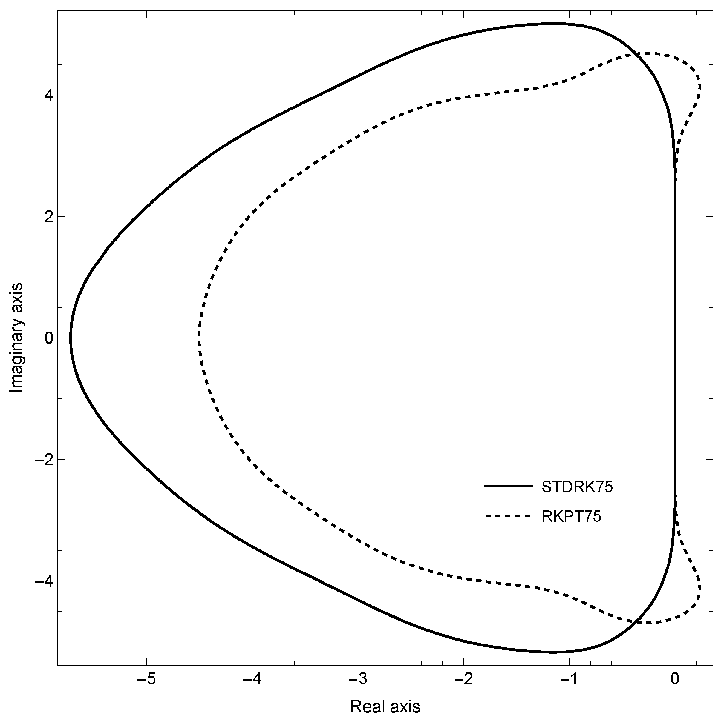
Figure 1. Stability regions.
Mathematics 13 03676 g001
Figure 2. Efficiency curves for the Prothero–Robinson problem and ξ = 10 .
Mathematics 13 03676 g002
Figure 3. Efficiency curves for the Prothero–Robinson problem and ξ = 200 .
Mathematics 13 03676 g003
Figure 4. Efficiency curves for the Kaps problem and ξ = 10 .
Mathematics 13 03676 g004
Figure 5. Efficiency curves for the Kaps problem and ξ = 200 .
Mathematics 13 03676 g005
Figure 6. Efficiency curves (stages vs. accuracy) for the Kepler problem with eccentricity 9 10 .
Mathematics 13 03676 g006
Figure 7. Efficiency curves (time vs. accuracy) for the Kepler problem with eccentricity 9 10 .
Mathematics 13 03676 g007
Table 1. Compositions of n 3 with parts 2 and their corresponding Fibonacci numbers.
n n 3 Compositions with Parts 2 F ( n )
30(empty sum)1
4111
521 + 1, 22
631 + 1 + 1, 1 + 2, 2 + 13
741 + 1 + 1 + 1, 1 + 1 + 2, 1 + 2 + 1, 2 + 1 + 1, 2 + 25
85(8 compositions)8
Table 2. The coefficients of the new pair of orders seven and five proposed here.
0
1 7 1 98
3 7 1 98 5 49
3 4 169 1024 119 2048 357 2048
1 29 18 231 85 112 135 512 2295
1 11 270 2401 12240 2401 12960 512 6885 1 288
b 11 270 2401 12240 2401 12960 512 6885 1 288 0
b ^ 53 270 343 2448 6517 12960 832 6885 11 288 1 10
Disclaimer/Publisher’s Note: The statements, opinions and data contained in all publications are solely those of the individual author(s) and contributor(s) and not of MDPI and/or the editor(s). MDPI and/or the editor(s) disclaim responsibility for any injury to people or property resulting from any ideas, methods, instructions or products referred to in the content.