Non-Singular Generalized RBF Solution and Weaker Singularity MFS: Laplace Equation and Anisotropic Laplace Equation

Abstract

This paper introduces a singular distance function r_s in terms of a symmetric non-negative metric tensor S. If S satisfies a quadratic matrix equation involving a parameter β, then for the Laplace equation $r_s^{\beta }$ is a non-singular generalized radial basis function solution if 2 > β > 0, and a weaker singularity fundamental solution if −1 < β < 0. With a unit vector as a medium to express S, we can derive the metric tensor in closed form and prove that S is a singular projection operator. For the anisotropic Laplace equation, the corresponding closed-form representation of S is also derived. The concept of non-singular generalized radial basis function solution for the Laplace-type equations is novel and useful, which has not yet appeared in the literature. In addition, a logarithmic type method of fundamental solutions is developed for the anisotropic Laplace equation. Owing to non-singularity and weaker singularity of the bases of solutions, numerical experiments verify the accuracy and efficiency of the proposed methods.

1. Introduction

Since the work of Kupradze [1], there have appeared numerous discussions of the method of fundamental solutions (MFS) for the purpose of an easy computation of engineering problems. The fundamental solutions for the commonly used linear partial differential equations (PDEs) are listed in text books [2,3]. A review of the MFS for elliptic type PDEs up to 1998 was given in [4]. More topics for the MFS were issued in [5].

It is known that $1/r$ is a fundamental solution of the 3D Laplace equation:

$$\begin{array}{c}\Delta u\left(\mathbf{x}\right)=0,\mathbf{x}\in \mathrm{\Omega }\subset {\mathbb{R}}^3,\hfill \end{array}$$

(1)

$$\begin{array}{c}{u\left(\mathbf{x}\right)|}_{\mathbf{x}\in \Gamma }=f\left(\mathbf{x}\right),\hfill \end{array}$$

(2)

satisfying

$$\Delta {\displaystyle \frac{1}{r}}=\nabla ·\left(\nabla {\displaystyle \frac{1}{r}}\right)=-\nabla ·\left(\nabla {\displaystyle \frac{\mathbf{r}}{r^3}}\right)=\delta \left(\mathbf{r}\right),$$

(3)

where $\delta$ is the Dirac delta function, due to $r^3\to 0$ when $\mathbf{x}\to {\mathbf{x}}^s$; $r=\parallel \mathbf{r}\parallel =\parallel \mathbf{x}-{\mathbf{x}}^s\parallel$, and ${\mathbf{x}}^s$ is a source point. It is evident from Equation (3) that $1/r\left(\mathbf{x}\right)$ is a fundamental solution of Equation (1), whose order of singularity is one. The derivation of Equation (3) is relegated into Appendix A.

In the whole paper the domain $\mathrm{\Omega }$ of the problem considered is supposed to be bounded, and its boundary is continuous and piecewise smooth.

The singularity of MFS occurs as $\mathbf{x}={\mathbf{x}}^s$ where $1/r$ grows to infinity. One of the issues to reduce the ill-posedness due to the singularity is a proper selection of source points to improve the performance of MFS [6,7,8]. Wang et al. [9] proposed a novel adaptive method of fundamental solutions with physics-informed neural networks to determine the source points.

As noted in [3] the functions expressed in terms of the Euclidean distance belong to the radial basis function (RBF). For the linear PDEs the radially symmetric fundamental solutions have the radial form to be radial functions. For this reason Golberg and Chen [10] categorized the MFS into the class of the methods of RBFs. The MFS exhibits singularities at source points, where special treatment of these singularities should be handled numerically. To overcome the singularity of MFS, the RBF general solutions were proposed in [11] for varied orders of the vibrational thin, the Berger, and the Winkler plates, in [12] for the boundary particle method, and in [13,14] for the boundary knot method. These papers proposed non-singular radial functions as the bases of solutions. To further overcome the ill-posedness, there were some discussions on the improvements of the boundary knot method [15,16].

The boundary knot method (BKM) was developed by Chen and Tanaka [12], and it synergistically combines the merits of MFS and RBF techniques. Later many applications of BKM can be seen in the literature, such as the solution of two-dimensional advection reaction–diffusion and Brusselator equations [17], the 2D and 3D Helmholtz and convection–diffusion problems under complicated geometry [18], the inverse problems associated with the Helmholtz equation [19], with fictitious sources for solving Helmholtz-type equations [20], and the modified boundary knot method for multi-dimensional harmonic-type equations [21].

The non-singular RBF general solutions utilized for some commonly used linear PDEs were listed in Table 2.7 of [3]. Unfortunately the non-singular RBF solution for the Laplace equation is a constant, which is not suitable to be the basis of solution. The lack of non-singular RBF solutions for the Laplace-type equations motivates us to develop the non-singular generalized RBF solution (NSGRBF) in the present paper.

Chen et al. [11] used the non-singular RBF solutions of Helmholtz-like equation with a small characteristic parameter to overcome this difficulty. However, when the characteristic parameter should generally be small to get an accurate solution of the Laplace equation, the accuracy of numerical solution is very sensitive to the domain geometry. In this paper we generalize the radial function in terms of a singular distance function $r_s(\mathbf{x},\mathbf{y})=\sqrt{{\mathbf{r}}^T\mathbf{S}\mathbf{r}}$, where $\mathbf{r}=\mathbf{x}-\mathbf{y}$, and $\mathbf{S}\ge \mathbf{0}$ with det$\left(\mathbf{S}\right)=0$ is a singular symmetric tensor. If one takes $\mathbf{S}={\mathbf{I}}_3$, $r_s$ recovers to the usual Euclidean distance function $r(\mathbf{x},\mathbf{y})=\parallel \mathbf{r}\parallel$. $r_s$ possesses the following properties: (i) $r_s(\mathbf{x},\mathbf{y})\ge 0$, (ii) $r_s(\mathbf{x},\mathbf{y})=r_s(\mathbf{y},\mathbf{x})$, and (iii) $r_s(\mathbf{x},\mathbf{z})\le r_s(\mathbf{x},\mathbf{y})+r_s(\mathbf{y},\mathbf{z})$. In addition to these properties, $r(\mathbf{x},\mathbf{y})$ possesses an extra property of $r(\mathbf{x},\mathbf{y})=0$ iff $\mathbf{x}=\mathbf{y}$. This property does not hold for $r_s(\mathbf{x},\mathbf{y})$ because, when $\mathbf{r}\ne 0$ lies in the null space of $\mathbf{S}$, we have $r_s(\mathbf{x},\mathbf{y})=0$ even for $\mathbf{x}\ne \mathbf{y}$.

The new solution in terms of $r_s$ will be called the generalized RBF solution, in contrast to the r-dependent RBF solution. Then we will extend the non-singular generalized RBF solution for the Laplace equation to the anisotropic Laplace equation:

$$\nabla ·[\mathbf{K}\nabla u\left(\mathbf{x}\right)]=0,\mathbf{x}\in \mathrm{\Omega }\subset {\mathbb{R}}^3,$$

(4)

where $\mathbf{K}$ is a positive-definite and symmetric anisotropic tensor.

For the anisotropic Laplace equation, the domain mapping method was derived in [22], and the boundary knot method based on geodesic distance was proposed in [23]. The newly defined generalized RBF solutions can be adopted as alternative and effective bases to find the numerical solutions of the Laplace equation and anisotropic Laplace equation.

The work on generalized operators in [24] can provide insights into extending the RBF framework to more complex approximations. On the other hand the methods for fractional systems in [25] may inspire analogous approaches for singular and non-singular solutions in PDEs.

By applying the MFS to solve the Laplace-type PDEs, it is utmost important, by using the de-singularized technique, to reduce the ill-conditioned behavior and then raise the computational efficiency and accuracy. The novel contributions of the present paper for solving the 3D Laplace equation and anisotropic Laplace equation are summarized as follows:

• The extension from the original MFS to the non-singular generalized RBF (NSGRBF) using the novel bases can be carried out to improve the ill-posedness of the original MFS and enhance the accuracy of numerical solutions.
• The de-singularized technique is simple and efficient.
• The NSGRBF solution bases were derived at the first time for both the Laplace equation and anisotropic Laplace equation.

2. Generalized RBF Solution

The following vector notations can facilitate the proofs of the new results:

$$\mathbf{x}:=\left[\begin{array}{c}x\\ y\\ z\end{array}\right],{\mathbf{x}}^s:=\left[\begin{array}{c}{x}^s\\ y^s\\ z^s\end{array}\right],\mathbf{r}:=\left[\begin{array}{c}x-x^s\\ y-y^s\\ z-z^s\end{array}\right],$$

(5)

where $\mathbf{x}\in \overline{\mathrm{\Omega }}:=\mathrm{\Omega }\cup \Gamma$, and ${\mathbf{x}}^s\in {\overline{\mathrm{\Omega }}}^c:={\mathbb{R}}^3\setminus \overline{\mathrm{\Omega }}$ is a source point. Hence,

$$r\left(\mathbf{x}\right)=\parallel \mathbf{r}\left(\mathbf{x}\right)\parallel =\sqrt{{\mathbf{r}}^T\left(\mathbf{x}\right)\mathbf{r}\left(\mathbf{x}\right)}$$

(6)

is a positive distance function of Euclidean type. We define a singular distance function:

$$r_s\left(\mathbf{x}\right)=\sqrt{{\mathbf{r}}^T\left(\mathbf{x}\right)\mathbf{S}\mathbf{r}\left(\mathbf{x}\right)},$$

(7)

where the $3\times 3$ matrix $\mathbf{S}$ is a symmetric non-negative metric tensor; the subscript s means that $r_s$ is a singular distance function. Later we will prove that $\mathbf{S}$ is a continuous quadratic function of a unit vector.

According to Equation (7), we have

$$\nabla r_s\left(\mathbf{x}\right)={\displaystyle \frac{\mathbf{S}\mathbf{r}\left(\mathbf{x}\right)}{r_s\left(\mathbf{x}\right)}}.$$

(8)

Now we attempt to get rid of the singularity in Equation (3) as follows, which is an extension of Theorem 3 in [26].

Theorem 1. 

For the Laplace equation, if the $3\times 3$ symmetric matrix $\mathbf{S}$ satisfies

$${\mathbf{S}}^2={\displaystyle \frac{tr\left(\mathbf{S}\right)}{2-\beta }}\mathbf{S},$$

(9)

where $tr\left(\mathbf{S}\right)>0$ is the trace of $\mathbf{S}$, then

$$U\left(\mathbf{x}\right)=r_s^{\beta }\left(\mathbf{x}\right)={\left[{\mathbf{r}}^T\left(\mathbf{x}\right)\mathbf{S}\mathbf{r}\left(\mathbf{x}\right)\right]}^{\beta /2}$$

(10)

satisfies Equation (1):

$$\nabla ·[\nabla U(\mathbf{x}\left)\right]=\Delta U\left(\mathbf{x}\right)=0.$$

(11)

When $2>\beta >0$, $U\left(\mathbf{x}\right)$ is a generalized RBF solution without having singularity; when $-1<\beta <0$, $U\left(\mathbf{x}\right)$ is a singular solution with the order of singularity being $-\beta$.

Proof. 

First we clarify the range of $\beta$. $\beta =2$ is a singular point, which leads to the failure of Equation (9); hence, $\beta <2$ is required. In Equation (10), $\beta =0$ renders a constant value of $U=1$, which is not interesting. Therefore, the range of $\beta$ is $2>\beta >0$ for the non-singular solution U in Equation (10). In MFS the singular solution $U=1/r$ has a singularity order $\beta =-1$. For a less singular solution U in Equation (10), we take $\beta >-1$. Therefore, the range of $\beta$ is $-1<\beta <0$ for the singular solution U in Equation (10).

It follows from Equation (10) that

$$\nabla U=\beta r_s^{\beta -1}\nabla r_s.$$

(12)

Then by means of Equations (12) and (8), one has

$$\nabla U=\beta r_s^{\beta -1}\nabla r_s=\beta r_s^{\beta -1}{\displaystyle \frac{\mathbf{S}\mathbf{r}}{r_s}}=\beta r_s^{\beta -2}\mathbf{S}\mathbf{r}.$$

(13)

We have

$$\nabla ·\left(\mathbf{S}\mathbf{r}\right)=\nabla ·\left[\mathbf{S}(\mathbf{x}-{\mathbf{x}}^s)\right]=\nabla ·\left(\mathbf{S}\mathbf{x}\right)=tr\left(\mathbf{S}\right),$$

(14)

because $\mathbf{S}$ is a constant matrix and ${\mathbf{x}}^s$ is a constant vector.

Taking the divergence on both sides of Equation (13) and using Equation (14) yields

$$\begin{array}{c}\nabla ·(\nabla U)=\beta \nabla ·\left(r_s^{\beta -2}\mathbf{S}\mathbf{r}\right)=\beta r_s^{\beta -2}\nabla ·\left(\mathbf{S}\mathbf{r}\right)+\beta (\nabla r_s^{\beta -2})·\left(\mathbf{S}\mathbf{r}\right)\hfill \\ =\beta r_s^{\beta -2}tr\left(\mathbf{S}\right)+\beta (\beta -2)r_s^{\beta -3}\nabla r_s·\left(\mathbf{S}\mathbf{r}\right).\hfill \end{array}$$

(15)

Using Equations (7), (8) and (15)yields

$$\begin{array}{c}\nabla ·(\nabla U)=\beta r_s^{\beta -2}tr\left(\mathbf{S}\right)+\beta (\beta -2)r_s^{\beta -3}{\displaystyle \frac{\mathbf{S}\mathbf{r}}{r_s}}·\left(\mathbf{S}\mathbf{r}\right)\hfill \\ =\beta r_s^{\beta -2}tr\left(\mathbf{S}\right)+\beta (\beta -2)r_s^{\beta -4}{\mathbf{r}}^T{\mathbf{S}}^T\mathbf{S}\mathbf{r}\hfill \\ =\beta r_s^{\beta -2}tr\left(\mathbf{S}\right)+\beta (\beta -2)r_s^{\beta -4}{\mathbf{r}}^T{\mathbf{S}}^2\mathbf{r}\hfill \\ =\beta r_s^{\beta -4}[r_s^{2}tr\left(\mathbf{S}\right)+(\beta -2){\mathbf{r}}^T{\mathbf{S}}^2\mathbf{r}]\hfill \\ =\beta r_s^{\beta -4}{\mathbf{r}}^T\left[tr\left(\mathbf{S}\right)\mathbf{S}-(2-\beta ){\mathbf{S}}^2\right]\mathbf{r},\hfill \end{array}$$

(16)

where ${\mathbf{S}}^T\mathbf{S}={\mathbf{S}}^2$ was used owing to the symmetry of $\mathbf{S}$. If Equation (9) holds, Equation (11) follows immediately. □

Satisfying Equation (9) by $\mathbf{S}$, a generalized RBF solution (10) for $U\left(\mathbf{x}\right)$ of the Laplace equation is obtained. If $\beta >0$, the singularity of $r_s^{\beta }$ is zero; when $-1<\beta <0$, the singularity of $U\left(\mathbf{x}\right)$ with the order $-\beta$ is weaker than $1/r$ of the original MFS as shown in Equation (3). For the special case with $\beta =0$, Equation (10) is a non-sense constant solution. Rather than a constant solution the logarithmic singular solution $U\left(\mathbf{x}\right)=ln{r}_s\left(\mathbf{x}\right)$ was already derived in [26], if we set $\beta =0$ in Equation (9).

Notice that Theorem 1 involves the fundamental solution $1/r\left(\mathbf{x}\right)$ as a special case. Taking $\beta =-1$, $\mathbf{S}={\mathbf{I}}_3$ is a solution of Equation (9). Then $U\left(\mathbf{x}\right)$ in Equation (10) reduces to $U\left(\mathbf{x}\right)=1/r\left(\mathbf{x}\right)$.

Equation (9) is an operator equation as a projective constraint of $\mathbf{S}$. Applying it to any nonzero vector $\mathbf{b}$ we have

$${\mathbf{b}}^T\mathbf{S}\left[\mathbf{S}-{\displaystyle \frac{tr\left(\mathbf{S}\right)}{2-\beta }}{\mathbf{I}}_3\right]\mathbf{b}=0.$$

(17)

Because $\mathbf{S}$ is symmetric, Equation (17) indicates that $\mathbf{S}\mathbf{b}$ is perpendicular to $[\mathbf{S}-{\displaystyle \frac{tr\left(\mathbf{S}\right)}{2-\beta }}{\mathbf{I}}_3]\mathbf{b}$.

Theorem 2. 

No solution of Equation (9) with $\mathbf{S}>\mathbf{0}$ exists. If $\mathbf{a}$ is a unit vector with $\parallel \mathbf{a}\parallel =1$, then

$$\tilde{\mathbf{S}}={\mathbf{I}}_3-\mathbf{a}{\mathbf{a}}^T$$

(18)

satisfies

$${\tilde{\mathbf{S}}}^2=\tilde{\mathbf{S}},$$

(19)

where $\tilde{\mathbf{S}}\ge \mathbf{0}$ with det($\tilde{\mathbf{S}}$) = 0 is a singular projection operator. Moreover, $\mathbf{S}$ with $tr\left(\mathbf{S}\right)>0$ can be derived as follows:

$$\mathbf{S}={\displaystyle \frac{2-\beta }{2}}\tilde{\mathbf{S}}={\displaystyle \frac{2-\beta }{2}}({\mathbf{I}}_3-\mathbf{a}{\mathbf{a}}^T).$$

(20)

Proof. 

We prove the first statement by a contradiction method. If $\mathbf{S}>\mathbf{0}$ then ${\mathbf{S}}^{-1}$ exists. Multiplying both sides of Equation (9) by ${\mathbf{S}}^{-1}$ leads to

$$\mathbf{S}={\displaystyle \frac{tr\left(\mathbf{S}\right)}{2-\beta }}{\mathbf{I}}_3;$$

(21)

hence, $\mathbf{S}$ is proportional to ${\mathbf{I}}_3$. Let

$$\mathbf{S}=\gamma {\mathbf{I}}_3,\gamma \ne 0,$$

where $\gamma$ is a proportional factor; by means of Equation (21), it induces a contradiction:

$$\gamma {\mathbf{I}}_3={\displaystyle \frac{3\gamma }{2-\beta }}{\mathbf{I}}_3.$$

Given $\beta <2$, there exists no such a value of $\gamma$ to satisfy the above equation.

Taking the determinant of both sides of Equation (9) makes

$$\det \left(\mathbf{S}\right)\left[\det \left(\mathbf{S}\right)-{\displaystyle \frac{{tr}^3\left(\mathbf{S}\right)}{{(2-\beta )}^3}}\right]=0.$$

Either det($\mathbf{S}$) = 0 or det($\mathbf{S}$) = ${tr}^3\left(\mathbf{S}\right)/{(2-\beta )}^3$. The latter one rendering det$\left(\mathbf{S}\right)>0$ and thus ${\mathbf{S}}^{-1}$ existing contradicts the non-existence of ${\mathbf{S}}^{-1}$. Consequently, $\mathbf{S}\ge \mathbf{0}$ with det($\mathbf{S}$) = 0 is a singular matrix.

Next we prove Equation (18), whose trace leads to

$$tr\left(\tilde{\mathbf{S}}\right)=2,$$

(22)

owing to $\parallel \mathbf{a}\parallel =1$. Squaring Equation (18) and using ${\parallel \mathbf{a}\parallel }^2=1$ leads to

$$\begin{array}{c}{\tilde{\mathbf{S}}}^2=({\mathbf{I}}_3-\mathbf{a}{\mathbf{a}}^T)({\mathbf{I}}_3-\mathbf{a}{\mathbf{a}}^T)\hfill \\ ={\mathbf{I}}_3-\mathbf{a}{\mathbf{a}}^T-\mathbf{a}{\mathbf{a}}^T+{\parallel \mathbf{a}\parallel }^2\mathbf{a}{\mathbf{a}}^T={\mathbf{I}}_3-\mathbf{a}{\mathbf{a}}^T=\tilde{\mathbf{S}}.\hfill \end{array}$$

(23)

Hence, $\tilde{\mathbf{S}}$ is a singular projection operator.

We can observe that Equation (9) is scaling invariant; hence, $\alpha \mathbf{S},\alpha \ne 0$ is a solution when $\mathbf{S}$ is a solution. We can choose $\alpha$, such that

$${\displaystyle \frac{tr\left(\mathbf{S}\right)}{2-\beta }}=1.$$

(24)

We take

$$\mathbf{S}=\alpha \tilde{\mathbf{S}},$$

(25)

and because of tr($\tilde{\mathbf{S}}$) = 2 and tr$\left(\mathbf{S}\right)=2-\beta$ by Equation (24), $\alpha$ is obtained by taking the trace of Equation (25):

$$\alpha ={\displaystyle \frac{2-\beta }{2}}.$$

(26)

The combination of Equations (18), (25) and (26) leads to Equation (20). □

From Equation (9) we can observe that $\mathbf{S}=\mathbf{0}$ is a trivial solution. In order to avoid the trivial solution and using the scale invariance of $\mathbf{S}$, we may fix $\mathbf{S}$ by an extra condition:

$$tr\left(\mathbf{S}\right)=a_0>0,$$

(27)

where $a_0$ is a constant. Hence, $\mathbf{S}\ne \mathbf{0}$. We can prove the following result.

Theorem 3. 

If $\mathbf{S}$ satisfies Equation (27), then the eigenvalues of $\mathbf{S}$ involve double zeros and a non-zero one $\lambda =1-\beta /2$.

Proof. 

Let

$$\lambda :={\displaystyle \frac{tr\left(\mathbf{S}\right)}{2-\beta }}={\displaystyle \frac{a_0}{2-\beta }},$$

(28)

which is combined to Equation (9) to generate an eigenvalue problem

$$(\mathbf{S}-\lambda {\mathbf{I}}_3)\mathbf{S}=\mathbf{0}.$$

(29)

For a non-trivial solution of $\mathbf{S}$, we ask

$$\det (\mathbf{S}-\lambda {\mathbf{I}}_3)=0.$$

(30)

Since $\det \left(\mathbf{S}\right)=0$ as shown in Theorem 2, $\lambda =0$ is an eigenvalue of $\mathbf{S}$. Therefore, we come to a quadratic characteristic equation:

$${\lambda }^2-a_0\lambda +A_0=0,$$

(31)

where

$$A_0=s_{11}{s}_{22}+s_{11}{s}_{33}+s_{22}{s}_{33}-s_{12}^2-s_{13}^2-s_{23}^2,$$

(32)

where $s_{ij}$ are the components of $\mathbf{S}$.

From Equation (20) it follows that

$$\mathbf{S}=\left(1-{\displaystyle \frac{\beta }{2}}\right)\left[\begin{array}{ccc}1-a_1^2& -a_1{a}_2& -a_1{a}_3\\ -a_1{a}_2& 1-a_2^2& -a_2{a}_3\\ -a_1{a}_3& -a_2{a}_3& 1-a_3^2\end{array}\right],$$

(33)

where $\mathbf{a}={(a_1,a_2,a_3)}^T$ is a unit vector satisfying

$$a_1^2+a_2^2+a_3^2=1.$$

(34)

Equations (27), (33) and (34) lead to

$$a_0=2-\beta .$$

(35)

Inserting Equation (20) into Equation (32) and using Equation (34) yields

$$\begin{array}{c}{A}_0={\left(1-{\displaystyle \frac{\beta }{2}}\right)}^2[1-a_1^2-a_2^2+a_1^2{a}_2^2+1-a_1^2-a_3^2+a_1^2{a}_3^2\hfill \\ +1-a_2^2-a_3^2+a_2^2{a}_3^2-a_1^2{a}_2^2-a_1^2{a}_3^2-a_2^2{a}_3^2]={\left(1-{\displaystyle \frac{\beta }{2}}\right)}^2>0\hfill \end{array}$$

(36)

Therefore, by means of Equations (31) and (35), we have

$${\lambda }^2-(2-\beta )\lambda +{\left(1-{\displaystyle \frac{\beta }{2}}\right)}^2=0,$$

(37)

whose roots are given by $\lambda =0$ and $\lambda =1-\beta /2$. □

3. Non-Singular Generalized RBF Solution of Anisotropic Laplace Equation

We extend Theorem 1 to the anisotropic Laplace Equation (4) as follows.

Theorem 4. 

For the anisotropic Laplace Equation (4), if the $3\times 3$ symmetric matrix $\mathbf{S}$ satisfies

$$\mathbf{S}\mathbf{K}\mathbf{S}={\displaystyle \frac{tr\left(\mathbf{K}\mathbf{S}\right)}{2-\beta }}\mathbf{S},$$

(38)

then

$$U\left(\mathbf{x}\right)=r_s^{\beta }\left(\mathbf{x}\right)={\left[{\mathbf{r}}^T\left(\mathbf{x}\right)\mathbf{S}\mathbf{r}\left(\mathbf{x}\right)\right]}^{\beta /2}$$

(39)

satisfies Equation (4).

Proof. 

The existence of the solution $\mathbf{S}$ of Equation (38) will be given in Theorem 5. It follows from Equation (13) that

$$\mathbf{K}\nabla U=\beta r_s^{\beta -2}\mathbf{K}\mathbf{S}\mathbf{r}.$$

(40)

Taking the divergence on both sides and using Equations (7) and (8) generates

$$\begin{array}{c}\nabla ·(\mathbf{K}\nabla U)=\beta \nabla ·\left(r_s^{\beta -2}\mathbf{K}\mathbf{S}\mathbf{r}\right)\hfill \\ =\beta r_s^{\beta -2}\nabla ·\left(\mathbf{K}\mathbf{S}\mathbf{r}\right)+\beta (\nabla r_s^{\beta -2})·\left(\mathbf{K}\mathbf{S}\mathbf{r}\right)\hfill \\ =\beta r_s^{\beta -2}tr\left(\mathbf{K}\mathbf{S}\right)+\beta (\beta -2)r_s^{\beta -3}{\displaystyle \frac{{\mathbf{r}}^T\mathbf{S}\mathbf{K}\mathbf{S}\mathbf{r}}{r_s}}\hfill \\ =\beta r_s^{\beta -4}[r_s^{2}tr\left(\mathbf{K}\mathbf{S}\right)+(\beta -2){\mathbf{r}}^T\mathbf{S}\mathbf{K}\mathbf{S}\mathbf{r}]\hfill \\ =\beta r_s^{\beta -4}{\mathbf{r}}^T\left[tr\left(\mathbf{K}\mathbf{S}\right)\mathbf{S}-(2-\beta )\mathbf{S}\mathbf{K}\mathbf{S}\right]\mathbf{r}.\hfill \end{array}$$

(41)

If Equation (38) holds, then Equation (4) is proved for $U\left(\mathbf{x}\right)$ in Equation (39). □

A special case of Equation (38) is that

$$\mathbf{S}={\mathbf{K}}^{-1},\beta =-1;$$

(42)

in view of Equation (39),

$$U\left(\mathbf{x}\right)={\displaystyle \frac{1}{r\left(\mathbf{x}\right)}},r\left(\mathbf{x}\right)=\sqrt{{\mathbf{r}}^T\left(\mathbf{x}\right){\mathbf{K}}^{-1}\mathbf{r}\left(\mathbf{x}\right)}$$

(43)

is the fundamental solution of Equation (4).

If we take $\mathbf{K}={\mathbf{I}}_3$, Equation (4) reduces to the Laplace Equation (1); meanwhile, Equation (43) is the fundamental solution of Equation (1).

The solution of $\mathbf{S}$ in Equation (38) can be proved as follows.

Theorem 5. 

If $\mathbf{a}$ is a unit vector with $\parallel \mathbf{a}\parallel =1$, then $\mathbf{S}$ satisfying Equation (38) is given by

$$\mathbf{S}={\displaystyle \frac{2-\beta }{2}}({\mathbf{K}}^{-1}-{\mathbf{K}}^{-1}\mathbf{a}{\mathbf{a}}^T).$$

(44)

Proof. 

Equation (38) multiplying by $\mathbf{K}$ generates

$${\mathbf{H}}^2={\displaystyle \frac{tr\left(\mathbf{H}\right)}{2-\beta }}\mathbf{H},$$

(45)

where

$$\mathbf{H}=\mathbf{K}\mathbf{S}.$$

(46)

It can be seen that Equation (45) for $\mathbf{H}$ is the same to Equation (9) for $\mathbf{S}$. Then by means of Equations (20) and (46), we can derive Equation (44). □

In practical computation of $\mathbf{S}$, we employ Equation (44), which is simple after giving ${\mathbf{K}}^{-1}$ and the unit vector $\mathbf{a}$, given by

$$\mathbf{S}=\left(1-{\displaystyle \frac{\beta }{2}}\right){\mathbf{K}}^{-1}\left[\begin{array}{ccc}1-a_1^2& -a_1{a}_2& -a_1{a}_3\\ -a_1{a}_2& 1-a_2^2& -a_2{a}_3\\ -a_1{a}_3& -a_2{a}_3& 1-a_3^2\end{array}\right].$$

(47)

Rather than the usual fundamental solution given in Equation (43), we can prove a weaker singular solution as follows:

Theorem 6. 

For the anisotropic Laplace Equation (4), if the $3\times 3$ symmetric matrix $\mathbf{S}$ satisfies

$$\mathbf{S}\mathbf{K}\mathbf{S}={\displaystyle \frac{tr\left(\mathbf{K}\mathbf{S}\right)}{2}}\mathbf{S},$$

(48)

then

$$U\left(\mathbf{x}\right)=ln{r}_s\left(\mathbf{x}\right)$$

(49)

is a weaker singular fundamental solution of Equation (4).

Proof. 

One has

$$\nabla U=r_s^{-2}\mathbf{S}\mathbf{r}$$

(50)

by means of Equations (8) and (49). Then,

$$\mathbf{K}\nabla U=r_s^{-2}\mathbf{K}\mathbf{S}\mathbf{r}.$$

(51)

The divergence on both sides and the use of Equations (7) and (8) yields

$$\begin{array}{c}\nabla ·(\mathbf{K}\nabla U)=\nabla ·\left(r_s^{-2}\mathbf{K}\mathbf{S}\mathbf{r}\right)\hfill \\ =r_s^{-2}\nabla ·\left(\mathbf{K}\mathbf{S}\mathbf{r}\right)+(\nabla r_s^{-2})·\left(\mathbf{K}\mathbf{S}\mathbf{r}\right)\hfill \\ =r_s^{-2}tr\left(\mathbf{K}\mathbf{S}\right)-2r_s^{-3}{\displaystyle \frac{{\mathbf{r}}^T\mathbf{S}\mathbf{K}\mathbf{S}\mathbf{r}}{r_s}}\hfill \\ =\beta r_s^{-4}(r_s^{2}tr\left(\mathbf{K}\mathbf{S}\right)-2{\mathbf{r}}^T\mathbf{S}\mathbf{K}\mathbf{S}\mathbf{r})\hfill \\ =r_s^{-4}{\mathbf{r}}^T\left[tr\left(\mathbf{K}\mathbf{S}\right)\mathbf{S}-2\mathbf{S}\mathbf{K}\mathbf{S}\right]\mathbf{r}.\hfill \end{array}$$

(52)

If Equation (48) holds, then Equation (4) is proven for $U\left(\mathbf{x}\right)$ given in Equation (49). □

We cannot take $\mathbf{S}={\mathbf{I}}_3$; there exists no proper $\mathbf{K}$ that can satisfy Equation (48), because we encounter the following contradiction:

$$\mathbf{K}={\displaystyle \frac{tr\left(\mathbf{K}\right)}{2}}{\mathbf{I}}_3,$$

(53)

which is not an anisotropic tensor.

Table 1 summarizes $\mathbf{S}$ and U for different values of $\beta$ for the anisotropic Laplace equation. If we take $\mathbf{K}={\mathbf{I}}_3$, the results reduce to that for the 3D Laplace equation.

Table 1. Comparing $\mathbf{S}$, U and singularity for different values of $\beta$ for the anisotropic Laplace equation.

$\mathit{\beta }$	$-1$	$-1<\mathit{\beta }<0$	0	$0<\mathit{\beta }<2$
$\mathbf{S}$	${\mathbf{K}}^{-1}$	$(1-\beta /2){\mathbf{K}}^{-1}({\mathbf{I}}_3-\mathbf{a}{\mathbf{a}}^T)$	${\mathbf{K}}^{-1}({\mathbf{I}}_3-\mathbf{a}{\mathbf{a}}^T)$	$(1-\beta /2){\mathbf{K}}^{-1}({\mathbf{I}}_3-\mathbf{a}{\mathbf{a}}^T)$
U	$1/r$	$r_s^{\beta }$	$ln{r}_s$	$r_s^{\beta }$
Singularity	one order	$-\beta$ order	weak	non-singular

4. A Non-Singular Generalized RBF and a Weaker Singularity MFS

We may call the newly constructed solution U of Equation (1) as shown in Equation (10) as a singular fundamental solution if $\beta <0$. When $\beta >0$ it is a non-singular RBF solution. No matter which case is used, the present numerical method is novel for solving the Laplace equation, and we will name the new numerical method a weaker singular MFS (WSMFS) if $\beta <0$, and a non-singular generalized RBF solution method (NSGRBF) if $\beta >0$.

Inserting Equation (20) into Equation (7) yields

$$\begin{array}{c}{r}_s\left(\mathbf{x}\right)=\left({\displaystyle \frac{2-\beta }{2}}[{(x-x^s)}^2+{(y-y^s)}^2+{(z-z^s)}^2]\right.\hfill \\ {\left.-{\displaystyle \frac{2-\beta }{2}}{[a_1(x-x^s)+a_2(y-y^s)+a_3(z-z^s)]}^2\right)}^{1/2}.\hfill \end{array}$$

(54)

We project ${\mathbf{x}}^s$ into two vectors:

$${\mathbf{y}}^s={(x^s,0,z^s)}^T,{\mathbf{z}}^s={(x^s,y^s,0)}^T,$$

(55)

and then to construct the unit vector $\mathbf{a}$ we take

$$\mathbf{a}={\displaystyle \frac{{\mathbf{y}}^s\times {\mathbf{z}}^s}{\parallel {\mathbf{y}}^s\times {\mathbf{z}}^s\parallel }}={\displaystyle \frac{{(-y^s{z}^s,x^s{z}^s,x^s{y}^s)}^T}{\sqrt{{\left(x^s{y}^s\right)}^2+{\left(x^s{z}^s\right)}^2+{\left(y^s{z}^s\right)}^2}}}.$$

(56)

Hence, by using the NSGRBF the solution of Equation (1) is taken to be

$$\begin{array}{c}u(x,y,z)=\sum _{j=1}^n{c}_j\left({\displaystyle \frac{2-\beta }{2}}[{(x-x_j^s)}^2+{(y-y_j^s)}^2+{(z-z_j^s)}^2]\right.\hfill \\ {\left.-{\displaystyle \frac{2-\beta }{2}}{[a_1(x-x_j^s)+a_2(y-y_j^s)+a_3(z-z_j^s)]}^2\right)}^{\beta /2},\hfill \end{array}$$

(57)

where

$$(a_1,a_2,a_3)={\displaystyle \frac{(-y_j^s{z}_j^s,x_j^s{z}_j^s,x_j^s{y}_j^s)}{\sqrt{{\left(x_j^s{y}_j^s\right)}^2+{\left(x_j^s{z}_j^s\right)}^2+{\left(y_j^s{z}_j^s\right)}^2}}}.$$

(58)

The source points are given by

$$(x_j^s,y_j^s,z_j^s)=[(D+\rho ({\theta }_j,{\varphi }_j))cos{\theta }_{j}sin{\varphi }_j,(D+\rho ({\theta }_j,{\varphi }_j))sin{\theta }_{j}sin{\varphi }_j,(D+\rho ({\theta }_j,{\varphi }_j))cos{\varphi }_j],$$

(59)

where $\rho (\theta ,\varphi )$ is a radius function for $\Gamma$, and D is an offset.

A compact vector form of Equation (57) reads as

$$u\left(\mathbf{x}\right)=\sum _{j=1}^n{c}_j{\left({\displaystyle \frac{2-\beta }{2}}{\parallel \mathbf{x}-{\mathbf{x}}_j^s\parallel }^2-{\displaystyle \frac{2-\beta }{2}}\mathbf{a}·(\mathbf{x}-{\mathbf{x}}_j^s)\right)}^{\beta /2},$$

(60)

where ${\mathbf{x}}_j^s$ is the jth source point.

To be a well-defined basis of $r_s$, the following cone condition must be satisfied:

$$r_s\left(\mathbf{x}\right)>0,\forall \mathbf{x}\in \mathrm{\Omega },$$

(61)

which indicates that the orientation vector $\mathbf{a}$ must point out from the cone. The cone consists of all straight lines passing through the vertex point ${\mathbf{x}}^s$ and having at least one intersection point with the domain $\overline{\mathrm{\Omega }}$. If $\mathbf{a}$ lies in the cone, there are some field points $\mathbf{x}$ with $\mathbf{r}=\mathbf{x}-{\mathbf{x}}^s=\alpha \mathbf{a}$, which leads to ${\mathbf{r}}^T\mathbf{S}\mathbf{r}=0$, since $\mathbf{S}\mathbf{r}=\alpha \mathbf{S}\mathbf{a}=\mathbf{0}$.

In this situation, $r_s\left(\mathbf{x}\right)=0$ in view of Equation (7), which is an ineffective basis, and we must get it rid of it. In our experience when the value of D is taken sufficiently large, $r_s\left(\mathbf{x}\right)>0,\forall \mathbf{x}\in \mathrm{\Omega }$.

It follows from Equations (1), (2) and (57) that a linear system

$$\mathbf{A}\mathbf{c}=\mathbf{b},$$

(62)

where $\mathbf{c}:={(c_1,\dots ,c_n)}^T$ are unknown coefficients, $\mathbf{b}:={(b_1,\dots ,b_{n_q})}^T$ are the data on the right-hand side, and the components $a_{ij}$ of $\mathbf{A}$ with dimension $n_q\times n$ can be derived. Equation (62) is scaled by a constant column norm with $R_0$ [6].

To raise the accuracy we consider a combination of Equation (57) and the traditional MFS:

$$\begin{array}{c}u(x,y,z)=\sum _{j=1}^m{c}_j\left({\displaystyle \frac{2-\beta }{2}}[{(x-x_j^s)}^2+{(y-y_j^s)}^2+{(z-z_j^s)}^2]\right.\hfill \\ {\left.-{\displaystyle \frac{2-\beta }{2}}{[a_1(x-x_j^s)+a_2(y-y_j^s)+a_3(z-z_j^s)]}^2\right)}^{\beta /2}+\sum _{j=1}^m{\displaystyle \frac{d_j}{r_j(x,y,z)}}.\hfill \end{array}$$

(63)

Now the number of unknown coefficients is $n=2m$.

By means of Equations (5), (7) and (43), the solution of Equation (4) is given by

$$u\left(\mathbf{x}\right)=\sum _{j=1}^m{c}_j{\left[{\mathbf{r}}_j^T\left(\mathbf{x}\right)\mathbf{S}{\mathbf{r}}_j\left(\mathbf{x}\right)\right]}^{\beta /2}+\sum _{j=1}^m{\displaystyle \frac{d_j}{\sqrt{{\mathbf{r}}_j^T\left(\mathbf{x}\right){\mathbf{K}}^{-1}{\mathbf{r}}_j\left(\mathbf{x}\right)}}}$$

(64)

where ${\mathbf{r}}_j=\mathbf{x}-{\mathbf{x}}_j^s$, $\mathbf{S}$ is given by Equation (44), and $\mathbf{a}$ is defined by Equation (58).

Using the logarithmic MFS in Theorem 6, the solution of Equation (4) is given by

$$u\left(\mathbf{x}\right)=\sum _{j=1}^m{c}_{j}ln\sqrt{{\mathbf{r}}_j^T\left(\mathbf{x}\right)\mathbf{S}{\mathbf{r}}_j\left(\mathbf{x}\right)}+\sum _{j=1}^m{\displaystyle \frac{d_j}{\sqrt{{\mathbf{r}}_j^T\left(\mathbf{x}\right){\mathbf{K}}^{-1}{\mathbf{r}}_j\left(\mathbf{x}\right)}}}$$

(65)

where $\mathbf{S}$ is given by Equation (44) with $\beta =0$, and $\mathbf{a}$ is defined by Equation (58).

5. Results and Discussions

Now the numerical solutions of the Laplace equation can be carried out by using the proposed NSGRBF or WSMFS depending on the value of the parameter $\beta$.

5.1. Example 1

Consider the boundary value problem by giving

$$u(x,y,z)=xyz+x^2-{\displaystyle \frac{y^2+z^2}{2}},$$

(66)

which is defined in a domain $\mathrm{\Omega }$ with the boundary:

$$\Gamma =\left\{\right(x,y,z\left)\right|x=\rho cos\theta ,y=\rho sin\theta sin\varphi ,z=\rho sin\theta cos\varphi ,0\le \theta \le 2\pi ,0\le \varphi \le \pi \},$$

(67)

where

$$\rho \left(\theta \right)={\left[cos\left(3\theta \right)+\sqrt{8-{sin}^2\left(3\theta \right)}\right]}^{{\displaystyle \frac{1}{3}}}.$$

(68)

For Equation (57) a weaker singularity MFS (WSMFS) can be obtained whose order of singularity is $-\beta$ if $\beta <0$. Under $n=400$, $n_q=1600$, $R_0=0.01$, and $D=0.8$, we compare the results using different $\beta$ in Table 2.

Table 2. For example 1 comparing ME and RMSE using different $\beta$.

$\mathit{\beta }$	$-0.01$	$-0.005$	$-0.001$	0.001	0.005	0.01
ME	$9.66\times {10}^{-4}$	$4.66\times {10}^{-4}$	$8.90\times {10}^{-5}$	$8.02\times {10}^{-5}$	$4.80\times {10}^{-4}$	$9.60\times {10}^{-4}$
RMSE	$4.63\times {10}^{-4}$	$2.26\times {10}^{-4}$	$4.89\times {10}^{-5}$	$3.97\times {10}^{-5}$	$2.31\times {10}^{-4}$	$4.61\times {10}^{-4}$

We take a constant $D=7$ for the offset. The value of D is taken by some trial tests, and among the testing values we take the optimal one.

With $n=100$, $n_q=1600$, the maximum error (ME) = $2.34\times {10}^{-5}$ and the root-mean-square-error (RMSE) = $1.44\times {10}^{-5}$ are obtained on the surface $S=\Gamma /2$ by using the original MFS.

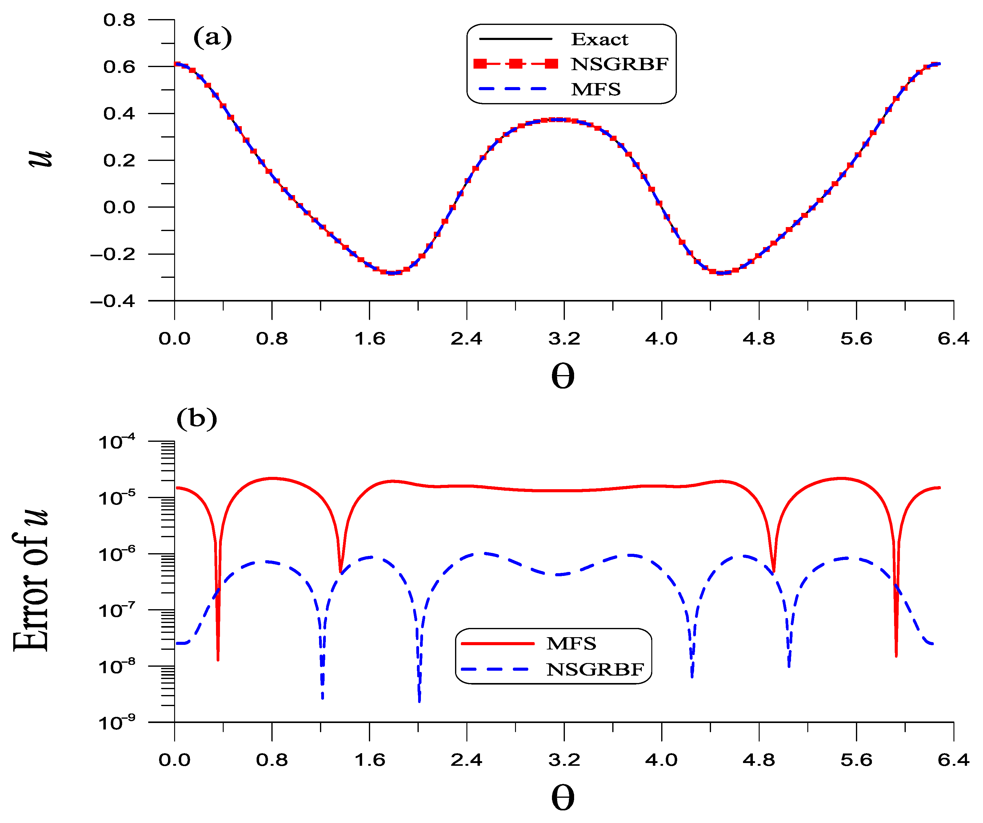
On the curve $\mathcal{C}=\{r=\rho /2,\varphi =\pi /4,0\le \theta \le 2\pi \}$, the numerical solution obtained by MFS is compared to the exact one in Figure 1a, whose error is shown in Figure 1b with ME = $2.18\times {10}^{-5}$.

Figure 1. For example 1 (a) comparing numerical solutions obtained by MFS and NSGRBF with exact one and (b) numerical errors.

By using Equation (63) under $n=1250$, $n_q=1600$, $R_0=0.01$, and $D=7$, we compare the results using different $\beta$ in the NSGRBF in Table 3. For $\beta =0.0001$ the improvement of accuracy comparing to MFS is about three orders. The accuracy is competitive to that computed in [26], which used the method of anisotropic fundamental solution (MAFS) with an optimal value of D; ME = $6.91\times {10}^{-8}$ and RMSE = $3.08\times {10}^{-8}$ were obtained.

Table 3. Solving example 1 by Equation (63); ME and RMSE using different $\beta$.

$\mathit{\beta }$	0.0001	0.8	1.0	1.5	1.95	1.999
ME	$6.91\times {10}^{-8}$	$5.11\times {10}^{-5}$	$5.70\times {10}^{-5}$	$8.02\times {10}^{-5}$	$3.56\times {10}^{-5}$	$1.03\times {10}^{-6}$
RMSE	$2.99\times {10}^{-8}$	$2.48\times {10}^{-5}$	$5.70\times {10}^{-5}$	$3.76\times {10}^{-5}$	$2.07\times {10}^{-5}$	$6.76\times {10}^{-7}$

When the parameter $\beta$ is near to −1, say $\beta =-0.999$, NSGRBF would lead to worse results of ME = $2.04\times {10}^{-4}$ and RMSE = $8.66\times {10}^{-5}$; comparing to Cond = $4.66\times {10}^{10}$ obtained for $\beta =0.0001$ it with a large condition number Cond = $4.15\times {10}^{13}$ presents the ill-posedness of the linear system.

On the curve $\mathcal{C}$, the numerical solution obtained by NSGRBF with $\beta =0.0001$ is compared to the exact one in Figure 1a, whose error is shown in Figure 1b with ME = $3.81\times {10}^{-8}$, which is much accurate than that obtained by MFS. We have computed the condition number for NSGRBF, which is Cond = $4.66\times {10}^{10}$. For MFS we have Cond = $2.75\times {10}^{11}$, which is larger than that of NSGRBF, even $n=100$ is much smaller than $n=1250$ used in NSGRBF. In MFS if we take a near value of $n=1225$, the condition number increases to Cond = $6.02\times {10}^{16}$, which is much large than Cond = $4.66\times {10}^{10}$; ME = $6.63\times {10}^{-8}$ obtained by MFS is still larger than ME = $3.81\times {10}^{-8}$ obtained by NSGRBF. So one major advantage of the NSGRBF is that the resulting linear system is less ill-conditioned that that of MFS and the accuracy of NSGRBF is better than MFS.

To observe the convergence behavior of NSGRBF, we take a different value of m in Equation (63) and list ME and RMSE in Table 4, where $n_q=1600$, $R_0=0.01$, $D=7$, and $\beta =0.0001$ were fixed. It can be seen that the solution is convergent very fast when m increases from 25 to 400.

Table 4. Solving example 1 by Equation (63); ME and RMSE using different m.

m	25	64	100	144	225	400	625
ME	$2.61\times {10}^{-1}$	$8.18\times {10}^{-4}$	$1.09\times {10}^{-5}$	$1.67\times {10}^{-6}$	$8.48\times {10}^{-8}$	$6.85\times {10}^{-8}$	$6.91\times {10}^{-8}$
RMSE	$1.18\times {10}^{-1}$	$2.65\times {10}^{-4}$	$3.38\times {10}^{-6}$	$5.44\times {10}^{-7}$	$4.72\times {10}^{-8}$	$2.80\times {10}^{-8}$	$2.99\times {10}^{-8}$

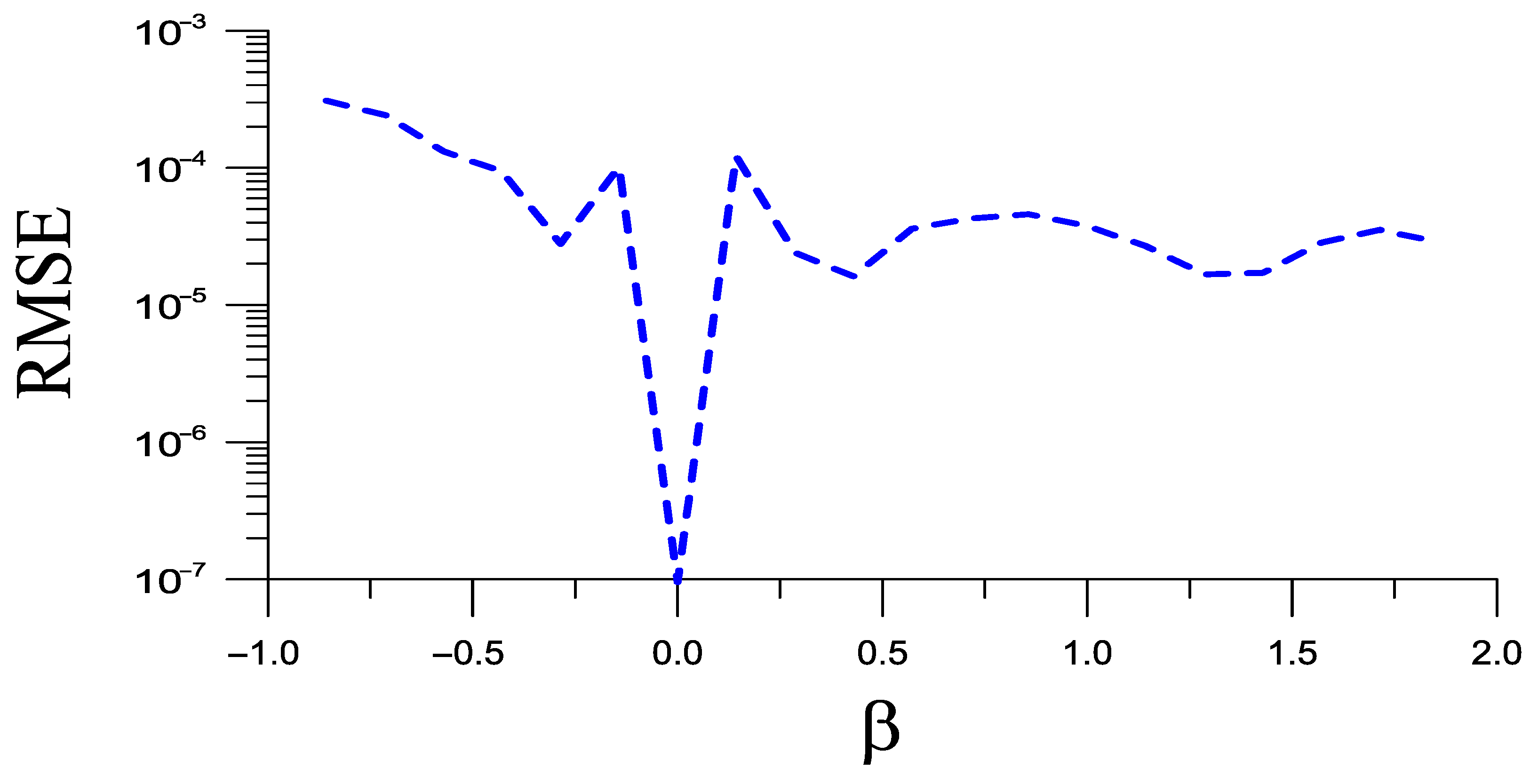
To test the sensitivity of NSGRBF with respect to $\beta$, the RMSE is plotted in Figure 2, where we can observe that when $\beta$ nears zero the best value of RMSE can be obtained. With $\beta <0$ the basis is singular, which is, in principle, less accurate than that with the non-singular basis with $\beta >0$.

Figure 2. For example 1 showing the sensitivity of RMSE obtained by NSGRBF with respect to $\beta$.

5.2. Example 2

In this and next examples, we consider the anisotropic Laplace equation:

$$\begin{array}{c}{k}_{11}{u}_{xx}(x,y,z)+k_{22}{u}_{yy}(x,y,z)+k_{33}{u}_{zz}(x,y,z)\hfill \\ +2k_{12}{u}_{xy}(x,y,z)+2k_{13}{u}_{xz}(x,y,z)+2k_{23}{u}_{yz}(x,y,z)=0,(x,y,z)\in \mathrm{\Omega }\subset {\mathbb{R}}^3,\hfill \end{array}$$

(69)

where the coefficients are subjected to the following constraints [22]:

$$k_{11}>0,k_{22}>0,k_{33}>0,k_{11}{k}_{22}-k_{12}^2>0,k_{11}{k}_{33}-k_{13}^2>0,k_{22}{k}_{33}-k_{23}^2>0.$$

(70)

The numerical solutions of the anisotropic Laplace equation can be carried out by using the proposed NSGRBF or WSMFS depending on the value of the parameter $\beta$.

As an example we take $k_{11}=1$, $k_{22}=1$, $k_{33}=1/2$ and $k_{23}=-1/2$, and the exact solution is given by

$$u(x,y,z)=x^2-y^2-2yz-2z^2.$$

(71)

We can derive

$${\mathbf{K}}^{-1}=\left[\begin{array}{ccc}1& 0& 0\\ 0& 2& 2\\ 0& 2& 4\end{array}\right].$$

(72)

We can apply the original MFS with

$$u\left(\mathbf{x}\right)=\sum _{j=1}^m{\displaystyle \frac{e_j}{\sqrt{{\mathbf{r}}_j^T\left(\mathbf{x}\right){\mathbf{K}}^{-1}{\mathbf{r}}_j\left(\mathbf{x}\right)}}},$$

(73)

to solve Equation (69). Under $n=m^2=625$, $n_q=1600$, $R_0=0.01$, and with the optimal value of $D=9.45$, we obtain ME = $1.58\times {10}^{-5}$ and RMSE = $2.41\times {10}^{-6}$. They are used as referenced values to evaluate the accuracy of the newly proposed methods.

Under $n=1250$, $n_q=1600$, $R_0=0.01$, and $D=7$, we compare the results computed by Equation (64) using different $\beta$ in Table 5. ME and RMSE are given in the whole domain with 12,500 testing points.

Table 5. Solving example 2 by Equation (64); ME and RMSE using different $\beta$.

$\mathit{\beta }$	$-0.0001$	0.0001	0.0005	0.01
ME	$6.79\times {10}^{-6}$	$5.94\times {10}^{-6}$	$7.30\times {10}^{-6}$	$2.64\times {10}^{-5}$
RMSE	$1.29\times {10}^{-6}$	$1.12\times {10}^{-6}$	$2.31\times {10}^{-6}$	$1.94\times {10}^{-5}$

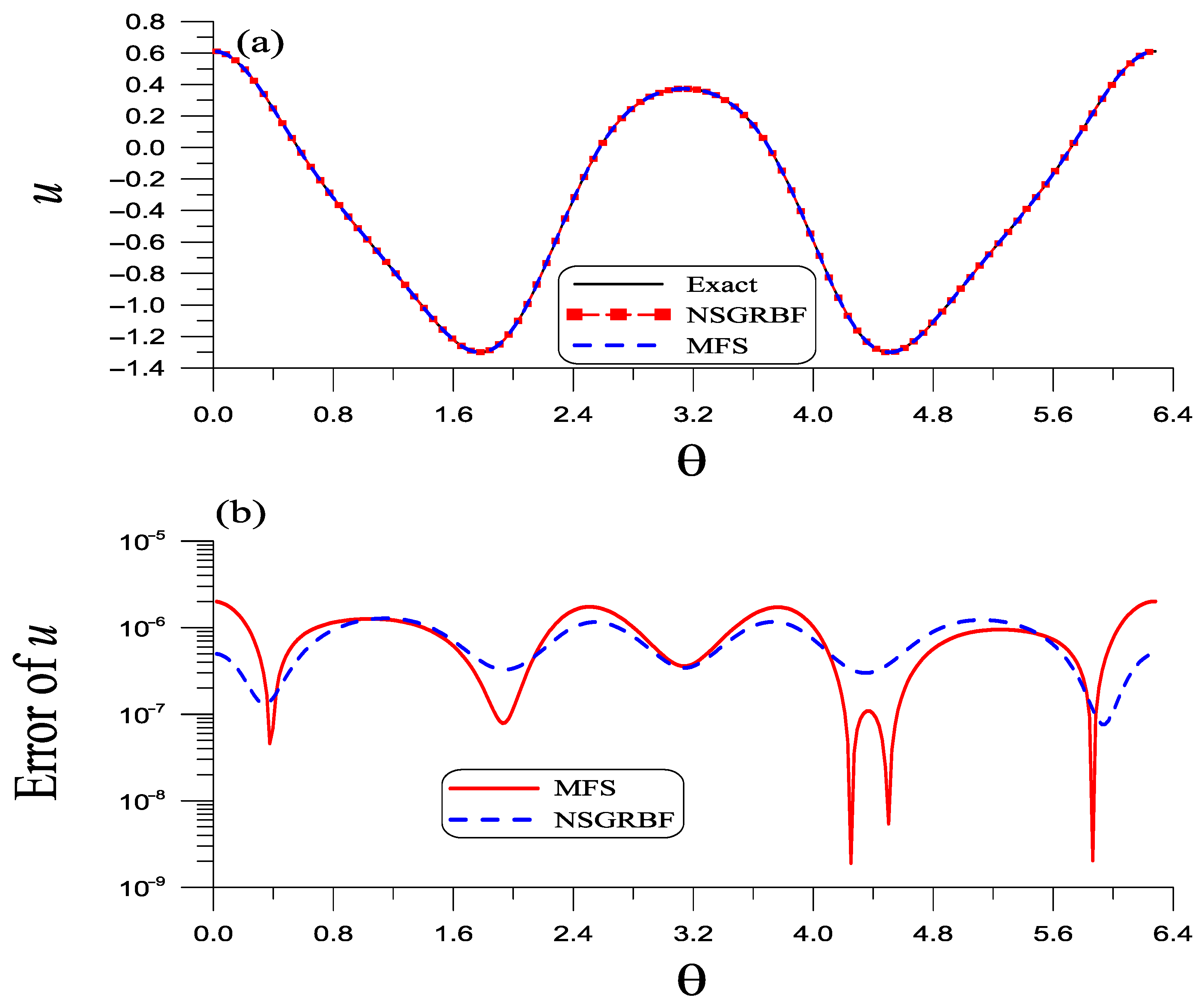
On the curve $\mathcal{C}=\{r=\rho /2,\varphi =\pi /4,0\le \theta \le 2\pi \}$, the numerical solution obtained by MFS is compared to the exact one in Figure 3a, whose error is shown in Figure 3b with ME = $2.01\times {10}^{-6}$.

Figure 3. For example 3 (a) comparing numerical solutions obtained by MFS and NSGRBF with exact one and (b) numerical errors.

On the curve $\mathcal{C}$, the numerical solution obtained by NSGRBF with $\beta =0.0001$ is compared to the exact one in Figure 3a, whose error is shown in Figure 3b with ME = $1.28\times {10}^{-6}$, which is more accurate than that obtained by MFS. The condition number for NSGRBF with $n=1250$ is Cond = $6.60\times {10}^{10}$. For MFS we have Cond = $2.06\times {10}^9$, of which $n=625$ is smaller than $n=1250$ used in NSGRBF. One major advantage of the NSGRBF is that the resulting linear system is less ill-conditioned that that of MFS and the accuracy of NSGRBF is better than MFS.

To observe the convergence behavior of NSGRBF, we take different values of m in Equation (64) and list ME and RMSE in Table 6, where $n_q=1600$, $R_0=0.01$, $D=7$, and $\beta =0.0001$ were fixed. It can be seen that the solution is convergent very fast when m increases from 25 to 400.

Table 6. Solving example 1 by Equation (64); ME and RMSE using different m.

m	25	64	144	225	400	625
ME	$7.64\times {10}^{-2}$	$2.90\times {10}^{-4}$	$5.01\times {10}^{-5}$	$2.42\times {10}^{-5}$	$7.94\times {10}^{-6}$	$5.94\times {10}^{-6}$
RMSE	$5.65\times {10}^{-2}$	$1.33\times {10}^{-4}$	$5.56\times {10}^{-6}$	$2.85\times {10}^{-6}$	$1.57\times {10}^{-6}$	$1.12\times {10}^{-6}$

The logarithmic MFS (LMFS) is also used to solve the anisotropic Laplace equation. Under $n=625$, $n_q=1600$, $R_0=0.01$, and $D=15$, ME = $1.35\times {10}^{-3}$ and RMSE = $5.28\times {10}^{-4}$ are obtained by LMFS.

To enhance the accuracy the LMFS revealed in Equation (65) is employed to solve this problem. Under $n=1250$, $n_q=1600$, $R_0=0.01$, we compare the results computed by Equation (65) using different D in Table 7. ME and RMSE are given in the whole domain with 12,500 testing points. Comparing to Table 5, LMFS is less accurate than the results obtained by NSGRBF and WSMFS.

Table 7. Solving example 2 by Equation (65); ME and RMSE using different D.

D	4	6	7	10	15	20
ME	$1.12\times {10}^{-3}$	$1.07\times {10}^{-3}$	$1.19\times {10}^{-3}$	$4.97\times {10}^{-4}$	$2.90\times {10}^{-4}$	$9.19\times {10}^{-4}$
RMSE	$8.47\times {10}^{-4}$	$7.06\times {10}^{-4}$	$7.68\times {10}^{-4}$	$3.79\times {10}^{-4}$	$1.72\times {10}^{-4}$	$4.36\times {10}^{-4}$

5.3. Example 3

Next we consider a more complicated exact solution:

$$u(x,y,z)=x{e}^{x}cos(y+2z)-e^x(y+2z)sin(y+2z),$$

(74)

with the same $k_{11}=1$, $k_{22}=1$, $k_{33}=1/2$ and $k_{23}=-1/2$.

Under $n=1250$, $n_q=1600$, $R_0=0.01$, and $D=7$, we compare the results computed by Equation (64) using different $\beta$ in Table 8. ME and RMSE are given in the whole domain with 12,500 testing points.

Table 8. Solving example 3 by Equation (64); ME and RMSE using different $\beta$.

$\mathit{\beta }$	$-0.99$	$-0.01$	0.0005	0.001	0.01	1.99
ME	1.997	$5.53\times {10}^{-2}$	$7.62\times {10}^{-3}$	$7.52\times {10}^{-3}$	$5.28\times {10}^{-2}$	0.645
RMSE	0.708	$4.06\times {10}^{-2}$	$1.40\times {10}^{-3}$	$1.34\times {10}^{-3}$	$3.87\times {10}^{-2}$	0.478
Cond	$2.13\times {10}^{13}$	$1.49\times {10}^{12}$	$1.32\times {10}^{10}$	$2.56\times {10}^{11}$	$2.53\times {10}^9$	$9.27\times {10}^{18}$

When the parameter $\beta$ is near to −1, say $\beta =-0.99$, it would lead to the failure of NSGRBF as shown in Table 8, where ME = 1.997 and RMSE = 0.708 are incorrect, with a large condition number Cond = $2.13\times {10}^{13}$ to present the ill-posedness of the linear system. Similarly for $\beta =1.99$, ME = 0.645 and RMSE = 0.478 are incorrect, which are with a large condition number Cond = $9.27\times {10}^{18}$ to show that the linear system is highly ill-posed.

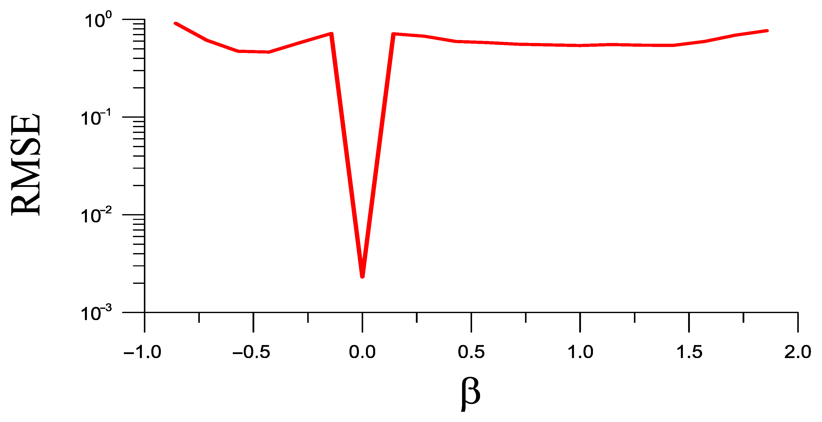
To test the sensitivity of NSGRBF with respect to $\beta$, the RMSE is plotted in Figure 4, where we can observe that when $\beta$ nears to zero the best value of RMSE can be obtained.

Figure 4. For example 3 showing the sensitivity of RMSE obtained by NSGRBF with respect to $\beta$.

Under $n=1250$, $n_q=1600$, $R_0=0.01$, we compare the results computed by Equation (64) using different D and the optimal $\beta$ in Table 9. ME and RMSE are given in the whole domain with 12,500 testing points.

Table 9. Solving example 3 by Equation (64); ME and RMSE using different D.

D	1.5	2	3	4	5	6	7
$\beta$	$6.18\times {10}^{-3}$	$3.82\times {10}^{-3}$	$3.82\times {10}^{-3}$	$6.18\times {10}^{-3}$	$2.36\times {10}^{-3}$	$3.82\times {10}^{-3}$	$6.18\times {10}^{-4}$
ME	$1.33\times {10}^{-4}$	$1.19\times {10}^{-4}$	$1.98\times {10}^{-4}$	$6.65\times {10}^{-4}$	$9.46\times {10}^{-4}$	$4.36\times {10}^{-3}$	$6.70\times {10}^{-3}$
RMSE	$2.64\times {10}^{-5}$	$2.70\times {10}^{-5}$	$1.17\times {10}^{-4}$	$4.91\times {10}^{-4}$	$1.82\times {10}^{-4}$	$2.34\times {10}^{-3}$	$1.15\times {10}^{-3}$

Using $D=2$ and $\beta =3.82\times {10}^{-3}$, ME = $1.19\times {10}^{-4}$ and RMSE = $2.70\times {10}^{-5}$ can be obtained by NSGRBF. Notice that the original MFS in Equation (73) with the optimal value of $D=4.8263$, ME = $7.50\times {10}^{-4}$ and RMSE = $1.39\times {10}^{-4}$ can be obtained, which is less accurate than the present method of NSGRBF.

Rather than the smooth domain in Equations (67) and (68), we consider a unit cube that has eight corners. Let $F=x{e}^{x}cos(y+2z)-e^x(y+2z)sin(y+2z)$ be the exact solution in Equation (74). We impose the following boundary conditions:

$$\begin{array}{c}u(x,y,0)=F(x,y,0),u(x,y,1)=F(x,y,1),\hfill \\ u(0,y,z)=F(0,y,z),u(1,y,z)=F(1,y,z),\hfill \\ u(x,0,z)=F(x,0,z),u(x,1,z)=F(x,1,z).\hfill \end{array}$$

(75)

Under $n=300$, $n_q=600$, $R_0=0.01$, and $D=10$, we compare the results computed by Equation (64) using different $\beta$ in Table 10. ME and RMSE are given in the whole domain with 8000 testing points. It can be seen that ME and RMSE are not sensitive to $\beta$; $\beta =0.5$ leads to a slightly worse value of RMSE.

Table 10. Solving example 3 in a unit cube by Equation (64); ME and RMSE using different $\beta$.

$\mathit{\beta }$	$-0.99$	$-0.05$	0.001	0.5	1.99
ME	$2.16\times {10}^{-2}$	$2.24\times {10}^{-2}$	$2.61\times {10}^{-2}$	$2.82\times {10}^{-2}$	$2.60\times {10}^{-2}$
RMSE	$9.20\times {10}^{-3}$	$5.93\times {10}^{-3}$	$4.56\times {10}^{-3}$	$1.07\times {10}^{-2}$	$6.17\times {10}^{-3}$

6. Conclusions

This paper proposed an order reduction singular MFS to treat the boundary value problems of Laplace equation and anisotropic Laplace equation. The weaker singularity method of fundamental solutions (WSMFS) is endowed with a weaker singularity to raise the accuracy and increase the efficiency due to the reduction of a strong singularity of the original MFS. The non-singular generalized RBF (NSGRBF) solutions were first derived in the literature for both the Laplace equation and anisotropic Laplace equation. The combination of the proposed methods to the traditional MFS can raise the accuracy of the solutions. Numerical experiments assured the efficiency and accuracy of the WSMFS and NSGRBF.

The present paper is equipped with several novelties and significant contributions with a sound mathematical analysis.

1.

We introduced a new idea of singular distance function in terms of a singular projection operator equipped with a parameter $\beta$.

2.

The singular projection operators were derived in closed form for the Laplace equation and anisotropic Laplace equation.

3.

When $2>\beta >0$ the generalized RBF solutions were obtained, which are non-singular.

4.

When $-1<\beta <0$ the generalized RBF solutions were obtained, which are singular with the order of singularity being $-\beta$.

5.

The non-singular generalized RBF (NSGRBF) solutions were derived for the Laplace equation and anisotropic Laplace equation.

6.

The solutions of weaker singularity MFS (WSMFS) were derived for the Laplace equation and anisotropic Laplace equation.

In the future we may extend the present approach of the NSGRBF to other type linear PDEs. For instance $U=cos\lambda r/r$ is the fundamental solution of the 3D Helmholtz equation $\Delta u+{\lambda }^{2}u=0$. We may modify the part $1/r$ by the non-singular solution $r_s^{\beta }$. However, there is still much room to carry out these studies in the future.

References

1. Kupradze, V.D. Potential methods in elasticity. In Progress in Solid Mechanics Volume III; North-Holland Publishing Company: Amsterdam, The Netherlands, 1963; pp. 1–259. [Google Scholar]
2. Prem, K.K. Fundamental Solutions for Differential Operators and Applications; Birkhauser Boston Inc.: Cambridge, MA, USA, 1996. [Google Scholar]
3. Chen, W.; Fu, Z.J.; Chen, C.S. Recent Advances in Radial Basis Function Collocation Methods; Springer: Berlin/Heidelberg, Germany, 2014. [Google Scholar]
4. Fairweather, G.; Karageorghis, A. The method of fundamental solutions for elliptic boundary value problems. Adv. Comput. Math. 1998, 9, 69–95. [Google Scholar] [CrossRef]
5. Cheng, A.H.D.; Hong, Y. An overview of the method of fundamental solutions–solvability, uniqueness, convergence, and stability. Eng. Anal. Bound. Elem. 2020, 120, 118–152. [Google Scholar] [CrossRef]
6. Liu, C.S. An equilibrated method of fundamental solutions to choose the best source points for the Laplace equation. Eng. Anal. Bound. Elem. 2012, 36, 1235–1245. [Google Scholar] [CrossRef]
7. Wang, F.; Liu, C.S.; Qu, W. Optimal sources in the MFS by minimizing a new merit function: Energy gap functional. Appl. Math. Lett. 2018, 86, 229–235. [Google Scholar] [CrossRef]
8. Chen, C.S.; Noorizadegan, A.; Young, D.L.; Chen, C.S. On the determination of locating the source points of the MFS using effective condition number. J. Comput. Appl. Math. 2023, 423, 114955. [Google Scholar] [CrossRef]
9. Wang, F.; Li, X.; Liu, H.; Qiu, L.; Yue, X. An adaptive method of fundamental solutions using physics-informed neural networks. Eng. Anal. Bound. Elem. 2025, 178, 106295. [Google Scholar] [CrossRef]
10. Golberg, M.A.; Chen, C.S. The method of fundamental solutions for potential, Helmholtz and diffusion problems, in Boundary integral methods: Numerical and mathematical aspects. In Comput. Eng., Volume 1. Computer Engineering; WIT Press/Computational Mechanics Publications: Boston, MA, USA, 1999; pp. 103–176. [Google Scholar]
11. Chen, W.; Shen, Z.J.; Shen, L.J.; Yuan, G.W. General solutions and fundamental solutions of varied orders to the vibrational thin, the Berger, and the Winkler plates. Eng. Anal. Bound. Elem. 2005, 29, 699–702. [Google Scholar] [CrossRef]
12. Chen, W. Meshfree boundary particle method applied to Helmholtz problems. Eng. Anal. Bound. Elem. 2002, 26, 577–581. [Google Scholar] [CrossRef]
13. Chen, W.; Tanaka, M. A meshless, integration-free, and boundary-only RBF technique. Comput. Math. Appl. 2002, 43, 379–391. [Google Scholar] [CrossRef]
14. Chen, W.; Shen, Z.J.; Shen, L.J.; Yuan, G.W. Boundary knot method for Poisson equations. Eng. Anal. Bound. Elem. 2005, 29, 756–760. [Google Scholar] [CrossRef]
15. Wang, R.; Wang, F.; Li, X.; Qiu, L. Boundary knot neural networks for the inverse Cauchy problem of the Helmholtz equation. Mathematics 2025, 13, 3029. [Google Scholar] [CrossRef]
16. Liu, L.; Zhang, L.L.; Lei, M.; Niu, R.P. The improved boundary knot method with fictitious points for solving high-order Helmholtz-type PDEs. Comput. Math. Appl. 2005, 191, 36–47. [Google Scholar] [CrossRef]
17. Dehghan, M.; Mohammadi, V. The boundary knot method for the solution of two-dimensional advection reaction-diffusion and Brusselator equations. Int. J. Numer. Meth. Heat Fluid Flow 2021, 31, 106–133. [Google Scholar] [CrossRef]
18. Hon, Y.; Chen, W. Boundary knot method for 2D and 3D Helmholtz and convection–diffusion problems under complicated geometry. Int. J. Numer. Meth. Eng. 2003, 56, 1931–1948. [Google Scholar] [CrossRef]
19. Jin, B.; Zheng, Y. Boundary knot method for some inverse problems associated with the Helmholtz equation. Int. J. Numer. Meth. Eng. 2005, 62, 1636–1651. [Google Scholar] [CrossRef]
20. Lei, M.; Liu, L.; Chen, C.; Zhao, W. The enhanced boundary knot method with fictitious sources for solving Helmholtz-type equations. Int. J. Comput. Math. 2023, 100, 1500–1511. [Google Scholar] [CrossRef]
21. Liu, L.; Lei, M.; Yue, J.H.; Niu, R.P. Modified boundary knot method for multi-dimensional harmonic-type equations. Int. J. Comput. Meth. 2024, 21, 2341004. [Google Scholar] [CrossRef]
22. Shiah, Y.C.; Tan, C.L. BEM treatment of three-dimensional anisotropic field problems by direct domain mapping. Eng. Anal. Bound. Elem. 2004, 28, 43–52. [Google Scholar] [CrossRef]
23. Jin, B.T.; Chen, W. Boundary knot method based on geodesic distance for anisotropic problems. J. Comput. Phys. 2006, 215, 614–629. [Google Scholar] [CrossRef]
24. Rao, N.; Farid, M.; Jha, N.K. A study of (σ, μ)-Stancu-Schurer as a new generalization and approximations. J. Inequal. Appl. 2025, 2025, 104. [Google Scholar] [CrossRef]
25. Ayman-Mursaleen, M. Controllability of Tempered Caputo fractional dynamical systems. J. Nonl. Conv. Anal. 2025, 26, 2501–2511. [Google Scholar]
26. Liu, C.S.; Kuo, C.L. Pseudo and anisotropic MFS for Laplace equation and optimal sources using maximal projection method with a substitution function. Eng. Anal. Bound. Elem. 2024, 158, 313–320. [Google Scholar] [CrossRef]
27. McOwen, R.C. Partial Differential Equations: Methods and Applications, 2nd ed.; Pearson Education Inc.: St. Hoboken, NJ, USA, 2003. [Google Scholar]