Article

Implementing the Linear Adaptive False Discovery Rate Procedure for Spatiotemporal Trend Testing

by
Oliver Gutiérrez-Hernández
1,* and
Luis V. García
2
1
Department of Geography, University of Málaga (UMA), 29071 Málaga, Spain
2
Institute of Natural Resources and Agrobiology of Seville (IRNAS), Spanish National Research Council (CSIC), 41012 Seville, Spain
*
Author to whom correspondence should be addressed.
Mathematics 2025, 13(22), 3630; https://doi.org/10.3390/math13223630
Submission received: 2 October 2025 / Revised: 6 November 2025 / Accepted: 11 November 2025 / Published: 12 November 2025
(This article belongs to the Special Issue Advanced Mathematical Methods in Remote Sensing)

Abstract

Statistical inference in spatiotemporal trend analysis often involves testing separate hypotheses for each pixel in datasets containing thousands of observations. A pixel is considered significant if its p-value falls below a rejection threshold (α). However, this uncorrected approach ignores the large number of simultaneous tests and greatly increases the risk of false positives. This issue, known as multiple testing or multiplicity, can be addressed by controlling the false discovery rate (FDR), defined as the expected proportion of false positives (i.e., false discoveries) among all rejected hypotheses, at a pre-specified control level q. This study implements the linear adaptive two-stage Benjamini–Krieger–Yekutieli (BKY) procedure for FDR control in spatiotemporal trend testing and compares it with two alternatives: the uncorrected significance approach and the original non-adaptive Benjamini–Hochberg (BH) procedure. The BKY method empirically estimates the number of true null hypotheses (m0) and adaptively relaxes the rejection threshold when many true alternatives are present, thereby increasing statistical power without compromising FDR control. Results indicate that the BKY procedure is a recommended approach for large-scale trend testing using spatiotemporal environmental data, particularly in gridded-data-intensive fields such as environmental remote sensing, climatology, and hydrology. To foster reproducibility, R code is provided to apply the BKY procedure and compare it with the uncorrected raw p-values and the BH approach on any gridded dataset.
MSC:
62G10 Hypothesis testing; 62P12 Applications to environmental sciences

1. Introduction

Consider a trend test applied to a single time series of environmental data—such as temperature, precipitation, or a vegetation index—at a significance level of α = 0.05. In this case, if the null hypothesis is true, there is a 5% probability of committing a Type I error, that is, rejecting it incorrectly. The picture dramatically changes with spatially gridded data, where each pixel is subjected to a separate trend test. In this context, thousands of tests are routinely performed, so even if the Type I error rate remains at 5% per test, the absolute number of false positives becomes large, resulting in trend maps where random noise may generate spurious patterns that appear across many pixels rather than genuine environmental signals [1].
Faced with this situation, three different alternatives can be considered: ignoring the problem, trying to eliminate it entirely, or addressing it in a more flexible way. The first alternative corresponds to those who fail to recognise the issue and fall into selective inference [2]; that is, they report only those trends that appear “significant” at a fixed threshold (α, typically 0.05) without considering the complete set of tests performed. In spatio-temporal datasets, this implies conducting thousands of independent contrasts—one for each pixel—which leads to multiplicity problems and a substantial increase in the number of false positives if all p-values are not correctly adjusted [3]. The second alternative is represented by methods that control the family-wise error rate (FWER), which aim to ensure that the probability of committing at least one Type I error across all tests remains below α. While formally correct, such procedures are so conservative in remote-sensing contexts that they drastically reduce statistical power [4], making the detection of genuine signals practically unfeasible. The third alternative suggests a less stringent yet more balanced control strategy—one that accepts the occurrence of some false positives, provided they represent only a limited proportion of the significant results on average. This approach corresponds to the concept of the false discovery rate (FDR) [5].
The FDR concept, introduced by Benjamini and Hochberg [6], is defined as the expected proportion of false discoveries (i.e., incorrectly rejected hypotheses) among all discoveries (i.e., all rejected hypotheses). Thirty years after its introduction in 1995, the FDR has become the standard approach for multiple testing correction across many scientific disciplines, ranking among the most highly cited statistical contributions in modern science [7,8]. However, it has rarely been applied in remote sensing [9,10,11,12,13], most likely due to a combination of methodological inertia and limited statistical training within the field, which has exposed a serious problem for the reliability of large-scale inference in environmental remote sensing, climatology and hydrology [14].
In this study, this gap is addressed by adopting the adaptive FDR procedure proposed by Benjamini, Krieger, and Yekutieli (2006) (BKY) [15], while the original approach of Benjamini and Hochberg (1995) (BH) [6] is also considered for comparison. The original BH approach assumes that all null hypotheses are true. In contrast, the adaptive version increases statistical power by estimating the proportion of true null hypotheses within the set of tests, making it particularly well-suited for gridded environmental datasets. This study aims (i) to highlight the need for implementing FDR control in spatially gridded trend detection, and (ii) to present evidence supporting the recommendation of the adaptive BKY procedure, accompanied by reproducible R code that facilitates its application in environmental research.

2. Methods

2.1. Foundations of FDR

A multiple testing problem arises when a large number of hypotheses are evaluated simultaneously [16]. According to Farcomeni (2006) [17], Table 1 summarises the possible outcomes of multiple testing, distinguishing between correct decisions and the two types of statistical errors.
In single-test situations, the objective is to control the probability of a false rejection. However, when thousands of tests are conducted simultaneously—as in spatio-temporal trend tests—the risk of false positives increases. Consequently, the focus shifts from individual tests to the collective behaviour of all hypotheses, aiming to control the overall proportion of false discoveries. From a practical perspective, the challenge lies in minimising false negatives without allowing an excess of false positives.
The FDR was defined in Benjamini & Hochberg (1995) [6] as the expected proportion of false discoveries among all discoveries (Equation (1)):
FDR = E V R
where
E denotes the expected value.
V is the number of false positives (false discoveries).
R is the total number of rejected hypotheses (discoveries).
The FDR approach aims to keep this proportion below a predefined control level q, typically controlled at q = 0.05 [6], within the subset of p-values that were found to be statistically significant under the FDR criterion (i.e., tests with p-values below an FDR-defined critical p-value), after performing multiple (m) hypothesis tests at the pixel-scale. In other words, the FDR control guarantees that (Equation (2)):
FDR = E V R q

2.2. Procedures for FDR Control

Over the past three decades, a wide range of methods has been proposed, among which step-up procedures—based on sequentially increasing rejection thresholds—have become particularly prominent [5]. The following section focuses on two widely adopted variants, culminating in an adaptive approach, which has proven particularly relevant for large, spatially gridded datasets.

2.2.1. The Benjamini–Hochberg Procedure (BH)

Benjamini and Hochberg (1995) [6] began by considering the simultaneous testing of multiple null hypotheses H1, H2, , Hm based on their corresponding p-values p1, p2, , pm, where H(i) denotes the null hypothesis associated with the ordered p-value p(i). The Benjamini–Hochberg (BH) procedure can be regarded as a Bonferroni-type approach, as it defines significance thresholds as a function of the total number of hypotheses tested [18]. Unlike the Bonferroni correction, which limits the probability of making any false rejection (family–wise error rate, FWER), the BH procedure controls the expected proportion of false discoveries (FDR), aiming to increase statistical power to detect true effects while maintaining rigorous control of false discoveries—a particularly valuable property in large-scale inference common in environmental remote sensing, climatology and hydrology [19].
The BH procedure assumes that individual tests are either independent or positively dependent [5,6,20]. Although it does not require all null hypotheses to be true, it determines rejection thresholds as if all null hypotheses were null. In doing so, it uses the total number of hypotheses m , rather than estimating the number of true nulls m 0 . This conservative design ensures strict FDR control even under the global null ( m 0 = m ), where all hypotheses are true. Under these conditions, the expected proportion of false discoveries remains at or below the pre-specified level, typically q = 0.05 , which plays a role analogous to the significance level α in individual hypothesis testing.
To apply the procedure, the researcher first sets a desired FDR level q . The Benjamini–Hochberg (BH) algorithm is then implemented as follows:
  • Step 1. Order the p-values of all the hypothesis tests in ascending order (Equation (3)):
p ( 1 ) p ( 2 ) p ( m )
where
p 1 represents the smallest p-value; p 2 the second smallest p-value; p m  the largest p-value; and m is the total number of hypothesis tests performed.
  • Step 2. Identify k as the largest value of i such that (Equation (4)):
p i i m q
where
p i denotes the p-value with rank i, in ascending order among the m hypothesis tests; i is the rank of the p-value when ordered from smallest to largest; m is the total number of hypothesis tests performed; q is the desired FDR level. The corresponding p-value at position k  ( p k = k m q )  is referred to as the critical p-value, which defines the rejection threshold for the BH procedure.
  • Step 3. The final step is to reject all null hypotheses corresponding to p-values up to position k (Equation (5)):
H 1 , H 2 , , H k
where
H 1 denotes the hypotheses corresponding to the smallest p-value; H 2 the second smallest p-value; H k , to the hypothesis associated with p ( k ) , which is the highest-ranked hypothesis that satisfies the BH criterion.

2.2.2. The Benjamini-Krieger-Yekutieli Procedure (BKY)

The adaptive procedure proposed by Benjamini, Krieger, and Yekutieli (2006) [15] extends the original single-stage BH procedure into a two-stage framework. Its key idea is that the value of m 0 —the number of true null hypotheses—can be estimated from the results of the BH procedure itself. Rather than computing rejection thresholds under the conservative assumption that m 0 = m , the BKY procedure estimates m 0 from the data and adjusts the rejection threshold accordingly. When m 0 < m —that is, when some hypotheses are truly non-null—the procedure relaxes the rejection criterion, thereby increasing statistical power while still controlling the FDR under independence and positive dependence. This makes the method particularly advantageous in settings where the proportion of true alternatives (non-null hypotheses) is high, offering a more adaptive and less stringent alternative to the original BH approach.
As in the BH procedure, a predefined FDR level q (typically 0.05) is first set by the researcher. The Benjamini–Krieger–Yekutieli (BKY) procedure is then applied as follows:
  • Step 1. Apply the linear step-up BH procedure at a reduced significance level q′, defined as (Equation (6)):
q = q 1 + q
Count how many hypotheses are rejected; denote this number as r 1 .
  • If r 1 = 0 : no hypothesis is rejected, and the procedure stops.
  • If r 1 = m : all hypotheses are rejected, and the procedure stops.
  • Otherwise, proceed to Step 2.
This initial set of rejections ( r 1 ) provides a preliminary indication of how many hypotheses are likely to be non-null.
  • Step 2. Use the complement to r 1 to obtain a conservative estimate of the number of true null hypotheses ( m ^ 0 ), as shown in (Equation (7)):
m ^ 0 = m r 1
where
m is the total number of hypotheses tested; and, r 1  is the number of hypotheses rejected in Step 1.
  • Step 3. Apply the linear step-up BH procedure again, using the adjusted significance level q (Equation (8)):
q = q m m 0 ^
where
q is the reduced FDR level from Step 1; m is the total number of hypotheses; and m ^ 0  is the estimated number of true null hypotheses from Step 2.
Reject all hypotheses satisfying, as shown in Equation (9):
p i i m q
where
p i is the i-th ordered p-value; i is the rank of the p-value; m is the total number of hypotheses; m is the total number of hypotheses; q is the adjusted FDR threshold.
This step adaptively relaxes the rejection threshold when evidence suggests that many hypotheses are non-null, thereby increasing statistical power while maintains FDR control.
Therefore, when explicitly stating the estimated proportion of true null hypotheses (m0/m), the FDR is expressed as follows (Equation (10)):
FDR = E V R m 0 m q
Equation (10) shows that when m0m, the original BH procedure tends to be conservative, controlling the FDR at a threshold substantially below the nominal q. Incorporating the empirical estimate of m0 allows for a higher adjusted significance threshold (q) compared to the original BH method, which implicitly assumes m0/m = 1. In practice, the adaptive BKY procedure enables the detection of a greater number of true effects on average than the non-adaptive BH, while still controlling the FDR at the fixed level q.
Note that in practical implementations (see Section 2.4. Software Implementation and Reproducibility), the adaptive procedure is often reported in terms of the estimated proportion of true null hypotheses (π0 = m0/m) rather than the absolute number (m0). Both notations are equivalent, since the two quantities are directly related through the total number of tests m. Figure 1 represents the FDR-BH and FDR-BKY workflow.
In summary, the adaptive FDR–BKY procedure extends the original FDR–BH framework by introducing a data-driven estimation of the number of true null hypotheses. This adaptive step enables a more efficient compromise between discovery and error control, enhancing sensitivity while maintaining rigorous control of the false discovery rate.

2.2.3. Features and Advantages of FDR Control

This section outlines several operational features and practical advantages of procedures designed for FDR control, focusing on aspects that make them particularly suitable for large-scale multiple testing [19].
Firstly, these procedures can be applied rapidly and efficiently, as they only require the computation and ordering of p-values, making them practical even for very large datasets [21]. They can also be combined with any valid statistical test, offering full versatility, and they remain straightforward to implement directly from p-values without requiring additional distributional assumptions [6].
As noted by Benjamini (2010) [5], the FDR is an intuitive criterion that adaptively spans the entire range from extreme multiplicity control to none, depending on the data encountered. In practice, this means that FDR control adjusts dynamically to the characteristics of the data—becoming more permissive when true signals are abundant and more conservative when they are scarce—thus maintaining a sensible balance between discovery and reliability across different analytical scales. Ultimately, it is interpretable from multiple perspectives, ranging from frequentist to Bayesian and decision-theoretic frameworks [22,23,24,25].
FDR control remains stable under dataset expansion, a property that reflects its asymptotic behaviour as the number of hypotheses increases [26]. Additionally, it is flexible regarding the definition of rejection thresholds, which depend on the global distribution of p-values rather than fixed significance levels [27].
Finally, FDR control remains robust under positive dependence among tests [20], a common condition in image-based analyses where neighbouring pixels exhibit spatial autocorrelation. This robustness has also been demonstrated in gridded environmental data [28,29,30], where spatial dependence is intrinsic to the structure of the observations.

2.3. Application: From a Limited Dataset to a Real Case Study

To illustrate the mechanics of FDR control before turning to a real case study, a limited dataset of 100 ordered p-values is first considered. This limited dataset makes the step-up procedure transparent. It highlights the practical differences between the original BH threshold and its adaptive two-stage variant (BKY) at a nominal FDR level of q = 0.05. The p-values are generated with a fixed seed to ensure full reproducibility; the adaptive illustration assumes m0 = 60 for expository purposes. In addition, the stability of the m 0 / m ratio was evaluated through a Monte Carlo simulation (10,000 replications) under the same conditions, providing a quantitative measure of the reliability of this adaptive estimation. The complete R code, along with the limited dataset, is provided in the Supplementary Material.
For the real-world application, the FDR procedures were applied to the results of a Contextual Mann–Kendall (CMK) trend test [31], which accounts for spatial autocorrelation, combined with a prewhitening correction for temporal autocorrelation [32]. The analysis was conducted on the Advanced Very High-Resolution Radiometer (AVHRR) normalised difference vegetation index (NDVI) [33] data from the vegetation health products (VHP) provided by the National Oceanic and Atmospheric Administration’s Center for Satellite Applications and Research (NOAA STAR). The dataset, originally at 4 km resolution, was resampled to 10 min using bilinear interpolation, covering 481,499 pixels globally.
A total of 2184 weekly raster images spanning 42 years (1982–2023) were processed. Missing or corrupted values due to cloud contamination or sensor noise were corrected through linear temporal interpolation, while erroneous pixels were adjusted using harmonic regression [34]. From this curated dataset, an annual spatiotemporal time series representing the median NDVI per year was derived. The use of the median is less sensitive to outliers and extreme values [35]. It ensured a robust indicator of central tendency for long-term vegetation trend analysis. Finally, the 481,499 spatially gridded p-values obtained from the CMK trend tests were adjusted for multiple comparisons using the BH and BKY procedures.
Although it is commonly assumed that spatial datasets exhibit positive dependence [36], this assumption was verified by calculating Moran’s I [37] on the p-value map obtained from the Contextual Mann–Kendall (CMK) trend test for different spatial window sizes. This step ensures that the data meet the assumption of independence or at most moderate positive spatial dependency, essential for practically applying FDR procedures.

2.4. Software Implementation and Reproducibility

Spatial and temporal gridded data processing, as well as the application of spatiotemporal trend tests, were carried out using the Series Trend Analysis module of the Earth Trends Modeller (ETM) within the TerrSet Geospatial Monitoring and Modelling Software (version 20.0.3) [38]. Using this GIS software, the raw p-value map was obtained. This output was then converted to GeoTIFF format with LZW compression, setting −9999 as the no-data value, and adopting the Equal Earth projection (EPSG: 8857), which preserves area equivalence across the globe [39].
For the implementation, the original FDR control following Benjamini–Hochberg (BH) was carried out using the stats package in R (version 4.5.1) [40], which is part of the base distribution. The adaptive Benjamini–Krieger–Yekutieli (BKY) procedure was applied through the cp4p package (version 0.3.6) [41], which in turn depends on the multtest library (version 2.6.4) [42,43]. A custom wrapper was developed to extend these procedures to raster data structures via the terra package (version 1.8.80) [44].
To assess the spatial dependency structure of the p-value map, global Moran’s I was computed using the terra package [44] with normalised Queen’s case neighbourhood matrices of increasing window sizes (3 × 3, 5 × 5, 7 × 7, 9 × 9, and 11 × 11). This multiscale approach allowed evaluating the decay of spatial autocorrelation with spatial support, ensuring consistency with the default implementation of terra while maintaining comparability across neighbourhood configurations [45,46]. All calculations were performed on the same gridded dataset to ensure consistency and comparability across window sizes.
In the Supplementary Material, the complete R code for the implementation is provided. Along with the code, a p-value map illustrating the workflow is also included; this example can be replaced by any raster of p-values with a similar format. This Supplementary Material serves a dual purpose: to ensure the verifiability of the results and to facilitate usability, enabling researchers to readily apply the workflow to their own datasets.

3. Results

3.1. Limited Dataset: Graphical Comparison of p-Value Rejection Thresholds

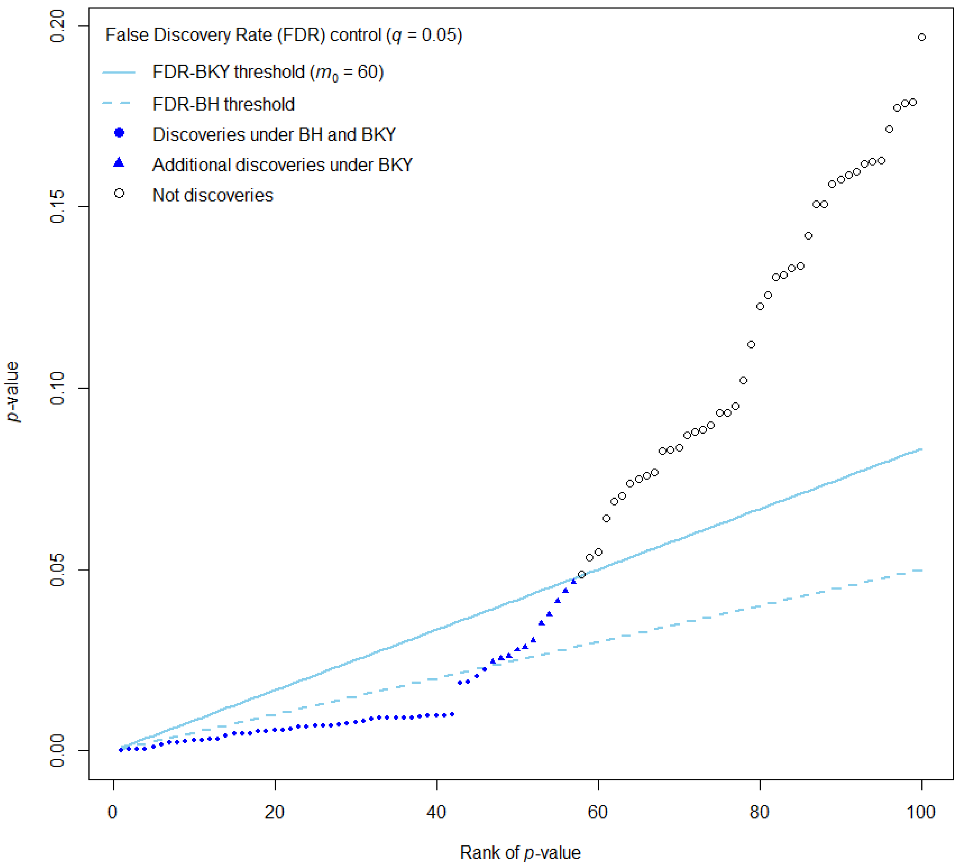
Figure 2 shows the results of the limited dataset with 100 p-values, of which 40 correspond to alternatives and 60 to true null hypotheses ( m 0 = 60 ). At the nominal control level of q = 0.05 , both the BH and the adaptive BKY procedures identified a standard set of significant tests. Still, the adaptive BKY produced additional rejections beyond those obtained with BH.
Below, each graphical element is described in relation to the corresponding equations introduced in Section 2.2.1 and Section 2.2.2. Following Equation (3), p-values are displayed in increasing order as p ( i ) : the x-axis shows the ranks i and the y-axis the ordered values p ( i ) . The dashed line corresponds to Equation (4), representing the BH linear step-up threshold p ( i ) = i m q . The cutoff ( p ( k ) ) see the note alongside Equation (4) that defines the set of rejections, as expressed in Equation (5), is visually indicated by the intersection between the ordered p-values and this threshold, and the corresponding rejected hypotheses are shown as filled diamonds. The solid line represents Equation (8) from the adaptive BKY procedure, where the threshold is redefined as p ( i ) = i m q * using the estimated number of true nulls. In this illustrative example, m 0 = 60 is a known value from the simulated data, but in real applications m 0 is always unknown and must be estimated. The additional rejections obtained under Equations (8) and (9) appear as triangles, while the open circles above both lines correspond to non-rejected hypotheses.
The ratio m 0 / m remained highly stable across 10,000 replications, with a mean estimated value of 0.608 (bias = 0.008, SD = 0.011, RMSE = 0.013) and a 95% empirical interval [0.582, 0.620]. These results confirm that the estimation of m 0 / m is robust under repeated sampling and can reliably support adaptive FDR control.

3.2. Real Case Study: From Raw p-Values to FDR-Adjusted Discoveries

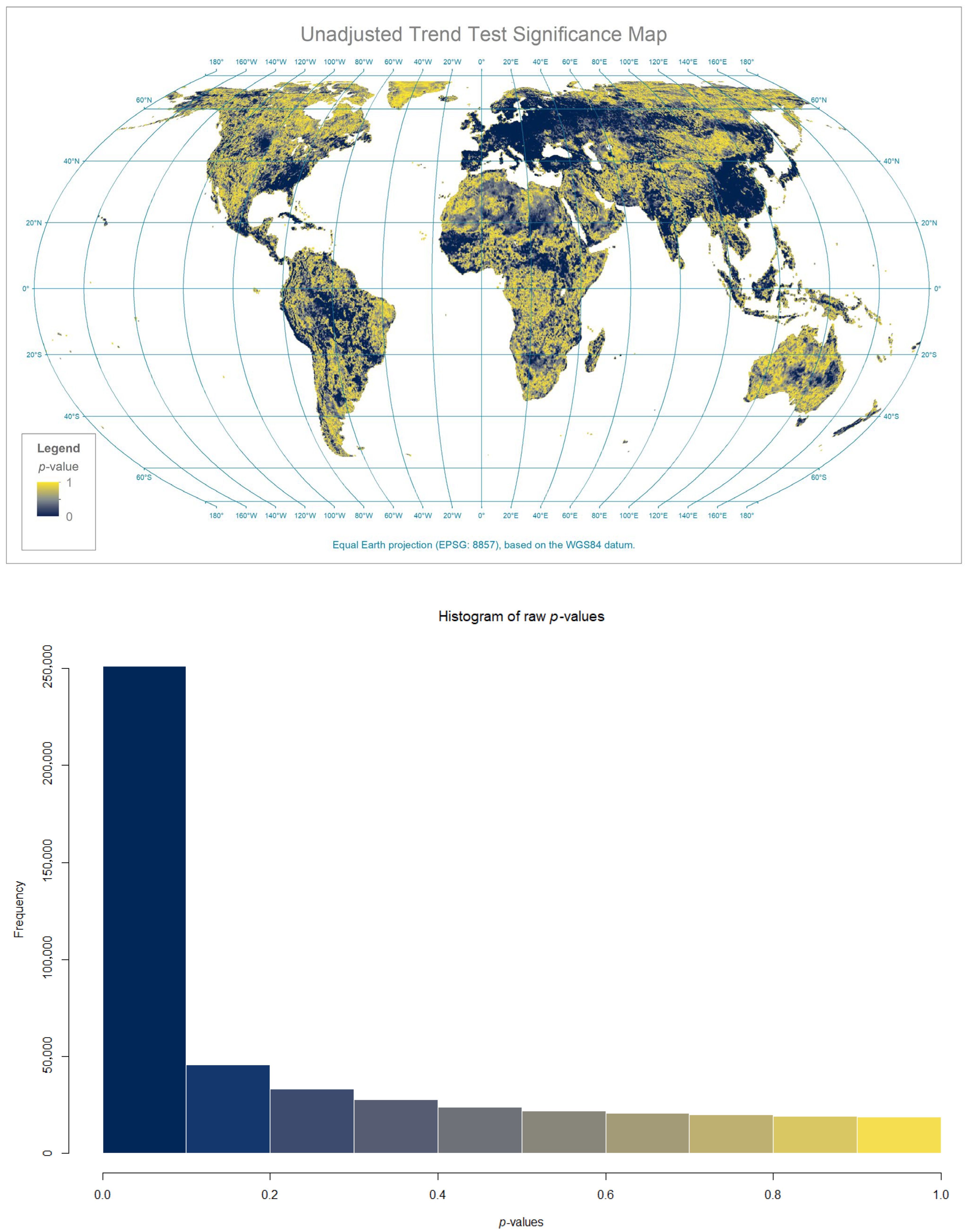
Figure 3 shows the global distribution and frequency of the 481,499 raw p-values obtained from the CMK trend test. Global Moran’s I values were 0.60 (p = 0.55) for the 3 × 3 neighbourhood, 0.49 (p = 0.63) for 5 × 5, 0.41 (p = 0.68) for 7 × 7, 0.37 (p = 0.71) for 9 × 9, and 0.33 (p = 0.74) for 11 × 11 windows, respectively. These results indicate moderate positive spatial autocorrelation that gradually weakens with increasing spatial support, while the associated p-values confirm that the effect is not statistically significant at the global level. These calculations can be fully reproduced with the code and dataset provided in the Supplementary Material.
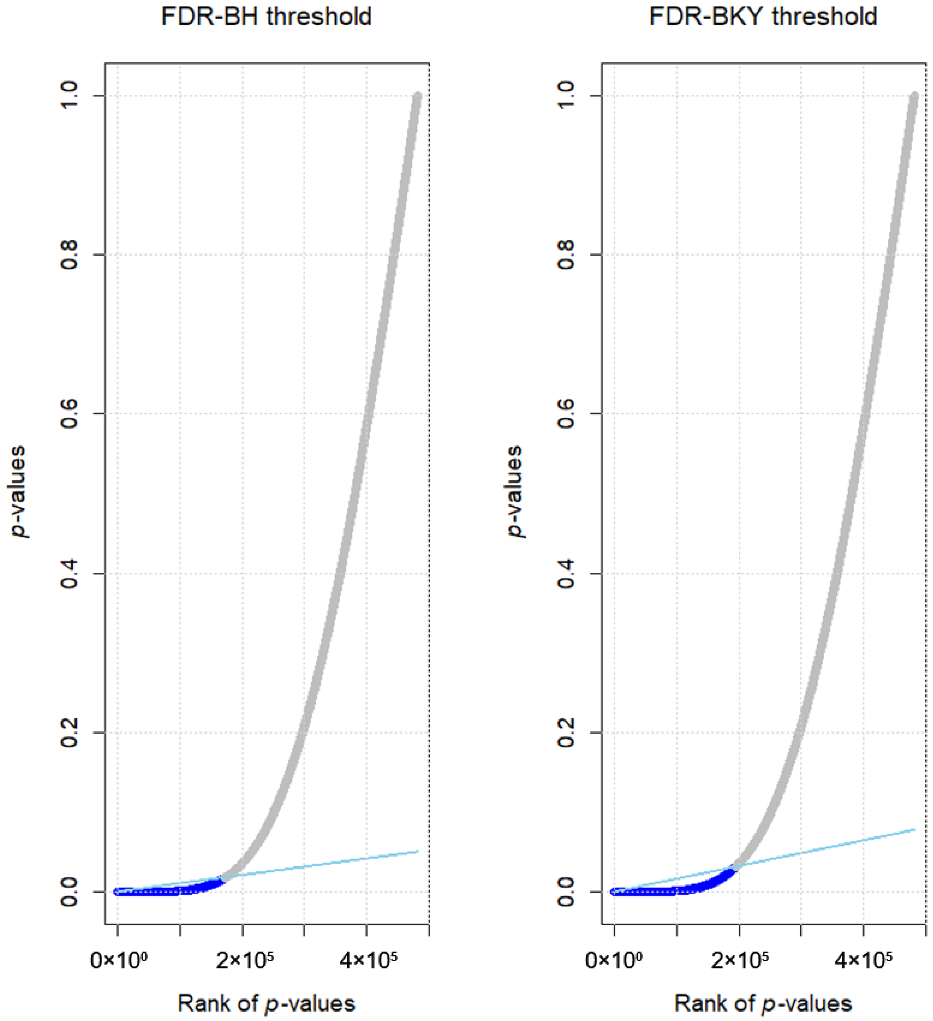
As shown in Figure 4, the adaptive BKY procedure yielded a π0 estimate of 0.6452, producing a higher number of discoveries compared to the classical BH method. The effect of relaxing the rejection threshold is evident in the right panel, where the adaptive threshold line exhibits a slightly steeper slope than the BH threshold on the left.
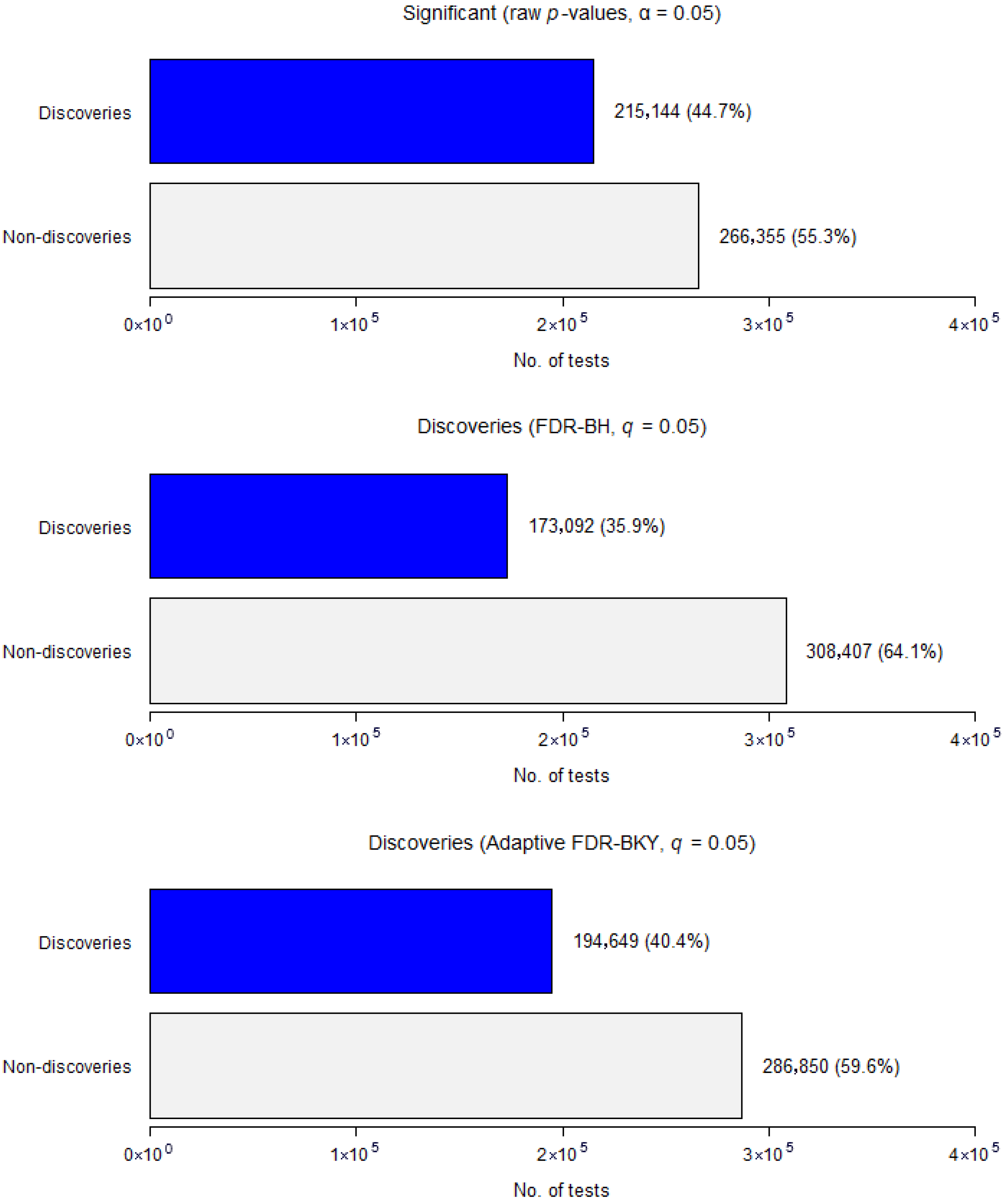
Using a raw significance threshold at α = 0.05, 215,144 pixels (44.7%) appeared significant (Figure 5). However, after applying multiple testing correction, the number of discoveries decreased: the classical BH procedure retained 173,092 significant trends (35.9%), while the adaptive BKY procedure increased the count to 194,649 (40.4%).
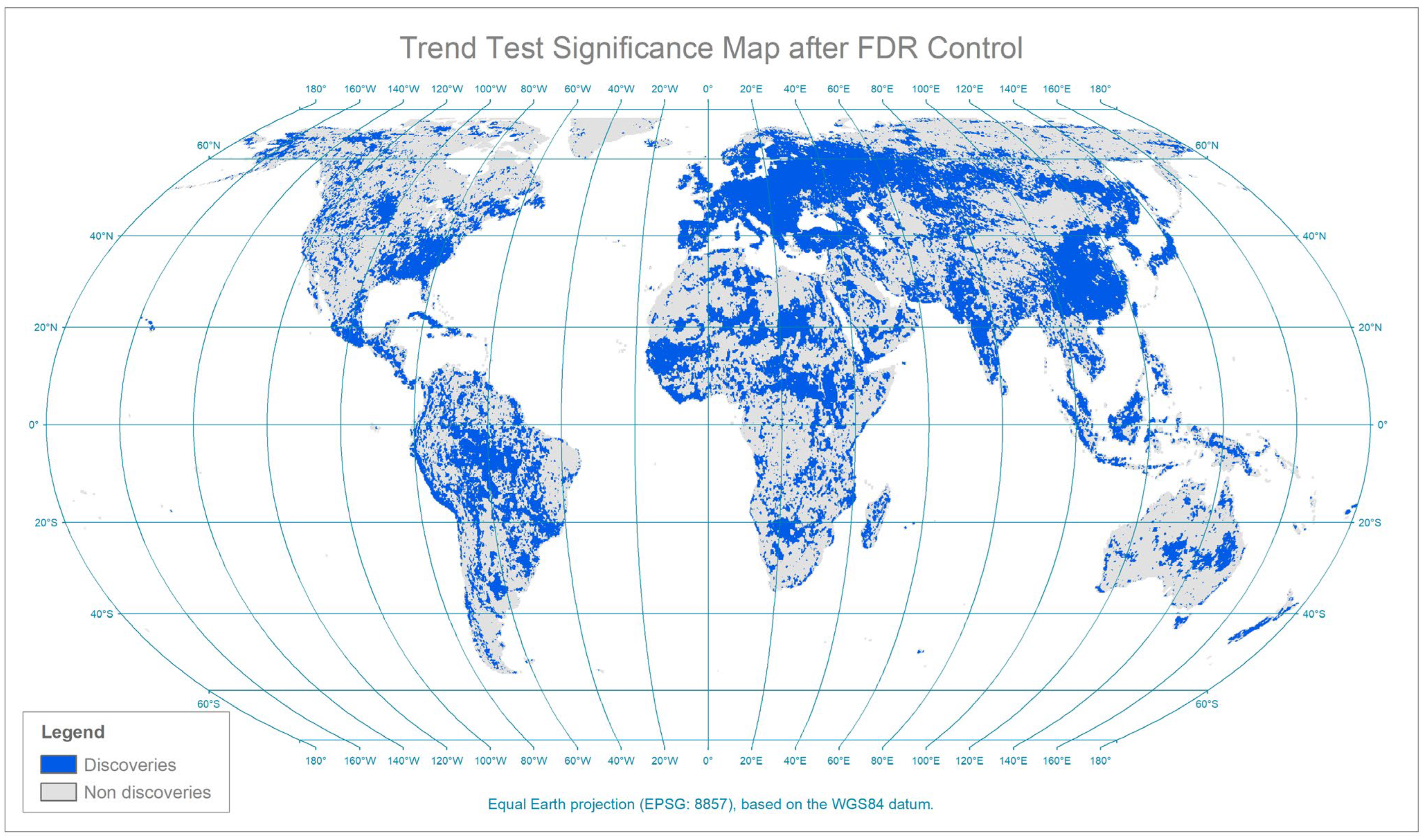
Figure 6 maps the spatial distribution of significant trends after FDR control (q = 0.05). The retained rejections (discoveries) highlight spatially coherent areas where trends are statistically supported. In this context, the binarisation of results is meaningful, as it explicitly accounts for multiple testing and reflects only those locations where the null hypothesis was reliably rejected after FDR control.

4. Discussion

4.1. Interpretation of FDR Control and the Adaptive Approach

This study examines the performance of FDR procedures in controlling false discoveries in spatiotemporal trend testing from gridded data. Using both a limited dataset of 100 p-values and a real-world case study of 481,499 p-values, it was shown that the adaptive BKY procedure identifies more discoveries (significant trends) than the classical BH, while both methods reduce the inflation of apparent significance observed under raw testing.
To better interpret these findings, it is essential to recall the distinction between the original significance level α and the FDR level q. A threshold of α = 0.05 controls the probability of committing a type I error in each test, but does not control the overall proportion of false positives among all declared significant results. In the case study, using an uncorrected threshold of α = 0.05, 245,835 pixels were flagged as significant. However, under this approach, the 5% error rate applies only to individual tests, not to the entire set of declared significant results; consequently, the expected proportion of spurious trends remains uncontrolled. By contrast, an FDR threshold of q = 0.05 controls the expected proportion of false discoveries, ensuring that, on average, no more than 5% of all declared discoveries are false. While some studies refer to an “adjusted α” in the context of multiple testing, it is preferable to use q when FDR control is applied, as this parameter directly represents the expected proportion of false discoveries rather than an adjusted significance level.
It is worth noting, as demonstrated through simulations by Miller et al. (2001) [27], that the effect of FDR procedures cannot be replicated by arbitrarily lowering the significance threshold (for example, from α = 0.05 to α = 0.01). Such a strategy reduces the number of rejections but provides no guarantee regarding the proportion of false positives among them. By contrast, FDR procedures adapt the rejection threshold to the observed distribution of p-values, thereby offering an explicit error-control framework. In this way, FDR does not merely make significance testing more stringent, but redefines it under conditions of multiplicity, turning raw p-values into declared statistically meaningful discoveries. Consequently, lowering α reduces rejections without ensuring the global validity of the results. In contrast, FDR procedures may reduce or recover rejections depending on the proportion of true effects in the data, while maintaining FDR control. Consequently, FDR adjustment does not necessarily entail a reduction in the number of rejected hypotheses; instead, it adapts them to the data while ensuring error control on average. Thus, when FDR reduces the number of rejections, it is because the procedure prevents spurious patterns in the data from being declared significant, thereby safeguarding the validity of the discoveries.
In the adaptive BKY procedure, the FDR control is further refined through an empirical estimation of the number of true null hypotheses (m0) [15], rather than assuming that all tested hypotheses are null, as in the original BH method. By estimating m0 from the observed p-value distribution, the adaptive approach adjusts the rejection threshold in a data-driven way. This makes the procedure less conservative when there is evidence that a non-negligible proportion of hypotheses correspond to true effects. Consequently, statistical power increases, as the method can reject additional hypotheses that genuinely depart from the null, thereby identifying effects that would remain undetected under the standard BH procedure. Importantly, when most hypotheses are in fact null (m0m), the adaptive procedures naturally converge with the BH procedure [11], ensuring that the FDR remains properly controlled without inflating type I errors.

4.2. FDR Control Under Dependence

Benjamini and Yekutieli (2001) [20] demonstrated that FDR procedures remain valid under positive dependence, which is the most common type of dependence encountered in spatiotemporal trend detection using gridded data [47]. In practice, these methods have been widely applied in areas where dependence is intrinsic to the data structure, such as neuroimaging [48], astrophysics [27], and climatology [29].
Moreover, various simulation studies have demonstrated that FDR procedures remain effective even under scenarios of strong positive dependence, resulting in more conservative control, which leads to fewer rejections while ensuring rigorous error control [28,30]. In such cases, the adaptive procedure offers the additional advantage of gaining power, enabling the detection of a larger number of true effects [49,50,51]. In this case, the lack of statistically significant spatial dependence in the p-values is consistent with the assumptions under which FDR procedures operate reliably, which reinforces the reliability of the findings.
The BKY procedure implemented in this study, as well as the original BH approach, has certain limitations related to their underlying dependence assumptions. Both methods assume independence or positive dependence among tests [5,20], which is generally consistent with the spatial patterns typically observed in environmental and remote sensing applications [52]. In spatiotemporal trend testing, such patterns are primarily driven by two factors that induce positive dependence among tests: spatial and temporal autocorrelation in the gridded data [51,53]. However, in situations where negative or more complex dependence structures occur, these assumptions may not be hold. In such cases, two alternative approaches can ensure FDR control under arbitrary dependence. A first option is the original Benjamini–Yekutieli (BY) procedure [20], which guarantees FDR control in any dependence structure but is often overly conservative, making it impractical when applied to large-scale datasets. A second, more powerful alternative is the adaptive procedure proposed by Blanchard and Roquain (BR), which extends step-up methods to maintain valid FDR control under arbitrary or unspecified dependence of the p-values [50]. The FDR–BR control under arbitrary (unspecified) dependence remains conservative but achieves greater power than the BY procedure. Nevertheless, according to Blanchard and Roquain [50,54] positive or structured dependence patterns are far more common in practical applications.
Despite these limitations, the adaptive BKY procedure remains a valid and efficient option for large-scale spatial analyses, as it strikes a balance between statistical rigour and computational feasibility. This study focuses on comparing the BKY and the original BH procedures, while setting aside resampling-based alternatives [55]. Although permutation and resampling methods can, in principle, accommodate more complex dependence structures [49], they are computationally demanding and typically yield only marginal improvements in FDR control. Future research could further assess the performance of adaptive FDR approaches under stronger and structured dependence [56], or in combination with complementary testing strategies, thereby broadening the applicability of the framework presented in this study.

5. Conclusions

When conducting spatiotemporal trend testing, overlooking multiple testing is the least defensible choice, as it fundamentally undermines the reliability of the results. By contrast, FDR control provides a balanced and effective framework that ensures reliable discoveries without unnecessarily sacrificing statistical power. It is therefore essential in large-scale multiple testing, where uncorrected significance testing entails a high risk of false positives. In particular, the adaptive BKY procedure not only preserves rigorous error control but also increases statistical power by incorporating an empirical estimate of the number of true null hypotheses. The procedure remains valid under positive dependence—a common phenomenon in environmental remote sensing, climatology, and hydrology that utilises gridded data—and is computationally efficient, making adaptive FDR methods, especially BKY, a robust and well-justified choice for large-scale gridded datasets.

Supplementary Materials

The following supporting information can be downloaded at: https://www.mdpi.com/article/10.3390/math13223630/s1, 1_Rcode_FDR_control_example; 2_Rcode_FDR_control_gridded_data; 3_Rcode_spatial_autocorrelation_moran_I; p-values.

Author Contributions

Conceptualisation, O.G.-H. and L.V.G.; Methodology, O.G.-H. and L.V.G.; Software, O.G.-H.; Formal analysis, O.G.-H. and L.V.G.; Investigation, O.G.-H. and L.V.G.; Data curation, O.G.-H.; Visualisation (graphics and maps), O.G.-H.; Writing—original draft preparation, O.G.-H.; Writing—review and editing, O.G.-H. and L.V.G. All authors have read and agreed to the published version of the manuscript.

Funding

This research received no external funding.

Data Availability Statement

The R code and dataset supporting the results of this study are fully provided in the Supplementary Material. These resources ensure transparency and reproducibility, allowing readers to replicate all analyses presented in the article.

Acknowledgments

The authors sincerely thank the three anonymous reviewers for their insightful and constructive comments, which greatly enhanced the quality and clarity of the manuscript. Their observations were particularly well-integrated into the Methodology, Results, and Discussion sections, leading to a substantial refinement of several graphical, cartographic, and mathematical components, as well as the inclusion of additional material that strengthened the study. The authors also wish to express their gratitude to the Academic Editor for valuable stylistic suggestions that helped improve the final version of the paper. We also appreciate the editorial team for waiving the publication fee. This investigation contributes to the projects of PALEONIEVES (ref. 3025/2023) and PALEOPINSAPO II (ref. PID2022-141592NB-I00).

Conflicts of Interest

The authors declare no conflicts of interest.

Abbreviations

The following abbreviations are used in this manuscript:
AcronymDefinition
AVHRRAdvanced Very High-Resolution Radiometer
BHBenjamini–Hochberg procedure for FDR control
BKYBenjamini–Krieger–Yekutieli procedure for adaptive FDR control
BRBlanchard and Roquain procedure for adaptive FDR control
BYBenjamini–Yekutieli procedure for FDR control
CMKContextual Mann–Kendall trend test
EPSGEuropean Petroleum Survey Group (spatial reference codes, e.g., EPSG:4326 for WGS84)
ETMEarth Trends Modeller
FDRFalse discovery rate
GeoTIFFGeoreferenced Tagged Image File Format
GISGeographic Information System
LZWLempel–Ziv–Welch (compression algorithm)
NDVINormalised Difference Vegetation Index
NOAANational Oceanic and Atmospheric Administration (United States of America)

References

  1. Cortés, J.; Mahecha, M.; Reichstein, M.; Brenning, A. Accounting for Multiple Testing in the Analysis of Spatio-Temporal Environmental Data. Environ. Ecol. Stat. 2020, 27, 293–318. [Google Scholar] [CrossRef]
  2. Benjamini, Y. Selective Inference: The Silent Killer of Replicability. Harv. Data Sci. Rev. 2020, 2. [Google Scholar] [CrossRef]
  3. Gutiérrez-Hernández, O.; García, L.V. The Ghost of Selective Inference in Spatiotemporal Trend Analysis. Sci. Total Environ. 2025, 958, 177832. [Google Scholar] [CrossRef] [PubMed]
  4. García, L.V. Escaping the Bonferroni Iron Claw in Ecological Studies. Oikos 2004, 105, 657–663. [Google Scholar] [CrossRef]
  5. Benjamini, Y. Discovering the False Discovery Rate. J. R. Stat. Soc. Ser. B Stat. Methodol. 2010, 72, 405–416. [Google Scholar] [CrossRef]
  6. Benjamini, Y.; Hochberg, Y. Controlling the False Discovery Rate: A Practical and Powerful Approach to Multiple Testing. J. R. Stat. Soc. Ser. B (Methodol.) 1995, 57, 89–300. [Google Scholar] [CrossRef]
  7. Van Noorden, R.; Maher, B.; Nuzzo, R. The Top 100 Papers. Nature 2014, 514, 550–553. [Google Scholar] [CrossRef]
  8. Van Noorden, R. These Are the Most-Cited Research Papers of All Time. Nature 2025, 640, 591. [Google Scholar] [CrossRef]
  9. Clements, N.; Sarkar, S.K.; Zhao, Z.; Kim, D.-Y. Applying Multiple Testing Procedures to Detect Change in East African Vegetation. Ann. Appl. Stat. 2014, 8, 286–308. [Google Scholar] [CrossRef]
  10. Heumann, B.W. The Multiple Comparison Problem in Empirical Remote Sensing. Photogramm. Eng. Remote Sens. 2015, 81, 921–926. [Google Scholar] [CrossRef]
  11. Gutiérrez-Hernández, O.; García, L.V. False Discovery Rate Estimation and Control in Remote Sensing: Reliable Statistical Significance in Spatially Dependent Gridded Data. Remote Sens. Lett. 2025, 16, 537–548. [Google Scholar] [CrossRef]
  12. Gutiérrez-Hernández, O.; García, L.V. Trends in Vegetation Seasonality in the Iberian Peninsula: Spatiotemporal Analysis Using AVHRR-NDVI Data (1982–2023). Sustainability 2024, 16, 9389. [Google Scholar] [CrossRef]
  13. Gutiérrez-Hernández, O.; García, L.V. Robust Trend Analysis in Environmental Remote Sensing: A Case Study of Cork Oak Forest Decline. Remote Sens. 2024, 16, 3886. [Google Scholar] [CrossRef]
  14. Gutiérrez Hernández, O.; García, L.V. Multiple Testing in Remote Sensing: Addressing the Elephant in the Room. SSRN 2024. [Google Scholar] [CrossRef]
  15. Benjamini, Y.; Krieger, A.M.; Yekutieli, D. Adaptive Linear Step-up Procedures That Control the False Discovery Rate. Biometrika 2006, 93, 491–507. [Google Scholar] [CrossRef]
  16. Miller, R.G. Simultaneous Statistical Inference; Springer: New York, NY, USA, 1981; ISBN 978-1-4613-8124-2. [Google Scholar]
  17. Farcomeni, A. Some Results on the Control of the False Discovery Rate under Dependence. Scand. J. Stat. 2007, 34, 275–297. [Google Scholar] [CrossRef]
  18. Goeman, J.J.; Solari, A. Multiple Hypothesis Testing in Genomics. Stat. Med. 2014, 33, 1946–1978. [Google Scholar] [CrossRef]
  19. Efron, B. Large-Scale Inference; Cambridge University Press: Cambridge, UK, 2010; ISBN 9780521192491. [Google Scholar]
  20. Benjamini, Y.; Yekutieli, D. The Control of the False Discovery Rate in Multiple Testing under Dependency. Ann. Stat. 2001, 29, 1165–1188. [Google Scholar] [CrossRef]
  21. Korthauer, K.; Kimes, P.K.; Duvallet, C.; Reyes, A.; Subramanian, A.; Teng, M.; Shukla, C.; Alm, E.J.; Hicks, S.C. A Practical Guide to Methods Controlling False Discoveries in Computational Biology. Genome Biol. 2019, 20, 118. [Google Scholar] [CrossRef]
  22. DasGupta, A.; Zhang, T. On the False Discovery Rates of a Frequentist: Asymptotic Expansions. In Recent Developments in Nonparametric Inference and Probability; Institute of Mathematical Statistics: Beachwood, OH, USA, 2006; pp. 190–212. [Google Scholar]
  23. Kileen, P.R. Beyond Statistical Inference: A Decision Theory for Science. Psychon. Bull. Rev. 2006, 13, 549–562. [Google Scholar] [CrossRef]
  24. Efron, B.; Tibshirani, R.; Storey, J.D.; Tusher, V. Empirical Bayes Analysis of a Microarray Experiment. J. Am. Stat. Assoc. 2001, 96, 1151–1160. [Google Scholar] [CrossRef]
  25. Storey, J.D. The Positive False Discovery Rate: A Bayesian Interpretation and the q-Value. Ann. Stat. 2003, 31, 2013–2035. [Google Scholar] [CrossRef]
  26. Genovese, C.; Wasserman, L. A Stochastic Process Approach to False Discovery Control. Ann. Stat. 2004, 32, 1035–1061. [Google Scholar] [CrossRef]
  27. Miller, C.J.; Genovese, C.; Nichol, R.C.; Wasserman, L.; Connolly, A.; Reichart, D.; Hopkins, A.; Schneider, J.; Moore, A. Controlling the False-Discovery Rate in Astrophysical Data Analysis. Astron. J. 2001, 122, 3492–3505. [Google Scholar] [CrossRef]
  28. Wilks, D.S. “The Stippling Shows Statistically Significant Grid Points”: How Research Results Are Routinely Overstated and Overinterpreted, and What to Do about It. Bull. Am. Meteorol. Soc. 2016, 97, 2263–2273. [Google Scholar] [CrossRef]
  29. Wilks, D.S. On “Field Significance” and the False Discovery Rate. J. Appl. Meteorol. Climatol. 2006, 45, 1181–1189. [Google Scholar] [CrossRef]
  30. Ventura, V.; Paciorek, C.J.; Risbey, J.S. Controlling the Proportion of Falsely Rejected Hypotheses When Conducting Multiple Tests with Climatological Data. J. Clim. 2004, 17, 4343–4356. [Google Scholar] [CrossRef]
  31. Neeti, N.; Ronald Eastman, J. Novel Approaches in Extended Principal Component Analysis to Compare Spatio-Temporal Patterns among Multiple Image Time Series. Remote Sens. Environ. 2014, 148, 84–96. [Google Scholar] [CrossRef]
  32. Yue, S.; Wang, C.Y. Applicability of Prewhitening to Eliminate the Influence of Serial Correlation on the Mann-Kendall Test. Water Resour. Res. 2002, 38, 4-1–4-7. [Google Scholar] [CrossRef]
  33. Rouse, J.; Haas, R.; Schell, J. Monitoring the Vernal Advancement and Retrogradation (Greenwave Effect) of Natural Vegetation; Texas A&M University: College Station, TX, USA, 1974; pp. 1–8. [Google Scholar]
  34. Roerink, G.J.; Menenti, M.; Verhoef, W. Reconstructing Cloudfree NDVI Composites Using Fourier Analysis of Time Series. Int. J. Remote Sens. 2000, 21, 1911–1917. [Google Scholar] [CrossRef]
  35. Forthofer, R.N.; Lee, E.S.; Hernandez, M. Descriptive Methods. In Biostatistics; Elsevier: Amsterdam, The Netherlands, 2007; pp. 21–69. [Google Scholar]
  36. Tobler, W.R. A Computer Movie Simulating Urban Growth in the Detroit Region. Econ. Geogr. 1970, 46, 234. [Google Scholar] [CrossRef]
  37. Moran, P.A.P. Notes on Continuous Stochastic Phenomena. Biometrika 1950, 37, 17. [Google Scholar] [CrossRef]
  38. Eastman, J. TerrSet: Geospatial Monitoring and Modeling Software, Version 20; ClarkLabs: Worcester, MA, USA, 2024.
  39. Šavrič, B.; Patterson, T.; Jenny, B. The Equal Earth Map Projection. Int. J. Geogr. Inf. Sci. 2019, 33, 454–465. [Google Scholar] [CrossRef]
  40. R: A Language and Environment for Statistical Computing; R Core Team: Vienna, Austria, 2025.
  41. Gianetto, Q.; Combes, F.; Ramus, C.; Bruley, C.; Couté, Y.; Burger, T. Cp4p: Calibration Plot for Proteomics; R Core Team: Vienna, Austria, 2019. [Google Scholar]
  42. Pollard, K.S.; Dudoit, S.; van der Laan, M.J. Multiple Testing Procedures: The Multtest Package and Applications to Genomics. In Bioinformatics and Computational Biology Solutions Using R and Bioconductor; Springer: New York, NY, USA, 2005; pp. 249–271. [Google Scholar]
  43. Pollard, K.; Gilberrt, H.; Ge, Y.; Taylor, S.; Dudoit, S. Multtest, Version 2.58; Resampling-Based Multiple Hypothesis Testing; Springer: New York, NY, USA, 2023.
  44. Hijmans, R. Terra: Spatial Data Analysis; R Core Team: Vienna, Austria, 2025. [Google Scholar]
  45. Getis, A.; Cliff, A.D.; Ord, J.K. 1973: Spatial Autocorrelation. London: Pion. Prog. Hum. Geogr. 1995, 19, 245–249. [Google Scholar] [CrossRef]
  46. Cliff, A.; Ord, J. Spatial Autocorrelation; Pion: London, UK, 1973. [Google Scholar]
  47. Neeti, N.; Eastman, J.R. A Contextual Mann-Kendall Approach for the Assessment of Trend Significance in Image Time Series. Trans. GIS 2011, 15, 599–611. [Google Scholar] [CrossRef]
  48. Genovese, C.R.; Lazar, N.A.; Nichols, T. Thresholding of Statistical Maps in Functional Neuroimaging Using the False Discovery Rate. Neuroimage 2002, 15, 870–878. [Google Scholar] [CrossRef]
  49. Romano, J.P.; Shaikh, A.M.; Wolf, M. Control of the False Discovery Rate under Dependence Using the Bootstrap and Subsampling. TEST 2008, 17, 417–442. [Google Scholar] [CrossRef]
  50. Blanchard, G.; Roquain, E. Adaptive False Discovery Rate Control under Independence and Dependence. J. Mach. Learn. Res. 2009, 10, 2837–2871. [Google Scholar]
  51. Gutiérrez-Hernández, O.; García, L.V. Uncovering True Significant Trends in Global Greening. Remote Sens. Appl. 2025, 37, 101377. [Google Scholar] [CrossRef]
  52. Karasiak, N.; Dejoux, J.-F.; Monteil, C.; Sheeren, D. Spatial Dependence between Training and Test Sets: Another Pitfall of Classification Accuracy Assessment in Remote Sensing. Mach. Learn. 2022, 111, 2715–2740. [Google Scholar] [CrossRef]
  53. Ives, A.R.; Zhu, L.; Wang, F.; Zhu, J.; Morrow, C.J.; Radeloff, V.C. Statistical Inference for Trends in Spatiotemporal Data. Remote Sens. Environ. 2021, 266, 112678. [Google Scholar] [CrossRef]
  54. Blanchard, G.; Roquain, E. Two Simple Sufficient Conditions for FDR Control. Electron. J. Stat. 2008, 2, 963–992. [Google Scholar] [CrossRef]
  55. Yekutieli, D.; Benjamini, Y. Resampling-Based False Discovery Rate Controlling Multiple Test Procedures for Correlated Test Statistics. J. Stat. Plan. Inference 1999, 82, 171–196. [Google Scholar] [CrossRef]
  56. Benjamini, Y.; Heller, R. False Discovery Rates for Spatial Signals. J. Am. Stat. Assoc. 2007, 102, 1272–1281. [Google Scholar] [CrossRef]
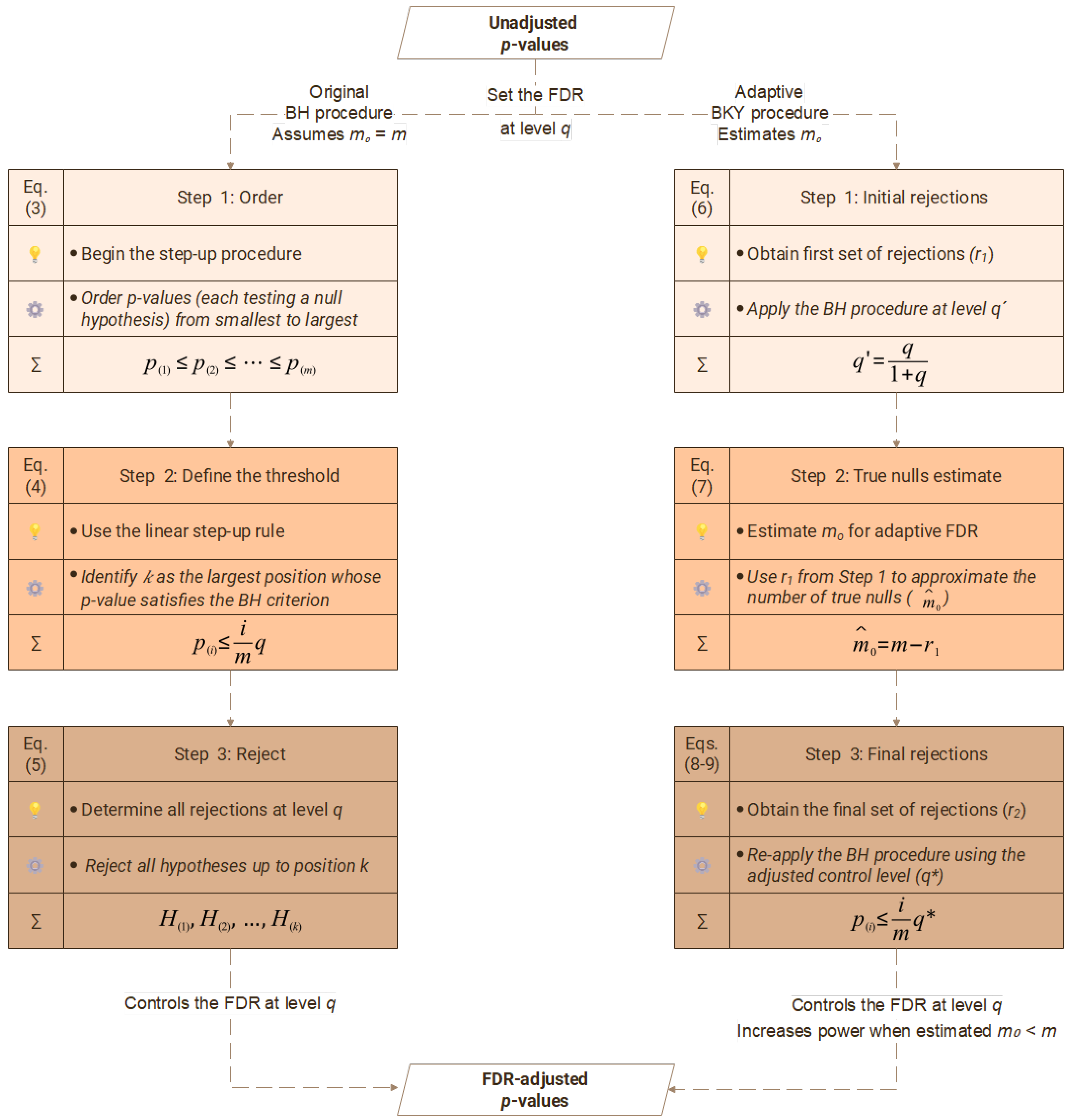
Figure 1. Comparative flowchart of the Benjamini–Hochberg (BH) and Benjamini–Krieger–Yekutieli (BKY) procedures for FDR control. The diagram links each operation to its corresponding equation (Eq./Eqs.), which refers to the equations explained in the main text, and follows the sequence described in the original articles. Light-bulb icons indicate conceptual ideas, gear icons denote computational operations, and the Σ symbol marks the equation or criterion applied at each step. The original BH method assumes that all null hypotheses are true ( m 0 = m ), whereas the adaptive BKY procedure relaxes this assumption by estimating the number of true nulls ( m 0 ), denoted as m ^ 0 . Source: Figure created by the authors.
Mathematics 13 03630 g001
Figure 2. Comparison of rejection thresholds from BH and adaptive BKY procedures under the assumption m0 = 60, illustrating the gain in power achieved by BKY. Source: Figure created by the authors.
Mathematics 13 03630 g002
Figure 3. Global map and histogram of 481,499 raw p-values from the CMK trend test. Source: Figure created by the authors.
Mathematics 13 03630 g003
Figure 4. Comparison of rejection thresholds from FDR-BH and adaptive FDR-BKY procedures (m = 481,499; q = 0.05), showing the relative increase in discoveries achieved by the BKY procedure (π0 = 0.6452). Note: The x-axis represents the rank (k) of 481,499 p-values sorted in ascending order, whilst the y-axis displays the observed p-values. The celestial blue line depicts the corresponding significance threshold for each method. In both panels, blue points indicate discoveries, while grey points represent non-discoveries. A total of 481,499 points is displayed, corresponding to the number of tests performed (m). Source: Figure created by the authors.
Mathematics 13 03630 g004
Figure 5. Number and proportion of significant trends obtained from raw p-values (α = 0.05), FDR-BH (q = 0.05), and adaptive FDR-BKY (q = 0.05) across 481,499 spatially gridded CMK trend tests. Note: In FDR terminology, q is the analogue of the significance level α, and “discoveries” correspond to significant results after multiple testing correction. Source: Figure created by the authors.
Mathematics 13 03630 g005
Figure 6. Spatial distribution of significant trends after multiple testing correction using the linear two-stage adaptive FDR-BKY procedure (q = 0.05). Note: Terminology follows Figure 5. Source: Figure created by the authors.
Mathematics 13 03630 g006
Table 1. Possible outcomes in multiple testing.
H0 Not RejectedH0 RejectedTotal
H0 TrueN0|0
U (true negatives)
N1|0
V (false positives)
Type I errors
m0
(True null hypotheses)
H0 FalseN0|1
T (false negatives)
Type II errors
N1|1
S (true positives)
m1
(False null hypotheses)
TotalmR
(Non-rejections)
R = V + S
(Rejections)
m
(Total tests)
Note: Cross-classification of multiple testing outcomes. The table distinguishes between true and false null hypotheses and the corresponding decisions (rejections and non-rejections), along with the associated error types. Source: Table created by the authors.
Disclaimer/Publisher’s Note: The statements, opinions and data contained in all publications are solely those of the individual author(s) and contributor(s) and not of MDPI and/or the editor(s). MDPI and/or the editor(s) disclaim responsibility for any injury to people or property resulting from any ideas, methods, instructions or products referred to in the content.