Abstract
In the modern age of data enrichment, it has become necessary to incorporate adaptive inference processes into survey-based estimation systems in order to achieve efficient and consistent population summaries. In this work, a new type of data-adaptive approach to the prospective estimation of central tendency under stratified random sampling (StRS) frameworks is presented. The suggested structure takes advantage of the auxiliary information based on locally tuned, non-parametric smoothing plans that dynamically adapt to a heterogeneity of sampled and unsampled domains. The estimator wisely reacts to an intricate pattern of the data, ensured by the application of variable bandwidth functions, stratified weighting plans, which ensure resilience to model misspecification and outlier effects. Substantial Monte Carlo simulations and two empirical studies, i.e., solar radiation data and fish market data, are performed to confirm its performance in a variety of bandwidth and sample size settings. The findings have consistently shown that the suggested adaptive inference mechanism is significantly more precise and stable than traditional estimators, not only when auxiliary expectations are known, but also when they have to be estimated. This study brings into play a flexible, design-conscious framework that connects model-driven estimation with design-driven survey inference, which is of importance in contemporary information-gathering settings of informational diversity and enrichment.
Keywords:
data-adaptive inference; central tendency estimation; stratified random sampling; auxiliary information; non-parametric framework; survey data enrichment; design-based statistical inference MSC:
62D05
1. Introduction
In most complicated surveys, the study population may provide us with data that can be used both during the design phase and during the estimation phase to develop effective approaches to estimating parameters of a finite population, including the population total or the population mean. Such information may be provided by sources such as national census, remote sensing, or information pertaining to the natural resource inventory. Considering the fact that estimation is the key of survey sampling, much attention is paid to the use of supplementary information. The most common method is to have a hypothetical model, which is typically a linear functional form, to represent the relationship between the auxiliary and survey variables. Based on this relationship, the estimator is constructed. It is worth mentioning that employing these estimators relies on prior information about the population parameters’ specific form, which can pose challenges when dealing with multiple variables that require model development, Wu and Sitter [1]. Due to these issues, more emphasis has been placed on non-parametric models that allow for more complex associations between auxiliary and survey variables, Dorfman [2]. It is worth mentioning that the idea of non-parametric modeling was introduced in the works of (Dorfman and Hall [3]).
Non-parametric inference procedures typically differ from model or probability design more sensitively than parametric ones (Nadaraya [4]). The theoretical literature predominantly offers two methods for constructing more efficient estimators: two broad categories of implementation research: model-based and design-based. The model-based approach also assumes that the target population is a sample of the super population model. It is then used to estimate observations for portions of the population not included in the sample to compute finite population parameters (Dorfman and Hall [3]). The first introductory use of non-parametric models in this context was conducted by Nadaraya [4], who argued for the local polynomial regression (LPR) estimator as a broadened kind of regression estimator. A simulation analysis confirmed that the current new estimator was exhibits improved efficiency relative to the other parametric estimators commonly used in the past. Following this, Rueda and Sanchez-Borrego [5] enhanced this line of work with a model-based LPR estimator appropriate for direct probability sampling designs.
Although local polynomial kernel regression can be applied to both continuous and discrete data, its use depends on the type of data being analyzed. Local polynomial model fitting at each point of interest is well suited for continuous data, as it allows a local polynomial function to allocate more weight to nearby points through the use of a kernel function. Furthermore, this approach offers flexible smoothing with relatively minimal global requirements. For discrete data, some adaptations are necessary. As a running example, binary or categorical data can be processed by local polynomial logistic regression, and local generalized linear models (GLMs) with appropriate link functions like Poisson regression are used for count data. It is important to choose the right kernel bandwidth when working with sparse discrete data to ensure optimal performance. For more information on this topic, see [5].
The arithmetic mean is an established measure of statistics and is considered one of the most popular and prominent types of averages, with applications across all fields of science and the arts (Zaman and Iftikhar [6]). For this reason, mean estimation plays a significant role not only in survey sampling but also in many other sectors (Alqudah et al. [7]; Bhushan et al. [8]). For additional information related to mean estimation, readers are referred to the references Bhushan et al. [8] and Koc and Koc [9]. Given these considerations, there is a need to improve mean estimation methods by employing model-based estimation techniques.
This paper focuses on the empirical literature on non-parametric model-based mean estimators. More particularly, in model-based estimation, the model that relates dependent variables to independent variables is formed. Another class of estimation methods builds the fundamental form of the statistical model on which the parameter estimation can be based (Srivastava [10]). Under some assumptions, such models are useful in imputing the non-sampled observations of the dependent variable at the micro and macro levels. When data is collected via a sampling design, then this sampling design too can be brought into the estimation process in the same way as design based estimation. In the same vein, Rueda and Sanchez-Borrego [5] enveloped simple random sampling (SRS), together with an LPR-supported model-based estimator. This estimator reveals several desirable features within the current model-based framework.
It is worthy to note that multiple predictor variables can be handled by multiple LPR (MLPR) by fitting a local polynomial surface rather than simply a local polynomial curve. Due to the curse of dimensionality, MLPR can provide unreliable results. Furthermore, it is crucial to choose appropriate bandwidths for each variable; otherwise, noise variables can be over-smoothed or not smoothed at all. However, with only one predictor, the curse of dimensionality problem is eliminated because the data points are dense in the lower-dimensional space. This means that the kernel function can implement reliable smoothing without inflating the variance much. Furthermore, bandwidth selection is convenient and controllable over a single variable, with no more risk of over-smoothing or under-smoothing.
Despite extensive research, little work has focused on model-based calibration-type mean estimation where calibration constraints leverage auxiliary information. This paper aims to address this gap by using auxiliary information to enhance mean precision through non-parametric model regression. To accomplish this, we implement a model-oriented methodology using a LPR estimator to estimate the non-sampled values of y. The estimator demonstrates favorable properties, as shown by both theoretical and practical analysis. We explore several bandwidth selection methods to identify the optimal one for the new estimator, given its sensitivity to this choice. The proposed procedure serves as a practical alternative to existing estimators. Additionally, the Gaussian function used here displays optimal characteristics for general non-parametric regression.
In recent years, particular concern over the role of quantification and estimation of natural resources, specifically fish stock, has changed the dynamics of aquaculture, fisheries, and fish science fields where advanced estimation techniques have been reported. Fish physical attributes such as size, weight, and potentially shape need to be measured and predicted for the fish stock assessment, markets, and decision making in the fish sector. Therefore, the performance of estimators will be assessed using a real-life dataset of a fish market, which contains information about various fish attributes. This study also includes a dataset that simulates the factors affecting solar ultraviolet (UV) radiation and target labels describing UV risk levels. The purpose of this dataset is to serve as a predictive modeling of UV radiation and risk assessment using tree-based or other machine learning approaches. This research applies both datasets in order to quantify data driven approaches to natural resource estimation, fisheries management, and environmental risk assessment. Lastly, this article also provides an overview of the survey sampling methods in the field of aquaculture and fisheries with special consideration given to the environmental factors, especially UV radiation, that may influence aquatic ecosystems.
The remainder of this article provides comprehensive details on sophisticated mean estimation approaches, particularly within the non-parametric model-based framework, focusing on stratified random sampling (StRS). Section 2 offers preliminary background, introducing specific existing model-based estimators and emphasizing the advantages of non-parametric methods. Section 3 presents an adapted calibrated estimator. Section 4 extends this by employing calibration to further improve the accuracy of estimation in a model-based stratification model. Section 5 provides an insight into the double StRS approach with data characteristics estimated by employing a double-sampling approach to obtain more precise estimates in cases where the average of auxiliary variables is unknown. Section 6 includes simulation studies to evaluate and compare the efficiency of the proposed estimators with others, using varying sample sizes and bandwidth selectors. This extensive analysis demonstrates the practicality and robustness of the derived methods. Finally, conclusions are provided in Section 7.
2. Model-Based Estimator Under StRS
Alomair et al. [11] and Rueda and Sanchez-Borrego [5] suggest that the model-based approach assumes the population can be adequately represented through the predictive model :
For representation under StRS, the prediction model for stratum can be written as
where are with and variance . The term is the smooth function of x. denotes expectation.
Once the sample has been collected, the mean prediction of unobserved values can be written as
where and and with denoting sampled units and for the non-sampled values in the stratum. Further, is the size of stratum, is the size of sample in the stratum, and the correction factor is expressed as . However, the overall population size is N. Note that the initial part of Equation (1) is known. So, the estimation of later part of can be viewed as predicting the mean for data that has not been sampled. If all x values are known, predictions can be straightforwardly made using a regression model, with the surrogate values serving as substitutes for the unobserved values for . However, values are unknown in practice. So, non-parametric kernel regression is utilized to receive estimates for Chambers et al. [12]. Further, this idea is adapted by many researchers including Rueda and Sanchez-Borrego [5]. So, in light of these studies, the traditional model-based estimator under StRS for stratum is
For all the strata, can be written as
where is a conventional stratification weight and represents the total count of strata.
It should be emphasized that in LPR is a generalization of kernel regression and is suitable for use in a wide array of problems. Inspired by the work of Ref. [13], as well as Rueda and Sanchez-Borrego [5], we utilize a kernel-based LPR order estimator to generate predictions for the variable of interest. By defining , where K refers a Gaussian kernel function and h is the bandwidth. For some latest developments about kernel related work, please see Shahzad et al. [14], Ali [15], and Ali et al. [16]. Consequently, the prediction for unknown is
where is the vector with length , , , and .
The estimator can be improved under StRS using a calibration approach. So, in the coming sections, we will extend this work in light of the calibration approach.
3. Adapted Estimator
When supplementary information is used, the accuracy of the estimators of the average value can really improve. As presented by Refs. [17,18], in most actual circumstances, a direct connection is believed to exist between the variable of focal interest Y and the teamed variable X. For example, if education level and income are known to have a direct or ‘causal relation’ (i.e., education level causes income), and it has been proven and expected that people with higher education levels earn more (Smits [19]). A similar example occurs with health-related factors; for instance, there is a direct positive link between activity level and cardiovascular health. Boehm and Kubzansky [20] have noted that an increased level of activity promotes a healthy heart. These common examples show how auxiliary variables are useful in improving the precision of mean estimates.
Calibration estimation is recognized as one of the most efficient techniques for adjusting the initial weights to minimize a specific distance measure, incorporating additional or auxiliary data. Many scholars have discussed calibration weighting within strata to increase efficiency in population parameter estimates. Creating calibration weights requires two main factors: a distance function and associated constraints. Efficient weights for the auxiliary variable can also enhance the study variable. Ref. [21] have advanced calibration-based estimation employing multiple calibration constraints within the survey sampling framework, as discussed by Koyuncu [22], Singh et al. [23], Koyuncu [24], and Sinha et al. [25]. However, the focused mean estimation within the calibrated model based on StRS has not been extensively studied. Building on seminal work such as Koyuncu [24], this article proposes a calibrated model-based mean estimator using StRS from a non-parametric kernel regression perspective.
In light of StRS design, let n and N be the overall sizes of sample and population, and be the sample and population averages of X. be the traditional and calibrated stratification weights. Using these described characteristics, a random sample of size is sampled from a population containing units in stratum, where , and an adapted calibrated estimator is
subject to the constraints
The justification for the use of loss functions in the calibration approach, particularly discussed by Ref. [21], revolves around improving estimation accuracy by modifying the weights assigned to sampled data points. This process minimizes a distance measure between base sampling weights and the post-calibration weights while adhering to calibration constraints. So, a Lagrange function (LF) formulated by including the multipliers , and a Chi-square loss function:
The derivative of w.r.t , by equating zero, provides
Calibrated weights have several significant characteristics including minimum variance reducing bias, and being consistent with the auxiliary information available. The objectives of designing them are to facilitate matching the weighted totals of auxiliary variables in the sample to known population totals so that survey estimates are more accurate. However, calibrated weights are not always guaranteed to be positive. Negative weights may arise, particularly when there are significant differences between the sample and population characteristics or when a specific loss functions are used in the calibration process. However, the problem of negative weights is minimal when using the Chi-square distance in contrast to other distance functions. Because it penalizes extreme deviations more severely, the Chi square distance attempts to keep the weights close to their initial value. Its performance is enhanced by smoother adjustments and decreased likelihood of extreme or negative weights, increasing the calibration stability and relevance.
By substituting and in (6), we receive the following:
By putting in , we receive its final form:
This estimator can be rewritten as
where
Note that the adapted estimator can be converted into the generalized version by choosing different values of . However, for reader simplicity, we currently only use . However, different values of known population characteristics of can be used and the shape of the estimator can be changed accordingly, see Garg and Pachori [26], Pal et al. [27], and Pandy et al. [28].
4. Proposed Estimator
In a model-based approach, the base is built on the so-called superpopulation models ; subsequently, it is assumed that the studied population is an example of the random variables generated under . This model, , takes advantage of information in the population and allows calculation of values that were not directly sampled, especially when determining finite population values such as the mean of Y. Key advantages of this approach include the following:
- 1.
- Model-based theory, also known as prediction theory for survey sampling, is a well rounded theoretical framework for making statistical inferences about finite populations. In this general framework, widely recognized estimators of population parameters can be emerge as predictors under specific models.
- 2.
- This framework is still in line with dominant statistical approaches found in fields like econometrics.
- 3.
- Other fundamental advantages include that for large samples, and under certain distributional assumptions, the model-based results are very close to the design-based inferences.
- 4.
- The variance of the model-based estimators is usually lower than that of the design-based estimators.
The design of the proposed dual calibration structure is aimed at simultaneously depicting the central tendency and relative dispersion of the auxiliary information. The coefficient of variation (CV) constraint is also useful, specifically when the auxiliary variable is heteroscedastic or has considerable inter-strata variance, because this enables the adjusted weights to capture level and scale variance. When the relationship between the study and the auxiliary variables is not necessarily linear, as highlighted by Garg and Pachori [26] and Sinha et al. [25], it is useful to calibrate using both the mean and the CV to greatly reduce MSE. Hence, the CV-based adjustment serves as a scaling procedure that determines the magnification of the efficiency of the estimator by stabilizing the variance across strata.
- So, taking motivation from Refs. [22,24,25,26], the proposed calibrated model-based mean estimator using StRS under non-parametric kernel regression based framework is
By solving Equation (19), we receive
where , and can be found in the Appendix.
Properties of
This proposed estimator has several practical properties:
- First, the estimator is linear, as shown by its functional form, where the estimator incorporates both observed and predicted components of the population, making it a composite measure. The estimator uses a weight factor, say m, which is adjusted based on the influence of non-sampled units.
- Second, the estimator is data-concentrated, requiring knowledge of values for all population elements and necessitating intensive computations.
- Lastly, this estimator does not rely on the design-based probabilities, unlike conventional design-based estimators that typically incorporate these probabilities for inference. Instead, it substitutes them with new weights, say w, determined by the proximity of sample points, aiming to improve model predictiveness and precision. This adjustment aligns the inference process with the conditional principle, focusing on observed sample characteristics rather than average properties across possible samples.
5. Double StRS
Double sampling is especially useful when the population average of X is not known and must be estimated. This is a continuation of Section 5 focusing on a number of cases where this population mean is not available. The present research builds on references (Al-Omari [29]; Alomair and Daraz [30]; Daraz et al. [31]) where the type of sampling changes from a StRS to a two-stage (or double) StRS. In the first stage, the sampling technique used is SRS and in the second stage, the sampling technique used is the StRS. In this context, is the sample size in the first phase for stratum, and is the sample size in the subsequent phase. Attributes of the auxiliary variable in the 1st phase are and and in the 2nd phase within the stratum, both variables characteristics are , and . The traditional model-based estimator for double StRS in the stratum is
For all the strata, can be written as
5.1. Double Adapted Estimator
Th generalized class of estimators under double StRS is given below
subject to the constraints
An LF is formulated by including the multipliers and in the following:
By substituting and in (28), we receive
By putting in , we achieve
This estimator can be rewritten as
where
5.2. Double Proposed Estimator
The proposed estimator under double StRS as given below:
subject to the constraints
An LF formulated by including the multipliers , and :
A derivative of w.r.t , by equating zero, provides
Note that just like the adapted estimator, someone can also generate many other versions of the proposed estimator in light of the references (Garg and Pachori [26]; Pal et al. [27]; Pandey et al. [28]), and by choosing different values of .
Mean estimation techniques are statistically important in fisheries and aquaculture because trends of several important indices of fish stocks including size and growth are important for determination of right harvesting periods and sustainable fishing quotas. The fish market dataset provides an environment to compare the performance of various estimation methods in a real context where modeling of the fish characteristics has direct bearing to the economic returns of fish stocks and therefore viability of the fisheries to support the food needs of the populace. While the point estimates for such stocks based on customary assessments can be useful, applying the calibration approach suggested in this paper, which involves auxiliary information for such datasets, can improve the accuracy of these estimates for the purpose of managing fisheries and aquatic resources by both commercial fishers and regulatory bodies.
6. Numerical Illustration
6.1. Bandwidth Selectors
It is worth noting that and and all the other considered estimators are based on the bandwidth parameter h, which plays a critical role in balancing the bias–variance tradeoff of local polynomial regression. To ensure reliability and consistency of results, we examined the estimator performance under several bandwidth selection strategies. Specifically, bandwidths were chosen using (i) a fixed bandwidth approach, (ii) the direct plug-in method described by Wand and Jones [32], and (iii) two data-driven cross-validation approaches, the Biased and Unbiased methods, as proposed by Scott and Terrell [33]. These methods are known to provide asymptotically consistent bandwidth choices in large samples. Evaluating results across these approaches helped us to assess the effectiveness of estimators (, , , , , and ) under varying bandwidth selection strategies.
6.2. Simulation Experiments
This section’s simulation experiments aim to evaluate the effectiveness and efficiency of the estimators and in comparison to , , , and . For this purpose, three simulated datasets—Sine, Bump, and Jump—were created based on the following regression functions:
where x is uniformly distributed with [0, 1] and error term is independently and identically distributed with zero mean unit standard deviation. For graphical representation, see Figure 1, Figure 2 and Figure 3.
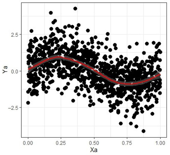
Figure 1.
Sine dataset.
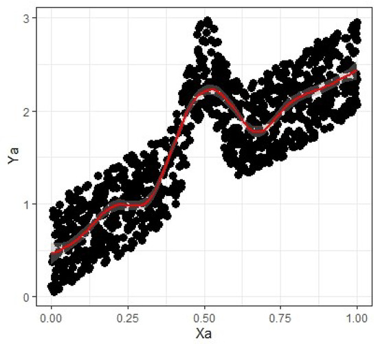
Figure 2.
Bump dataset.
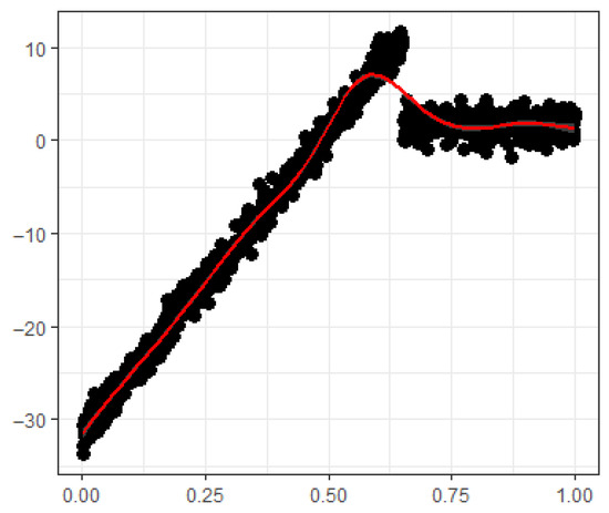
Figure 3.
Jump dataset.
We have considered two simulated populations based on generated datasets, see Equations (43)–(45), under StRS. In the first population, Bump data is considered as stratum-I and Sine data is considered as stratum-II. In the second population, Bump data is considered as stratum-I and Jump data is considered as stratum-II. In each stratum with a size of , inspired by the methodology of Koyuncu [22,24], we draw samples from the specified stratified populations. To enable a fair comparison between the estimators, we collect a range of samples under the StRS scheme. The percentage sizes of these various samples are detailed in Table 1, Table 2, Table 3 and Table 4. The times repeated simulation-experiment-based MSE and PRE results under single and double StRS are provided in Table 1, Table 2, Table 3 and Table 4. For each sample, the numerical values of , , , , , and were obtained. The expressions for MSEs and PREs are
where =, , , and =, , .

Table 1.
MSE using data.
Table 2.
MSE using data.
Table 3.
PRE using data.
Table 4.
PRE using data.
6.3. Real-Life Applications Related to Fisheries and Radiations
The current type of datasets, such as the fish market dataset, are suitable for kernel-based linear polynomial regression (LPR), especially because of its flexibility in modeling complex associations between variables, which is a result of its non-parametric nature. This approach can also be used to analyze the datasets in which factors that influence the solar ultraviolet (UV) radiation are simulated, in order to perform more accurate risk assessment and environmental impact modeling. The utility of kernel regression to estimate the mean and other population parameters is based on the understanding of both fish characteristics and UV exposure risks that can be operationalized within the context of aquaculture, fisheries, and environmental science. These techniques are applied to show how some branches of advanced statistics can be used in many areas to create a theoretical framework that improves the accuracy of fisheries assessments and help aquaculture industry to achieve its sustainability, as well as for ecological monitoring. The combination of fisheries and UV radiation studies using predictive modeling enhances the need for data-driven decision making for resource management and the sustainability of the environment.
Currently, mean estimation based on kernel regression is a part of predictive calibration in fisheries science, as nonlinear dependencies of numerous variables are better modeled with non-parametric than with linear models. Specifically, these models are susceptible to unpredictability and changes in fish characteristics, e.g., weight or length, in a market where biological variability plays a significant role. It is also applicable to predictive modeling methods used on environmental factors which can change not only aquatic ecosystems but the entire ecological balance such as UV (ultraviolet) radiation of the sun. This paper uses the datasets that model the variables of UV radiations and fish market characteristics to analyse how non-parametric regression can be used to enhance the prediction in fisheries science and environmental risk management. In addition to fish stock assessment, these advanced estimation methods assist in the making of decisions in wider scope of aquaculture, fisheries management, and ecological monitoring.
The features of the fish market dataset are as follows: it is a detailed collection of various fish species and their characteristics, organized in a format suitable for analysis. Each row typically captures information about an individual fish and includes multiple physical attributes such as length, height, and width, corresponding to the species listed in that row. The data were obtained from the publicly available website (https://www.kaggle.com/datasets/vipullrathod/fish-market), accessed on 21 October 2024, and approval was not needed. As per the description provided about the data, this data set was collected to develop a predictive model for calculating a fish’s weight from its species and certain standardized measurements. This significant description point motivate us to use this data set as we are also interested in predictive model-based mean estimation.
To stratify the data, the natural grouping variable was the species type, stratum-I represents the height of the Bream species (study variable), and stratum-II represents the width of the Bream species (auxiliary variable). This type of stratification allows for the investigation of heterogeneity across meaningful biological categories.
Solar UV radiation dataset features: a collection of various environmental factors affecting the levels of ultraviolet (UV) radiation and structured for predictive analysis. The rows represent a unique set of atmospheric conditions, each containing multiple other influencing factors (temperature, humidity, ozone levels, and solar angles) and corresponds to specific UV risk levels. The data were obtained from the publicly available website Kaggle, accessed on 22 February 2025, and approval was not needed. As per the description provided about the dataset, it was collected to support the development of predictive models for assessing UV radiation risk based on meteorological and environmental attributes. This dataset is particularly useful for our research, as we are also interested in predictive model-based mean estimation.
Stratum-I was constructed based on low UV risk levels, and stratum-II on moderate UV risk levels, which are realistic environmental groupings that can be compared. The study variable in this context is solar radiation intensity, which plays a critical role in evaluating UV exposure and its potential impact.
Accordingly, both examples are illustrative and comparative, and these approaches align with the standard pseudo-population principle used in simulation-based survey methodology. The results of the fisheries and radiations data analysis are presented in Table 5, Table 6, Table 7 and Table 8. The auxiliary variable x is generated using uniform distribution [0, 1] as per following the guide lines of Rueda and Sanchez-Borrego [5], Younis and Shabbir [34], and Qureshi et al. [35]. The results of the fish market data analysis are presented in Table 5 and Table 6.
Table 5.
MSE using fish data.
Table 6.
MSE using radiations data.
Table 7.
PRE using fish data.
Table 8.
PRE using radiations data.
6.4. Interpretation
Table 1 and Table 2 illustrate the results where the basic regression estimator () and the adapted estimator () both underperform the predictive mean estimator () in terms of lowering their MSE values with respect to different sample sizes and bandwidth selectors. Secondly, the double StRS is slightly more accurate than the single-stage version StRS, as confirmed by smaller values of MSE for the double (), (), and () estimators. Moreover, the bandwidth selection plays a critical role in the accuracy of the estimators, and especially data-driven bandwidth selectors (dpik, bcv, and ucv) always result in lower MSE than fixed ones , and dpik performs the best. The same pattern of results can be seen in Table 3 and Table 4.
Table 5 and Table 6 present the Mean Squared Error (MSE) values obtained from the fisheries and radiations datasets under both stratified random sampling (StRS) and double stratified random sampling (double StRS). The estimators assessed include , , and , along with their double stratified versions (, , and ). The data was analyzed across different sample sizes ( and ) and bandwidth selectors (). The results indicate that the predictive mean estimator () and its double StRS version () outperform the basic and adapted regression estimators in terms of MSE reduction across all scenarios. The same pattern of results can be seen in Table 7 and Table 8.
Moreover, the sensitivity analysis was conducted in a detailed manner to determine the soundness of the proposed estimators in different experimental conditions. In particular, the analysis has taken into consideration the impact of bandwidth variation, i.e., changing the fixed bandwidth values and , as well as the impact of sample size variation and . Computed values of PRE at varying sample sizes serve as an indicator of sensitivity, demonstrating the effect of variation of a data scale on the estimators. The comparative results showed that the MSE-based PRE variations were very small with either under- or over-smoothing to extreme, but the general efficiency patterns and the ranking of the proposed estimators were steady. All these findings are reassuring regarding the strength and stability of the proposed calibration-based framework across various data-driven bandwidth selectors and sample sizes.
As shown, the PRE values for all proposed estimators are above 100, demonstrating their enhanced performance compared to other estimators. Although this conclusion is drawn from our simulation study, we believe that similar outcomes would be likely in other scenarios as well.
7. Conclusions
The purpose of this work is to build a framework using a non-parametric model-based estimator, kernel regression, and calibration for average estimation. To improve the precision of the average with a given set of calibrated weights, the proposed method is based on StRS. This estimator was confirmed to be superior to traditional and model-based adapted estimators through simulations and real datasets from the fish market and solar UV radiation datasets. The fish market dataset in the field of aquaculture and fisheries was used, where fish characteristics estimation is critical for stock control and market evaluation, and the results of this method were shown to be effective. Similarly, when applied to environmental science on the solar UV radiation dataset, the method showed applicability in the modeling and the assessment of solar radiation intensity and UV risk levels. It has been demonstrated that local polynomial kernel regression and calibration, utilizing the known or estimated calibration function, enhance the estimation efficiency. This improvement is further enhanced when auxiliary variables are included. The relative efficiency of predictions showed that the proposed methodology could be used not only in fisheries science, but also in the case of prediction of the UV radiation risk, making it a valuable technique. The kernel regression-based predictive calibration method is flexible, robust, and may be used for non-parametric mean estimation in survey sampling, resource management, and environmental risk assessment.
Author Contributions
Conceptualization, H.M.A. and M.M.A.; Methodology, H.M.A. and M.M.A.; Software, H.M.A. and M.M.A.; Validation, H.M.A.; Formal analysis, H.M.A.; Investigation, H.M.A.; Resources, H.M.A.; Data curation, H.M.A.; Writing—original draft, H.M.A. and M.M.A.; Writing—review & editing, H.M.A. and M.M.A.; Visualization, H.M.A. and M.M.A.; Supervision, H.M.A.; Project administration, H.M.A.; Funding acquisition, H.M.A. All authors have read and agreed to the published version of the manuscript.
Funding
The authors extend their appreciation to the Deanship of Scientific Research and Libraries in Princess Nourah bint Abdulrahman University for funding this research work through the Program for Supporting Publication in Top-Impact Journals, Grant No. (SPTIF-2025-6).
Data Availability Statement
All the relevant data information is available within the manuscript.
Conflicts of Interest
The authors declare no conflicts of interest.
Correction Statement
The article has been republished with a minor correction to the Funding statement. This change does not affect the scientific content of the article.
Appendix A
References
- Wu, C.; Sitter, R.R. A model-calibration approach to using complete auxiliary information from survey data. J. Am. Stat. Assoc. 2001, 96, 185–193. [Google Scholar] [CrossRef]
- Dorfman, A.H. Nonparametric regression for estimating totals in finite populations. In Proceedings of the Section on Survey Research Methods; American Statistical Association: Alexandria, VA, USA, 1992; pp. 622–625. [Google Scholar]
- Dorfman, A.H.; Hall, P. Estimators of the finite population distribution function using nonparametric regression. Ann. Stat. 1993, 21, 1452–1475. [Google Scholar] [CrossRef]
- Nadaraya, E.A. On estimating regression. Theory Probab. Its Appl. 1964, 9, 141–142. [Google Scholar] [CrossRef]
- Rueda, M.; Sanchez-Borrego, I.R. A predictive estimator of finite population mean using nonparametric regression. Comput. Stat. 2009, 24, 1–14. [Google Scholar] [CrossRef]
- Zaman, T.; Iftikhar, S. A New Logarithmic ratio type estimator of population mean for simple random sampling: A simulation study. J. Sci. Arts 2023, 23, 839–848. [Google Scholar] [CrossRef]
- Alqudah, M.A.; Zayed, M.; Subzar, M.; Wani, S.A. Neutrosophic robust ratio type estimator for estimating finite population mean. Heliyon 2024, 10, e28934. [Google Scholar] [CrossRef]
- Bhushan, S.; Kumar, A.; Alrumayh, A.; Khogeer, H.A.; Onyango, R. Evaluating the performance of memory type logarithmic estimators using simple random sampling. PLoS ONE 2022, 17, e0278264. [Google Scholar] [CrossRef]
- Koc, T.; Koc, H. A new class of quantile regression ratio-type estimators for finite population mean in stratified random sampling. Axioms 2023, 12, 713. [Google Scholar] [CrossRef]
- Srivastava, S.K. Predictive estimation of finite population mean using product estimator. Metrika 1983, 30, 93–99. [Google Scholar] [CrossRef]
- Alomair, A.M.; Shahzad, U.; Al-Noor, N.H.; Zhu, H. Probability weighted moments and family of non-parametric regression estimators. Maejo Int. J. Sci. Technol. 2025, 19, 160–170. [Google Scholar]
- Chambers, R.L.; Dorfman, A.H.; Wehrly, T.E. Bias robust estimation in finite populations using nonparametric calibration. J. Am. Stat. Assoc. 1993, 88, 268–277. [Google Scholar] [CrossRef]
- Breidt, F.J.; Opsomer, J.D. Local polynomial regression estimators in survey sampling. Ann. Stat. 2000, 28, 1026–1053. [Google Scholar] [CrossRef]
- Shahzad, U.; Ahmad, I.; Almanjahie, I.M.; Al–Noor, N.H.; Hanif, M. Adaptive Nadaraya-Watson kernel regression estimators utilizing some non-traditional and robust measures: A numerical application of British food data. Hacet. J. Math. Stat. 2023, 52, 1425–1437. [Google Scholar] [CrossRef]
- Ali, T.H. Modification of the adaptive Nadaraya-Watson kernel method for nonparametric regression (simulation study). Commun. Stat. Simul. Comput. 2022, 51, 391–403. [Google Scholar] [CrossRef]
- Ali, T.H.; Hayawi, H.A.A.M.; Botani, D.S.I. Estimation of the bandwidth parameter in Nadaraya-Watson kernel non-parametric regression based on universal threshold level. Commun. Stat. Simul. Comput. 2023, 52, 1476–1489. [Google Scholar] [CrossRef]
- Shahzad, U.; Ahmad, I.; Alshahrani, F.; Almanjahie, I.M.; Iftikhar, S. Calibration-based mean estimators under stratified median ranked set sampling. Mathematics 2023, 11, 1825. [Google Scholar] [CrossRef]
- Koc, H.; Tanis, C.; Zaman, T. Poisson regression-ratio estimators of the population mean under double sampling, with application to COVID-19. Math. Popul. Stud. 2022, 29, 226–240. [Google Scholar] [CrossRef]
- Smits, J. Social closure among the higher educated: Trends in educational homogamy in 55 countries. Soc. Sci. Res. 2003, 32, 251–277. [Google Scholar] [CrossRef]
- Boehm, J.K.; Kubzansky, L.D. The heart’s content: The association between positive psychological well-being and cardiovascular health. Psychol. Bull. 2012, 138, 655. [Google Scholar] [CrossRef]
- Deville, J.C.; Sarndal, C.E. Calibration estimators in survey sampling. J. Am. Stat. Assoc. 1992, 87, 376–382. [Google Scholar] [CrossRef]
- Koyuncu, N. New difference-cum-ratio and exponential type estimators in median ranked set sampling. Hacet. J. Math. Stat. 2016, 45, 207–225. [Google Scholar] [CrossRef]
- Singh, S.; Horn, S.; Yu, F. Estimation variance of general regression estimator: Higher level calibration approach. Surv. Methodol. 1998, 48, 41–50. [Google Scholar]
- Koyuncu, N. Calibration estimator of population mean under stratified ranked set sampling design. Commun. Stat. Theory Methods 2018, 47, 5845–5853. [Google Scholar] [CrossRef]
- Sinha, N.; Sisodia, B.V.S.; Singh, S.; Singh, S.K. Calibration approach estimation of the mean in stratified sampling and stratified double sampling. Commun. Stat. Theory Methods 2017, 46, 4932–4942. [Google Scholar]
- Garg, N.; Pachori, M. Use of coefficient of variation in calibration estimation of population mean in stratified sampling. Commun. Stat. Theory Methods 2019, 49, 5842–5852. [Google Scholar] [CrossRef]
- Pal, A.; Varshney, R.; Yadav, S.K.; Zaman, T. Improved memory-type ratio estimator for population mean in stratified random sampling under linear and non-linear cost functions. Soft Comput. 2024, 28, 7739–7754. [Google Scholar] [CrossRef]
- Pandey, M.K.; Singh, G.N.; Zaman, T.; Al Mutairi, A.; Mustafa, M.S. Improved estimation of population variance in stratified successive sampling using calibrated weights under non-response. Heliyon 2024, 10, e27738. [Google Scholar] [CrossRef]
- Al-Omari, A.I. Ratio estimation of the population mean using auxiliary information in simple random sampling and median ranked set sampling. Stat. Probab. Lett. 2012, 82, 1883–1890. [Google Scholar] [CrossRef]
- Alomair, M.A.; Daraz, U. Dual Transformation of Auxiliary Variables by Using Outliers in Stratified Random Sampling. Mathematics 2024, 12, 2839. [Google Scholar] [CrossRef]
- Daraz, U.; Alomair, M.A.; Albalawi, O.; Al Naim, A.S. New techniques for estimating finite population variance using ranks of Auxiliary Variable in Two-Stage Sampling. Mathematics 2024, 12, 2741. [Google Scholar] [CrossRef]
- Wand, M.P.; Jones, M.C. Kernel Smoothing; Chapman and Hall: London, UK, 1995. [Google Scholar]
- Scott, D.W.; Terrell, G.R. Biased and unbiased cross-validation in density estimation. J. Am. Stat. Assoc. 1987, 82, 1131–1146. [Google Scholar] [CrossRef]
- Younis, F.; Shabbir, J. Estimation of general parameters under stratified adaptive cluster sampling based on dual use of auxiliary information. Sci. Iran. 2021, 28, 1780–1801. [Google Scholar] [CrossRef]
- Qureshi, M.N.; Khalil, S.; Hanif, M. Joint influence of exponential ratio and exponential product estimator for the estimation clustered population mean in adaptive cluster sampling. Adv. Appl. Stat. 2018, 53, 13–28. [Google Scholar] [CrossRef]


Disclaimer/Publisher’s Note: The statements, opinions and data contained in all publications are solely those of the individual author(s) and contributor(s) and not of MDPI and/or the editor(s). MDPI and/or the editor(s) disclaim responsibility for any injury to people or property resulting from any ideas, methods, instructions or products referred to in the content. |
© 2025 by the authors. Licensee MDPI, Basel, Switzerland. This article is an open access article distributed under the terms and conditions of the Creative Commons Attribution (CC BY) license (https://creativecommons.org/licenses/by/4.0/).