A Biased Random-Key Genetic Algorithm for Maximum Flow with Minimum Labels

Abstract

In this work, we propose a novel Biased Random-Key Genetic Algorithm (BRKGA) to solve the Maximum Flow with Minimum Number of Labels (MF-ML) problem, a challenging NP-Complete variant of the classical Maximum Flow problem defined on graphs in which arcs have both capacities and labels assigned. Labels give a qualitative characterization of each connection, in contexts where a solution that is as homogeneous as possible is sought. The MF-ML problem aims to maximize the flow from a source to a sink on a capacitated network while minimizing the number of distinct arc labels used, a modeling framework with applications such as water purification in distribution systems. Our proposed algorithm encodes solutions as random-key vectors, which are decoded into feasible solutions. The BRKGA demonstrates superior performance when compared to a Skewed Variable Neighborhood Search (VNS) approach previously proposed to solve MF-ML. In particular, on the largest considered graphs, BRKGA-MFML outperformed VNS in 55 out of 81 scenarios, with an average improvement per scenario that reaches 7.18%.

1. Introduction

Edge or arc-labeled graphs provide a robust framework for designing and evaluating networks that capture the complex and varied nature of many physical infrastructures in the real world. While weights provide a quantitative characterization of each connection, labels (sometimes also called colors) give a qualitative one, proving useful when there is a need to discriminate among different types of connections.

A significant class of problems aims to find a solution (such as a path, a spanning tree, or a network flow) that is as homogeneous as possible in terms of its labels. Two primary paradigms exist for pursuing this objective: one focuses on minimizing the total number of labels used, while the other focuses on the costs or rules associated with transitioning between different labels [1]. Here, we focus on the former paradigm, which is critical when the presence of each additional label incurs a fixed cost or adds complexity to the overall system. Problem examples from the literature include the following:

• Minimum Label Spanning Tree finds a spanning tree that uses the minimum number of distinct labels [2,3,4,5,6]. Variants where a label set is associated to each edge have also been proposed [7,8].
• Label s-t Cut finds a subset of labels such that the removal of all edges with these labels from the graph disconnects a source from a sink node. The objective can be finding a minimum [9] or maximum [10] number of labels. In the colorful [10] variant, all labels need to be used.
• Maximum Flow with Minimum Number of Labels finds a flow of the maximum value using the minimum number of labels [11].
• Labeled Shortest Path identifies a path between two nodes that has the fewest labels. This is a variation of the shortest path problem where the length of a path is given by the number of distinct labels on its edges [12,13,14].
• Labeled Traveling Salesman Problem looks for a Hamiltonian cycle with the minimum number of different labels [15,16,17].
• Labeled disjoint s-t Paths: finds link-disjoint paths that use the minimum number of total labels. The two-disjoint-path problem is faced in [14], while the maximum number of disjoint uni-color (that is, single-label) paths is studied in [18].

In this paper, we present a Biased Random-Key Genetic Algorithm (BRKGA) metaheuristic algorithm to solve the Maximum Flow with Minimum Number of Labels (MF-ML) problem. We call the proposed adaptation of the BRKGA to this problem the Biased Random-Key Genetic Algorithm for the Maximum Flow with Minimum Labels (BRKGA-MFML). The problem was first introduced by [11], who showed it was NP-Complete, and a Skewed VNS metaheuristic was proposed for its resolution. A practical application of the problem concerning the purification of water in distribution systems is also discussed.

BRKGAs [19] are a class of genetic algorithms applied successfully to several optimization problems, such as routing problems [20,21], scheduling problems [22,23], and the Knapsack Problem with Forfeit Sets [24]. While the No Free Lunch theorem [25] states that no algorithm can be universally superior for all problem classes, the strong performance of BRKGA for combinatorial optimization makes it a suitable candidate to solve MF-ML. Indeed, in this work, we demonstrate that it can outperform the VNS algorithm proposed in [11].

The work is organized as follows. The problem is formally defined in Section 2. Two mathematical formulations are presented in Section 3. The proposed BRKGA-MFML algorithm is presented in detail in Section 4, and its performance tests are analyzed in Section 5.

Final discussions are contained in Section 6.

2. Basic Notations and Definitions

Let $G=(N,A,L)$ be a directed arc-labeled graph, defined on a set of nodes N, a set of arcs A, and a set of labels L. We distinguish two special nodes: a source $s\in N$ and a destination $t\in N$. Each arc $(i,j)\in A$ is associated with a capacity $u_{ij}\ge 0$ and a label $l_{ij}\in L$.

A feasible flow x is defined as a function $x:A\to {\mathbb{R}}^{+}$ that assigns a flow value $x_{ij}$ to each arc, satisfying the classic capacity and conservation constraints. The total value of the flow, denoted by $f\ge 0$, is the net flow coming out of the source (or, equivalently, coming into the sink). We define $G^x=(N,A^x,L^x,f)$ as the subgraph induced by a flow x and its value f, where $A^x\subseteq A$ contains only the set of arcs with a positive flow $A^x=\{(i,j)\in A|x_{ij}>0\}$, and $L^x$ is the set of labels corresponding to the arcs in $A^x$, that is, $L^x=\left\{l_{ij}\right|(i,j)\in A^x\}$. We note that a feasible flow can exist for any value f in the range $[0,f^{max}]$, where $f^{max}$ is the maximum possible flow from s to t.

Among all possible flow configurations, the Maximum Flow with Minimum Number of Labels (MF-ML) problem introduced by [11] looks for a feasible flow x that not only achieves the maximum flow value $f=f^{max}$ but also minimizes $z=|L^x|$. Let $z^{*}$ denote the optimal objective function value.

With these notations in place, we are now ready to formalize two important concepts introduced in [11]: the “necessary label (NL)” and the “necessary node (NN)”. A label $k\in L$ is defined as a necessary label (NL) if its removal from the network decreases the maximum achievable flow from $f^{max}$ to $f_k$ with $f_k<f^{max}$. This concept is formalized as follows:

Definition 1

(Necessary label (NL) [11]). Given a network $G=(N,A,L)$ allowing a maximum flow $f^{max},$ with source $s\in N$, sink $t\in N$, and label set L, a label $k\in L$ is a necessary label if and only if the induced subgraph obtained by removing label k from set L (that is, $G_{L\setminus \left\{k\right\}}=\{N,A_k,L\setminus \left\{k\right\}\}$, with $A_k=\{(i,j)\in A:l_{ij}\in L\setminus \left\{k\right\}\}$) does not allow a maximum flow of value $f^{max}$, but rather a strictly lower maximum flow $f_k$ ($f_k<f^{max}$).

Let $S_{NL}$ denote the set of all necessary labels. This set contains all labels $k\in L$ that satisfy the conditions of Definition 1.

Analogously, a node $i\in N\setminus \{s,t\}$ is defined as a necessary node (NN) if its removal from the network decreases the maximum achievable flow from $f^{max}$ to $f_i$, with $f_i<f^{max}$. Formally, a necessary node is defined as follows.

Definition 2

(Necessary Node (NN) [11]). Given a network $G=(N,A,L)$ allowing a maximum flow $f^{max},$ with source $s\in N$, sink $t\in N$, and label set L, a node $i\in N\setminus \{s,t\}$ is a necessary node if and only if the induced subgraph obtained by removing node i from N (that is, $G_{N\setminus \left\{i\right\}}=\{N\setminus \left\{i\right\},A^i,L\}$, where $A^i=\{(u,v)\in A:u,v\in N\setminus \left\{i\right\}\}$) does not allow a maximum flow of value $f^{max}$, but rather a strictly lower maximum flow $f_i$ ($f_i<f^{max}$). The underflow associated with node i is defined as $f_i^{-}=f^{max}-f_i$.

Similarly, we denote the set of necessary nodes by $S_{NN}$. This set contains all nodes $i\in N\setminus \{s,t\}$ that satisfy the conditions of Definition 2. Note that, by definition, $f_i^{-}>0$$\forall i\in S_{NN}$.

3. Mathematical Formulations

In this section, we present Mixed-Integer Linear Programming (MILP) models, ILP1 and ILP2, which were originally introduced in [11] and are further refined here. These formulations aim to address the Maximum Flow with Minimum Number of Labels (MF-ML) problem.

Let us consider a flow x of maximum value, and its induced subgraph and flow value $G^x=(N,A^x,L^x,f^{max})$. We introduce a binary variable $y_k$ for each label $k\in L$, equal to 1 if the label belongs to the label subset $L^x$ induced by flow x (i.e., $k\in L^x$), and 0 otherwise.

$$\begin{array}{c}\hfill \mathbf{ILP}\mathbf{1}:\\ \hfill z^{*}:=& min\sum _{k\in L}{y}_k\hfill \end{array}$$

$$\begin{array}{cc}& \sum _{j:(s,j)\in A}{x}_{sj}=f^{max}\hfill \end{array}$$

(1)

$$\begin{array}{cc}& \sum _{h:(h,t)\in A}{x}_{ht}=f^{max}\hfill \end{array}$$

(2)

$$\begin{array}{cc}& \sum _{j:(i,j)\in A}{x}_{ij}-\sum _{h:(h,i)\in A}{x}_{hi}=0\forall i\in N\setminus \{s,t\}\hfill \end{array}$$

(3)

$$\begin{array}{cc}& M·y_k\ge \sum _{(i,j)\in A:l(i,j)=k}{x}_{ij}\forall k\in L\hfill \end{array}$$

(4)

$$\begin{array}{cc}& 0\le x_{ij}\le u_{ij}\forall (i,j)\in A\hfill \end{array}$$

(5)

$$\begin{array}{cc}& y_k\in \{0,1\}\forall k\in L\hfill \end{array}$$

(6)

The objective function aims to minimize the number of labels $|L^x|$ used for sending the flow x of value $f^{max}$ from the source s to the sink t. Constraints (1)–(3) are the standard flow conservation equations that must hold for a feasible flow.

They ensure that for the source node, the outgoing flow is equal to the ingoing flow at the sink node, which is of value $f^{max}$, and that for all intermediate nodes ($i\in N\setminus \{s,t\}$), to ensure balance, the total ingoing flow equals the total outgoing flow. Constraints (4) force $y_k$ to 1 whenever there is any positive flow in subgraph $G^x$ with label $k\in L^x$. M represents a sufficiently large constant, which ensures that if any flow is sent on an arc with label k, $y_k$ is activated. Since M must be an upper bound on the cumulative flow traversing the edges of a given color, a valid value for M is $\left|A\right|·f^{max}$, which was used in our tests. The capacity constraints (5) ensure that flow $x_{ij}$ on arc $(i,j)$ does not exceed its capacity and remains non-negative. Lastly, constraints (6) define $y_k$ as binary decision variables for labels $k\in L$.

Formulation ILP2 is a modification of ILP1 designed to incorporate insights derived from the problem structure, specifically through the concepts of necessary labels and necessary nodes, as defined in Section 2.

$$\begin{array}{c}\hfill \mathbf{ILP}\mathbf{2}:\\ \hfill z^{*}:=& |S_{NL}|+min\sum _{k\in L\setminus S_{NL}}{y}_k\hfill \\ \hfill & \left(1\right),\left(2\right),\left(3\right),\left(5\right)\hfill \end{array}$$

$$\begin{array}{cc}& M·y_k\ge \sum _{(i,j)\in A:l(i,j)=k}{x}_{ij}\forall k\in L\setminus S_{NL}\hfill \end{array}$$

(7)

$$\begin{array}{cc}& \sum _{j:(i,j)\in A}{x}_{ij}\ge f_i^{-}\forall i\in S_{NN}\hfill \end{array}$$

(8)

$$\begin{array}{cc}& \sum _{j:(j,i)\in A}{x}_{ji}\ge f_i^{-}\forall i\in S_{NN}\hfill \end{array}$$

(9)

$$\begin{array}{cc}& y_k\in \{0,1\}\forall k\in L\setminus S_{NL}.\hfill \end{array}$$

(10)

The objective function explicitly accounts for the number of necessary labels $|S_{NL}|$, which are known to be part of any maximum flow solution. Therefore, the minimization focuses on the labels that are not necessary, that is, labels in $L\setminus S_{NL}$. Constraints (1), (2), (3) are the same as ILP1, ensuring that the maximum flow $f^{max}$ is achieved. Logical constraints (7) are also equivalent to (4); however, they are specifically applied only on labels in $L\setminus S_{NL}$. The value of M in (7) is the same as that discussed for ILP1. Constraints (5) as in ILP1 are capacity constraints for the arcs.

Constraints (8) and (9) represent flow requirements for necessary nodes. By definition, we know that the removal of a node $i\in S_{NN}$ would reduce the maximum flow $f^{max}$ of a quantity $f_i^{-}$; it follows that a flow equal to at least $f_i^{-}$ must pass through i in any feasible solution. Therefore, for each necessary node, we impose both the outgoing and ingoing flow to be greater than or equal to the corresponding underflow value. Finally, binary decision variables (10) indicate which non-necessary labels are chosen.

An improved formulation can be derived by relaxing the standard flow-balance constraints for nodes in $N\setminus \{s,t\}$ (3):

This relaxation replaces the strict equality constraint with deviation of up to $\Delta$.

$$\begin{array}{ccc}\hfill \sum _{j:(i,j)\in A}{x}_{ij}-\sum _{h:(h,i)\in A}{x}_{hi}& \ge -\Delta \hfill & \hfill \hspace{1em}\hspace{1em}\forall i\in N\setminus \{s,t\}\end{array}$$

(11)

$$\begin{array}{ccc}\hfill \sum _{j:(i,j)\in A}{x}_{ij}-\sum _{h:(h,i)\in A}{x}_{hi}& \le \Delta \hfill & \hfill \hspace{1em}\hspace{1em}\forall i\in N\setminus \{s,t\}\end{array}$$

(12)

4. Biased Random-Key Genetic Algorithm

In this section, we present the Biased Random-Key Genetic Algorithm (BRKGA) that we developed to solve the BRKGA-MFML problem. Like other genetic algorithms, BRKGAs are inspired by the evolutionary process of a population of individuals through several generations, and contain mechanisms mimicking the occurrence of mutations, crossover (generation of offspring from parent individuals), and natural selection. Each individual (also called a chromosome) represents an encoding of the considered optimization problem, and its fitness to the environment is evaluated through an appropriate fitness function, usually corresponding (as in our case) to the objective function of the problem.

In BRKGAs, chromosomes consist of fixed-size vectors of real numbers in the interval $[0,1]$ (random keys); their elements are individually called genes, and the specific random key assigned to each gene within a chromosome is also called an allele.

To design a BRKGA, it is essential to define an appropriate decoder operator, that is, a deterministic function that assigns a feasible solution to each possible chromosome. Once the chromosomes are decoded, it is possible to compute their fitness and therefore to rank them from least fit to most fit.

In the following, we describe our algorithm in detail. In particular, Section 4.1 presents the scheme of the algorithm, while the chromosome structure and the decoder function are described in detail in Section 4.2 and Section 4.3, respectively.

4.1. Algorithm Overview

As mentioned, BRKGAs evolve a population (set of chromosomes) over multiple generations, where each generation corresponds to an iteration of the algorithm, until some stopping condition is met. The population size $popsize\ge 2$ remains constant throughout the generations, and the starting population is composed of randomly generated chromosomes.

Given the g-th population ($g\ge 1)$, the $g+1$-th population is constructed as follows, where $0<p_e<1$, $0<p_m<1$ (with $p_e+p_m<1$), and $0.5<{\rho }_e<1$ are three typical parameters of BRKGAs:

• The best $p_e·popsize$ individuals (according to the fitness function) of the g-th generation, called the elite, are carried over to the $g+1$-th population.
• $p_m·popsize$ new random chromosomes (called mutants) are included in the $g+1$-th population to add diversification.
• Finally, the remaining $(1-p_e-p_m)·popsize$ chromosomes are generated through a crossover operator. The generation of each child chromosome through crossover works as follows: a random elite chromosome and a random non-elite one from population g are first chosen as parents. The allele assigned to each gene of the child will be equal to the corresponding allele in the elite parent with probability ${\rho }_e$, and to the corresponding allele of the other parent otherwise.

The introduction of mutants in each generation favors the exploration of diverse regions of the search space, while the randomized crossover (biased towards elite individuals) allows us to explore solutions close to the most promising ones.

We adopted two different stopping conditions. The algorithm ends as soon as one of the two is reached. The first condition is a maximum number of iterations $max\_generations\ge 1$. The second condition is related to a maximum number of consecutive iterations without improving the best overall solution (incumbent solution) and is controlled by two integer parameters, $max\_no\_imp\ge 1$ and $total\_no\_imp\ge 1$.

Pseudocode of BRKGA-MFML is given in Algorithm 1. The procedure initializes population $POP$ with random chromosomes, decodes them building the corresponding set of solutions $\mathcal{S}$, and saves incumbent solution $S^{*}$, that is, the best solution in $S$ (lines 4–6). Note that with $DecodeChromosomes$, we represent the execution of the decoder operator on each element of $POP$. The decoder makes use of two parameters $\alpha$ and $\beta$, as well as a hash table. They are used in the completion (see Section 4.3.2) and cleaning (see Section 4.3.4) steps of the decoder and to avoid unnecessary computations (see Section 4.3.5).

Lines 7–29 represent the main loop of the algorithm, executed at most $max\_generations$ times. The population is updated with new individuals as previously described, and the decoder is used to find the corresponding new solutions (lines 8–12). If the current best solution is improved, $S^{*}$ is updated, and the counter of iterations since the last improvement $g\_no\_imp$ is reset to 0; otherwise, its value is increased by 1 (lines 13–18). The current iteration ends, unless $g\_no\_imp$ reached $max\_no\_imp$. In this case, if we did not already encounter $max\_no\_imp$ iterations without improvements $total\_no\_imp$ times, we reset $g\_no\_imp$ to 0. Otherwise, the algorithm terminates, returning the best solution found $S^{*}$ (line 24). The incumbent solution is also returned if we end the main loop, having executed it $max\_generations$ times (line 28).

Algorithm 1 BRKGA-MFML algorithm

Input:  Graph G, integer parameters $\alpha \ge 1$, $popsize\ge 2$, $max\_generations\ge 1$$max\_no\_imp\ge 1$, $total\_no\_imp\ge 1$, continuous parameters $0<\beta \le 1$, $0<p_e<1$, $0<p_m<1$, $0.5<{\rho }_e<1$ Output:  Best found solution $S^{*}$   1: $g\_no\_imp\leftarrow 0$   2: $n\_max\_no\_imp\leftarrow 0$   3: $HashTable\leftarrow \varnothing$   4: $POP\leftarrow RandomPopulation\left(popsize\right)$   5: $\mathcal{S}\leftarrow DecodeChromosomes(G,POP,\alpha ,\beta ,HashTable)$   6: $S^{*}\leftarrow BestSol\left(S\right)$   7: for $g=1\to max\_generations$ do   8:    $PO{P}^{\prime }\leftarrow Elite(POP,popsize,p_e)$   9:    $PO{P}^{\prime }\leftarrow Mutants(popsize,p_m)$ 10:    $PO{P}^{\prime }\leftarrow Crossover(POP,1-p_e-p_m,{\rho }_e)$ 11:    $POP\leftarrow PO{P}^{\prime }$ 12:    $\mathcal{S}\leftarrow DecodeChromosomes(G,POP,\alpha ,\beta ,HashTable)$ 13:    if $Fit\left(BestSol\left(S\right)\right)<Fit\left(S^{*}\right)$ then 14:        $g\_no\_imp\leftarrow 0$ 15:        $S^{*}\leftarrow BestSol\left(S\right)$ 16:    else 17:        $g\_no\_imp\leftarrow g\_no\_imp+1$ 18:    end if 19:    if $g\_no\_imp==max\_no\_imp$ then 20:        if $n\_max\_no\_imp<total\_no\_imp$ then 21:            $g\_no\_imp\leftarrow 0$ 22:            $n\_max\_no\_imp\leftarrow n\_max\_no\_imp+1$ 23:        else 24:            return $S^{*}$ 25:        end if 26:    end if 27: end for 28: return $S^{*}$

4.2. Chromosome Structure

As mentioned, in BRKGAs, each chromosome is a vector of real numbers in the interval $[0,1]$, and it encodes a feasible solution for the studied problem. In the case of MFML, a feasible solution corresponds to a subset of labels $S\subseteq L$ such that their arcs allow a flow of value $f^{max}$ in G. Therefore, each gene within a chromosome is associated with a label.

As discussed, no decision can be made for necessary labels, since they are included in each feasible solution by definition. BRKGA-MFML focuses, therefore, on the optimal identification of labels in $\mathcal{L}=L\setminus S_{NL}$, and each chromosome will be composed of $\left|\mathcal{L}\right|$ genes. Therefore, when discussing a BRKGA-MFML solution, we will focus on the identification of a label subset $S\subseteq \mathcal{L}$, such that the labels in $S\cup S_{NL}$ allow a flow $f^{max}$ in G.

4.3. Decoder Operator

Let $\mathrm{\Gamma }\in POP$ be a chromosome of the current population, and let $\mathrm{\Gamma }\left[k\right]$ be the allele (chromosome value) associated with the non-necessary label $k\in \mathcal{L}$. The decoder function associates a feasible MFML solution $S\in \mathcal{S}$ to $\mathrm{\Gamma }$ by executing several steps in sequence:

1.

Solution initialization. Solution S is initialized using the alleles of $\mathrm{\Gamma }$.

2.

Solution completion. As solution S may not be feasible through the initialization step, the completion step adds new labels to ensure that feasibility is reached.

3.

Solution cleaning. The initialization and completion step may introduce some labels that are not strictly needed. For this reason, the cleaning step looks for labels that can be removed without compromising feasibility.

4.

Chromosome adjustment. Given that steps 2–3 may have modified S, the adjustment step modifies $\mathrm{\Gamma }$ so that it represents a faithful encoding of S, as if it was directly obtained from the initialization step.

Additionally, since the decoder must be invoked for each chromosome, to ease the computational burden, we used a hash table to quickly retrieve information about chromosomes that have been encountered previously, and avoid most of the decoder computation.

An overview of the sequence in which the different decoder components are executed is given in Algorithm 2.

Given a solution S associated with a chromosome $\mathrm{\Gamma }$ through the decoder, we observe that the related fitness function can be computed directly as $\left|S\right|+|S_{NL}|$.

The decoder steps and the hash table used are described in greater detail in Section 4.3.1–Section 4.3.5.

Algorithm 2 BRKGA-MFML decoder operator

Input:  Graph G, Chromosome $\mathrm{\Gamma }$, integer parameter $\alpha \ge 1$, continuous parameter $0<\beta \le 1$, hash table $HashTable$ Output:  decoded solution S, adjusted chromosome $\mathrm{\Gamma }$, updated $HashTable$   1: $S\leftarrow InitializationStep(G,\mathrm{\Gamma })$   2: if $S\in HashTable$ then   3:     return S, $\mathrm{\Gamma }$, $HashTable$   4: end if   5: $S\leftarrow CompletionStep(G,\mathrm{\Gamma },S,\alpha )$   6: $S\leftarrow CleaningStep(G,\mathrm{\Gamma },S,\beta )$   7: $\mathrm{\Gamma }\leftarrow AdjustmentStep(\mathrm{\Gamma },S)$   8: $HashTable\leftarrow add\left(S\right)$   9: return S, $\mathrm{\Gamma }$, $HashTable$

4.3.1. Solution Initialization

As already stated, solution S is initialized using $\mathrm{\Gamma }$. In particular, starting from $S=\varnothing$, each label k is added to S if and only if $\mathrm{\Gamma }\left[k\right]<0.5$, for each $k\in \mathcal{L}$. The computational complexity of the initialization step is linear in $\left|\mathcal{L}\right|$, and is therefore $O\left(\right|\mathcal{L}\left|\right)$.

4.3.2. Solution Completion

Given the set S resulting from the initialization phase, we check the maximum flow f that can be obtained using only arcs with labels belonging to $S\cup S_{NL}$ using the Push Relabel algorithm. If $f=f^{max}$, S is feasible. Otherwise, the solution completion operator iteratively adds new labels belonging to $L^{\prime }=\mathcal{L}\setminus S$ and recomputes f, until $f=f^{max}$.

To make the procedure deterministic and increase the likelihood of reaching $f^{max}$ with fewer labels, labels in $L^{\prime }$ are sorted in non-increasing order of their total arc capacity in G and added to S in this order. Furthermore, to speed up the procedure, up to $\alpha \ge 1$ new labels are added to S per iteration before recomputing f, where $\alpha$ is a parameter of the algorithm. A pseudocode of the solution completion iterator is given in Algorithm 3, where $MaxFlow(G,S)$ refers to the solution of the Push Relabel algorithm on the subgraph of G induced by $S\cup S_{NL}$.

With respect to the computational complexity, the preliminary ordering of the labels takes time $O\left(\right|\mathcal{L}\left|log\right|\mathcal{L}\left|\right)$, while each execution of the Push Relabel algorithm takes time $O\left(\right|N{|}^2\left|A\right|)$. Since it is executed $O\left(\right|\mathcal{L}\left|\right)$ times, the overall complexity of the solution completion step is $O\left(\right|\mathcal{L}\left|\right|N{|}^2\left|A\right|)$.

Algorithm 3 BRKGA-MFML decoder: solution completion step

Input:  Graph G, Chromosome $\mathrm{\Gamma }$, Solution S, integer parameter $\alpha \ge 1$ Output:  updated solution S   1: $L^{\prime }\leftarrow \mathcal{L}\setminus S$   2: $f\leftarrow MaxFlow(G,S)$   3: while $f<f^{max}$do   4:     ${\alpha }^{\prime }\leftarrow min\{\alpha ,|L^{\prime }\left|\right\}$   5:     remove next ${\alpha }^{\prime }$ labels by arc capacity from $L^{\prime }$ and add them to S   6:     $f\leftarrow MaxFlow(G,S)$   7: end while   8: return S

4.3.3. Solution Cleaning

The solution S resulting from the initialization and completion operators is feasible, since it guarantees a flow $f^{max}$ (note that in the worst case, all labels in $\mathcal{L}$ are added to S). The cleaning operator aims to identify labels that can be removed from S without compromising feasibility.

Solution cleaning works in two phases. In the first phase, given the execution of the Push Relabel algorithm in the solution completion step on the subgraph induced by $S\cup S_{NL}$, which led to the identification of a flow $f^{max}$, the solution cleaning operator removes from S all labels such that none of their arcs carried positive flow. This may allow the removal of multiple labels in a single step, with limited computational effort. Therefore, we update S to $S\setminus S^{\prime }$, where $S^{\prime }$ is composed of such labels. In the second phase, the operator looks for alternative solutions with fewer labels, attempting to remove labels from a subset $S^{″}$ of S, one at a time. For each label $k\in S^{″}$, we check the maximum flow $f_k$ in the graph induced by $S\setminus \left\{k\right\}\cup S_{NL}$. If $f_k=f^{max}$, k is actually removed from S.

The cardinality of $S^{″}$ is $\beta \left|S\right|$, where $0<\beta \le 1$ is a parameter of the algorithm. To identify the labels to be included in this set, we first rank them according to the amount of positive flow passing on their arcs in the Push Relabel solution mentioned before. Labels with less flow are ranked first, as we consider alternative solutions without them more likely to exist. Therefore, we include in $S^{″}$ the top $\beta \left|S\right|$ labels according to this ranking.

A pseudocode of the operator is given in Algorithm 4. Lines 1–2 contain the first phase, while lines 3–9 refer to the second phase.

Regarding the computational complexity, checking arcs to identify unused labels requires $O\left(\right|A\left|\right)$. The ordering of labels to identify the less used ones runs in $O\left(\right|\mathcal{L}\left|log\right|\mathcal{L}\left|\right)$. As for the solution completion step, the complexity of the solution cleaning is dominated by the repeated executions of the Push Relabel algorithm, which is executed $O\left(\right|\mathcal{L}\left|\right)$ times. Therefore, also in this case, the overall complexity is $O\left(\right|\mathcal{L}\left|\right|N{|}^2\left|A\right|)$.

Algorithm 4 BRKGA-MFML decoder: solution cleaning step

Input:  Graph G, Chromosome $\mathrm{\Gamma }$, Solution S, continuous parameter $0<\beta \le 1$ Output:  updated solution S   1: $S^{\prime }\leftarrow UnusedLabels(G,S)$   2: $S\leftarrow S\setminus S^{\prime }$   3: $S^{″}\leftarrow LessUsedLabels(G,S,\beta )$   4: for $k\in S^{″}$do   5:    $f_k\leftarrow MaxFlow(G,S\setminus \left\{k\right\})$   6:    if $f_k==f^{max}$ then   7:      $S\leftarrow S\setminus \left\{k\right\}$   8:    end if   9: end for 10: return S

4.3.4. Chromosome Adjustment

The aim of chromosome adjustment is to modify $\mathrm{\Gamma }$ so that it reflects the changes introduced in S by the solution completion and cleaning steps. The modified chromosome should be such that, once decoded, S is obtained directly from the initialization step. In this way, chromosomes are closer representations of their corresponding solutions and are more likely to transmit their good features (favorable labels) through crossover. Chromosome adjustments are commonly applied to BRKGAs that refine solutions after the first initialization (see [26]).

To perform the chromosome adjustment, for each $k\in \mathcal{L}$, we set $\mathrm{\Gamma }\left[k\right]$ to $1-\mathrm{\Gamma }\left[k\right]$ if $k\in S$ and $\mathrm{\Gamma }\left[k\right]>0.5$, or if $k\notin S$ and $\mathrm{\Gamma }\left[k\right]<0.5$. The computational complexity is $\left(O\right(\left|\mathcal{L}\right|)$.

4.3.5. Hash Table

As mentioned, we make use of a hash table to recognize previously encountered solutions and avoid unnecessary computations. A hash key is generated for each decoded solution and stored in the hash table (Algorithm 2, line 8). Every time we need to decode a new chromosome $\mathrm{\Gamma }$, we first execute the initialization step, obtaining label set S. We then check if S is in the hash table; if this is the case, the decoder is interrupted and S is returned, as we know that it is a feasible solution and the cleaning step would not remove any label (Algorithm 2, steps 2–3).

5. Results

To validate the performances of BRKGA-MFML, we tested it on a wide set of instances and compared its performances with the Skewed VNS metaheuristic (simply VNS from now on) presented in [11], as well as solutions obtained by solving the formulations presented in Section 3.

5.1. Test Instances, Parameters, and Testing Environment

We tested the approaches on randomly generated graphs. Instances were generated according to three parameters: $\left|V\right|$, d, and l. For the number of nodes $\left|V\right|$, the values considered were $\{20,30,40,50,60,70,80,90,100\}$. The continuous parameter $0<d\le 1$ represents the graph density; that is, for a given value of d, the resulting graph has $\left|A\right|=d·\left|V\right|·\left(\right|V|-1)$ arcs. For $d=1$, we would obtain a complete graph. Finally, the continuous parameter $0<l\le 1$ is a label density parameter, controlling the number of labels $\left|L\right|$. In particular, for any choice of l, we obtain a graph with $l·\left|A\right|$ different labels. Clearly, for $l=1$, each arc would have a different label, while fewer labels will be present in the graph for $l<1$. The assignment of labels to arcs is random.

The values considered for both d and l were $\{0.1,0.2,0.3,0.4,0.5,0.6,0.7,0.8,0.9\}$. Ten different instances were generated for each combination of parameters, resulting in 810 instances for each value of $\left|V\right|$, and 7290 instances in total. For each instance, nodes s and t were selected randomly.

The tests were executed on a Windows 10 PC with an Intel i7-11700 processor running at 2.5 GHz, with 32 GB of RAM. Both VNS and BRKGA-MFML were coded in the C++ language. A library for BRKGAs [27] was used in the implementation of BRKGA-MFML. Based on some preliminary tests, the following parameter values were chosen for BRKGA-MFML: $popsize=100$, $p_e=p_m=0.15$, ${\rho }_e=0.75$, $total\_no\_imp=5$, $max\_no\_imp=10$, $max\_generations=100$, $\alpha =max\{round\left({\displaystyle \frac{\left|\mathcal{L}\right|}{100}}\right),1\}$, $\beta =0.5$. The values chosen for $p_e$, $p_m$, and ${\rho }_e$ are consistent with the recommendations given in [19] for BRKGAs. The other parameter choices provided a favorable trade-off between solution quality and computational times. Indeed, $popsize$ controls how many chromosomes belong to each population, while $total\_no\_imp$, $max\_no\_imp$, and $max\_generations$ regulate how many iterations the method performs. Finally, parameters $\alpha$ and $\beta$ affect the performances of the decoder operator, since lower $\alpha$ and higher $\beta$ values would lead to additional executions of the Push Relabel algorithm in the solution completion and solution cleaning step, respectively.

VNS, as described in [11], used a maximum number of iterations as a termination criterion. However, to obtain a fair comparison, we modified this criterion so that it iterates until a time limit is reached. In particular, for each of its 7290 tests, as a time limit for VNS, we used the computational time required by BRKGA-MFML on the same instance.

Formulations ILP1 and ILP2 were also coded in C++, embedding the solver IBM ILOG CPLEX 22.1.1 through its native library. A time limit of 3600 s was considered for each formulation and each of the 7290 instances. To compare with the results of the two heuristics, we use either the optimal solution or the best upper bound from either formulation for instances unsolved with respect to proven optimality.

5.2. Results and Discussion

Before focusing on the comparison between the two heuristics, we briefly discuss the performance of the ILP1 and ILP2 formulations. ILP1 solved all instances with $\left|V\right|\le 40$, with times increasing up to about 600 s for instances with $\left|V\right|=40$ and $d=l=0.9$, with a peak of 669.85 s. On larger instances, an increasing number of instances were not solved with regard to proven optimality, particularly for $d\ge 0.5$. Indeed, for these values of density, ILP1 did not solve 5, 24, 45, 67, 96, or 103 instances with 50, 60, 70, 80, 90, or 100 nodes, respectively. Due to its additional complexity, ILP2 had overall larger computational times and more unsolved instances. One instance was already not solved for $\left|V\right|=40$, with the other computational times increasing up to 956.40 s. For $d\ge 0.5$, ILP2 did not solve optimality for 11, 34, 55, 86, 109, or 129 instances with 50, 60, 70, 80, 90, or 100 nodes, respectively. Overall, ILP1 found better solutions than ILP2 139 times, while the opposite happened 37 times. As mentioned, we compare our heuristics with either optimal solutions or the best upper bounds found.

We report average results in

Table 1. Comparison on small graphs (20–40 nodes).

Graphs		Heu Time	BRKGA-MFML %Gaps		Graphs		Heu Time	BRKGA-MFML %Gaps		Graphs		Heu Time	BRKGA-MFML %Gaps
$\mathit{d}$	$\mathit{l}$	(s)	vs. VNS	vs. CPLEX	$\mathit{d}$	$l$	(s)	vs. VNS	vs. CPLEX	$\mathit{d}$	$\mathit{l}$	(s)	vs. VNS	vs. CPLEX
0.1	0.1	0.08	0.00	0.00	0.4	0.1	0.32	0.00	0.00	0.7	0.1	0.95	0.00	0.00
	0.2	0.09	0.00	0.00		0.2	0.41	−0.05	0.08		0.2	1.52	0.00	0.00
	0.3	0.10	0.00	0.00		0.3	0.55	0.00	0.00		0.3	1.41	−0.28	0.00
	0.4	0.10	0.00	0.00		0.4	0.48	0.00	0.60		0.4	1.63	−0.14	0.23
	0.5	0.11	0.00	0.00		0.5	0.54	−0.30	0.00		0.5	1.81	1.08	1.36
	0.6	0.11	−0.17	0.00		0.6	0.43	0.00	0.10		0.6	2.07	0.00	0.62
	0.7	0.12	−0.14	0.00		0.7	0.68	−0.18	0.94		0.7	1.96	0.52	1.05
	0.8	0.12	−0.22	0.00		0.8	0.62	−0.47	0.98		0.8	2.20	0.30	1.15
	0.9	0.13	−0.25	0.00		0.9	0.61	−0.04	0.29		0.9	2.41	0.24	1.63
0.2	0.1	0.15	0.00	0.00	0.5	0.1	0.44	0.00	0.00	0.8	0.1	1.12	0.00	0.00
	0.2	0.18	0.00	0.00		0.2	0.58	0.00	0.00		0.2	1.72	0.67	0.67
	0.3	0.19	0.00	0.00		0.3	0.66	0.00	0.00		0.3	1.95	0.14	0.21
	0.4	0.20	−0.16	0.00		0.4	0.72	0.19	0.27		0.4	2.05	−0.19	0.50
	0.5	0.20	0.00	0.00		0.5	0.92	0.17	0.34		0.5	2.03	0.00	0.43
	0.6	0.24	−0.72	0.00		0.6	0.76	0.27	0.38		0.6	2.82	0.04	0.66
	0.7	0.23	0.00	0.00		0.7	0.70	0.12	0.36		0.7	3.08	0.60	0.95
	0.8	0.23	0.00	0.00		0.8	1.02	0.21	0.98		0.8	2.94	0.67	2.63
	0.9	0.24	0.00	0.39		0.9	1.02	−0.54	0.67		0.9	3.13	0.61	1.92
0.3	0.1	0.23	−0.42	0.00	0.6	0.1	0.59	0.00	0.00	0.9	0.1	1.58	−0.07	0.00
	0.2	0.31	0.00	0.00		0.2	0.81	0.56	0.56		0.2	2.30	0.08	0.16
	0.3	0.27	0.00	0.00		0.3	1.10	−0.34	0.00		0.3	2.76	−0.14	0.05
	0.4	0.31	0.00	0.00		0.4	1.05	−0.08	0.29		0.4	2.73	0.76	0.87
	0.5	0.33	0.42	0.42		0.5	1.32	0.50	0.84		0.5	2.83	0.05	0.42
	0.6	0.38	−0.11	0.00		0.6	1.20	−0.11	0.48		0.6	3.19	0.22	0.93
	0.7	0.35	−0.30	0.00		0.7	1.50	−0.14	0.44		0.7	3.70	0.41	1.24
	0.8	0.36	−0.32	0.13		0.8	1.46	0.84	1.81		0.8	3.57	1.07	1.96
	0.9	0.40	−1.19	0.00		0.9	1.79	−0.83	1.18		0.9	4.46	1.03	2.19

,

Table 2. Comparison on medium graphs (50–70 nodes).

Graphs		Heu Time	BRKGA-MFML %Gaps		Graphs		Heu Time	BRKGA-MFML %Gaps		Graphs		Heu Time	BRKGA-MFML %Gaps
$\mathit{d}$	$\mathit{l}$	(s)	vs. VNS	vs. CPLEX	$\mathit{d}$	$l$	(s)	vs. VNS	vs. CPLEX	$\mathit{d}$	$\mathit{l}$	(s)	vs. VNS	vs. CPLEX
0.1	0.1	0.33	−0.21	0.00	0.4	0.1	2.60	0.40	0.50	0.7	0.1	7.46	1.16	1.36
	0.2	0.38	−0.16	0.00		0.2	2.38	0.37	0.86		0.2	9.75	1.53	1.99
	0.3	0.39	−1.23	0.00		0.3	2.65	0.06	0.52		0.3	15.15	−0.71	0.51
	0.4	0.43	−0.57	0.00		0.4	2.84	−0.08	0.77		0.4	11.85	1.09	2.16
	0.5	0.42	−2.16	0.00		0.5	2.92	0.12	1.28		0.5	15.93	−0.30	1.56
	0.6	0.44	−0.72	0.00		0.6	2.74	−1.66	1.77		0.6	16.11	0.40	2.46
	0.7	0.48	−1.88	0.00		0.7	3.41	−2.37	0.90		0.7	16.39	−0.71	2.47
	0.8	0.47	−1.88	0.16		0.8	3.81	−2.51	1.32		0.8	17.37	0.92	3.83
	0.9	0.44	−1.56	0.21		0.9	4.86	−1.26	2.44		0.9	16.64	0.41	3.13
0.2	0.1	0.64	0.00	0.16	0.5	0.1	2.57	0.67	0.74	0.8	0.1	13.25	0.07	0.14
	0.2	0.81	−0.09	0.00		0.2	4.05	0.55	0.92		0.2	14.86	−0.26	0.23
	0.3	0.83	0.10	0.29		0.3	4.02	−0.06	0.51		0.3	17.71	−0.22	0.31
	0.4	0.99	−0.03	0.80		0.4	5.47	0.19	1.11		0.4	18.02	−0.16	1.01
	0.5	0.87	0.46	1.14		0.5	5.09	1.27	3.21		0.5	20.57	0.04	2.45
	0.6	0.82	−1.71	0.49		0.6	7.33	−1.14	1.47		0.6	26.78	−0.26	1.94
	0.7	0.94	−1.55	0.56		0.7	5.38	0.35	1.79		0.7	29.08	−0.24	2.36
	0.8	1.09	−2.63	0.47		0.8	7.19	0.52	3.12		0.8	21.75	−0.22	4.41
	0.9	0.95	−4.08	0.36		0.9	5.85	−0.64	2.95		0.9	27.88	1.16	4.51
0.3	0.1	1.09	−0.12	0.11	0.6	0.1	5.46	0.22	0.60	0.9	0.1	14.58	0.07	0.11
	0.2	1.35	0.03	0.33		0.2	8.07	−0.20	0.10		0.2	17.87	0.52	0.72
	0.3	1.35	−0.40	0.70		0.3	6.97	0.23	1.09		0.3	21.06	0.12	0.75
	0.4	1.73	−0.63	0.62		0.4	9.20	1.03	1.76		0.4	25.03	−0.21	0.76
	0.5	1.70	−0.34	0.48		0.5	8.81	−0.33	1.35		0.5	25.14	0.35	1.44
	0.6	1.78	−1.52	1.32		0.6	10.83	0.15	2.74		0.6	31.78	0.48	1.98
	0.7	1.75	−0.95	0.92		0.7	12.00	−1.02	2.34		0.7	34.51	0.61	2.82
	0.8	1.55	−0.74	0.87		0.8	9.89	−1.59	2.92		0.8	35.48	1.91	4.05
	0.9	1.69	−3.62	0.82		0.9	9.26	−0.98	2.77		0.9	40.70	0.11	3.73

and

Table 3. Comparison on large graphs (80–100 nodes).

Graphs		Heu Time	BRKGA-MFML %Gaps		Graphs		Heu Time	BRKGA-MFML %Gaps		Graphs		Heu Time	BRKGA-MFML %Gaps
$\mathit{d}$	$\mathit{l}$	(s)	vs. VNS	vs. CPLEX	$\mathit{d}$	$l$	(s)	vs. VNS	vs. CPLEX	$\mathit{d}$	$\mathit{l}$	(s)	vs. VNS	vs. CPLEX
0.1	0.1	0.80	−0.06	0.26	0.4	0.1	4.89	1.42	1.59	0.7	0.1	32.13	1.35	2.12
	0.2	1.19	−0.25	0.40		0.2	8.34	0.89	1.98		0.2	49.26	−0.54	0.23
	0.3	0.99	−0.71	0.38		0.3	12.20	1.03	2.70		0.3	54.05	−0.42	0.87
	0.4	1.07	−1.05	0.54		0.4	11.29	−0.92	1.69		0.4	53.68	0.83	3.23
	0.5	1.21	−2.63	0.50		0.5	7.15	−2.98	1.20		0.5	60.64	1.38	2.91
	0.6	0.97	−2.24	0.21		0.6	13.24	−1.20	2.31		0.6	67.82	1.15	4.43
	0.7	1.07	−4.93	0.15		0.7	11.98	−4.69	1.44		0.7	89.03	−0.13	2.82
	0.8	0.98	−3.67	0.21		0.8	8.40	−0.16	3.84		0.8	99.14	−0.20	3.23
	0.9	1.06	−7.18	0.00		0.9	12.92	−4.14	2.56		0.9	103.22	−0.62	4.81
0.2	0.1	2.11	0.11	0.30	0.5	0.1	11.01	0.46	0.80	0.8	0.1	56.35	0.43	0.72
	0.2	1.85	−0.44	0.65		0.2	10.38	0.61	1.33		0.2	61.19	0.84	1.71
	0.3	2.26	−1.02	1.29		0.3	13.05	0.48	2.21		0.3	66.62	0.34	1.81
	0.4	1.95	−2.32	0.62		0.4	16.76	−2.20	1.06		0.4	66.39	0.83	3.17
	0.5	2.02	−0.58	0.87		0.5	20.44	−1.02	2.18		0.5	117.54	−0.31	1.62
	0.6	2.25	−0.96	0.71		0.6	28.61	−1.08	2.10		0.6	115.65	−0.04	3.45
	0.7	2.25	−2.43	0.62		0.7	18.72	−3.19	2.93		0.7	118.22	−0.28	2.40
	0.8	2.79	−3.82	1.26		0.8	21.66	−4.61	2.67		0.8	154.42	−0.76	4.53
	0.9	2.59	−4.14	0.73		0.9	25.47	−1.95	2.74		0.9	168.74	−1.00	4.39
0.3	0.1	3.85	0.25	0.30	0.6	0.1	22.73	2.15	2.75	0.9	0.1	68.62	−0.01	0.20
	0.2	4.91	−0.62	1.13		0.2	29.54	0.49	1.42		0.2	100.26	−0.22	0.21
	0.3	4.59	0.01	1.05		0.3	25.83	0.20	1.58		0.3	104.63	−0.15	0.40
	0.4	4.78	−0.47	0.90		0.4	37.23	0.98	3.16		0.4	108.55	0.79	2.61
	0.5	5.47	−3.47	1.34		0.5	32.64	−0.15	2.18		0.5	159.84	−0.15	1.61
	0.6	4.41	−2.39	2.16		0.6	39.32	−2.15	3.42		0.6	155.27	0.53	3.92
	0.7	4.40	−4.67	1.49		0.7	46.78	−1.74	2.35		0.7	198.43	1.70	3.76
	0.8	5.47	−1.12	2.40		0.8	49.71	−1.58	3.51		0.8	213.45	0.32	4.22
	0.9	6.19	−2.29	1.96		0.9	42.70	−3.49	4.80		0.9	254.34	1.01	4.48

. We divided instances into three groups, based on the value of $\left|V\right|$: small instances (20 to 40 nodes), medium instances (50 to 70 nodes), and large instances (80 to 100 nodes). For each value of d and l, in Table 1, Table 2 and Table 3, we report average values computed for the corresponding 30 instances. In particular, under heuristic time (s), we report the average computational time required by BRKGA-MFML, which, as discussed, corresponds to the average computational time given as a time limit for VNS. The two columns under the BRKGA-MFML %gaps heading contain the average gaps between BRKGA-MFML and either VNS or the best upper bound returned by any of the two models. In particular, for VNS and a given instance x, each gap is computed as $100·{\displaystyle \frac{BRKGA\left(x\right)-VNS\left(x\right)}{VNS\left(x\right)}}$, where $Alg\left(x\right)$ refers to the objective function value of method $Alg$ on instance x. Gaps computed with respect to solutions obtained by CPLEX are computed analogously.

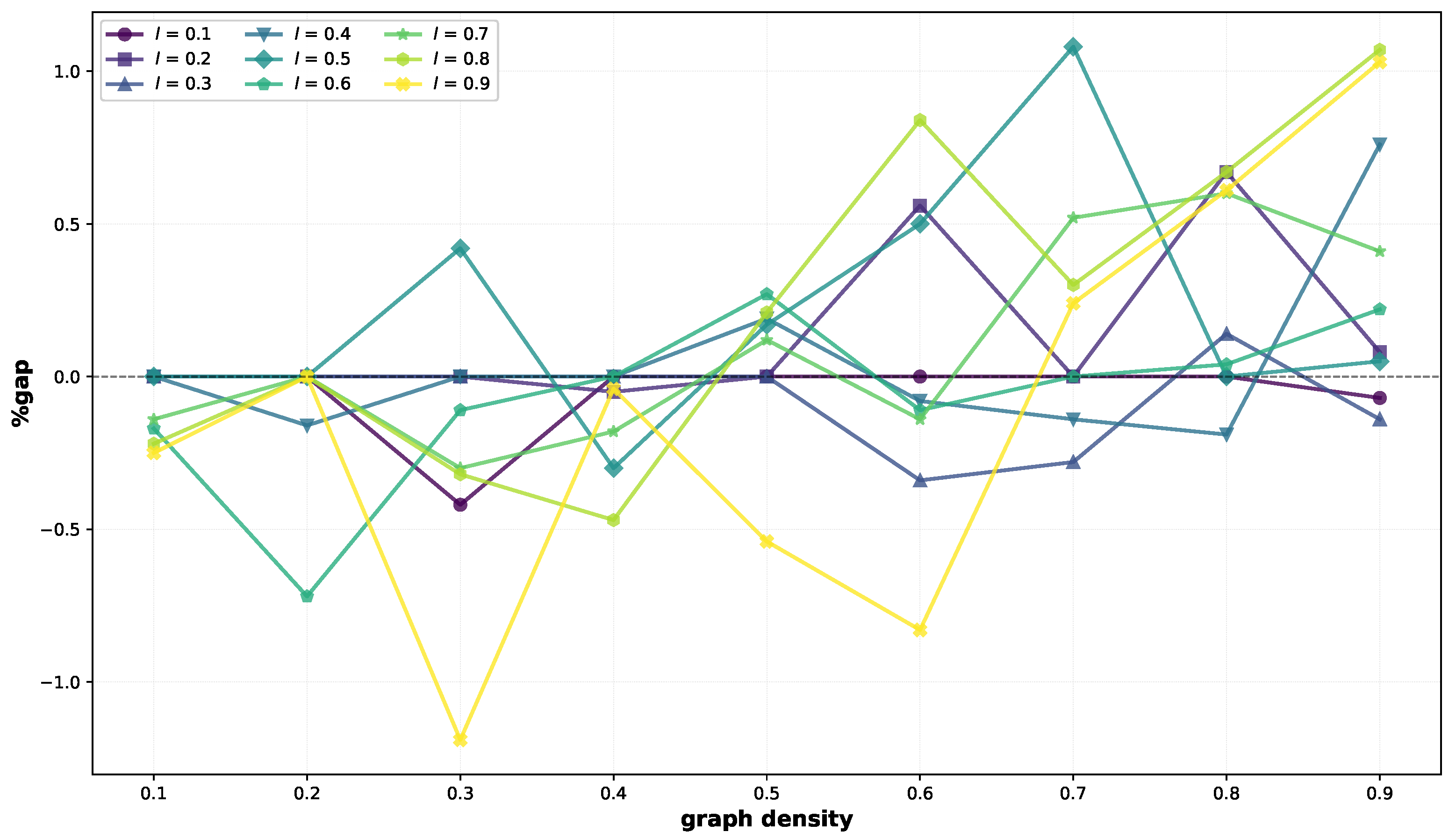
On small instances (Table 1), the two heuristics perform very similarly. Indeed, they return the same solutions (VNS gap = 0) in 26 cases out of 81, BRKGA-MFML finds better solutions on average in 28 cases (negative value in the VNS gap column), and VNS finds better solutions in the remaining 27. Gaps are very small, varying between −1.19% and 1.08%. Average computational times remain within about $1s$ for all instances with a density up to $d=0.5$, reaching $4.46s$ on average for the instances with more edges and labels ($d=l=0.9$). The comparison between BRKGA-MFML and VNS on small graphs is illustrated visually in Figure 1, where it can be seen that for most graph and label densities, gaps are close to 0, with peaks around 1% and −1%.

In accordance with the computational times, the number of generations needed to reach the best solution by BRKGA-MFML increases with d and l. In particular, it was always found in the initial population for $d=0.1$ and $l=0.1$. The average number of generations to reach this solution remains always below 2 for $d=0.1$ and up to 1.20 for $l=0.5$, and for $l=0.1$, up to 1.87 for $d=0.9$. The best solution is found after more than 10 generations on average only for $d=0.9,l\ge 0.7$, up to 11.90 generations.

Comparing with the CPLEX solutions, we can see that their values are very close. The CPLEX gap is 0 in 37 out of 81 cases and below 1% in 70 cases, increasing only twice over 2%, up to 2.63% ($d=l=0.8$).

To conclude, both heuristics prove to be very suitable for solving small instances, providing accurate solutions within fast computational times.

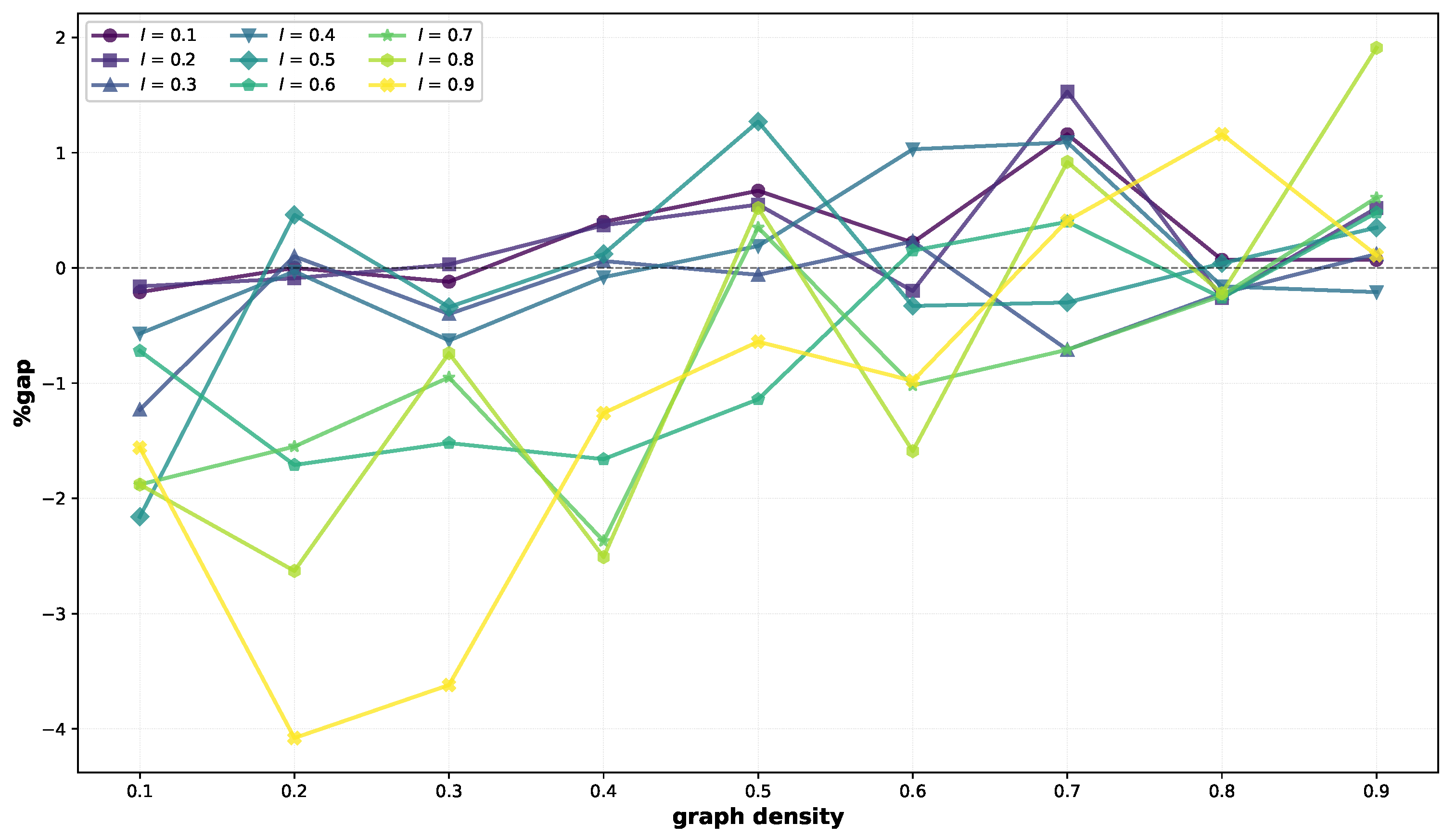
Let us now consider medium-sized instances (Table 2). Compared to the small ones, there is a more pronounced difference in performance between BRKGA-MFML and VNS. Indeed, BRKGA-MFML finds better solutions in 46 out of 81 cases, with a maximum negative gap of −4.08% ($d=0.2,l=0.9$). VNS finds better solutions in 34 cases, with a maximum gap equal to 1.91%. The 46 negative gaps average −1%, while the positive gaps average 0.52%. We can see that BRKGA-MFML is particularly effective on the less dense scenarios, finding better solutions in 23 out of 27 scenarios for $d\le 0.3$, and in 36 out of 54 scenarios for $d\le 0.6$. While the performances of the two methods appeared comparable on small graphs, on the medium ones, we can see that the diverse solutions across the search space maintained in the population by BRKGA-MFML is often beneficial for escaping from local minima. These results are illustrated in Figure 2, which shows that most gaps are negative, particularly for low graph densities and high graph densities. Similar trends will be observed for large graphs.

In terms of computational times, the heuristics run within 2 s on average for $d\le 0.3$, within 10 s for $d\le 0.6$, and within 30 s for $d\le 0.8$. On the denser instances with more labels ($d=l=0.9$), the average computational time reaches 40.70 s.

The average number of generations needed by BRKGA-MFML to find the best solution is below 2 in all cases except one for $d=0.1$, where it grows to 2.63 ($d=0.1,l=0.8$). It remains within 5 generations for $d\le 0.3$, and within 15 generations for $d\le 0.7$, increasing to over 20 generations only for $d=0.9,l\ge 0.6$ (with a maximum of 25.47 for $d=0.9$, $l=0.9$).

Comparing with CPLEX solutions, we observe that the gap is 0 in 8 cases, within 1% in 43 cases, and within 2% in 61 out of 81 cases, exceeding 4% only in 3 cases (up to 4.51% for $d=0.8,l=0.9$).

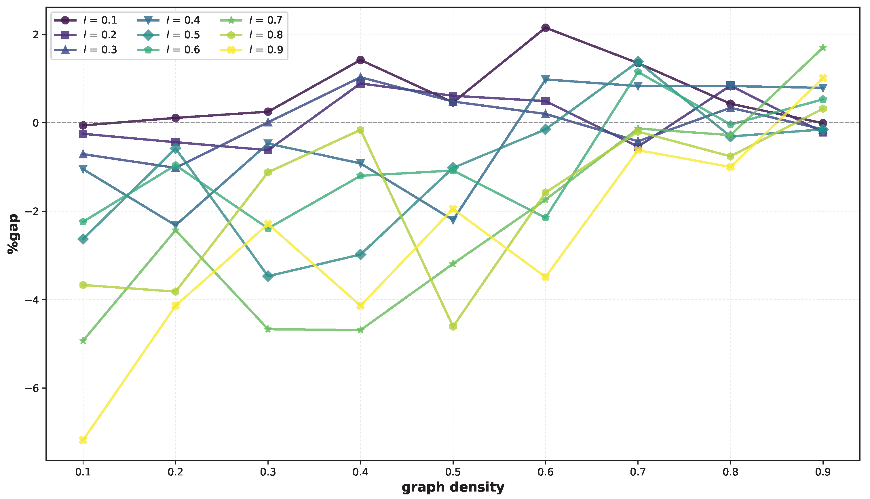
Finally, we consider the large instances. The results are reported in Table 3. For these instances, BRKGA-MFML performs better on average in 55 out of 81 cases, while VNS performs better in 26 cases. Negative gaps reach −7.18% ($d=0.1,l=0.9$). Positive gaps reach 2.15% ($d=0.6,l=0.1$); however, they are higher than 2% only once. Again, we observe that BRKGA-MFML performs particularly well for low densities, finding better solutions in 24 out of 27 cases for $d\le 0.3$ and 41 out of 54 cases for $d\le 0.7$. These trends, similar to those noted for medium graphs, are shown in Figure 3.

While higher than those observed for the other instances, computational times remain reasonable. The heuristics run within about 6 s for $d\le 0.3$, and within 60 s for $d\le 0.7$. For $d=0.7,0.8$, and $0.9$, average computational times reach around 100 s, 170 s, and 250 s, respectively. As observed for the previous cases, computational times increase according to both the d and l parameters.

The best solution is found by BRKGA-MFML on average within 4.77 generations for $d=0.1$, 5.20 generations for $d=0.2$, and 8.40 generations for $d=0.3$. The average number of generations needed exceeds 10 for $d\ge 0.5$ and $l\ge 0.5$, 20 for $d\ge 0.6$ and $l\ge 0.7$, and 30 for $d=0.9$ and $l\ge 0.7$, reaching 38.57 for $d=0.9$ and $l=0.9$.

Finally, looking at CPLEX gaps, we can see that they reach 4.81% in the worst case. However, they remain below 3% in 64 out of 81 cases.

6. Conclusions

In this work, we adapted the Biased Random-Key Genetic Algorithm paradigm to solve the Maximum Flow with Minimum Number of Labels problem (MF-ML), a challenging variant of the classical Maximum Flow problem. A key component is the definition of an appropriate decoder function that assigns a feasible solution of the problem to each chromosome in the population. The computational results, determined for a wide range of instances, show that the proposed approach outperformed a previously proposed Skewed Variable Neighborhood Search metaheuristic (VNS). In particular, when considering the largest tested graphs, with a size between 80 and 100 nodes, BRKGA-MFML outperformed VNS in 55 out of 81 scenarios, with an average improvement per scenario reaching 7.18%.

In the future, we intend to develop effective exact approaches for MF-ML and derive new theoretical insights to further improve the proposed heuristic method.

References

1. Granata, D. On penalized reload cost path, walk, tour and maximum flow: Hardness and approximation. Optim. Lett. 2025, 19, 123–138. [Google Scholar] [CrossRef]
2. Cerrone, C.; Cerulli, R.; Golden, B. Carousel greedy: A generalized greedy algorithm with applications in optimization. Comput. Oper. Res. 2017, 85, 97–112. [Google Scholar] [CrossRef]
3. Chang, R.-S.; Leu, S.-J. The minimum labeling spanning trees. Inf. Process. Lett. 1997, 63, 277–282. [Google Scholar] [CrossRef]
4. Brüggemann, T.; Monnot, J.; Woeginger, G.J. Local search for the minimum label spanning tree problem with bounded color classes. Oper. Res. Lett. 2003, 31, 195–201. [Google Scholar] [CrossRef]
5. Lai, X.; Cen, Y. Performance of a simple ACO on the minimum label spanning tree problem. Discov. Appl. Sci. 2025, 7, 367. [Google Scholar] [CrossRef]
6. Xiong, Y.; Golden, B.; Wasil, E. A one-parameter genetic algorithm for the minimum labeling spanning tree problem. IEEE Trans. Evol. Comput. 2005, 9, 55–60. [Google Scholar] [CrossRef]
7. da Silva, T.G.; Gueye, S.; Michelon, P.; Ochi, L.S.; Cabral, L.D.A.F. A polyhedral approach to the generalized minimum labeling spanning tree problem. EURO J. Comput. Optim. 2019, 7, 47–77. [Google Scholar] [CrossRef]
8. Cerrone, C.; D’Ambrosio, C.; Raiconi, A. Heuristics for the strong generalized minimum label spanning tree problem. Networks 2019, 74, 148–160. [Google Scholar] [CrossRef]
9. Zhang, P.; Fu, B. The label cut problem with respect to path length and label frequency. Theor. Comput. Sci. 2016, 648, 72–83. [Google Scholar] [CrossRef]
10. Faria, L.; Klein, S.; Sau, I.; Souza, U.S.; Sucupira, R. Maximum cuts in edge-colored graphs. Discret. Appl. Math. 2020, 281, 229–234. [Google Scholar] [CrossRef]
11. Granata, D.; Cerulli, R.; Scutellà, M.G.; Raiconi, A. Maximum Flow Problems and an NP-Complete Variant on Edge-Labeled Graphs. In Handbook of Combinatorial Optimization; Pardalos, P.M., Du, D.-Z., Graham, R.L., Eds.; Springer: New York, NY, USA, 2013; pp. 1913–1948. [Google Scholar] [CrossRef]
12. Coudert, D.; Pérennes, S.; Rivano, H.; Voge, M.-E. Combinatorial optimization in networks with Shared Risk Link Groups. Discret. Math. Theor. Comput. Sci. 2014, 18. [Google Scholar] [CrossRef]
13. Hassin, R.; Monnot, J.; Segev, D. Approximation algorithms and hardness results for labeled connectivity problems. J. Comb. Optim. 2007, 14, 437–453. [Google Scholar] [CrossRef]
14. Yuan, S.; Varma, S.; Jue, J.P. Minimum-color path problems for reliability in mesh networks. In Proceedings of the IEEE 24th Annual Joint Conference of the IEEE Computer and Communications Societies, Miami, FL, USA, 13–17 March 2005; Volume 4, pp. 2658–2669. [Google Scholar] [CrossRef]
15. Silberholz, J.; Raiconi, A.; Cerulli, R.; Gentili, M.; Golden, B.; Chen, S. Comparison of heuristics for the colourful travelling salesman problem. Int. J. Metaheuristics 2013, 2, 141–173. [Google Scholar] [CrossRef]
16. Cerulli, R.; Dell’Olmo, P.; Gentili, M.; Raiconi, A. Heuristic approaches for the Minimum Labelling Hamiltonian Cycle Problem. Electron. Notes Discret. Math. 2006, 25, 131–138. [Google Scholar] [CrossRef]
17. Couëtoux, B.; Gourvès, L.; Monnot, J.; Telelis, O.A. Labeled Traveling Salesman Problems: Complexity and approximation. Discret. Optim. 2010, 7, 74–85. [Google Scholar] [CrossRef]
18. Wu, B.Y. On the maximum disjoint paths problem on edge-colored graphs. Discret. Optim. 2012, 9, 50–57. [Google Scholar] [CrossRef]
19. Gonçalves, J.F.; Resende, M.G.C. Biased random-key genetic algorithms for combinatorial optimization. J. Heuristics 2011, 17, 487–525. [Google Scholar] [CrossRef]
20. De Freitas, C.C.; Aloise, D.J.; Da Costa Fontes, F.F.; Santos, A.C.; Da Silva Menezes, M. A biased random-key genetic algorithm for the two-level hub location routing problem with directed tours. OR Spectr. 2023, 45, 903–924. [Google Scholar] [CrossRef]
21. Carrabs, F. A biased random-key genetic algorithm for the set orienteering problem. Eur. J. Oper. Res. 2021, 292, 830–854. [Google Scholar] [CrossRef]
22. Homayouni, S.M.; Fontes, D.B.M.M.; Gonçalves, J.F. A multistart biased random key genetic algorithm for the flexible job shop scheduling problem with transportation. Int. Trans. Oper. Res. 2023, 30, 688–716. [Google Scholar] [CrossRef]
23. Gonçalves, J.F.; Resende, M.G.C.; Toso, R.F. An experimental comparison of biased and unbiased random-key genetic algorithms. Pesqui. Oper. 2014, 34, 143–164. [Google Scholar] [CrossRef]
24. Cerulli, R.; D’Ambrosio, C.; Raiconi, A. A biased random-key genetic algorithm for the knapsack problem with forfeit sets. Soft Comput. 2024, 28, 12021–12041. [Google Scholar] [CrossRef]
25. Wolpert, D.H.; Macready, W.G. No free lunch theorems for optimization. IEEE Trans. Evol. Comput. 1997, 1, 67–82. [Google Scholar] [CrossRef]
26. Gonçalves, J.F.; Resende, M.G.C.; Mendes, J.J. A biased random-key genetic algorithm with forward-backward improvement for the resource constrained project scheduling problem. J. Heuristics 2011, 17, 467–486. [Google Scholar] [CrossRef]
27. Toso, R.F.; Resende, M.G.C. A C++ application programming interface for biased random-key genetic algorithms. Optim. Methods Softw. 2015, 30, 81–93. [Google Scholar] [CrossRef]
Figure 1. BRKGA-MFML vs. VNS solution comparison on small graphs.
Mathematics 13 03621 g001
Figure 2. BRKGA-MFML vs. VNS solution comparison on medium graphs.
Mathematics 13 03621 g002
Figure 3. BRKGA-MFML vs. VNS solution comparison on large graphs.
Mathematics 13 03621 g003