Article

Fractional Modeling and Dynamic Analysis of COVID-19 Transmission with Computational Simulations

by
Mohamed. M. Alarady
,
Mohamed A. Barakat
* and
Mohamed M. Darwish
Department of Computer Science, University College of Alwajh, University of Tabuk, Al Wajh 48721, Saudi Arabia
*
Author to whom correspondence should be addressed.
Mathematics 2025, 13(22), 3619; https://doi.org/10.3390/math13223619
Submission received: 11 October 2025 / Revised: 5 November 2025 / Accepted: 7 November 2025 / Published: 12 November 2025
(This article belongs to the Section C: Mathematical Analysis)

Abstract

Most existing fractional models of COVID-19 describe only the infection process without explicitly accounting for the role of vaccination. In this study, a refined Caputo fractional model is proposed that incorporates a vaccinated class to better understand how immunization influences disease progression. The mathematical formulation guarantees the existence, uniqueness, and positivity of solutions, ensuring that all system trajectories remain biologically valid. The equilibrium points are obtained, and the reproduction number is derived to identify the conditions for disease control. The stability investigation covers local behavior alongside Ulam–Hyers and its extended variants, ensuring the system remains stable under small perturbations. Numerical experiments performed with the Adams–Bashforth–Moulton algorithm illustrate that vaccination reduces infection peaks and shortens the epidemic duration. Overall, the proposed framework enriches fractional epidemiological modeling by providing deeper insight into the combined effects of memory and vaccination in controlling infectious diseases.

1. Introduction

The basic concept of epidemics dates back to antiquity. Infectious diseases like malaria are described in the Ebers Papyrus, one of the oldest surviving medical writings, which dates to around 1500 BC [1]. In the twentieth century, mathematical modeling emerged as the primary method for researching disease dynamics, and academics from all over the world have been considering epidemic breakouts throughout history [2]. Building on this foundation, later advances examined the role of infection consciousness as well as the processes of transmission, supported by thorough stability investigations in [3,4,5]. Through leishmaniasis, tuberculosis, viruses, and most recently, COVID-19, disease-centric models of diseases from HIV and pine wilt were developed in subsequent years [6,7,8].
Mathematical epidemiology research was greatly accelerated by the global COVID-19 crisis, which validated the significance of modeling in understanding spread, evaluating therapies, and guiding health policy. The basis of most of this activity was established by Hethcote’s groundbreaking writings [9]. Remuzzi’s [10] analysis and other preliminary investigations emphasized the necessity for quick decisions and the enormous strain that the initial wave of the emergency placed on Italy’s healthcare system. As the pandemic progressed, models themselves started to incorporate memory effects in an attempt to represent its increased complexity. In order to demonstrate the additional realism that fractional models may provide, Baba and Nasidi [11] included fractional-order expressions, and Bhatter et al. [12] selected the Caputo–Fabrizio derivative. Further research [13,14,15] has since illustrated that fractional modeling offers a more flexible and realistic framework than classical integer-order schemes.
From 2021 onward, vaccination strategies became a central theme in COVID-19 modeling. For instance, Gozalpour et al. [16] proposed an eight-compartment model treating vaccination as an external preventive measure, while Sen [17] developed a discrete SEIR framework that integrates vaccination through a feedback control mechanism. Kumar and co-authors [18] further advanced the field by designing both integer- and fractional-order SEIR models that account for vaccination rates, whereas Sen [19] formulated a dual-control SEIR model that combines vaccination with antiviral treatment. More recent studies have placed greater emphasis on qualitative properties such as stability, boundedness, and non-negativity, as highlighted in the SEIR-type analysis of Sen [20] under vaccination and treatment interventions.
At the same time, fractional calculus has played an increasingly prominent role in capturing memory and hereditary effects in epidemic systems. Barakat et al. [21] proposed novel fractional approaches for Langevin equations, showing how generalized operators enrich dynamic modeling. Rashid and collaborators applied fractal–fractional techniques to cholera dynamics [22], and later combined Elzaki transforms with decomposition methods to obtain approximate solutions of Caputo-based models [23]. Using the fractional Fourier transform, Selvam et al. [24] investigated Ulam-type stability in fractional differential equations, providing fresh perspectives on the Caputo framework. Agarwal, Baleanu, and co-authors [25] made additional theoretical and practical developments that expanded the use of fractional analysis in modeling. Continuing this momentum, Omame et al. [26] used Banach’s fixed-point theorem to prove the well-posedness of a fractional COVID-19 model with numerous vaccination techniques, guaranteeing theoretical robustness. More recently, Al-Shbeil and colleagues [27] presented a model of COVID-19 that takes into consideration those who have received vaccinations. By conducting a thorough stability study, they demonstrated that a high enough vaccination threshold can eradicate the epidemic. In the analytical part of this study, the concept of fixed-point theory plays a crucial role in demonstrating the existence and uniqueness of solutions for the proposed fractional-order system. The adopted approach follows recent developments in applying fixed-point techniques to fractional boundary value problems and nonlinear dynamical systems. In particular, our results are conceptually related to those presented in [28,29], where iterative fixed-point frameworks and convergence analyses were successfully applied to similar classes of fractional operators. This connection emphasizes that the theoretical results derived in this paper are consistent with modern fixed-point-based methodologies and extend their applicability to epidemic-type fractional models.
The aim of this study is driven by the urgent need to develop more realistic mathematical models that can accurately describe the spread of infectious diseases such as COVID-19. Standard models often overlook the influence of previous states on current dynamics, which is a critical aspect of real-world epidemics. To address this, we adopt a fractional-order framework that naturally incorporates memory effects, offering a more accurate reflection of disease progression. The model also integrates vaccination as a key control measure, allowing for a closer examination of its effect on reducing transmission. In addition, through the examination of the stability of the model under small perturbations, we are assured of the stability of its predictions. The methodology offers a sound mathematical framework through which one can examine intervention strategies’ efficacies and enhance the understanding of epidemic dynamics. This paper is structured to provide a comprehensive study of a fractional-order COVID-19 model incorporating vaccination and memory effects. It begins with an introduction that outlines the motivation for using fractional derivatives to capture real-world disease dynamics more accurately. The model is then formulated using Caputo derivatives and includes compartments for susceptible, recovered, vacci- nated, infected, and severely infected individuals. The theoretical section establishes key mathematical properties such as the existence, uniqueness, and positivity of solutions, and the invariant region. Stability analysis is performed using local stability together with Ulam–Hyers and extended stability concepts. A numerical procedure of the Adams–Bashforth–Moulton algorithm is adopted to approximate solutions, while the simulation results are provided in support of the findings, which illustrate the impacts of the fractional order of infection spreading. This manuscript is finalized with discussions of the success of fractional modeling in simulating long-term disease dynamics and contributing to public health interventions.

2. Preliminaries

Definition 1
([30]). Assume σ > 0 and let f be an element of L 1 ( [ 0 , b ] , R ) , where [ 0 , b ] R + . The Riemann–Liouville fractional integral of order σ applied to f is defined by
J σ f ( t ) = 1 Γ ( σ ) 0 t ( t τ ) σ 1 f ( τ ) d τ , t > 0 ,
where Γ ( · ) is the gamma function, given by
Γ ( σ ) = 0 τ σ 1 e τ d τ .
Definition 2
([30]). Let m N be such that m 1 < σ < m , and assume f C m [ 0 , b ] . The Caputo fractional derivative of order σ for f is given by
D σ c f ( t ) = 1 Γ ( m σ ) 0 t ( t τ ) m σ 1 f ( m ) ( τ ) d τ , t > 0 .
Lemma 1
([30]). If Re ( σ ) > 0 , let m = Re ( σ ) + 1 and suppose f A C m ( 0 , b ) . Then,
( J σ   D σ c f ) ( t ) = f ( t ) k = 1 m D 0 k f ( 0 + ) k ! t k .
In particular, if 0 < σ 1 , then
( J σ D σ c f ) ( t ) = f ( t ) f ( 0 ) .
Theorem 1
([31]). [Arzelà–Ascoli] If S is compact, then a subset F C ( S ) is conditionally compact if and only if it is bounded and equicontinuous.

3. Fractional COVID-19 Model with an Immunization Structure

To account more meaningfully for transmission dynamics of epidemics, the whole population ( N ) is split into three broad classes: susceptible individuals, infected individuals, and dead individuals. The large classes are further split into meaningful subclasses.
There are three compartments of the susceptible category, namely, individuals that have never been infected but are not vaccinated ( S ) , individuals that recovered from earlier infection but have the chance of becoming infected again ( R ) , and individuals that have been vaccinated ( V ) .
The infected class is split into two subsets. The first, which is given by ( I ) , includes individuals with relatively high immunity, such that infection does not pose high risks. Proportional to the total infected are individuals of this class, denoted by some fraction χ ( χ 1 ). The second class, given by ( I d ) , denotes high-risk individuals such as pregnant women, elderly people, or individuals with chronic diseases, and they account for the remaining fraction ( 1 χ ) . The final class ( D ) comprises individuals that have succumbed due to the disease. The dynamics of each class and its movement are given by the descriptions below.

3.1. Definition of State Variables and Model Parameters

For clarity, we now describe every state variable and model parameter, explaining their meaning and role in the dynamics

3.1.1. Susceptible Class ( S )

The susceptible compartment increases at a rate Ω , which corresponds to births in a closed population. Susceptible individuals acquire infection at a rate ρ 1 ( I + I d ) , where
ρ 1 = p 1 μ N ,
with μ denoting the average number of contacts per individual per unit time, p 1 the transmission probability, and N the total population size. In addition, individuals may exit this class through vaccination at rate β or through natural death at rate γ .

3.1.2. Recovered Class ( R )

This class contains individuals who have recovered from infection ( I or I d ) at rate ε . Members of this group may be reinfected at a rate ρ 2 ( I + I d ) , where
ρ 2 = p 2 μ N , ρ 2 < ρ 1 .
As in the susceptible class, recovered individuals may leave through vaccination at rate β or natural mortality at rate γ .

3.1.3. Vaccinated Class ( V )

The vaccinated compartment consists of individuals originating either from S or R who have received the vaccine. Vaccination occurs at rate β , and while these individuals are not completely immune, their risk of infection is substantially lower. Members of this class may still contract the infection at rate ρ 3 ( I + I d ) , where
ρ 3 = p 3 μ N , ρ 3 < ρ 2 < ρ 1 ,
due to reduced transmission probability p 3 . Natural mortality also occurs in this group at rate γ .

3.1.4. Mild Infection Class ( I )

This class is composed of individuals who become infected from S , R , or V at a combined rate
χ ( ρ 1 + ρ 2 ) + ρ 3 ( I + I d ) .
They leave this class through recovery at rate ε or natural death at rate γ . No epidemic-related mortality is assumed in this subgroup.

3.1.5. Severe Infection Class ( I d )

This compartment represents individuals who acquire infection from S and R but excludes those from V , as vaccination provides protection against severe outcomes. The entry rate is given by
( 1 χ ) ( ρ 1 + ρ 2 ) ( I + I d ) .
Individuals exit the class through recovery at rate ε , natural death at rate γ , or disease-induced mortality at rate δ .

3.1.6. Death Class ( D )

The death class includes individuals who die from the epidemic at rate δ .
Building on these classifications, Al-Shbeil et al. [27] formulated a mathematical framework to describe the transitions rigorously, as presented in the following system.
d S d t = Θ ρ 1 I + I d S β + γ S , d R d t = ε I + ε I d ρ 2 I + I d R β + γ R , d V d t = β S + β R ρ 3 I + I d V γ V , d I d t = χ ρ 1 I + I d S + ρ 2 I + I d R + ρ 3 I + I d V ε I γ I , d I d d t = 1 χ ρ 1 I + I d S + ρ 2 I + I d R ε I d γ I d δ I d .
With the nonnegative initial conditions
S ( 0 ) , R ( 0 ) , V ( 0 ) , I ( 0 ) , I d ( 0 ) 0 ,
the total population is as follows:
N ( t ) = S ( t ) + R ( t ) + V ( t ) + I ( t ) + I d ( t ) .
The construction of the model is based on two main assumptions. First, the emergence of new infections is taken to be directly proportional to the transmission parameters ρ 1 , ρ 2 , and ρ 3 . Second, the incidence of infection decreases as the recovery rate ε and the vaccination rate β increase, reflecting the mitigating impact of treatment and immunization.

3.2. A Fractional Approach Utilizing the Caputo Operator

Drawing on these insights, our current research transitions to a fractional-order framework, aiming to capture long-term dependencies and memory effects more accurately, thus offering a richer perspective on real-world epidemic dynamics.
D σ c S ( t ) = Θ ρ 1 I + I d S β + γ S , D σ c R ( t ) = ε ( I + I d ) ρ 2 I + I d R β + γ R , D σ c V ( t ) = β S + β R ρ 3 I + I d V γ V , D σ c I ( t ) = χ ρ 1 I + I d S + ρ 2 I + I d R + ρ 3 I + I d V ε I γ I , D σ c I d ( t ) = 1 χ ρ 1 I + I d S + ρ 2 I + I d R ε I d γ I d δ I d .
The Caputo formulation in (12) explicitly incorporates memory effects via the fractional order σ , in contrast to the traditional integer-order baseline (11).
A full list of the model variables and parameters used in the fractional model (12) is given in Table 1.

4. Qualitative Analysis of a Fractional COVID-19 Model

In this section, we examine a fractional-order model of COVID-19 that tracks the dynamics of five distinct groups: those who are susceptible, those who have recovered, those who have been vaccinated, and individuals with either mild or severe infections. The formulation employs the Caputo fractional derivative, as follows:
D σ c H ( t ) = Ω ( t , H ( t ) ) , t [ 0 , T ] , H ( 0 ) = H 0 ,
where
H ( t ) = S ( t ) R ( t ) V ( t ) I ( t ) I d ( t ) , H 0 = S 0 R 0 V 0 I 0 I d , 0 ,
and the nonlinear function
Ω ( t , H ( t ) ) = Ω 1 ( t , H ( t ) ) Ω 2 ( t , H ( t ) ) Ω 3 ( t , H ( t ) ) Ω 4 ( t , H ( t ) ) Ω 5 ( t , H ( t ) )
encapsulates the dynamics of each compartment.
Define the Banach space
X = C [ 0 , T ] , R ,
with the norm
H = max t [ 0 , T ] | S ( t ) | + | R ( t ) | + | V ( t ) | + | I ( t ) | + | I d ( t ) | .
The following integral form is mathematically identical to the model given in (13).
H ( t ) = H 0 + 1 Γ ( σ ) 0 t ( t s ) σ 1 Ω ( s , H ( s ) ) d s .
We set forth the following assumptions to facilitate the analysis of the Covid-19 model (13):
( C 1 )
There is a constant Ω > 0 verifying:
Ω ( t , H 1 ( t ) ) Ω ( t , H 2 ( t ) ) Ω H 1 ( t ) H 2 ( t ) .
( C 2 )
Consider a nonnegative, nondecreasing continuous mapping K : [ 0 , ) [ 0 , ) that complies with the condition:
K ( u H ) u K ( H ) , u 1 ,
alongside a suitable function Ξ X such that
Ω ( t , H ( t ) )     Ξ ( t ) K ( | H ( t ) | ) .
( C 3 )
Let ϖ , Λ > 0 be constants chosen in accordance with the inequality:
Λ H 0 + sup π [ 0 , T ] Ξ ( π ) K ( ϖ ) T σ Γ ( σ + 1 ) > 1 .
Employing these assumptions, the existence of solutions to model is verified (13).
In what follows, we utilize the nonlinear Leray–Schauder alternative fixed-point theorem from Zeidler [32] to confirm the existence and uniqueness for the abstract Caputo system (13), using its equivalent Volterra formulation (14).
Theorem 2.
Suppose conditions ( C 2 ) and ( C 3 ) hold true for each Ω C [ 0 , T ] , R 5 . Then the Covid-19 model specified by Equation (13) possesses at least one solution defined on the interval [ 0 , ω ] .
Proof. 
Define the closed ball as follows:
[ B ] ϖ = { H X : H   ϖ } ,
and introduce the operator Q : X X explicitly by:
( QH ) ( t ) = H 0 + 1 Γ ( σ ) 0 t ( t s ) σ 1 Ω ( s , H ( s ) ) d s .
Employing conditions ( C 2 ) and ( C 3 ) , we obtain:
| ( QH ) ( ζ ) |     H 0 + 1 Γ ( σ ) 0 ζ ( ζ π ) σ 1 Ω ( π , H ( π ) ) d π         H 0 + 1 Γ ( σ ) 0 ζ ( ζ π ) σ 1 Ω ( π , H ( π ) ) d π         H 0 + sup π [ 0 , T ] Ξ ( π ) K ( H ) Γ ( σ ) 0 ζ ( ζ π ) σ 1 d π         H 0 + sup π [ 0 , T ] Ξ ( π ) K ( ϖ ) T σ Γ ( σ + 1 ) < Λ .
Accordingly, the operator Q maps bounded balls in the space X into bounded subsets.
To proceed, we now show that Q is completely continuous. For this purpose, consider an arbitrary function H X and any two points 0 ζ 1 < ζ 2 T such that:
| Q H ( ζ 2 ) Q H ( ζ 1 ) | 1 Γ ( σ ) 0 ζ 2 ( ζ 2 π ) σ 1 Ω ( π , H ( π ) ) d π 1 Γ ( σ ) 0 ζ 1 ( ζ 1 π ) σ 1 Ω ( π , H ( π ) ) d π 1 Γ ( σ ) [ 0 ζ 1 ( ζ 2 π ) σ 1 ( ζ 1 π ) σ 1 Ω ( π , H ( π ) ) d π + ζ 1 ζ 2 ( ζ 2 π ) σ 1 Ω ( π , H ( π ) ) d π ] sup ζ [ 0 , T ] Ξ ( ζ ) K ( ϖ ) Γ ( σ ) 0 ζ 1 ( ζ 2 π ) σ 1 ( ζ 1 π ) σ 1 d π + sup ζ [ 0 , T ] Ξ ( ζ ) K ( ϖ ) Γ ( σ + 1 ) ( ζ 2 ζ 1 ) σ 0 as ζ 2 ζ 1 .
By the Arzelà–Ascoli theorem, Q is a compact (completely continuous) operator.
It remains to show that any H X satisfying
H = d Q H for some d ( 0 , 1 )
must lie in a bounded subset of X . Indeed, if H solves this equation, then for each ζ ( 0 , T ) we obtain:
| H ( ζ ) | = d | ( Q H ) ( ζ ) | H 0 + sup ζ [ 0 , T ] Ξ ( ζ ) K ( | H ( ϖ ) | ) Γ ( σ + 1 ) T σ .
Hence,
H H 0 + sup ζ [ 0 , T ] Ξ ( ζ ) K ( | H ( ϖ ) | ) Γ ( σ + 1 ) T σ .
Referring to assumption ( C 3 ) , it follows that H Λ . Define the open ball:
B Λ : = H X : H   <   Λ .
It follows that the operator Q : B Λ X is completely continuous. Additionally, no function H B Λ satisfies the equation H = d Q H . Therefore, applying the nonlinear Leray–Schauder fixed-point theorem, we conclude that the model (13) admits at least one solution on the interval [ 0 , T ] . □
We now proceed to establish the conditions under which the Covid-19 model (12) admits a unique solution, using the Banach contraction principle.
Theorem 3.
Assume that the function Ω : [ 0 , T ] × X R 5 is continuous and satisfies the Lipschitz condition ( C 1 ) for any pair H 1 , H 2 X . Then, the model (12) admits a unique solution on the interval [ 0 , T ] , provided the inequality
Ω T σ < Γ ( σ + 1 )
holds.
Proof. 
Assume that H [ B ] h , where the parameter h is chosen to satisfy the inequality:
h Γ ( σ + 1 ) H 0 + Y T σ Γ ( σ + 1 ) Ω T σ ,
with Y : = sup ζ [ 0 , T ] Ω ( ζ , 0 ) .
We now estimate the operator Q applied to H :
| Q H ( ζ ) | H 0 + 1 Γ ( σ ) 0 ζ ( ζ π ) σ 1 Ω ( π , H ( π ) ) d π H 0 + 1 Γ ( σ ) 0 ζ ( ζ π ) σ 1 Ω ( π , H ( π ) ) Ω ( π , 0 ) + Ω ( π , 0 ) d π H 0 + h Ω + Y Γ ( σ ) 0 ζ ( ζ π ) σ 1 d π H 0 + ( h Ω + Y ) T σ Γ ( σ + 1 ) h .
This shows that the operator Q maps the ball [ B ] h into itself. That is,
Q ( [ B ] h ) [ B ] h .
Now, let us consider two functions H 1 , H 2 [ B ] h and fix any ζ [ 0 , T ] . We examine the difference between their images under the operator Q :
( Q H 1 ) ( ζ ) ( Q H 2 ) ( ζ ) 1 Γ ( σ ) 0 ζ ( ζ π ) σ 1 Ω ( π , H 1 ( π ) ) Ω ( π , H 2 ( π ) ) d π .
Since Ω satisfies a Lipschitz condition with constant Ω , we can estimate:
( Q H 1 ) ( ζ ) ( Q H 2 ) ( ζ ) Ω Γ ( σ ) 0 ζ ( ζ π ) σ 1 H 1 ( π ) H 2 ( π ) d π Ω T σ Γ ( σ + 1 ) H 1 H 2 .
Since Ω T σ Γ ( σ + 1 ) < 1 by assumption, the operator Q is a contraction. Therefore, by the Banach fixed-point theorem, there exists a unique function H [ B ] h such that
Q H = H .
This fixed point corresponds to a solution of the integral equation and thus to the original model (13).
To confirm uniqueness, assume there are two solutions H 1 and H 2 such that Q H 1 = H 1 and Q H 2 = H 2 . Then,
H 1 H 2 = Q H 1 Q H 2 < H 1 H 2 ,
which is a contradiction unless H 1 = H 2 . Hence, the solution must be unique. We conclude that the fractional model (12) admits a unique solution in the space X . □
Before analyzing the long-term behavior of the model, it is essential to verify that the system’s solutions remain within biologically reasonable bounds. In particular, we aim to confirm that the total population governed by the model does not grow without limit. This is addressed by identifying a set in the state space that traps the trajectories of the system. The result below demonstrates that this region is invariant under the dynamics.
Theorem 4.
Let the fractional-order system (12) be governed by Caputo derivatives of order σ ( 0 , 1 ) . Then, the set
R = ( S , R , V , I , I d ) R + 5 | S + R + V + I + I d Θ γ
is positively invariant.
Proof. 
Define the total population as follows:
N ( ζ ) = S ( ζ ) + R ( ζ ) + V ( ζ ) + I ( ζ ) + I d ( ζ ) .
By adding the fractional equations in the system, we obtain:
D ζ σ C S ( ζ ) + D ζ σ C R ( ζ ) + D ζ σ C V ( ζ ) + D ζ σ C I ( ζ ) + D ζ σ C I d ( ζ ) = Θ γ N ( ζ ) ρ 3 ( 1 χ ) ( I ( ζ ) + I d ( ζ ) ) V ( ζ ) δ I d ( ζ ) ,
which implies
D σ c N ( ζ ) = = Θ γ N ( ζ ) ρ 3 ( 1 χ ) ( I ( ζ ) + I d ( ζ ) ) V ( ζ ) δ I d ( ζ ) Θ γ N ( ζ ) .
From the initial data, we have:
N ( 0 ) = S ( 0 ) + R ( 0 ) + V ( 0 ) + I ( 0 ) + I d ( 0 ) .
Now consider the auxiliary problem:
D ζ σ C u ( ζ ) = Θ γ u ( ζ ) , u ( 0 ) = N ( 0 ) .
The exact solution is known to be:
u ( ζ ) = Θ γ Θ γ N ( 0 ) E σ ( γ ζ σ ) ,
where E σ ( · ) is the Mittag-Leffler function. Since E σ ( γ ζ σ ) ( 0 , 1 ) for γ , ζ > 0 , we conclude:
u ( ζ ) Θ γ , for all ζ 0 .
Applying the comparison principle for Caputo fractional derivatives, we get:
N ( ζ ) u ( ζ ) Θ γ , for all ζ 0 .
Thus,
0 N ( ζ ) Θ γ ,
Hence, for any initial condition ( S ( 0 ) , R ( 0 ) , V ( 0 ) , I ( 0 ) , I d ( 0 ) ) R , the total population satisfies 0 N ( ζ ) Θ / γ for all ζ 0 . This confirms that the set R is invariant under the system dynamics, meaning that all trajectories starting inside R remain bounded and never leave this region throughout the evolution of the model. invariant. □

5. Fixed Points and Basic Reproduction Number

To determine the steady states of the proposed Caputo fractional model (12), all fractional derivatives are set equal to zero.

5.1. Disease-Free Equilibrium (DFE)

When infection is absent, i.e., I = I d = 0 , the model reduces to
R * = 0 , S * = Θ β + γ , V * = β Θ γ ( β + γ ) , I * = I d * = 0 .
Thus, the total population at equilibrium satisfies
N * = S * + V * = Θ γ ,
which agrees with the invariant population bound.

5.2. Endemic Equilibrium (EE)

If infection persists ( I + I d > 0 ), let Y = I + I d . At equilibrium, the model yields
S = Θ β + γ + ρ 1 Y , R = ε Y β + γ + ρ 2 Y , V = β ( S + R ) γ + ρ 3 Y .
For the infected compartments, we have
0 = χ [ ρ 1 S + ρ 2 R + ρ 3 V ] Y ( ε + γ ) I , 0 = ( 1 χ ) [ ρ 1 S + ρ 2 R ] Y ( ε + γ + δ ) I d ,
where Y = I + I d . These equations specify the endemic equilibrium.

5.3. Basic Reproduction Number

To determine the basic reproduction number R 0 associated with the proposed Caputo fractional COVID–19 model, we employ the next-generation matrix approach, which is based on the linearization of the infected subsystem around the disease-free equilibrium (DFE). Although the system involves a fractional derivative, the steady state and the reproduction number are derived in the same way as in the classical case, since the fractional order σ influences only the rate of convergence and not the equilibrium itself.
The infectious dynamics of the model are governed by the following equations:
D t σ c I = χ [ ρ 1 S + ρ 2 R + ρ 3 V ] ( I + I d ) ( ε + γ ) I , D t σ c I d = ( 1 χ ) [ ρ 1 S + ρ 2 R ] ( I + I d ) ( ε + γ + δ ) I d ,
where I and I d denote, respectively, the undetected and detected infectious populations. The first terms on the right-hand sides correspond to the emergence of new infections, while the remaining terms represent recovery, removal, or transition to other classes.
At the DFE, all infection-related compartments vanish, while susceptible and vaccinated individuals remain at constant levels:
S * = Θ β + γ , V * = β Θ γ ( β + γ ) .
Evaluating the Jacobians of the new infection and transition terms with respect to ( I , I d ) at the DFE gives
F = χ ( ρ 1 S * + ρ 3 V * ) χ ( ρ 1 S * + ρ 3 V * ) ( 1 χ ) ρ 1 S * ( 1 χ ) ρ 1 S * , V = ε + γ 0 0 ε + γ + δ .
The next-generation matrix is defined as K = F V 1 , whose spectral radius corresponds to the basic reproduction number R 0 . After simplification, we obtain
R 0 = χ ( ρ 1 S * + ρ 3 V * ) ε + γ + ( 1 χ ) ρ 1 S * ε + γ + δ .
Substituting the equilibrium values S * and V * into the expression yields
R 0 = Θ β + γ χ ρ 1 + ρ 3 β γ ε + γ + ( 1 χ ) ρ 1 ε + γ + δ .
The parameter R 0 represents the expected number of secondary infections produced by one infectious individual introduced into a completely susceptible population.

6. Stability Insights

6.1. Stability Analysis Near the Disease-Free Equilibrium

Theorem 5.
Let  E 0 = S * , R * , V * , I * , I d * = Θ β + γ , 0 , β Θ γ ( β + γ ) , 0 , 0  be the disease–free equilibrium (DFE) of (12). If  R 0 < 1 , then  E 0  is locally asymptotically stable.
Proof. 
Consider the state vector x = ( S , R , V , I , I d ) and the DFE
E 0 = S * , R * , V * , I * , I d * = Θ β + γ , 0 , β Θ γ ( β + γ ) , 0 , 0 .
The Caputo operator does not alter the linearization matrix; hence the Jacobian J ( E 0 ) equals the Jacobian of the right–hand side:
J ( E 0 ) = ( β + γ ) 0 0 ρ 1 S * ρ 1 S * 0 ( β + γ ) 0 ε ε β β γ ρ 3 V * ρ 3 V * 0 0 0 χ ( ρ 1 S * + ρ 3 V * ) ( ε + γ ) χ ( ρ 1 S * + ρ 3 V * ) 0 0 0 ( 1 χ ) ρ 1 S * ( 1 χ ) ρ 1 S * ( ε + γ + δ ) .
Then, the characteristic polynomial factors is
W J ( λ ) = ( λ + β + γ ) 2 ( λ + γ ) ( S , R , V ) block · λ 2 τ λ + Δ ( I , I d ) block .
Introduce the DFE combinations
B : = ρ 1 S * + ρ 3 V * , C : = ρ 1 S * ,
so that the infected block is
A = χ B ( ε + γ ) χ B ( 1 χ ) C ( 1 χ ) C ( ε + γ + δ ) .
From Equations (16) and (17), we get
τ = tr ( A ) = χ B + ( 1 χ ) C ( 2 ε + 2 γ + δ ) ,
Δ = det ( A ) = ( ε + γ ) ( ε + γ + δ ) 1 R 0 ,
From the ( S , R , V ) block we obtain three real eigenvalues
λ 1 = λ 2 = ( β + γ ) , λ 3 = γ ,
which are strictly negative. The remaining two eigenvalues, say λ 4 , λ 5 , are roots of
λ 2 τ λ + ( ε + γ ) ( ε + γ + δ ) ( 1 R 0 ) = 0 .
When R 0 < 1 , the constant term is positive; together with tr ( A ) < 0 , both roots have negative real parts. Therefore, all five eigenvalues of J ( E 0 ) lie in the open left half–plane.
For the Caputo fractional system D t σ c z = J ( E 0 ) z with 0 < σ 1 , asymptotic stability requires that every eigenvalue λ of J ( E 0 ) satisfies | arg ( λ ) | > σ π / 2 . The first three eigenvalues are λ 1 = λ 2 = ( β + γ ) and λ 3 = γ . Hence,
| arg ( λ k ) |   = π > σ π 2 , k = 1 , 2 , 3 ,
so, the stability condition is satisfied for these modes.
For the infected block, when R 0 < 1 , the constant term is positive and τ < 0 , ensuring that both roots of the quadratic have negative real parts.
If the eigenvalues are real, then λ 4 , λ 5 < 0 , giving | arg ( λ 4 , 5 ) | = π > σ π / 2 . If they are complex conjugates, λ 4 , 5 = α ± i β with α < 0 , their arguments satisfy | arg ( λ 4 , 5 ) | = arctan ( | β / α | ) , where | β / α | > 0 , implying | arg ( λ 4 , 5 ) | > π / 2 > σ π / 2 for 0 < σ 1 .
Hence, in all cases, every eigenvalue of J ( E 0 ) satisfies | arg ( λ ) | > σ π / 2 . Therefore, the disease–free equilibrium is locally asymptotically stable whenever R 0 < 1 . □

6.2. Stability of Ulam–Hyers

In the context of the proposed COVID-19 model provided by a system of Caputo-type fractional differential equations, the stability of the Ulam–Hyers type plays a critical role in determining the solution’s behavior through small perturbations. Indeed, this stability, among other things, ensures that if one has an approximate solution of the model equations, then one has a true neighboring solution. This property is of great application in epidemiological modeling, based on the fact that parameters and initial data are fraught with uncertainties.
Definition 3.
Ulam–Hyers stability of the fractional-order system (13) can be investigated by considering a perturbed function U ( ζ ) that satisfies the inequality
D σ c U ( ζ ) Ω ( ζ , U ( ζ ) ) ϵ ,
for some small ϵ > 0 , there exists an exact solution X ( ζ ) , such that
U ( ζ ) X ( ζ ) U ϵ , for all ζ [ 0 , T ] ,
where U > 0 is a constant that does not depend on ϵ.
Definition 4.
Extended Ulam–Hyers stability of the fractional-order system (13) can be investigated by considering a perturbed function U ( ζ ) that satisfies the following inequality
D σ c U ( ζ ) Ω ( ζ , U ( ζ ) ) ϵ Ψ ( ζ ) ,
for all small ϵ > 0 , and for some given non-negative function Ψ on [ 0 , T ] , there exists an exact solution X ( ζ ) , such that
U ( ζ ) X ( ζ ) Ψ ( ζ ) , for all ζ [ 0 , T ] .
A key lemma plays a central role in establishing both the extended and Ulam–Hyers types of stability for the system.
Lemma 2.
Let X X be a function that approximately satisfies the COVID-19 model (12). Assume that for all ζ [ 0 , T ] , there exists a perturbation function E X such that
E ( ζ ) ϵ , E = max { E 1 , E 2 , E 3 , E 4 , E 5 } .
and suppose that X satisfies the perturbed system:
D σ c X ( ζ ) = Ω ( ζ , X ( ζ ) ) + E ( ζ ) , X ( 0 ) = X 0 0 .
Then, the following estimate holds:
X ( ζ ) X 0 1 Γ ( σ ) 0 ζ ( ζ π ) σ 1 Ω ( π , X ( π ) ) d π ϵ T σ Γ ( σ + 1 ) .
Proof. 
From the assumed perturbed equation, the mild solution is given by:
X ( ζ ) = X 0 + 1 Γ ( σ ) 0 ζ ( ζ π ) σ 1 Ω ( π , X ( π ) ) d π + 1 Γ ( σ ) 0 ζ ( ζ π ) σ 1 E ( π ) d π .
Taking the norm of the deviation from the exact integral form yields:
X ( ζ ) X 0 1 Γ ( σ ) 0 ζ ( ζ π ) σ 1 Ω ( π , X ( π ) ) d π 1 Γ ( σ ) 0 ζ ( ζ π ) σ 1 E ( π ) d π ϵ T σ Γ ( σ + 1 ) .
Theorem 6.
Let X X and suppose Ω C ( [ 0 , T ] , R 5 ) . If the Lipschitz condition ( C 1 ) and inequality (15) hold, then the unique solution of problem (14) is both Ulam–Hyers and extended Ulam–Hyers stable.
Proof. 
Let U X be the exact solution of (14), and let X X be an approximate solution satisfying
E ( ζ ) ϵ ,
so that
D σ c X ( ζ ) = Ω ζ , X ( ζ ) + E ( ζ ) , X ( 0 ) = X 0 .
Its mild form is
X ( ζ ) = X 0 + 1 Γ ( σ ) 0 ζ ( ζ v ) σ 1 Ω v , X ( v ) d v + 1 Γ ( σ ) 0 ζ ( ζ v ) σ 1 E ( v ) d v .
Then,
X ( ζ ) U ( ζ ) 1 Γ ( σ ) 0 ζ ( ζ v ) σ 1 Ω ( v , X ( v ) ) Ω ( v , U ( v ) ) d v + 1 Γ ( σ ) 0 ζ ( ζ v ) σ 1 E ( v ) d v Ω Γ ( σ ) 0 ζ ( ζ v ) σ 1 X ( v ) U ( v ) d v + ϵ ζ σ Γ ( σ + 1 ) .
Hence, one obtains
X ( ζ ) U ( ζ ) ϵ T σ Γ ( σ + 1 ) Ω T σ = ϵ U .
Since U > 0 and given Ψ ( ϵ ) = ϵ U Ω satisfies Ψ ( 0 ) = 0 , this establishes both the Ulam–Hyers and the extended Ulam–Hyers stability of (14). □

7. Numerical Method and Simulations

We present a robust numerical method for approximating the solution of the fractional differential equation
D σ c H ( τ ) = Ω ( τ , H ( τ ) ) , τ [ 0 , T ] , H ( 0 ) = H 0 ,
where D σ c denotes the Caputo fractional derivative of order σ ( 0 , 1 ] .
By applying the fractional integral operator J σ c to Equation (22), the problem is reformulated into the Volterra-type integral equation
H ( τ ) = H ( 0 ) + 1 Γ ( σ ) 0 τ ( τ s ) σ 1 Ω ( s , H ( s ) ) d s , τ [ 0 , T ] .
To solve Equation (23) numerically, we employ the fractional Adams–Bashforth–Moulton predictor–corrector method [33,34], given by:
H n p = H ( 0 ) + h σ j = 1 n 1 a n j 1 σ Ω ( τ j , H j ) , H n = H ( 0 ) + h σ b ˜ n σ Ω ( τ 0 , H 0 ) + j = 1 n 1 b n j σ Ω ( τ j , H j ) + b 0 σ Ω ( τ n , H n p ) .
To enhance accuracy, multiple corrector iterations may be performed recursively as follows:
H n [ 0 ] = H ( 0 ) + h σ j = 1 n 1 a n j 1 σ Ω ( τ j , H j ) , H n [ η ] = H ( 0 ) + h σ b ˜ n σ Ω ( τ 0 , H 0 ) + j = 1 n 1 b n j σ Ω ( τ j , H j ) + b 0 σ Ω ( τ n , H n [ η 1 ] ) , η = 1 , 2 ,
The coefficients used in the scheme are defined by:
a n σ = ( ( n + 1 ) σ n σ ) Γ ( σ + 1 ) , b ˜ n σ = ( ( n 1 ) σ + 1 n σ ( n σ 1 ) ) Γ ( σ + 2 ) , b n σ = 1 Γ ( σ + 2 ) , n = 0 , ( ( n 1 ) σ + 1 2 n σ + 1 + ( n + 1 ) σ + 1 ) Γ ( σ + 2 ) , n 1 .
The initial conditions for the COVID-19 model are:
S ( 0 ) = 17300532 , R ( 0 ) = 30921318 , V ( 0 ) = 169017000 , I ( 0 ) = 616214 , I d ( 0 ) = 410809 .
The values of the parameters are:
β = 287010 , γ = 0.00066 , δ = 0.6 , ρ 1 = 4.4 × 10 11 , ρ 2 = 3.215 × 10 11 , ρ 3 = 1.4925 × 10 11 , μ = 0.0352 , α = 0.0166 , θ = 5.6259 × 10 4 .
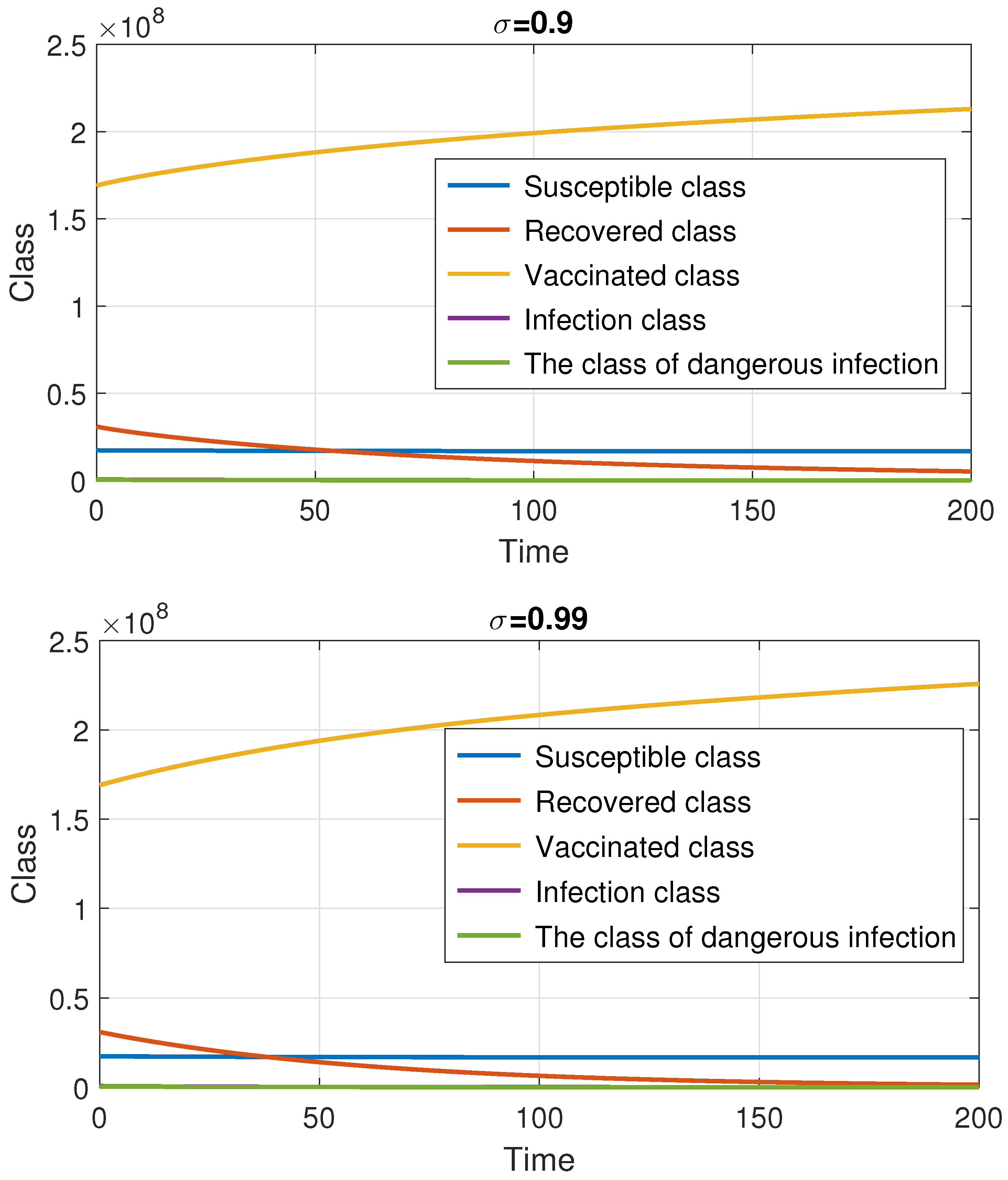
The initial conditions in (27) together with the parameters in (28) are used to simulate the model behavior. Figure 1 demonstrates the dynamics of the compartments S , R , V , I , and I d for varying values of the fractional order σ .

8. Conclusions

This paper developed a fractional model for the transmission of COVID-19 in which the Caputo operator was used to describe memory effects within the system. The model was examined analytically to confirm the existence, uniqueness, positivity, and boundedness of its solutions. The equilibrium points were identified, and the corresponding reproduction number was derived to determine the threshold for infection spread. Different forms of stability, including local, Ulam–Hyers, and generalized types, were discussed to evaluate the system’s response to small disturbances. Numerical results obtained through a fractional predictor–corrector method supported the theoretical findings and highlighted how variations in the fractional order influence the pace of infection reduction and the duration of transient behavior. This study also links fractional and classical approaches, since when σ = 1 , the model becomes the standard integer-order system known from earlier studies.
For future research, the framework may be extended to include sensitivity and optimal control analyses, parameter estimation using real epidemiological data, and comparison with other fractional operators. Such extensions would further demonstrate the adaptability of fractional modeling in capturing realistic epidemic patterns and supporting decision-making strategies. Finally, exploring alternative nonsingular fractional operators, such as Caputo–Fabrizio or Atangana–Baleanu derivatives, along with a global disease-free stability analysis, would further enrich the theoretical and practical scope of fractional epidemic models.

Author Contributions

Conceptualization, M.A.B.; methodology, M.A.B. and M.M.D.; software, M.A.B. and M.M.D.; validation, M.M.A., M.A.B. and M.M.D.; formal analysis, M.M.A., M.A.B. and M.M.D.; investigation, M.M.A., M.A.B. and M.M.D.; resources, M.M.A., M.A.B. and M.M.D.; data curation, M.A.B. and M.M.D.; writing—original draft preparation, M.M.A., M.A.B. and M.M.D.; writing—review and editing, M.M.A., M.A.B. and M.M.D.; visualization, M.M.A., M.A.B. and M.M.D.; supervision, M.A.B.; project administration, M.A.B.; funding acquisition, M.M.A., M.A.B. and M.M.D. All authors have read and agreed to the published version of the manuscript.

Funding

This research was funded by the Deanship of Research and Graduate Studies at University of Tabuk through Research No. S-0269-2024.

Data Availability Statement

The original contributions presented in this study are included in this article. Further inquiries can be directed to the corresponding authors.

Acknowledgments

The authors extend their appreciation to the Deanship of Research and Graduate Studies at University of Tabuk for funding this work through Research No. S-0269-2024.

Conflicts of Interest

The authors declare no conflict of interest.

References

  1. Thanin, S.; Anwar, Z.; Saowaluck, C.; Zohreh, E.; Mouhcine, T.; Salih, D. Analysis of a discrete mathematical COVID-19 model. Results Phys. 2021, 28, 104668. [Google Scholar] [CrossRef]
  2. Kermack, W.; McKendrick, A. Contributions to the mathematical theory of epidemics. Proc. R. Soc. A 1927, 115, 700–721. [Google Scholar]
  3. Ruan, S.; Wang, W. Dynamical behavior of an epidemic mode with a nonlinear incidence rate. J. Differ. Equ. 2003, 188, 135–163. [Google Scholar] [CrossRef]
  4. Korobeinikov, A. Global properties of infectious disease models with nonlinear incidence. Bull. Math. Biol. 2007, 69, 1871–1886. [Google Scholar] [CrossRef] [PubMed]
  5. De la Sen, M.; Alonso-Quesada, S. Vaccination strategies based on feedback control techniques for a general SEIR-epidemic model. Appl. Math. Comput. 2011, 218, 3888–3904. [Google Scholar] [CrossRef]
  6. Korobeinikov, A. Global properties of basic virus dynamics models. Bull. Math. Biol. 2004, 66, 879–883. [Google Scholar] [CrossRef] [PubMed]
  7. Souza, M.O.; Zubelli, J.P. Global stability for a class of virus models with cytotoxic T lymphocyte immune response and antigenic variation. Bull. Math. Biol. 2011, 73, 609–625. [Google Scholar] [CrossRef]
  8. Huo, H.F.; Dang, Y.S.-J.; Li, N. Stability of a two-strain tuberculosis model with general contact rate. Abstr. Appl. Anal. 2010, 2010, 293747. [Google Scholar] [CrossRef]
  9. Hethcote, H.W. Three basic epidemiological models. In Applied Mathematical Ecology; Springer: Berlin/Heidelberg, Germany, 1989; pp. 119–144. [Google Scholar]
  10. Remuzzi, A.; Remuzzi, G. COVID-19 and Italy: What next? Lancet 2020, 395, 1225–1228. [Google Scholar] [CrossRef]
  11. Baba, I.A.; Nasidi, B.A. Fractional order epidemic model for the dynamics of novel COVID-19. Alex. Eng. J. 2021, 60, 537–548. [Google Scholar] [CrossRef]
  12. Bhatter, S.; Bhatia, B.; Kumawat, S.; Purohit, S.D. Modeling and Simulation of COVID-19 Disease Dynamics via Caputo Fabrizio Fractional Derivative. Comput. Methods Differ. Equ. 2024, 13, 494–504. [Google Scholar]
  13. Kittaneh, F. Numerical radius inequalities for Hilbert space operators. Stud. Math. 2005, 168, 73–80. [Google Scholar] [CrossRef]
  14. Sababheh, M.; Moradi, H.R. More accurate numerical radius inequalities (I). Linear Multilinear Algebra 2021, 69, 1964–1973. [Google Scholar] [CrossRef]
  15. Barakat, M.A.; Saadeh, R.; Hyder, A.-A.; Qazza, A.; Aly, A.M. A Novel Fractional Model Combined with Numerical Simulation to Examine the Impact of Lockdown on COVID-19 Spread. Fractal Fract. 2024, 8, 702. [Google Scholar] [CrossRef]
  16. Gozalpour, N.; Badfar, E.; Nikoofard, A. Transmission dynamics of novel coronavirus SARS-CoV-2 among healthcare workers, a case study in Iran. Nonlinear Dyn. 2021, 105, 3749–3761. [Google Scholar] [CrossRef] [PubMed]
  17. De la Sen, M.; Alonso-Quesada, S.; Ibeas, A. On a discrete SEIR epidemic model with exposed infectivity, feedback vaccination and partial delayed re-susceptibility. Mathematics 2021, 9, 520. [Google Scholar] [CrossRef]
  18. Kumar, P.; Erturk, V.S.; Murillo-Arcila, M. A new fractional mathematical modelling of COVID-19 with the availability of vaccine. Results Phys. 2021, 24, 104213. [Google Scholar] [CrossRef]
  19. De la Sen, M.; Ibeas, A. On an SE(Is)(Ih)AR epidemic model with combined vaccination and antiviral controls for COVID-19 pandemic. Adv. Differ. Equ. 2021, 2021, 92. [Google Scholar] [CrossRef]
  20. De la Sen, M.; Ibeas, A.; Nistal, R. About partial reachability issues in an SEIR epidemic model and related infectious disease tracking in finite time under vaccination and treatment controls. Discret. Dyn. Nat. Soc. 2021, 2021, 1026–1226. [Google Scholar] [CrossRef]
  21. Barakat, M.A.; Hyder, A.A.; Rizk, D. New fractional results for Langevin equations through extensive fractional operators. AIMS Math. 2023, 8, 6119–6135. [Google Scholar] [CrossRef]
  22. Rashid, S.; Jarad, F.; Alsharidi, A.K. Numerical investigation of fractional-order cholera epidemic model with transmission dynamics via fractal–fractional operator technique. Chaos Solitons Fractals 2022, 162, 112477. [Google Scholar] [CrossRef]
  23. Rashid, S.; Kubra, K.T.; Sultana, S.; Agarwal, P.; Osman, M.S. An approximate analytical view of physical and biological models in the setting of Caputo operator via Elzaki transform decomposition method. J. Comput. Appl. Math. 2022, 413, 114378. [Google Scholar] [CrossRef]
  24. Selvam, A.; Sabarinathan, S.; Noeiaghdam, S.; Govindan, V. Fractional Fourier Transform and Ulam Stability of Fractional Differential Equation with Fractional Caputo-Type Derivative. J. Funct. Spaces 2022, 2022, 3777566. [Google Scholar] [CrossRef]
  25. Agarwal, P.; Baleanu, D.; Chen, Y.; Momani, S.; Machado, J.T. Fractional calculus. In Proceedings of the International Workshop on Advanced Theory and Applications of Fractional Calculus (ICFDA), Amman, Jordan, 16–18 July 2019. [Google Scholar]
  26. Omame, A.; Okuonghae, D.; Nwajeri, U.K.; Onyenegecha, C.P. A fractional-order multi-vaccination model for COVID-19 with non-singular kernel. Alex. Eng. J. 2022, 61, 6089–6104. [Google Scholar] [CrossRef]
  27. Al-Shbeil, I.; Djenina, N.; Jaradat, A.; Al-Husban, A.; Ouannas, A.; Grassi, G. A New COVID-19 Pandemic Model including the Compartment of Vaccinated Individuals: Global Stability of the Disease-Free Fixed Point. Mathematics 2023, 11, 576. [Google Scholar] [CrossRef]
  28. Damag, F.H. On Comparing Analytical and Numerical Solutions of Time Caputo Fractional Kawahara Equations via Some Techniques. Mathematics 2025, 13, 2995. [Google Scholar] [CrossRef]
  29. Abbas, M.; Ciobanescu, C.; Asghar, M.W.; Omame, A. Solution Approximation of Fractional Boundary Value Problems and Convergence Analysis Using AA-Iterative Scheme. AIMS Math. 2024, 9, 13129–13158. [Google Scholar] [CrossRef]
  30. Kilbas, A.; Srivastava, H.; Trujillo, J. Theory and Applications of Fractional Differential Equations; North-Holland Mathematics Studies—Elsevier: Amsterdam, The Netherlands, 2006; Volume 204. [Google Scholar]
  31. Dunford, N.; Schwartz, J. Linear Operators. Part I: General Theory; Interscience Publishers (John Wiley & Sons): New York, NY, USA, 1958; Interscience Tracts in Pure and Applied Mathematics, Volume 7. [Google Scholar]
  32. Zeidler, E. Nonlinear Functional Analysis and Its Applications: Fixed-Point Theorems; Springer: New York, NY, USA, 1986. [Google Scholar]
  33. Diethelm, K.; Ford, N.J.; Freed, A.D. Detailed error analysis for a fractional Adams method. Numer. Algorithms 2004, 36, 31–52. [Google Scholar] [CrossRef]
  34. Diethelm, K.; Ford, N.J.; Freed, A.D. A predictor-corrector approach for the numerical solution of fractional differential equations. Nonlinear Dyn. 2002, 29, 3–22. [Google Scholar] [CrossRef]
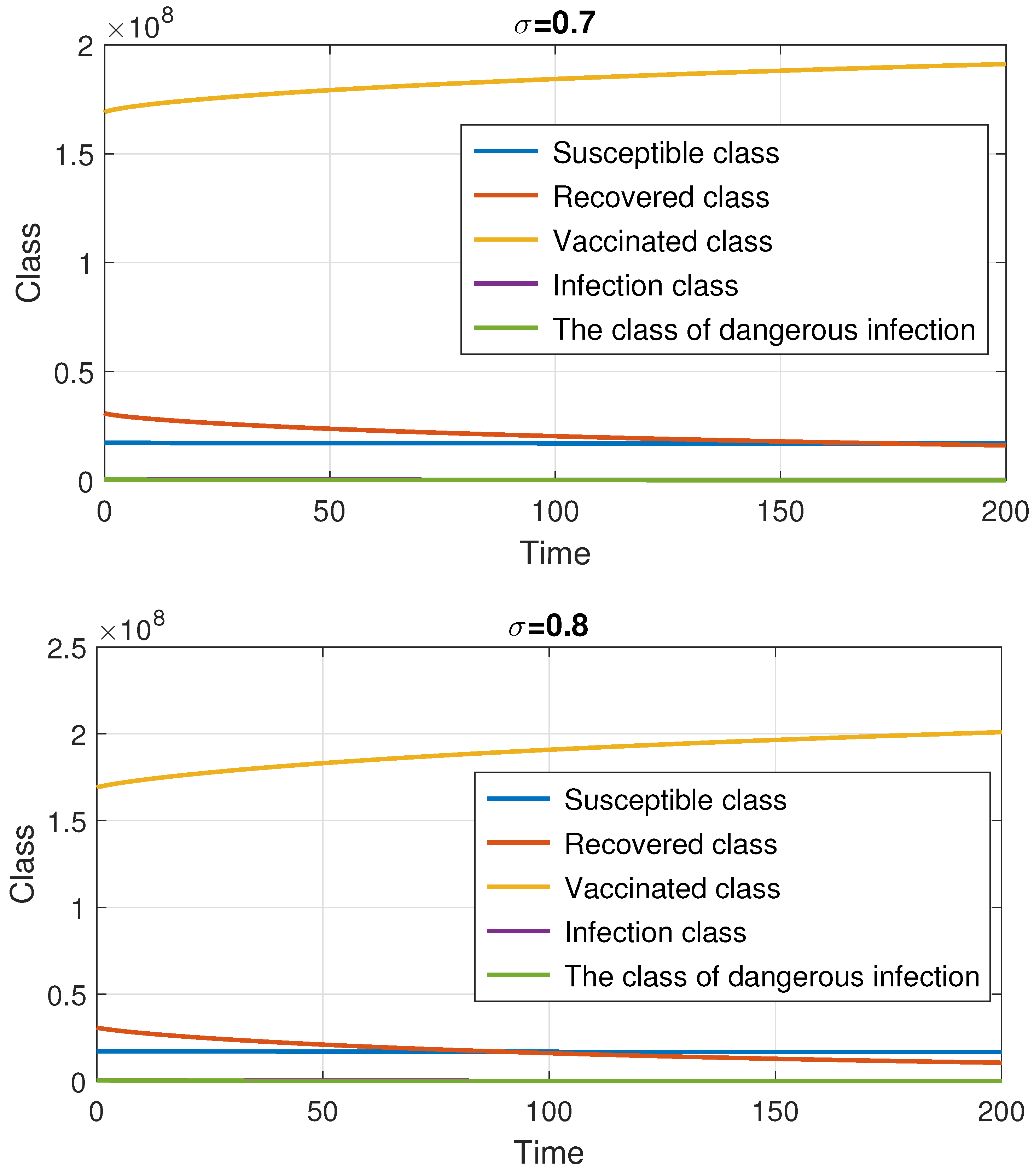
Figure 1. Time evolution of the COVID-19 model compartments for different values of the fractional order σ at ζ = 200 . Decreasing the fractional order σ (stronger memory) slows the transient response and spreads infections over a longer horizon, which lowers the peak in the severe class I d relative to σ = 1 while increasing the persistence of mild infections I . Vaccination shifts mass from S and R into V , reducing effective transmissions through the smaller breakthrough rate ρ 3 . Across all σ , the total population stays bounded by Θ / γ (invariant region), and trajectories remain in the nonnegative orthant, in agreement with the analytical results.
Mathematics 13 03619 g001aMathematics 13 03619 g001b
Table 1. Description of model variables and parameters.
SymbolMeaning
Θ Rate at which new individuals enter S
χ Proportion of infected individuals with mild symptoms
ρ 1 Infection rate from I and I d to S
ρ 2 Reinfection rate from I and I d to R
ρ 3 Infection rate for vaccinated individuals in V
β Vaccination rate for S and R
ε Rate at which individuals recover (from I and I d to R )
γ Natural mortality rate
δ Epidemic-related death rate (applies to I d )
μ Average number of contacts per individual per unit time
p i Probability of infection (subscript i indicates the class)
Disclaimer/Publisher’s Note: The statements, opinions and data contained in all publications are solely those of the individual author(s) and contributor(s) and not of MDPI and/or the editor(s). MDPI and/or the editor(s) disclaim responsibility for any injury to people or property resulting from any ideas, methods, instructions or products referred to in the content.