An IPNN-Based Parameter Identification Method for a Vibration Sensor Sensitivity Model

Abstract

Vibration sensors, as critical components in motion control and measurement systems, have dynamic characteristics that directly affect measurement accuracy. However, existing sensitivity models, due to structural simplifications and parameter uncertainties, hinder conventional vibration and shock calibration methods from fully characterizing their dynamic performance. In addition, traditional parameter identification approaches are often noise-sensitive and lack interpretability, making them inadequate for high-precision applications. To address these challenges, this study proposes an Algorithm-Unrolled Interpretable Physics-Informed Neural Network (IPNN) for parameter identification of a vibration sensor sensitivity model. By integrating the physical characteristics of the sensors with vibration calibration data, the method enables high-precision parameter identification and interpretable dynamic modeling. Comparative experimental results show that the proposed IPNN reduces the RMSE of sensor voltage predictions by over 60% compared with GRU and LSTM and decreases the average full-frequency relative deviation from laser interferometry calibration results by approximately 65% relative to LSM.

1. Introduction

Vibration sensors have been widely used to measure the displacement, velocity, and acceleration of structures, playing a critical role in applications such as machinery fault diagnosis, seismic monitoring, and structural health monitoring of large-scale buildings [1,2,3]. Their dynamic characteristics directly affect the reliability of these applications, making effective dynamic calibration essential prior to use. Currently, the calibration of vibration sensors is primarily performed using vibration and shock excitation methods [4,5,6,7,8]. Vibration calibration using sinusoidal excitation obtains sensitivity at a single frequency, which is difficult to directly apply to time-domain transient signal measurements. Calibration with shock excitation yields peak ratio results that are highly dependent on the excitation waveform, making it challenging to fully match actual measurements. Although current calibration methods can achieve reliable results under specific conditions, they are limited in comprehensively characterizing the dynamic behavior of sensors and cannot meet the requirements of high-precision dynamic measurements.

In recent years, calibration methods based on model parameter identification have become a research focus, treating vibration sensors as dynamic systems and identifying the sensitivity model parameters using vibration and shock calibration data. The modeling of sensitivity models mainly includes mechanistic modeling, data-driven modeling, and hybrid modeling, which respectively rely on physical mechanisms, calibration data fitting, or a combination of both to improve model accuracy [9,10,11,12,13,14,15]. However, due to differences in sensor structures and materials, these modeling approaches still involve structural simplifications and parameter uncertainties, resulting in relatively large model errors. In terms of parameter identification, methods can be mainly divided into time-domain and frequency-domain approaches. The former identifies model parameters using shock calibration data, which can handle complex dynamic signals effectively but requires high data quality and algorithmic convergence [16,17]. The latter relies on sinusoidal calibration data to identify model parameters using algorithms such as least squares, requiring less data but being susceptible to spectral leakage, noise, and nonlinearity, resulting in relatively large identification errors [18,19].

Deep learning, due to its powerful nonlinear fitting capability, automatic feature extraction, and end-to-end optimization characteristics, has been widely applied to system modeling and parameter identification [20,21,22,23,24]. Verhoek et al. [25] proposed a deep learning-based Linear Parameter-Varying (LPV) model identification method, which combines deep neural networks (DNNs) with a physical model to effectively identify the aerodynamic parameters of aircraft, demonstrating the potential of deep learning in the identification of time-varying linear systems. Caforio et al. [26] employed Physics-Informed Neural Networks (PINNs) to estimate the material parameters of a soft tissue biomechanical model, significantly improving model accuracy and physical consistency. Lin et al. [27] applied PINNs for the identification of aerodynamic parameters of aircraft, effectively enhancing the prediction accuracy of aerodynamic parameters. Zhao et al. [28] proposed a Deep Sparse Regression Network (DSRN)-based method for nonlinear dynamic system identification, enabling more precise capture of the system’s nonlinear characteristics. Additionally, Raissi et al. [29] introduced the foundational PINN framework for solving forward and inverse problems involving nonlinear partial differential equations, highlighting the ability of PINNs to incorporate physical laws into deep learning. Sorrentino et al. [30] combined PINNs with an Unscented Kalman Filter for sensorless joint torque estimation in humanoid robots, illustrating the integration of physics-informed networks with estimation techniques in complex dynamical systems. Although these deep learning methods have shown excellent performance in modeling and parameter identification, they generally suffer from a lack of interpretability, a strong dependence on large amounts of high-quality data, a tendency to overfit, and high computational complexity, which limit their feasibility in engineering applications [29,31,32].

To address the above issues, this study proposes a vibration sensor sensitivity model parameter identification method based on an Interpretable Physics-Informed Neural Network (IPNN), which effectively determines the sensitivity model parameters and achieves interpretable dynamic modeling, thereby ensuring the reliability of vibration sensor application systems. Furthermore, this framework also shows potential applicability to SHM-oriented studies using vibration sensors and hybrid optimization techniques, similar to applications reported in the recent literature [33,34,35].

The remainder of this paper is organized as follows. Section 2 introduces the discrete state-space model of vibration sensor sensitivity. Section 3 describes the principle of the IPNN based on algorithm unrolling. Section 4 presents simulation experiments to verify the high-accuracy performance of the proposed method in sensitivity model parameter identification. Section 5 provides a comparison with laser interferometric calibration experiments and discusses the results. Finally, Section 6 concludes the paper.

2. Discrete State-Space Model of Vibration Sensor Sensitivity

2.1. Sensitivity Model

Within the approximately linear range of sensitivity characteristics, the equivalent physical model of a vibration sensor can typically be represented as a single-degree-of-freedom mass–spring–damper system, as shown in Figure 1, although multi-degree-of-freedom or non-linear models may offer higher accuracy at the cost of increased complexity.

A mass block of mass m is housed within the vibration sensor casing and is supported by a spring with stiffness k and a damper with damping coefficient c. The vibration sensor is mounted on the measured structure, and when the sensor moves with the structure, the mass block undergoes displacement relative to the casing. Its motion can be described by the following equation:

$$c(\dot{S}(t)-\dot{R}(t))+k(S(t)-R(t))=m\ddot{R}(t)$$

(1)

In this equation, R(t) denotes the displacement of the mass block relative to the inertial reference frame, and S(t) denotes the displacement of the sensor base relative to the inertial reference frame.

The displacement of the mass block relative to the vibration sensor base is $x\left(t\right)=S\left(t\right)-R\left(t\right)$, and the sensor output signal is proportional to this displacement, i.e., $V\left(t\right)=Kx\left(t\right)$, where K is the conversion coefficient from displacement to output signal. If the sensor is subjected to an excitation acceleration $a\left(t\right)=\ddot{S}\left(t\right)$, the sensitivity model of the sensor can be expressed as:

$$\ddot{V}(t)+2\delta {\omega }_n\dot{V}(t)+{\omega }_n^{2}V(t)=Ka(t)$$

(2)

Here, $\delta =c/\left(2\sqrt{km}\right)$ is the equivalent damping ratio of the sensor, and ${\omega }_n=\sqrt{k/m}$ is the natural angular frequency of the sensor. K is the conversion coefficient, which can be expressed as $K=S_0{\omega }_n^2$, where $S_0$ is the sensitivity at the reference point. The relationship between the natural frequency and the resonant angular frequency is given by

$${\omega }_n={\displaystyle \frac{{\omega }_r}{\sqrt{1-2{\delta }^2}}}$$

(3)

In this equation, ${\omega }_r=2·\pi ·f_0$ denotes the resonant angular frequency, and $f_0$ denotes the resonant frequency.

2.2. Continuous-Time State-Space Model

A state-space model is a lumped-parameter model that simplifies the system based on the vibration sensor sensitivity model into state, input, and output variables. Combining Equations (1) and (2), the mass block’s relative displacement and velocity ${\left[x\left(t\right)\dot{x}\left(t\right)\right]}^T$ with respect to the sensor base are taken as state variables. Since the sensor output signal is proportional to this displacement, a new state variable ${\left[V\left(t\right)\dot{V}\left(t\right)\right]}^T$ is defined. Meanwhile, the acceleration excitation signal $a\left(t\right)$ of the sensor is defined as the input variable, and the sensor output signal $V\left(t\right)$ as the output variable. Accordingly, the state-space model of the sensor sensitivity can be expressed as:

$$\left\{\begin{array}{l}\left[\begin{array}{c}\dot{V}(t)\\ \ddot{V}(t)\end{array}\right]=\mathit{A}\left[\begin{array}{c}V(t)\\ \dot{V}(t)\end{array}\right]+\mathit{B}a(t)=\left[\begin{array}{cc}0& 1\\ {\omega }_n^2& -2\delta {\omega }_n\end{array}\right]\left[\begin{array}{c}V(t)\\ \dot{V}(t)\end{array}\right]+\left[\begin{array}{c}0\\ K\end{array}\right]a(t)\hfill \\ V(t)=\mathit{C}\left[\begin{array}{c}V(t)\\ \dot{V}(t)\end{array}\right]=\left[\begin{array}{cc}1& 0\end{array}\right]\left[\begin{array}{c}V(t)\\ \dot{V}(t)\end{array}\right]\hfill \end{array}\right.$$

(4)

According to state-space theory, the system matrix of the sensitivity state-space model is denoted as A, the input matrix as B, and the output matrix as C. Since both the controllability matrix ${\mathit{Q}}_{\mathit{c}}=\left[\mathit{B}\mathit{B}\mathit{A}\right]$ and the observability matrix ${\mathit{Q}}_{\mathit{o}}={\left[\mathit{C}\mathit{C}\mathit{A}\right]}^{\mathit{T}}$ are of full rank, the dynamic system of the vibration sensor is completely controllable and observable.

2.3. Discrete-Time State-Space Model

To reduce the errors caused by the structural simplification of the sensitivity model, the state-space model is discretized using the forward Euler method. Accordingly, the discrete-time state-space model can be expressed as:

$$\left\{\begin{array}{l}V(k+1)=(\mathit{I}+T_s\mathit{A})V(k)+T_s\mathit{B}a(k)\hfill \\ V(k)=\mathit{C}V(k)+\mathit{D}a(k)\hfill \end{array}\right.$$

(5)

In this equation, $T_s$ denotes the sampling period, and k denotes the k-th discrete time point.

By substituting $V(k+1)$ into the output equation of the discrete-time state-space model, we obtain:

$$\left\{\begin{array}{l}V(k+1)=(\mathit{I}+T_s\mathit{A})V(k)+T_s\mathit{B}a(k)\hfill \\ V(k)=\mathit{C}{(\mathit{I}+T_s\mathit{A})}^{-1}V(k+1)+(\mathit{D}-\mathit{C}{(\mathit{I}+T_s\mathit{A})}^{-1}{T}_s\mathit{B})a(k)\hfill \end{array}\right.$$

(6)

Based on Equations (4) and (6), the discrete-time state-space model of the sensor sensitivity can be established and expressed as:

$$\left\{\begin{array}{l}\left[\begin{array}{c}{V}^{(k+1)}\\ {\dot{V}}^{(k+1)}\end{array}\right]={\mathit{A}}_{\mathit{d}}\left[\begin{array}{c}{V}^{(k)}\\ {\dot{V}}^{(k)}\end{array}\right]+{\mathit{B}}_{\mathit{d}}a(k)=\left[\begin{array}{cc}1& T_s\\ {\omega }_n^2{T}_s& 1-2\delta {\omega }_n{T}_s\end{array}\right]\left[\begin{array}{c}{V}^{(k)}\\ {\dot{V}}^{(k)}\end{array}\right]+\left[\begin{array}{c}0\\ K{T}_s\end{array}\right]a(k)\hfill \\ V(k)={\mathit{C}}_{\mathit{d}}\left[\begin{array}{c}{V}^{(k+1)}\\ {\dot{V}}^{(k+1)}\end{array}\right]+{\mathit{D}}_{\mathit{d}}a(k)=\gamma \left[\begin{array}{cc}1-2\delta {\omega }_n{T}_s& -T_s\end{array}\right]\left[\begin{array}{c}{V}^{(k+1)}\\ {\dot{V}}^{(k+1)}\end{array}\right]+\gamma \lambda T_s^{2}a(k)\hfill \end{array}\right.$$

(7)

In this equation, $\gamma =1/(1-2\delta {\omega }_n-{\omega }_n^2{T}_s^2)$ ${\mathit{A}}_{\mathit{d}}$, ${\mathit{B}}_{\mathit{d}}$, ${\mathit{C}}_{\mathit{d}}$, ${\mathit{D}}_{\mathit{d}}$ denote the state transition matrix, control input matrix, output matrix, and direct transmission matrix of the discrete-time state-space model, respectively.

Based on the above analysis, discretizing the sensitivity model into state-space form not only reduces the errors caused by structural simplification but also provides physical constraints and a structural basis for the construction of an interpretable physics-informed neural network.

3. Principle of the Interpretable Physics-Informed Neural Network Based on Algorithm Unrolling

3.1. Algorithm-Unrolled Interpretable Deep Learning Network

Gregor and LeCun proposed the algorithm unrolling technique [36], which achieves the interpretability of deep learning networks by mapping iterative optimization algorithms into neural network architectures. The structural framework is displayed in Figure 2. Specifically, Figure 2a illustrates an iterative optimization process. By cascading the iterative steps, a corresponding deep network can be constructed, as displayed in Figure 2b. The algorithm parameters involved in each iteration are directly mapped to the weight parameters in the network layers. Unlike traditional methods that determine parameters through analytical derivation or cross-validation, algorithm unrolling learns the optimal parameter configuration directly from data via end-to-end training, enabling the network to outperform the original iterative algorithm. Meanwhile, since each network layer corresponds to a specific iteration step, this method naturally inherits the interpretability of the iterative process.

Compared with traditional neural networks, algorithm-unrolled networks contain fewer parameters, require less training data, and can directly incorporate physical priors and domain knowledge without relying on large-scale data-driven learning, thereby exhibiting superior generalization capability.

3.2. IPNN Based on the Discrete State-Space Model

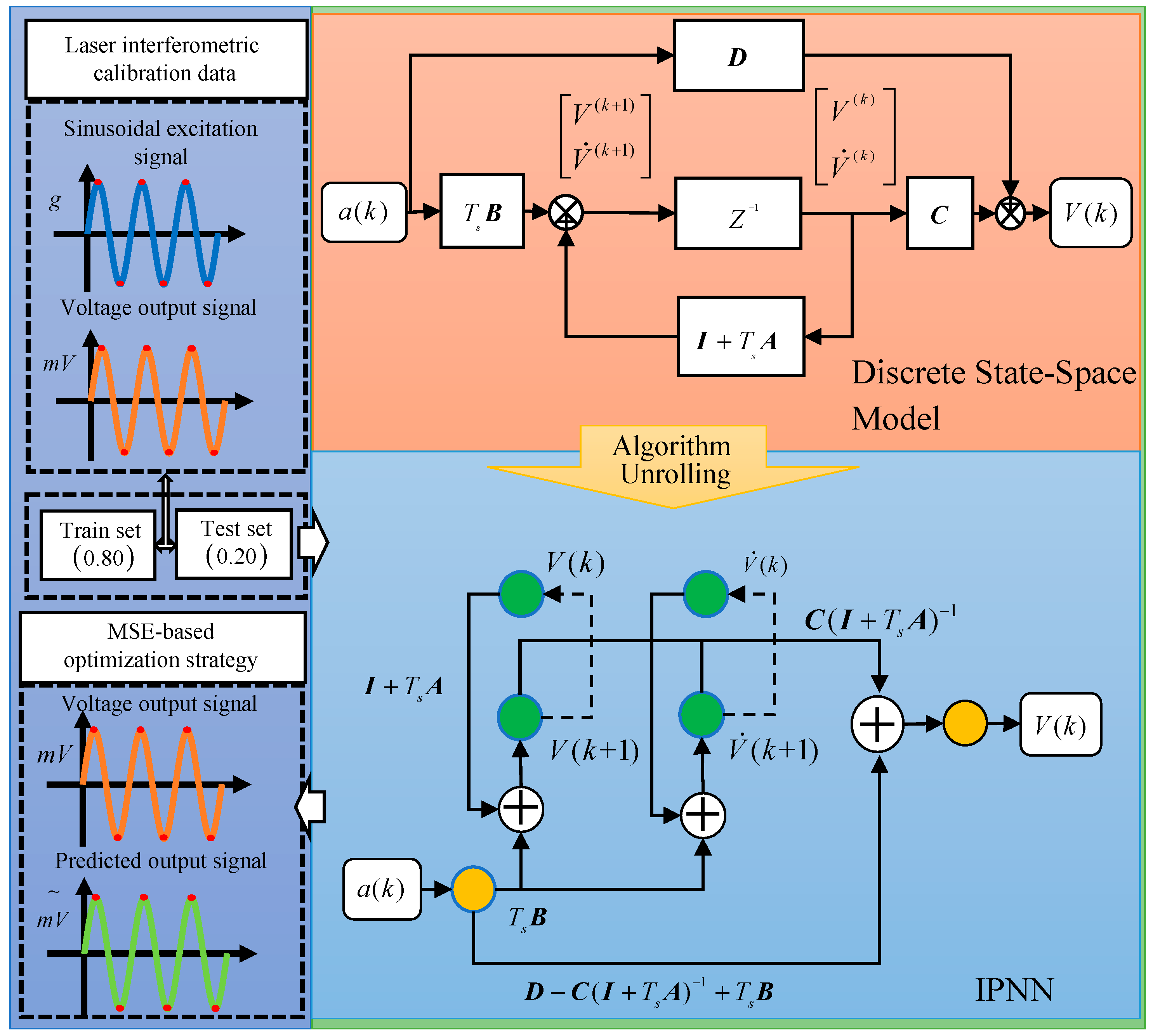
In this study, the concept of algorithm unrolling is combined with the discrete state-space model of the vibration sensor to construct a fully interpretable physics-informed neural network, as shown in Figure 3. The network offers clear advantages in physical consistency, parameter interpretability, and model stability. It preserves the benefits of deep learning for dynamic modeling while incorporating the sensor’s physical characteristics, achieving full interpretability.

The IPNN comprises an input layer, a feedback layer, a hidden layer, a feedforward layer, and an output layer, with 1, 2, 2, 1, and 1 neurons, respectively. The layer weights directly correspond to the physical parameters in the discrete state-space model, as listed in

Table 1. Equivalence between the IPNN and the Discrete State-Space Model.

IPNN	Weight Parameters	Discrete State-Space Model
Input layer	W1	${\mathit{B}}_{\mathit{d}}=T_s\mathit{B}$
Hidden layer	W2	${\mathit{A}}_{\mathit{d}}=\mathit{C}{(\mathit{I}+T_s\mathit{A})}^{-1}$
Feedback layer	W3	${\mathit{C}}_{\mathit{d}}=(\mathit{I}+T_s\mathit{A})$
Feedforward layer	W4	${\mathit{D}}_{\mathit{d}}=(\mathit{D}-\mathit{C}{(\mathit{I}+T_s\mathit{A})}^{-1}{T}_s\mathit{B})$

.

Based on the equivalence between the IPNN and the discrete state-space model provided in Table 1, the following equations can be derived:

$$\left\{\begin{array}{l}{\mathit{W}}_1={\mathit{B}}_{\mathit{d}}=T_s\mathit{B}\hfill \\ {\mathit{W}}_2={\mathit{A}}_{\mathit{d}}=\mathit{C}{(\mathit{I}+T_s\mathit{A})}^{-1}\hfill \\ {\mathit{W}}_3={\mathit{C}}_{\mathit{d}}=(\mathit{I}+T_s\mathit{A})\hfill \\ {\mathit{W}}_4={\mathit{D}}_{\mathit{d}}=(\mathit{D}-\mathit{C}{(\mathit{I}+T_s\mathit{A})}^{-1}{T}_s\mathit{B})\hfill \end{array}\right.$$

(8)

where A_d, B_d, C_d, and D_d represent the state transition matrix, control input matrix, output matrix, and direct transmission matrix of the discrete state-space model, respectively.

In practical implementation, the proposed IPNN is trained end-to-end using a dataset containing vibration calibration data. The network weights quickly converge, achieving optimal prediction performance. By combining Equations (7) and (8), the unknown parameters of the sensitivity model can be accurately identified.

Thus, the vibration sensor sensitivity model parameter identification method based on the IPNN is fully established. This method takes the discrete state-space equations as its core and integrates the concept of algorithm unrolling to construct a fully interpretable physics-informed neural network, achieving a unified framework of physical consistency, parameter interpretability, and model stability.

4. Simulation Validation

4.1. Dataset Description and Parameter Settings

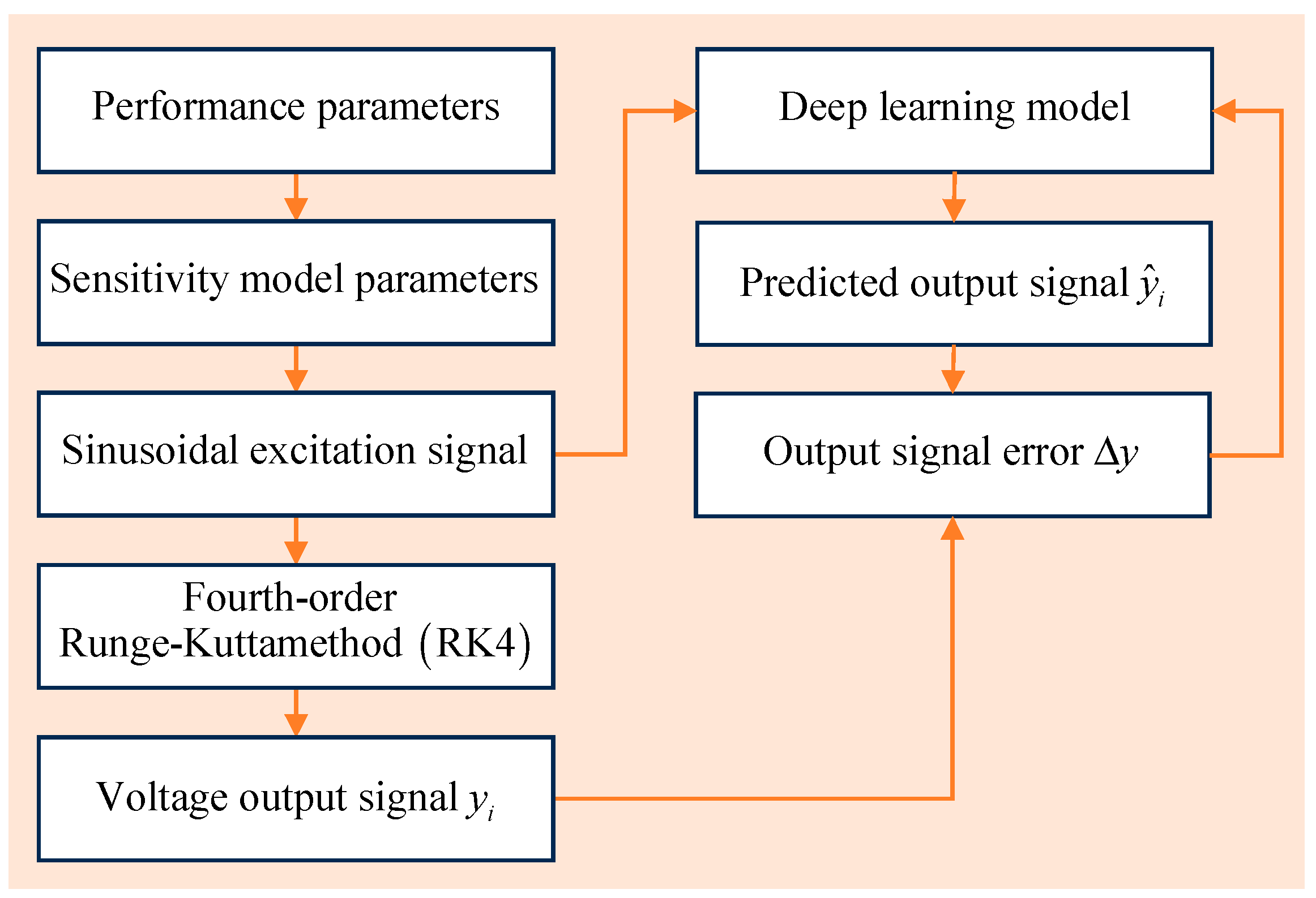
The process for generating vibration calibration simulation data was illustrated in Figure 4. The dataset contained sinusoidal excitation signals and voltage output signals of the vibration sensor, with the former serving as the network input and the latter as the target output. This process was described as follows. First, the sensitivity model parameters were set based on the performance specifications of the vibration sensor. Second, sinusoidal waves were applied within the frequency range of 0.1–1000 Hz to simulate real environmental vibrations, with Gaussian white noise added to enhance the network’s robustness. Third, the vibration sensor sensitivity model was solved using the fourth-order Runge–Kutta (RK4) method to obtain the corresponding voltage output signals under the applied excitation. The sinusoidal excitation and voltage output signals were then normalized, and outliers were removed to construct the dataset, which was split into training and testing sets in an 8:2 ratio. The training set was used for model training, while the testing set was used for performance evaluation. The resulting dataset contained 21 samples, covering the low-frequency range, resonance region, and high-frequency range, thus comprehensively reflecting the dynamic response characteristics of the sensor.

According to the vibration sensor’s technical manual, performance parameters, including the resonance frequency and low-frequency reference sensitivity, were obtained. Using Equation (3), the natural angular frequency and the conversion coefficient of the sensitivity model were calculated, while the damping ratio was set based on empirical values. The complete set of sensitivity model parameters was provided in

Table 2. Vibration Sensor Performance Parameters and Sensitivity Model Parameters.

Resonance Frequency (Hz)	Reference Sensitivity (mV/g)	Damping Ratio	Natural Angular Frequency (rad/s)	Conversion Coefficient (mV/mm)
630	1020	0.182	4.10 × 103	1.63 × 106

.

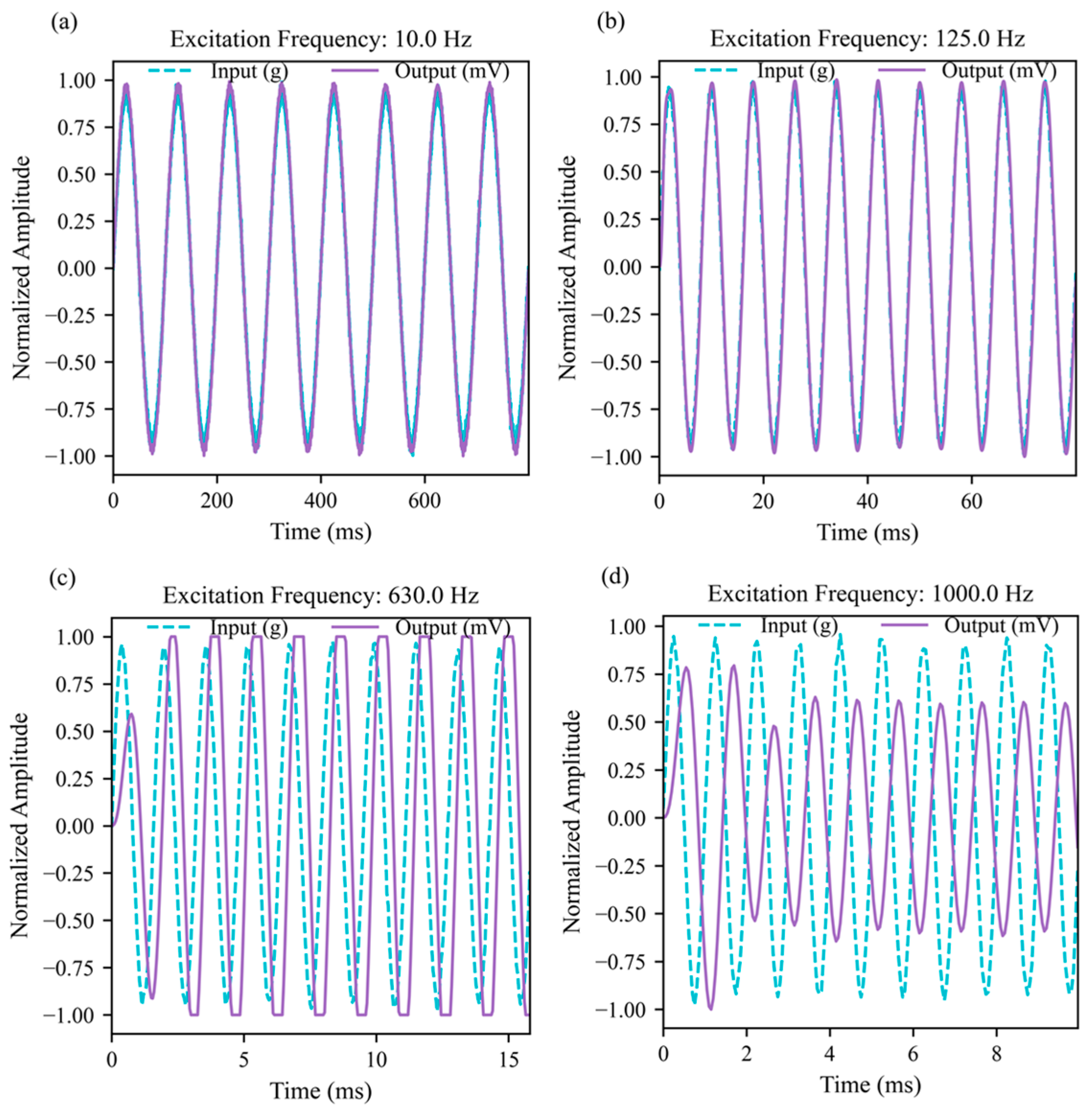
According to the center frequency divisions specified in the ISO standard [37], a frequency sequence was generated in the range of 0.1–1000 Hz using one-third octave spacing. A sinusoidal signal with an amplitude of 1 g was applied as the excitation, with 20 dB Gaussian white noise superimposed to simulate real environmental vibration conditions. Both the excitation and voltage output signals were normalized to the range of [–1, 1] using the min–max normalization method, expressed as $x_{norm}=2\ast {\displaystyle \frac{{x-x}_{min}}{x_{max}-x_{min}}}-1$, which can eliminate the amplitude scaling influence. Each input sample contained 16,000 time-domain data points for the excitation and output signals used for the model training. Figure 5 shown the sinusoidal excitation signal and its corresponding voltage output at typical frequencies.

To verify whether the proposed discrete state-space sensitivity model could fully capture the dynamic characteristics of the vibration sensor, the sensitivity was calculated based on the sinusoidal excitation and voltage output signals, and the sensitivity curves were plotted, as displayed in Figure 6. Comparison with the reference sensitivity indicated that the proposed model accurately reflected the sensor’s dynamic response and effectively reduced the modeling errors introduced by structural simplifications in conventional models.

4.2. Validation Results

To evaluate the performance of the IPNN, numerical comparison experiments were conducted with commonly used time-series prediction models, namely the Long Short-Term Memory (LSTM) network and the Gated Recurrent Unit (GRU) network. The models’ performance in predicting voltage output signals was quantitatively evaluated using Root Mean Square Error (RMSE), Mean Absolute Error (MAE), Mean Squared Error (MSE), Coefficient of Determination (R²), and the Ratio of Performance to Deviation (RPD). RMSE and MSE reflect the overall deviation between predicted and true values, with smaller values indicating higher accuracy. MAE represents the mean absolute error, measuring the average deviation of the predictions. R² indicates the goodness of fit of the model, with values closer to 1 representing a better fit. RPD assesses the model’s generalization capability, with RPD > 3 generally considered to indicate highly reliable predictions. The formulas for these metrics are as follows:

$$RMSE=\sqrt{{\displaystyle \frac{1}{N}}{\displaystyle \sum _{i=1}^N{(y_i-{\widehat{y}}_i)}^2}}$$

(9)

$$MAE={\displaystyle \frac{1}{N}}{\displaystyle \sum _{i=1}^N\left|y_i-{\widehat{y}}_i\right|}$$

(10)

$$MSE={\displaystyle \frac{1}{N}}{\displaystyle \sum _{i=1}^N{(y_i-{\widehat{y}}_i)}^2}$$

(11)

$$R^2=1-{\displaystyle \frac{{\displaystyle {\sum }_{i=1}^N{\left(y_i-{\widehat{y}}_i\right)}^2}}{{\displaystyle {\sum }_{i=1}^N{\left(y_i-\overline{y_i}\right)}^2}}}$$

(12)

$$RPD={\displaystyle \frac{SD(y)}{RMSE}}$$

(13)

where $y_i$ is the actual voltage output of the vibration sensor, $\widehat{y_i}$ is the voltage output predicted by the deep learning network, $\overline{y}$ is the mean of the actual voltage outputs, and N is the total number of data points in the dataset.

The model was trained using the Adam optimizer with the MSE loss function on an Intel Core i7-13700KF CPU. The optimal hyperparameters were listed in

Table 3. The optimal hyperparameters of the three models are summarized.

Hyperparameter	IPNN	LSTM	GRU
Learning Rate	0.001	0.001	0.001
Batch Size	36	36	36
Activation Function	Tanh	Tanh	Tanh
Bias	None	None	None
Hidden Layers	1	16	16

.

The prediction performance on the test set is provided in

Table 4. Prediction Performance of Voltage Output Signals for the Three Models.

Comparison Methods	RMSE	MAE	MSE	R2	RPD
GRU	0.0136	0.0111	0.0035	0.9900	10.4982
LSTM	0.0244	0.0235	0.0101	0.9115	5.8490
IPNN	0.0061	0.0069	0.0035	0.9919	23.1757

. The results showed that all three models had RPD values greater than 3, indicating reliable predictions. Among them, the IPNN outperformed the LSTM and GRU models in terms of RMSE, MAE, and R², demonstrating higher accuracy in voltage signal prediction and providing a solid foundation for the high-precision identification of sensitivity model parameters.

To further validate the effectiveness of the IPNN in sensitivity model parameter identification, a comparative analysis was conducted using the Least Squares Method (LSM). Figure 7 shows the theoretical sensitivity curve along with the sensitivity results calculated using parameters identified by the IPNN and LSM. The results indicated that the IPNN closely matches the theoretical sensitivity across the entire frequency range, accurately capturing the resonance peak, whereas the LSM exhibits deviations in the high-frequency range, underestimating the peak. Quantitatively, the average relative deviation of the IPNN from the theoretical sensitivity over the full frequency range was only 0.55%, approximately 75% lower than that of the LSM, and the maximum deviation at the resonance peak was merely 1.25%, significantly better than the 3.5% that was observed with the Least Squares Method. The analysis indicated that the IPNN achieved higher accuracy and reliability in sensitivity calibration.

5. Experimental Validation and Results Analysis

5.1. Experimental Setup and Dataset Description

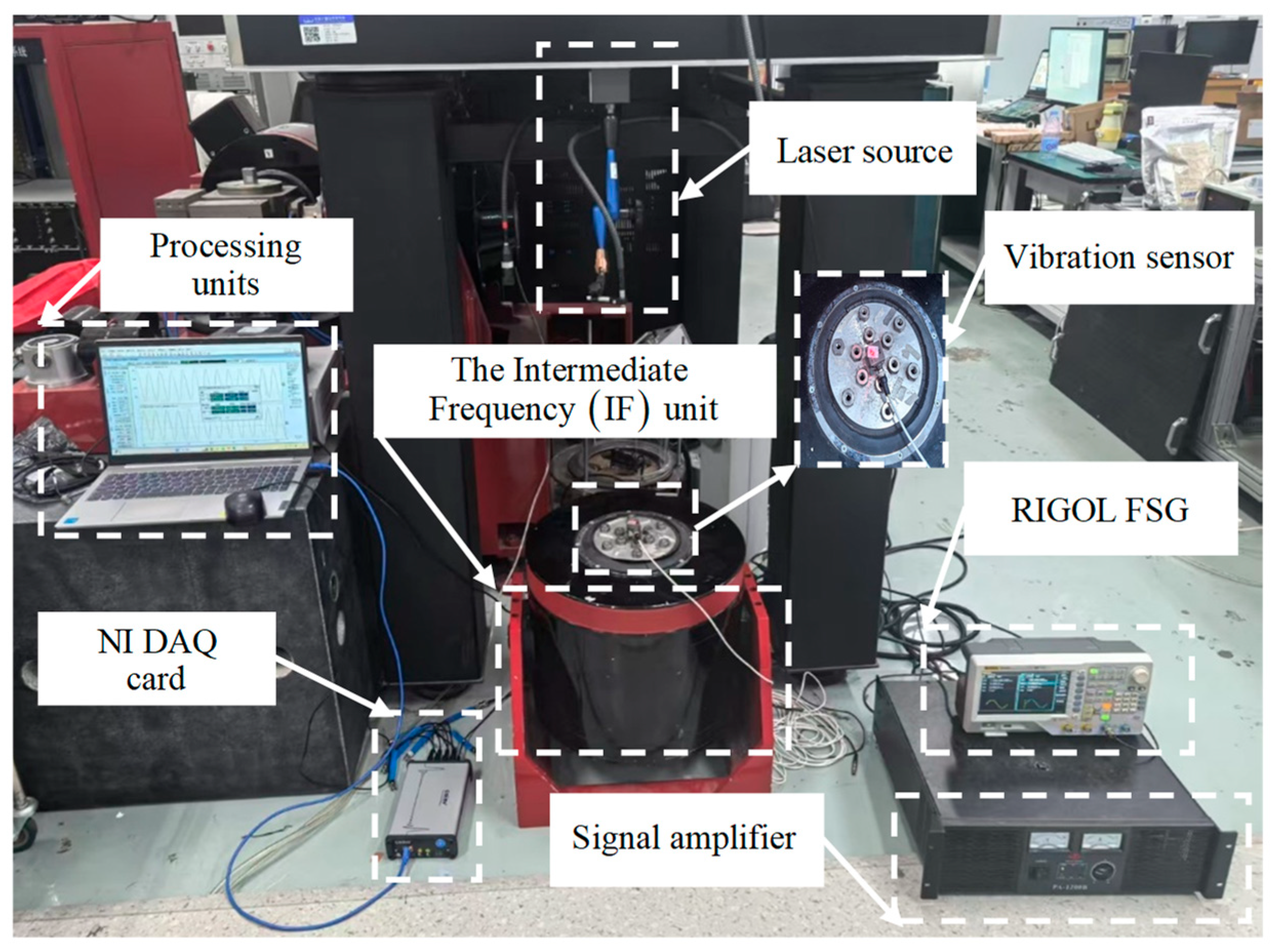
In this study, a Laser Interferometry (LI) calibration system was used to measure the sinusoidal excitation and voltage output signals of the vibration sensor. The experimental setup was shown in Figure 8. A signal generator (RIGOL DG 4202) was used to produce the sinusoidal excitation signal, which was amplified by a power amplifier (PA-1200B). A mid-frequency shaker (FS-050-150) provided the vibration sensor under test (MSV 3000) with sinusoidal excitation in the frequency range of 0.1–1000 Hz. A laser interferometer (OFV-552, sensitivity 50 (mm/s)/V) and a DAQ card (INV-3608P) were employed to simultaneously measure the excitation and output signals of the vibration sensor.

Subsequently, following the same dataset construction method used in the simulation experiments, the acquired voltage excitation and output signals were preprocessed to create a dataset for vibration sensor sensitivity model parameter identification. The dataset was then split into training and testing sets in an 8:2 ratio. The final dataset contained 21 samples, covering the low-frequency range, resonance region, and high-frequency range, thus comprehensively reflecting the dynamic response characteristics of the sensor.

5.2. Experimental Validation Results

Table 5. Prediction Performance of Voltage Output Signals for the Three Models.

Comparison Methods	RMSE	MAE	MSE	R2	RPD
GRU	0.0252	0.0859	0.0135	0.9608	8.4325
LSTM	0.0468	0.0753	0.0101	0.9115	4.4277
IPNN	0.0099	0.0069	0.0035	0.9919	12.3441

provides a performance comparison of the predicted voltage output signals of the vibration sensor. The results indicated that the IPNN outperformed the GRU and LSTM across all five evaluation metrics, demonstrating lower prediction errors, higher fitting accuracy, and stronger generalization and stability. This provided a reliable basis for the subsequent high-precision identification of sensitivity model parameters using the IPNN.

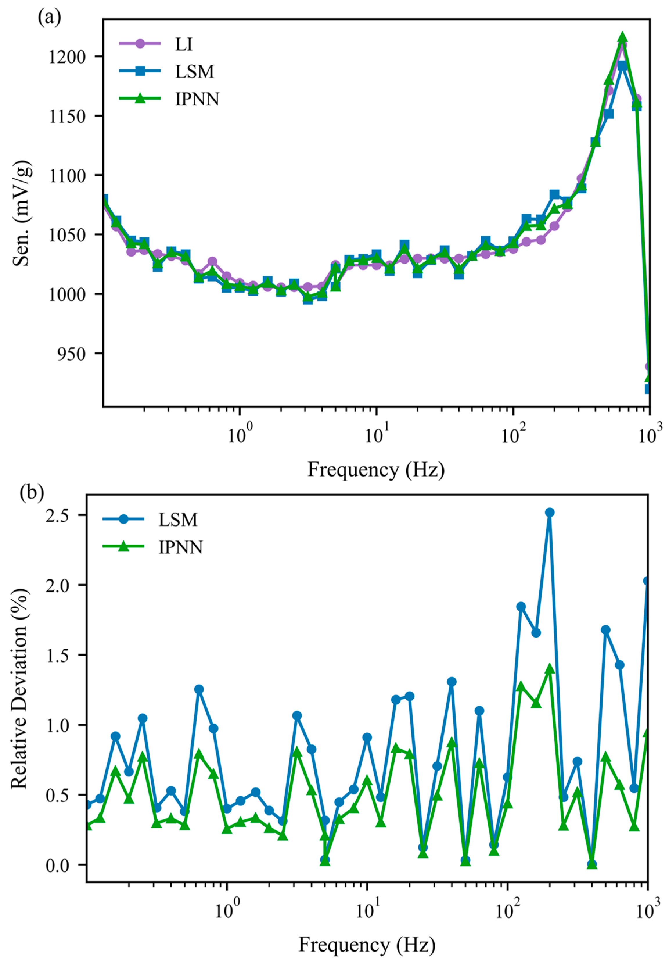
Figure 9 displayed the sensitivity curves obtained from laser interferometry calibration and the sensitivity calculated using parameters identified by the IPNN and LSM. The results indicated that the IPNN aligned closely with the LI calibration results across the entire frequency range, particularly capturing the resonance peak accurately, whereas the LSM showed deviations in the high-frequency range, underestimating the peak. Quantitative analysis revealed that the IPNN’s average relative deviation from the LI calibration results over the full frequency range was only 0.88%, approximately 65% lower than that of the Least Squares Method, with a maximum deviation of just 1.4%, significantly better than LSM’s 2.51%. These findings demonstrated that the IPNN achieved higher accuracy and reliability in sensitivity calibration.

5.3. Discussion

The experimental results in Figure 9 indicated that the IPNN exhibited lower prediction errors and higher fitting accuracy across the low-frequency range, resonance region, and high-frequency range. This performance can be mainly attributed to the following factors: (I) The embedding of physical priors discretized the sensor’s dynamic equations into state-space form and integrated them into the network structure, ensuring that the model maintained adhered to physical constraints across the entire frequency range, thereby reducing degrees of freedom and suppressing deviations caused by noise; (II) The deep learning component specifically captured the residual dynamics not captured by the physical model, effectively compensating for amplitude underestimation in the resonance region and prediction errors at high frequencies. Ultimately, the synergy of both components enabled the IPNN to maintain low RMSE and average relative deviation across the entire frequency range, significantly outperforming the LSM, GRU, and LSTM, demonstrating its high accuracy and stability in vibration sensor sensitivity identification and voltage signal prediction.

6. Conclusions

This study proposed a vibration sensor sensitivity model parameter identification method based on an Interpretable Physics-Informed Neural Network (IPNN) to enhance parameter identification and interpretable dynamic modeling of the sensitivity model. Both numerical validation and comparison experiments with LI indicated that the IPNN outperformed the GRU and LSTM in terms of accuracy and stability for voltage output signal prediction, with the LSTM exhibiting the poorest performance. The sensitivity curve calculated using parameters identified by the IPNN closely aligned with the LI results, with an average relative deviation of only 0.88% across the full frequency range—approximately 65% lower than that of the LSM—and a maximum deviation of just 1.4%, significantly better than LSM’s 2.51%. These findings validated the advantages and reliability of the IPNN in sensitivity model parameter identification and interpretable dynamic modeling. In the future, this method can be integrated with various control systems to design more accurate control algorithms using the identified sensitivity model, thereby enhancing the dynamic performance of vibration sensors. Additionally, the interpretable structure and simple network architecture of the IPNN make it suitable for online learning and deployment in resource-constrained environments, such as embedded systems, and provide a promising direction for adaptive calibration and practical applications.

References

1. Guo, J.; He, Q.; Zhen, D.; Gu, F.; Ball, A.D. Multi-sensor data fusion for rotating machinery fault detection using improved cyclic spectral covariance matrix and motor current signal analysis. Reliab. Eng. Syst. Saf. 2023, 230, 108969. [Google Scholar] [CrossRef]
2. Qiu, Z.; Zhang, Y. Three-dimensional low-frequency earthquake monitoring vibration sensor based on FBG. IEEE Trans. Instrum. Meas. 2024, 73, 9510709. [Google Scholar] [CrossRef]
3. Parisi, E.; Moallemi, A.; Barchi, F.; Bartolini, A.; Brunelli, D.; Buratti, N.; Acquaviva, A. Time and frequency domain assessment of low-power MEMS accelerometers for structural health monitoring. In Proceedings of the 2022 IEEE International Workshop on Metrology for Industry 4.0 & IoT (MetroInd4.0 & IoT), Trento, Italy, 7–9 June 2022; IEEE: Piscataway, NJ, USA, 2022; pp. 1–6. [Google Scholar] [CrossRef]
4. ISO 16063-11; Methods for the Calibration of Vibration and Shock Transducers—Part 11: Primary Vibration Calibration by Laser Interferometry. International Organization for Standardization: Geneva, Switzerland, 1999.
5. Yang, M.; Cai, C.; Liu, Z.; Wang, Y. Monocular vision-based calibration method for determining frequency characteristics of low-frequency vibration sensors. IEEE Sens. J. 2021, 21, 4377–4384. [Google Scholar] [CrossRef]
6. Garg, N.; Sharma, O.; Kumar, A.; Schiefer, M.I. A novel approach for realization of primary vibration calibration standard by homodyne laser interferometer in frequency range of 0.1 Hz to 20 kHz. Measurement 2012, 45, 1941–1950. [Google Scholar] [CrossRef]
7. ISO 16063-41; Methods for the Calibration of Vibration and Shock Transducers—Part 41: Calibration of Laser Vibrometers. International Organization for Standardization: Geneva, Switzerland, 2001.
8. Wang, Q.; Xu, F.; Guo, W. Generation of wide-pulsewidth synchronous shocks and calibration for triaxial accelerometers. IEEE Trans. Instrum. Meas. 2024, 73, 1003116. [Google Scholar] [CrossRef]
9. Yang, Y.; Jiang, W.; Zhang, K.; Liu, M.; Li, X. A dynamic collision model for improved over-range protection of cantilever-mass micromechanical accelerometers. Microelectron. J. 2010, 41, 331–337. [Google Scholar] [CrossRef]
10. Hong, L.; Sun, R.; Qiu, Z.; Han, Z.; Li, Y. A multi-cantilever beam low-frequency FBG acceleration sensor. Sci. Rep. 2021, 11, 18502. [Google Scholar] [CrossRef]
11. Qiu, Z.; Su, K.; Zhang, J.; Sun, R.; Teng, Y. A miniaturized low-frequency FBG accelerometer based on symmetrical cantilever beam. IEEE Sens. J. 2023, 23, 5831–5840. [Google Scholar] [CrossRef]
12. Omran, A.; Newman, B. Generalized cause-and-effect analyses for the prototypic nonlinear mass–spring–damper system using Volterra kernels. J. Dyn. Syst. Meas. Control 2013, 135, 011008. [Google Scholar] [CrossRef]
13. Yu, T.; Hao, B.; Wang, J.; Zhao, L.; Wei, Q. An accelerometer modeling approach based on mixed-kernel support vector machine. In Proceedings of the 2016 12th World Congress on Intelligent Control and Automation (WCICA), Guilin, China, 12–15 June 2016; IEEE: Piscataway, NJ, USA, 2016; pp. 2760–2764. [Google Scholar] [CrossRef]
14. Wei, Q.; Wang, J.; Han, R.; Yu, T.; Zhao, L. Dynamic model parameter identification of accelerometer using discrete spectrum correction and least square. Trans. Beijing Inst. Technol. 2018, 38, 1282–1288. [Google Scholar] [CrossRef]
15. Chang, L.; Qin, F.; Jiang, S. Strapdown inertial navigation system initial alignment based on modified process model. IEEE Sens. J. 2019, 19, 6381–6391. [Google Scholar] [CrossRef]
16. Guo, C.; Shi, Y.; Cao, H.; Wen, X.; Zhao, R. Dynamic parameter identification of a high g accelerometer based on BP-PSO algorithm. Sens. Actuators A Phys. 2023, 349, 114024. [Google Scholar] [CrossRef]
17. Wang, Y.; Zhu, Z.; Huang, T.; Wu, B.; Song, K. High precision identification of dynamic model for accelerometer based on VMD. Measurement 2024, 237, 115226. [Google Scholar] [CrossRef]
18. Link, A.; Täubner, A.; Wabinski, W.; Bruns, T.; Elster, C. Modelling accelerometers for transient signals using calibration measurements upon sinusoidal excitation. Measurement 2007, 40, 928–935. [Google Scholar] [CrossRef]
19. Wu, B.; Huang, T.; Zhu, H.; Ye, L. Study of dynamic modeling method for quartz flexible accelerometer. In Proceedings of the 2015 12th IEEE International Conference on Electronic Measurement & Instruments (ICEMI), Qingdao, China, 16–18 July 2015; IEEE: Piscataway, NJ, USA, 2015; Volume 3, pp. 1477–1480. [Google Scholar] [CrossRef]
20. Song, B.-G.; Kang, N. Application of deep neural networks for the parameter identifications of lumped and distributed parameter models under severe noises and various initial values. J. Vib. Eng. Technol. 2024, 12, 3641–3652. [Google Scholar] [CrossRef]
21. Zhou, H.; Ibrahim, C.; Zheng, W.X.; Pan, W. Sparse Bayesian Deep Learning for Dynamic System Identification. Automatica 2022, 144, 110489. [Google Scholar] [CrossRef]
22. Dong, A.; Wang, P.; Liu, M. Neural Network-Based Parametric System Identification: A Review. Int. J. Syst. Sci. 2023, 54, 2345–2363. [Google Scholar] [CrossRef]
23. Niu, K.; Zhou, M.; Abdallah, C.T.; Hayajneh, M. Deep Transfer Learning for System Identification Using Long Short-Term Memory Neural Networks. arXiv 2022, arXiv:2204.03125. [Google Scholar] [CrossRef]
24. Kong, S.; Xu, L. A residual physics-informed neural network approach for identifying dynamic parameters in swing equation-based power systems. Energies 2025, 18, 2888. [Google Scholar] [CrossRef]
25. Verhoek, C.; Beintema, G.I.; Haesaert, S.; Schoukens, M.; Toth, R. Deep-learning-based identification of LPV models for nonlinear systems. In Proceedings of the 2022 IEEE 61st Conference on Decision and Control (CDC), Cancún, Mexico, 6–9 December 2022; IEEE: Piscataway, NJ, USA, 2022; pp. 3274–3280. [Google Scholar] [CrossRef]
26. Caforio, F.; Regazzoni, F.; Pagani, S.; Karabelas, E.; Augustin, C.; Haase, G.; Plank, G.; Quarteroni, A. Physics-informed neural network estimation of material properties in soft tissue nonlinear biomechanical models. Comput. Mech. 2025, 75, 487–513. [Google Scholar] [CrossRef]
27. Lin, J.; Chen, S.; Yang, H.; Jiang, Q.F.; Liu, J. A physics-informed neural network-based aerodynamic parameter identification method for aircraft. Phys. Fluids 2025, 37, 025109. [Google Scholar] [CrossRef]
28. Zhao, S.; Cheng, C.; Lin, M.; Peng, Z. Physics-informed deep sparse regression network for nonlinear dynamical system identification. J. Sound Vib. 2025, 595, 118796. [Google Scholar] [CrossRef]
29. Raissi, M.; Perdikaris, P.; Karniadakis, G.E. Physics-informed neural networks: A deep learning framework for solving forward and inverse problems involving nonlinear partial differential equations. J. Comput. Phys. 2019, 378, 686–707. [Google Scholar] [CrossRef]
30. Sorrentino, I.; Romualdi, G.; Moretti, L.; Traversaro, S.; Pucci, D. Physics-informed neural networks with Unscented Kalman Filter for sensorless joint torque estimation in humanoid robots. IEEE Robot. Autom. Lett. 2025, 10, 728–735. [Google Scholar] [CrossRef]
31. Samek, W.; Montavon, G.; Lapuschkin, S.; Anders, C.J.; Muller, K.-R. Explaining deep neural networks and beyond: A review of methods and applications. Proc. IEEE 2021, 109, 247–278. [Google Scholar] [CrossRef]
32. Montavon, G.; Samek, W.; Müller, K.R. Methods for interpreting and understanding deep neural networks. Digit. Signal Process. 2018, 73, 1–15. [Google Scholar] [CrossRef]
33. Mansouri, A.; Tiachacht, S.; Ait-Aider, H.; Khatir, S.; Khatir, A.; Cuong-Le, T. A novel Optimization-Based Damage Detection in Beam Systems Using Ad-vanced Algorithms for Joint-Induced Structural Vibrations. J. Vib. Eng. Technol. 2025, 13, 486. [Google Scholar] [CrossRef]
34. Jafari-Talookolaei, R.A.; Ghandvar, H.; Jumaev, E.; Mikhliev, O.; Khatir, S.; Cuong-Le, T. Dynamic Analysis of Two Straight and Curved Beams Connected with Intermediate Vertical Beams Made of Functionally Graded Porous Materials. Int. J. Struct. Stab. Dyn. 2025, 46, 37–62. [Google Scholar] [CrossRef]
35. Khatir, B.; Filali, S.; Belabdeli, S.; Daikh, A.A.; Khatir, S.; Capozucca, R.; Cuong-Le, T. Vibration analysis of new cosine functionally graded microplates using isogeometric analysis. Structures 2024, 69, 107467. [Google Scholar] [CrossRef]
36. Gregor, K.; LeCun, Y. Learning fast approximations of sparse coding. In Proceedings of the 27th International Conference on Machine Learning (ICML), Haifa, Israel, 21–24 June 2010; Omnipress: Madison, WI, USA, 2010; pp. 399–406. [Google Scholar] [CrossRef]
37. ISO 266:1997; Acoustics—Preferred Frequencies. International Organization for Standardization: Geneva, Switzerland, 1997.
Figure 1. Single-degree-of-freedom mass–spring–damper system.
Mathematics 13 03609 g001
Figure 2. Structure of the Algorithm-Unrolled Interpretable Deep Learning Network. (a) Illustration of the iterative optimization process. (b) Construction of a corresponding deep network by cascading the iterative steps. The algorithm parameters in each iteration are directly mapped to the network layer weights, enabling the network to learn the optimal configuration via end-to-end training.
Mathematics 13 03609 g002
Figure 3. Principle of the vibration sensor sensitivity model parameter identification network.
Mathematics 13 03609 g003
Figure 4. Dataset Preparation and Model Evaluation.
Mathematics 13 03609 g004
Figure 5. Sinusoidal Excitation and Voltage Output Signals at Typical Frequencies. (a) 10.0 Hz; (b) 125.0 Hz; (c) 630.0 Hz; (d) 1000.0 Hz.
Mathematics 13 03609 g005
Figure 6. Sensitivity Characteristic Curve.
Mathematics 13 03609 g006
Figure 7. Comparison of Theoretical Sensitivity, LSM, and IPNN Sensitivity Characteristics: (a) Sensitivity curves of the theoretical model, LSM, and IPNN; (b) relative deviation curves of the sensitivity.
Mathematics 13 03609 g007
Figure 8. Laser Interferometry-Based Vibration Sensor Calibration Setup.
Mathematics 13 03609 g008
Figure 9. Comparison of LI, LSM, and IPNN Sensitivity Characteristics: (a) Sensitivity curves of the LI, LSM, and IPNN; (b) Relative deviation curves of the sensitivity.
Mathematics 13 03609 g009