Abstract
Since the early twentieth century, quantum mechanics has sought an interpretation that offers a consistent worldview. In the course of that, many proposals were advanced, but all of them introduce, at some point, interpretation elements (semantics) that find no correlate in the formalism (syntactics). This distance from semantics and syntactics is one of the major reasons for finding so abstruse and diverse interpretations of the formalism. To overcome this issue, we propose an alternative stochastic interpretation, based exclusively on the formal structure of the Schrödinger equation, without resorting to external assumptions such as the collapse of the wave function or the role of the observer. We present four (mathematically equivalent) mathematical derivations of the Schrödinger equation based on four constructs: characteristic function, Boltzmann entropy, Central Limit Theorem (CLT), and Langevin equation. All of them resort to axioms already interpreted and offer complementary perspectives to the quantum formalism. The results show the possibility of deriving the Schrödinger equation from well-defined probabilistic principles and that the wave function represents a probability amplitude in the configuration space, with dispersions linked to the CLT. It is concluded that quantum mechanics has a stochastic support, originating from the separation between particle and field subsystems, allowing an objective description of quantum behavior as a mean-field theory, analogous, but not equal, to Brownian motion, without the need for arbitrary ontological entities.
Keywords:
stochastic interpretation; derivation of the Schrödinger equation; interpretation of quantum mechanics MSC:
81-02; 81-10; 81Q65; 81S25; 81S30
1. Introduction
Since 1900, when Max Planck suggested quantization as the explanation for the blackbody radiation phenomenon, quantum mechanics has been struggling to find an interpretation that gives it a consistent worldview. At first, up to 1927, it was a matter of developing a systematic theory that encompassed all the dispersed phenomena known since 1900, such as blackbody radiation, the photoelectric effect, the Compton effect, and the double-slit effect, to cite but a few. From 1925–1926, Heisenberg, Schrödinger, Dirac, and others developed the formalism of such a systematic theory. In 1927, in the Solvay Congress, the first interpretation of quantum mechanics was presented, which is known as (the first version of) the Copenhagen interpretation. The interpretation raised some distress among prominent physicists, such as Einstein, Schrödinger, Ehrenfest, and others.
Before 1927, Max Born proposed the interpretation of the wave function by referring to ensembles of physical systems as a result of the interpretation of scattering experiments. However, in the 1927 Copenhagen interpretation, Heisenberg insisted (in fact, throughout his life) that the wave function is related to a single physical system [1]. Other constructs, such as the observer (with a quite different role from the one it has in classical physics), duality, and complementarity, were proposed, among others. Around 1935, a measurement theory for quantum mechanics was proposed, mainly by von Neumann, which can be considered a complement to the 1927 Copenhagen interpretation, despite the introduction of new elements, such as the role of the observer’s mind. Given Heisenberg’s imposition and the linear character of the Schrödinger equation, this measurement theory advocated the principle of reduction of the wave packet, which increased the discomfort with the interpretation among many physicists. We may thus say that the interpretation of the wave function as a representation of a single system is one of the major elements of all Copenhagen interpretations.
In 1952, Bohm’s reconstruction of the theory appeared [2], based on a rearrangement of the formalism of the Schrödinger equation and comparisons with the classical Hamilton-Jacobi theory, from which the notion of a quantum potential was proposed. This interpretation is based on the notion of trajectories (discarded in the Copenhagen interpretation) and allows one to maintain a realistic but nonlocal interpretation of the theory, from which Bohm introduced a number of other interpretive elements, such as the notion of an “implicate order” and the notion of “wholeness” [3]. On the other hand, the theory eliminated notions such as “observer”, “reduction of the wave packet”, and interpreted Heisenberg’s uncertainty relations on other grounds related to initial conditions. Bohm’s interpretation, furthermore, is of an ensemble type, in opposition to the Copenhagen interpretations. It then became clear that the ontological structure of the theory (if it should have such a thing) could be very different depending on the proposed interpretation.
The decades from 1940 to 1960 also saw the birth of many proposals for stochastic approaches to quantum mechanics [4,5,6]. These approaches also presented constructs quite different from those of the Copenhagen interpretation, but also changed Bohm’s interpretation by assuming that those trajectories of his should be considered stochastic realizations that replaced Bohm’s “deterministic” trajectories. Since these stochastic interpretations were unable to find in the Schrödinger equation formalism any source for the fluctuations, or even formal (mathematical) signs of randomness in the overall theory, they assumed that this should come from the background cosmic radiation field [7], making that equation represent open systems. Again, new ontological elements were proposed to cope with the interpretation of quantum mechanics. The very issue of a stochastic support is not present in the Schrödinger equation, let alone the fact that it represents an open system.
In 1957, Hugh Everett [8], criticizing the principle of reduction of the wave packet, proposed his own approach that was based on the notion of “branches” that lately were interpreted in terms of many worlds [9] or many minds [10], giving birth to a whole category of ontologies. Branches, many worlds, etc. form the ontological background of the approach. It is noteworthy that Everett assumed all other suppositions of the Copenhagen interpretation (and assumed his own proposal as a metatheory for it); that is, his main assumption was that the wave function represents a single physical system, not an ensemble of them in the usual classical sense, and his dissatisfaction was with the use of a reduction of the wave packet principle.
Later on, in 1970, Leslie Ballentine [11] defended that quantum mechanics is about ensembles in the usual sense and proposed the statistical interpretation of quantum mechanics, which represented a strong downsizing in the ontology of the theory. The theory faced some problems with non-destructive experiments that show that, with some qualifications to be presented in what follows, the wave function can represent single systems. In line with Ballentine’s proposal, this possibility [11] implies a version of the ergodic theorem that those supporting this interpretation have never proved to be correct in the realm of quantum mechanics. In fact, to assume the validity of this theorem, one needs to turn attention to random behavior, which is not present in Ballentine’s original proposal. This means that the interpretation was wrong or, in the best case, incomplete.
A great number of other proposals for the interpretation of quantum mechanics followed and still appear in the literature, such as Consistent Histories [12], Qbism [13], Relational [14], to cite but a few (see [15] for more details). All these older proposals continue to be developed with some complement or another, and one is faced with a forest of ontological entities that hardly converse with one another. A recent research published in Nature (see Gibney (2025)) [16] with more than a thousand physicists shows the current status of the controversy.
The fact is that each one of these proposals introduces one or more constructs that the underlying formalism does not uphold, which means that in the basic formal structure of quantum mechanics (its syntactical apparatus), we do not find one or more variables that represent the construct that is being presented in its interpretation or semantics. There are no variables for observers [17], reduction of wave packets, branches, many worlds, minds, background radiation, random variables, ergodicity, and so on (the list is enormous). If these constructs were grounded in the formal structure of the theory, its unity would mean the unity of the interpretation (at least to a greater extent), and the different interpretations would have been just equivalent ways of saying the same thing, which they are not. Moreover, the problem of having constructs in semantic interpretation that do not have a symbolic counterpart in the formalism is that one can always manage these “wildcards” to interpret almost any phenomenon. This situation, we believe, has much to do with the historical way in which the formalism was presented: in advance of the interpretation of its mathematical symbols, functions, and variables.
One may then ask if there is a way to circumvent this situation and propose an interpretation that is fully grounded on the underlying formalism of quantum mechanics, in the sense that it does not introduce, on the semantic level, constructs that do not have a syntactic counterpart—a symbolic representation in the formalism. This paper is written to show that this is indeed the case and to present, as a brief review, all the results that support this view. In this perspective, the problem may be that one always departs from the Schrödinger equation, which presents the wavefunction as a symbol to be interpreted. Given the present status of the field, to begin with, the Schrödinger equation may be too late. If this is true, maybe a better approach would be to “step back” and find some easily interpreted formal elements (axioms) that would give the Schrödinger equation as a theorem, and the interpretation of its elements as a simple matter of semantic inheritance.
Thus, a methodological assumption is that if we can derive the Schrödinger equation from more basic (and already easily interpreted) propositions and definitions (axioms), we can follow this secure path to arrive at a sound interpretation of the theory. Moreover, if we can make derivations from a very small number of different (but formally equivalent) axioms, this can improve even more our comprehension of the theory, since each derivation puts forward its own semantic constructs and, thus, represents different (but interconnected) ways to look for the theory’s interpretation.
In the following sections, we will present four derivations of the Schrödinger equation that were proposed in the last three decades and show that they are all formally equivalent. In each section, we will show that the proposed derivation of that section gives us a clearer picture of some aspects of quantum theory (see Figure 1). We will end with a consistent interpretation of quantum mechanics that is fully based on its formal structure, with all the semantic constructs of the interpretation grounded on the underlying formal apparatus.
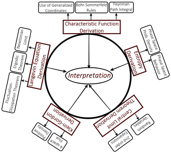
Figure 1.
The four derivations of the Schrödinger equation (the Klein-Gordon derivation is not discussed in this paper) and the main concepts linked to them. Each derivation is mathematically connected with all the others, providing a sound formal background for the interpretation.
The paper is organized as follows: in Section 2, we will present the derivation based on the construct of the characteristic function. In the third section, we will present the derivation based on the construct of Boltzmann’s entropy and mathematically show the equivalence between this derivation and the one presented in Section 2. In the fourth section, we will present the derivation based on the Central Limit Theorem and show that this derivation helps us understand some of the results presented in Section 2 and Section 3. In Section 5, we will present the derivation based on the Langevin equation and show the ergodic theorem explicitly in action, while confirming the random character of quantum mechanics. All these previous sections are based on previously published materials, now briefly organized for the presentation of the interpretation they demand. Thus, Section 6 is devoted to the interpretation that unequivocally emerges from the previous sections. In Section 7, we present two examples for the application of the interpretation: Bell’s theorem and Schrödinger’s cat. We leave our concluding remarks to Section 8.
2. The Characteristic Function Derivation
In this derivation, the statistical notion of a characteristic function plays a fundamental role. As we shall show, the following axioms allow us to derive mathematically the Schrödinger equation.
Axiom 1.
The marginal characteristic function of the phase-space probability density function , defined by
where ℏ is a universal parameter with dimensions of angular momentum, is such that it can be written as
and should be expanded to second order in the parameter .
Axiom 2.
For an isolated system, the joint phase-space probability density function related to any quantum-mechanical phenomenon obeys the Fourier-transformed Liouville equation
to second order in .
Please note that the Liouville equation appears integrated and this integral should be considered up to the second order in the parameter . This is important since this shows that the resulting probability density function in phase-space is not a solution of the complete Liouville equation, in which case it would mean that the derived equations are deterministic and, indeed, Newtonian. The details of the derivation can be found in [18] or [19]. We give only a sketch of it here.
Thus, we begin with Equation (3) and make the characteristic function appear in all terms by manipulating the integrals to obtain the equation for the characteristic function as
We now put
and use this result and the expression (2) expanded to the second order in to write
If we note, using (5) and the definition of the probability density and momentum, that
we may substitute the function (6) into Equation (4) and separate the real and imaginary parts to obtain the equations
and
which are known to be equivalent to the Schrödinger equation. In fact, if we write the probability amplitude as in (5) and substitute it into the Schrödinger equation, we obtain the two Equations (8) and (9)—essentially Bohm’s approach applied ’backwards’ (see [2]).
Of course, this expansion to the second order becomes what remains to be explained. However, we can advance, at this point only qualitatively, that it is known that when a characteristic function is truncated to the second order, there should be some relation to the Central Limit Theorem. This relation will be clarified in Section 4, as a means to explain that this truncation is, in fact, exact.
Please note that it is this truncation of the characteristic function that introduces important differences between this approach and Wigner’s definition of a probability distribution on phase space [20]. Thus, we should consider this truncation as an essential element of the approach. Note also that, at this point, we do not know the formal expression of the phase-space probability density function . This will be presented in the next section.
The averages of phase-space functions of type can be calculated simply as
once we know the formal appearance of F.
We must acknowledge the importance of being able to derive the Schrödinger equation from more basic postulates. The symbols of these postulates are already interpreted, and any interpretation that appears for the quantum-mechanical formalism must be related to the meanings of symbols that pertain to the axioms in a sort of semantic inheritance. Thus, as an example, it is easy to see that
where is the configuration-space probability density function and is the average momentum. It is easy to show that the previous expression for the average momentum, when written in terms of the wave functions, becomes
from which one defines the momentum operator.
Thus, it follows by semantic inheritance that must be a configuration-space probability amplitude. This is something to praise, if one remembers how difficult it was to arrive at this conclusion in the decade of 1920, with all the discussions between Schrödinger and Bohr, which finally ended with Born’s interpretation [21]. Moreover, at this point of the derivations, Equation (3) means that quantum mechanics is a theory related to ensembles—this will be expanded, with qualifications, to single systems when we present the derivation based on Langevin equations, in Section 5. Please note that the derivation does not allow one to talk about observers, reductions, branches, stochastic support, etc. Thus, we should not be allowed to introduce these ontological entities, except by brute force.
Of course, the point now is on the reliability of the derivation. This derivation has some formal consequences that help us with that, and we briefly present them in what follows.
2.1. Derivation in Generalized Coordinates
One of the main tests for an axiomatic approach is its ability to “survive” extensions of it. For example, and at the most basic level, the derivation made in the previous section is easily generalized to any dimensions. We should only write the axioms in the desired dimension to arrive at the Schrödinger equation written in this chosen dimension.
Besides that, the last developments allow us to make the derivation of the Schrödinger equation in any coordinate system, instead of making the quantization in Cartesian coordinates and then changing to the desired coordinate system. Of course, a theory cannot depend on the arbitrary choice of the coordinate system. However, quantum mechanics does not have a process to make quantization directly from a Hamiltonian written in any coordinate system [22,23,24]. The situation is shown in Figure 2.
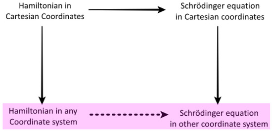
Figure 2.
The usual approach to quantum mechanics does not furnish a general method to quantize directly in any coordinate system. The present axiomatic approach allows for that by simply writing the axioms in the desired coordinate system. It fulfills the process represented by the dashed line, without which the theory would depend on the (arbitrary) choice of a particular (Cartesian) coordinate system.
For an axiomatic approach, this is not a matter of mannerism. If we want to find a reliable derivation, it must pass this generalization test and shows itself capable of finding the Schrödinger equation in any coordinate system, as long as we write the axioms in the desired system. This result may be shown, and the calculations for the spherical coordinate system may be found in [18]. It should be noted that the calculations, although of a simple algebraic type, are extremely long. The lengthy calculations are presented in a file using algebraic computation, which is referred to in the Supplementary Materials Section. This result should increase our confidence in the present derivation using the characteristic function.
2.2. The Role of the Bohr-Sommerfeld Rules
The Bohr-Sommerfeld rules are usually assumed to be part of the “old” quantum theory [25]. The present derivation shows that this is not the case. In fact, the Bohr-Sommerfeld rules are an important part of the overall formal structure of the theory.
This result comes easily from the fact that the characteristic function is the Fourier transform of a product of functions. The convolution theorem implies the Bohr-Sommerfeld rules, as mathematically shown in [18]. Moreover, as shown in that paper, the Bohr-Sommerfeld rules come with an integer or a half-integral number. The absence of this last result is another point stressed in the literature to rule out the Bohr-Sommerfeld rules as adequate to the quantum formal apparatus (see [25], p. 48). In the mathematical derivation process of these rules [18], one is informed that they can be strictly applied only in situations where one has some symmetry in the physical system. Thus, one should not expect them to strictly apply to atoms with two or more electrons, which is another criticism made in the literature (see [25], p. 48).
These rules can be used to interpret, in corpuscular terms, “wave-like” phenomena [26,27,28], such as the double-slit interferometry—something that would reveal itself important in the overall interpretation of quantum mechanics, to be presented in Section 6.
2.3. Connection with Feynman Path Integrals
It is easy to show [18] that the present derivation is equivalent to Feynman’s path-integral approach [29]. To do this, we stress that
and we put . This means that represents the velocity taken over the same trajectory, since in general we would have
where is the separation between two distinct trajectories (which we make equal to zero). We must have
which is an expression for the Principle of Least Action. We may now use
where is the classical Lagrangian function and E is the energy (supposed constant) of the system under consideration. We end up with the expression (see [18])
where is the Jacobian of the transformation . From this last expression, we continue on the same steps as Feynman to arrive at the Schrödinger equation.
It is thus easy to see from (14) that in our approach is in Feynman’s, which is a parameter that he uses to expand his results to second order. Thus, the two approaches are equivalent, one being performed upon the configuration-space, the other being performed upon phase-space. This is another point in favor of the reliability of the present derivation.
With this last result on the equivalence with Feynman’s path-integral approach, we may say that in our approach, we are summing over phase-space trajectories. This resembles the stochastic construct of “realizations” of random movements. However, we must not rush in interpreting this in this manner, since there is no trace of randomness in the formal structure of the derivation. To be capable of restraining from these kinds of hurried conclusions is our main argument against other derivations, based on other semantic constructs. “Realizations” and “stochastic behavior” must be introduced only after the formalism is further developed to support their inclusion in the interpretation. We do that in the following sections.
3. The Entropy Derivation
The formal equivalence between our approach and Feynman’s means that one may derive the Schrödinger equation following different formal paths, with the introduction of different constructs (or axioms, when it is the case). If this is the case, these other derivations can give us a clearer picture of the theory with respect to the formal constructs introduced. It is not the case that interpretation constructs, without the correlating syntactic symbolic element, would be introduced—we are avoiding exactly this kind of approach. This is why it is so important to show that one derivation is formally equivalent to all the others. Thus, new formal constructs can come to our help to give us a better grasp of what the theory is talking about after we show that these constructs indeed are rooted in the theory’s formalism.
In this section, we continue to use the axiomatic approach and use the concept of Boltzmann entropy to mathematically derive the Schrödinger equation. However, note that we will use different axioms, which implies that the present derivation is completely independent of the one presented in the previous section. This is particularly interesting because it allows us to compare and interrelate the axioms, thereby making the correlation between the whole theory under scrutiny. We begin with the new axioms:
Axiom 3.
For an isolated system, the joint phase-space probability density function related to any quantum-mechanical phenomenon obeys the first two momentum-integrated Liouville equations as
Axiom 4.
The product of the variances of the momenta and the positions of a physical process, calculated at each point q of the configuration space, must satisfy (see [30] for a rationale for this axiom)
Equation (17) means that we pick a strip or fiber in phase space in the interval (since we work with probability densities). Then must be interpreted as the variance of the momentum variable calculated on this fiber at the instant of time t. Equivalently, in this same fiber, represents the variance of the variable q at the instant of time t. Thus, Equation (17) means that, on any fiber labeled with q, the product of variances in variables p and q must be equal to . This is a very stringent constraint imposed on the phase-space probability density function.
Moreover, the two equations in (16) do not mean that the classical Liouville equation should be satisfied by the probability density function , which would cause quantum mechanics to collapse into Newtonian mechanics. We impose only that the first two statistical averages there represented, integrated in the variable p (that is, over a fiber), must be zero. These equations mean conservation of probability and conservation of momentum in the configuration space.
The present derivation is less direct than that using the characteristic function (see [26,31] for more details). We first introduce the two definitions [32]:
where the first represents the usual way in which one calculates the marginal probability density function on the variable q, while the second represents the calculation of the average momentum defined in the configuration space (not to be confused with the dynamical variable p, without the explicit dependency on q).
To proceed with the derivation, one must expand the Liouville equation and integrate it in the variable p to find, using (18), the continuity equation
which is the first equation to be obtained.
To obtain the second equation (see the previous section), one must multiply the Liouville equation by p and integrate it into this variable to obtain the equation
where represents the second statistical momentum moment of the variable p and is defined by
We thus define the variance of the momentum variable over some fiber labeled by q as
Now, consider the entropy defined in the configuration space in such a way that the equal a priori probability postulate grants us that (see [33], pp. 290, 509)
where is Boltzmann’s constant—this is why we are presenting this derivation in more detail, since we want to show at which point Boltzmann’s entropy comes into play. We now disturb the probability density function in the vicinity of by writing in such a way that we have
This means that the disturbed , when considered up to the second order, is a Gaussian function. Please note that continues to depend on the variable q, showing that the amount of disturbance is an independent variable with respect to q. The final disturbed function gives the characteristic function, since the averages and variances that come from it are those that come from the underlying characteristic function (see [34], p. 172 or [33], pp. 288–291; see also Section 3.1 in what follows). Please note that we develop the last expression to second order in (which begins to show the deep connection with the derivation made in the previous section).
Thus, it is obvious that
where we put
We thus have that
but we would like to have an expression for
Generally speaking, for a general physical theory, the dispersions in variables q and p are independent of each other. However, Axiom 4 of the present section makes them depend upon each other and introduces the main feature of quantum mechanics; in what follows, we will show that this expression gives the usual Heisenberg dispersion relations.
Indeed, the content of the second axiom (and quantum mechanics) allows us to write
and thus
Substituting [31] this expression into (20) and writing, as in the derivation of the previous section,
we find the equation
Equations (19) and (25) were already shown in the previous section to be equivalent to the Schrödinger equation
if we write as presented in (24). This ends our derivation.
3.1. Equivalence to the Characteristic Function Derivation
Now, it is important to show that both derivations give the same interpretation of the theory, but using different constructs (characteristic function and Boltzmann entropy). This should also improve our confidence in the derivation processes (if one is not yet convinced of their adequacy, see Figure 1).
To do this, we take the definition of the characteristic function of the last section and expand the exponential of the Fourier integral nucleus in a power series to write the characteristic function, to second order in , as
and, using (18) and (21), we rewrite it as
We now substitute (26) into the equation satisfied by the characteristic function (see previous section) and take the real and imaginary parts to find Equations (19) and (20). This shows that both mathematical derivations are formally equivalent.
As we said, the proof of the equivalence between the two derivations is of utmost importance for our objectives. Indeed, the two derivations use different constructs (characteristic function and Boltzmann entropy). However, both are introduced from axioms that are already interpreted with respect to all their symbols and have been proved to be mathematically equivalent. Thus, by semantic inheritance, we can expand our understanding of the quantum-mechanical formalism, which we do in the following sections.
3.2. Heisenberg Dispersion Relations
From the relation (17), with an equal sign for each point of the configuration space, we can mathematically derive Heisenberg’s dispersion relations (see, for example, [30] or [31]). Indeed, if we begin with
and use
then
with and as implied. If we integrate the first integral by parts, we obtain
By manipulating this equality in a straightforward manner (see [31], for details), we obtain
The last result is important. Please note that the equality sign for each fiber on the phase space labeled with q blocks any interpretation based on some kind of measurement theory or an interpretation of a subjective type. All quantum-mechanical systems have the same property, which is an objective property of them. Heisenberg relations inherits this feature from the axiom. Even if we look at Heisenberg’s dispersion relations (not uncertainty relations) with a greater or equal sign, we must acknowledge that this sign is there only because we are abstracting from the particular state. Indeed, once the (pure) state is fixed, one must have an equality sign. For example, in the case of the harmonic oscillator, we have the equality , where is the frequency of the oscillator and n gives the state. This means, again, that this relation regards an objective feature of the physical system (in this case, the harmonic oscillator). Indeed, it is quite difficult to argue how two different observers, measuring with different apparatuses, would obtain exactly the same result for the product of the dispersions; on the other hand, to say that this relation is an abstraction of the concrete experimental context is just to affirm that it should be considered an objective property.
The question, of course, is: Where did these dispersions come from? They come from the kind of separation we make in the physical system, by looking at the particle subsystem in detail, while assuming only a fixed expression for the field subsystem that furnishes the potential , something that announces the role of fluctuations, without making them explicit. At this point, just as an example, it is instructive to watch any simulation of a wave packet colliding with a potential barrier. When the wave packet enters the region of , it begins to deform, but the potential barrier keeps its form as if nothing were happening, despite the obvious fact that a physical interaction begins (see [35], pp. 106–107). This can only happen if we are looking at quantum mechanics, as given by the Schrödinger equation, as a mean-field theory in which we keep our attention on the particle subsystem while assuming only an average behavior for the field subsystem.
This resembles the Brownian movement situation, roughly speaking. In the Brownian movement, we are interested in the (large) pollen particle and consider the shocks that come from the colloidal (much smaller particles) in average terms. In this sense, quantum mechanics is established in the canonical ensemble picture, the field playing the role of a thermal reservoir. We formally and explicitly address this feature in Section 5, when we present the derivation based on the Langevin equation.
3.3. Positive Phase-Space Probability Density Function
We may invert the Fourier transform that defines the characteristic function to find
where we already used
and we put the variance density in p as
If we note that , the expression (27) tells us that the phase-space probability distribution function for any phenomenon of quantum mechanics is given, at each fiber of the configuration-space labeled by q, as a Gaussian function with average momentum given by and statistical variance given by .
A more detailed exposition can be found in [31], where we present the harmonic oscillator and the hydrogen atom examples. If we consider, for example, the state of the hydrogen atom, we can present an example of a phase-space probability density function as
Calculating the average energies, momenta, and other properties of this state using gives all theoretical quantum results [31], as for any other state. These calculations are presented in an algebraic computation program, which is referred to in the Supplementary Materials Section.
However, at this point, we recall that we have truncated the characteristic function (to the second order in ). The question then is whether we can make such an inversion of the Fourier transform (when we integrate from 0 to ∞). It seems that if we have a truncation, the results obtained would be approximate, in the best case. However, all results are exact in the examples cited before. In Section 4, we will show that the expansions to second order so far adopted (and Feynman’s too) are exact, when we present the Central Limit Theorem and its role regarding quantum mechanics.
3.4. Phase-Space Behavior
The axioms do not assume that the phase-space probability density function satisfies the Liouville equation, but only to the second order in the parameter . However, it is instructive to consider the application of the Liouville operator to the quantum phase-space probability density.
In Figure 3, we plot the function
for of the harmonic oscillator. We divided the Liouville operator applied to by itself to avoid the Gaussian exponential decay of the phase-space probability density function, which would cause the result to go to zero.
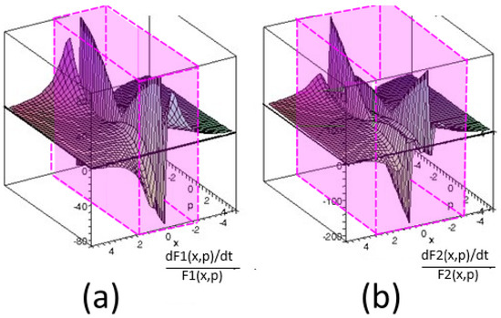
Figure 3.
Behavior of the functions for and in panels (a) and (b), respectively. The images show the strong variations of the phase-space density near the fibers at which the fluctuations diverge (in magenta), while they satisfy Liouville’s equation far from these divergence fibers.
In Figure 3, it becomes apparent that the Liouville equation is satisfied almost everywhere, except in the fibers where the probability density functions of the phase space have divergences. On these fibers, the result of the application of the Liouville operator to the probability density function strongly oscillates. The two integrals in the first axiom, Equation (16), remove these behaviors by averaging over the fiber and give zero as a result. These results, together with the calculations related to the harmonic oscillator in general, are made using algebraic computation in a file presented in the Supplementary Materials Section.
4. The Central Limit Theorem
This section is of utmost importance because it gives consistency to the last two derivations with respect to the expansion to the second order in . Indeed, as we have noted in Section 2, we used the characteristic function, developed to the second order in the parameter . At that point, since we did not present a reason why this expansion should terminate at the second order, we have no option but to assume that this was a truncation of the characteristic function and thus an approximation.
However, in Section 3, we inverted the Fourier transform that defines the characteristic function and thus integrated the variable within the interval . The only way we can perform the inversion is if the characteristic function expanded to second order is not a truncation, but its very exact expression.
This happens, as is well known, when the system obeys some version of the Central Limit Theorem (CLT). We therefore expect that the CLT is deeply rooted in the quantum formalism.
We will show this in this section. Please note that the CLT is related to sums of random variables, and this will bring us closer to our objective, i.e., to show, mathematically and explicitly, that quantum mechanics has a stochastic support—and to find the equation that gives this support.
4.1. Phase-Space Sampling and Sums of Random Variables
It is easy to see from the definition of the characteristic function that momentum is the random variable with which to cope. One may think of a particle filling the phase space by moving around, assuming values of phase-space points that are random (q being random because of p—see next section). Let us turn to discrete variables (see the next section). Of course, each infinitesimal region of size , centered in in phase space, will have a probability of being filled, which may vary as the system evolves in time (see Figure 4).
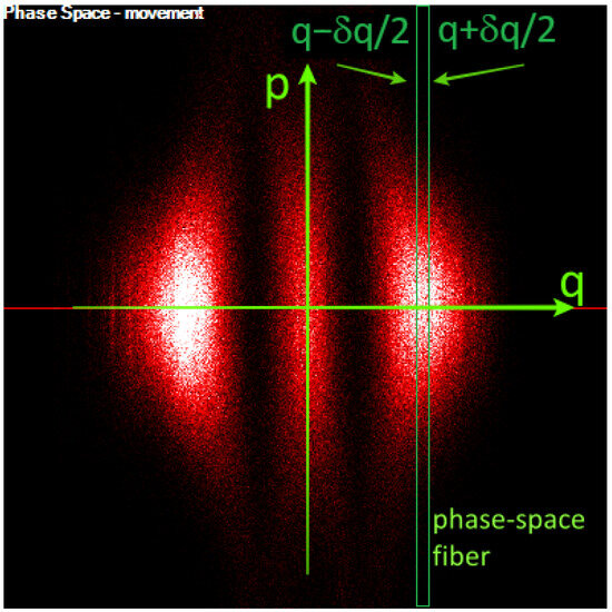
Figure 4.
Sampling over the phase space related to the marginal characteristic function formulation. The image is related to the dynamics of a harmonic oscillator in state after some time filling the phase space—after 1,000,000 points in a simulation done by the authors (see next section on the Langevin equation for quantum mechanics). A phase-space fiber at the point q is presented.
Thus, the mathematical expression for the marginal characteristic function means that, at any instant t, a sampling of the whole phase space is carried out by fixing the variables and t and sampling over the respective fiber of this space (in which p varies from ).
Of course, since we are looking at a probability density, this sampling must be taken in the interval , i.e., each sampling is performed in phase space within a fiber of width that is parallel to the momentum axis. This means that can be written as , where is the conditional probability density that one obtains , given that has occurred. Since we are within a fiber of size , one must have different outcomes of within it, with different probabilities densities , but, assuming and are independent, the probability density ( at the center of the fiber k) will be given by
Our interest lies in the variable
where are the random momentum variables when q is within the fiber indexed by , its center, and N is a number that we will make go to infinity to obtain the variable P.
Assuming all these characterizations, the derivation of the CLT for quantum mechanics is straightforward, as the reader may verify in [36,37] and will be briefly presented in what follows.
Of course, in any derivation process of the CLT, one never finds any physical equations related to quantum mechanics or any other physical theory. The derivation is simply a matter of statistical calculations using the Levy approach [38].
Indeed, what makes this calculation adequate for quantum mechanics is the assumption about phase-space sampling and the way we write the marginal characteristic function. This is extremely important: it is because we write the marginal characteristic function as the product
and expanded it to second order that we have the link between the quantum formalism and the CLT—see next subsection. This is shown explicitly in [36], in Equations (30)–(33) of that paper.
Thus, if the CLT applies, we end with the probability density function, defined in phase space, for any quantum problem as
where the average and variance , defined on the fiber q, are given by
and
now written in terms of the characteristic function only, as one can find, for instance, in [39].
This last comment brings us to the main objective of making this connection. We are now in a position to understand the and expansions to second order, and we address this point in the next subsection.
4.2. Meaning of Second-Order Expansion
We then present quite briefly the Central Limit Theorem and its proof, while pinpointing some important aspects regarding its relation to the characteristic function derivation.
Theorem 1.
Consider, for a given fiber centered on q in the configuration space, a sequence of independent random variables with and . If we put then, under very general conditions, the reduced variable
where
has approximately a Gaussian distribution with and . Thus, if is the probability distribution function of the random variable , for each fiber centered in q, whose probability density in the configuration space is , then we have
where
and
Proof.
(We will demonstrate the theorem only for situations in which the are all equal, and so are all the . However, the theorem has a much wider applicability [38]). Under these assumptions, we have and (note that this means that must go to zero with as we make , the same being valid for m. Consider now the probability of being in some interval after n steps, each within , with probability
where we assume that all are identical and are in the interval ). We assume that , since is the probability of being in the vicinity of and is the conditional probability of being in the vicinity of assuming that the system is in the vicinity of .
In this case, we obtain, as we have already noted,
and, as a consequence, it is possible to obtain our probability function as
We then use [33]
and
Now, if instead of working with , we use the rescaled random variable , such that
(note that refers to each ), then the properties of the Fourier transform give us
This last result means that the rescaled characteristic function related to the variable P must be given by
since we are considering the independent variables, a demand of the Central Limit Theorem. In fact, in this case, the characteristic function of their sum is just the product of the characteristic functions of each (actually, this is one of the most important features of the characteristic functions).
Thus,
and we can develop in the Maclaurin series as
where all the derivatives are with respect to and , the remainder of the expansion is a complicated expression of these quantities and powers of n [39] in such a manner that . Since the definition of implies that
we may write
and, thus,
Please note that is a finite quantity, while and are infinitesimal, in the sense that they go to zero as when . However, note that there is a factor n multiplying the logarithm in the last expression. This means that we will have to search for the expanded expression in the logarithm.
Since we want results for , we develop the logarithm in power series to find
Please note that the first two terms in the brackets cancel out, and we end up with
where depends on n as some inverse power law of type with [39]. Thus, if we take the limit , we obtain
which, upon inversion, gives the Gaussian probability function (
which is the result we were willing to show. □
It is important to note that we have two variables and P (see the previous subsection), so that for each of them there are variables and . The variable is connected to the probability densities of individual results and can be made infinitesimal. However, the probability that comes from the sum in (30) is defined as
giving the relation between the infinitesimal and finite characteristic functions as
where in such a way that the finite case is related to , with , while . Thus, despite being infinitesimal, is finite, and this last variable is being integrated in the inversion of the Fourier transform.
We can compare the result (50) with our expansion of the characteristic function to see their equivalence. Indeed, we have to second order (see (6))
If we now expand this result in terms of , we obtain
The second term is easily recognized as the momentum average . The third is simply , and the fourth is
which is just , according to the results of the previous section, such that we have exactly the same expression as shown in (50).
These results allow us to rewrite the axioms of the approach as
Axiom 5.
The characteristic function of the random variable can be written (in the limit ) as the product
for any quantum system, and quantum mechanics refers to the universality class defined by the Central Limit Theorem.
Axiom 6.
For an isolated system, the joint phase-space probability density function related to any quantum-mechanical phenomenon obeys the Fourier-transformed Liouville equation
to second order in .
Please note that the first axiom already implies that the marginal characteristic function should be developed up to the second order in —these two statements are equivalent.
At this point, the two derivations presented in sections two and three were shown to be formally adequate. Now, and only now, we can say that quantum mechanics is a theory with stochastic support. Moreover, we know that this stochastic behavior comes from the separation of the field and particle subsystems, in which the field subsystem plays the role of a heat reservoir, and the whole theory (based on the Schrödinger equation) is a mean-field theory, or it is of the type of a canonical ensemble in the terms of statistical mechanics. This is a completely objective source for the fluctuations.
Despite the fact that the CLT has given us all the previously mentioned understanding, it uses random variables whose values come from some equation yet to be determined—the Schrödinger equation cannot do that, of course, since it is already the result of the washing out of the random behavior. We present this equation in the next section.
5. The Langevin Equations of Quantum Mechanics
Approaches proposing stochastic support for quantum mechanics flourished in the early 1950s [40] and had received many different formats of presentation [5,41,42,43,44,45,46,47,48]. It is still a proficuous field of investigation, but the interpretation they propose, in general, does not take part in the mainstream of the interpretations of quantum mechanics.
Our objective is to find an equation that provides concrete values for the random variables that appeared in the CLT, i.e., the concrete values of the stochastic realizations of some quantum-mechanical system. This means that we are searching for a true stochastic equation with which we can make actual simulations, for instance. An equation, for example, of the Langevin type. All the stochastic derivations of the Schrödinger equation do not provide such an equation, but some sort of Bohm’s equation, which is equivalent to the Schrödinger equation (as we did up to this point). Thus, these derivations are at the same level of description as those we advanced in the previous sections. We will explicitly show that in the next Section 5.1.
In fact, as we shall show, these derivations are of great importance, since they are able to show the reason why the random variables do not appear in some concrete random variable equation, such as one of Langevin type. This provides an argument for our own interpretation that the Schrödinger equation is a sort of mean-field approach.
We then must try to find an equation that concretely deals with random variables and that connects these variables to the momenta of the physical system and still recovers all the behavior of any quantum-mechanical system. This means that this equation should reduce to the Schrödinger equation when averages are taken. As we shall show, this equation is the Langevin equation, modeled to give the appropriate results of the usual quantum theory in the appropriate limit.
In what follows, we present one usual derivation of the Schrödinger equation from a stochastic rationale and show the averaging process we were talking about. We then present the Langevin equation of quantum mechanics.
5.1. Stochastic Average Derivation
Many stochastic derivations of the Schrödinger equation can be found in the literature [6,7]. However, in this section, we only sketch the stochastic derivation of de la Peña [7,49], which makes the stochastic variables and their properties explicit. The interested reader may find all the details in [50]. We will adapt de la Peña’s derivation to one dimension as a means to simplify it. This will make the comparison to what we have done in Section 2 immediate.
Thus, let us begin by assuming that the velocity c of the particle is the sum of a systematic or current velocity v and a stochastic component u
De la Peña, thus, introduces a time-inversion operator that can distinguish between systematic and stochastic velocities. He manipulates the equations of his approach using this operator to derive the Schrödinger equation.
If we are trying to present how some quantities f vary with time, i.e., , we need to assume situations in which the position q changes with respect to time
where we assume to be very small (compare with Feynman’s path-integral approach). Suppose now that is any smooth function of q and t; we can write
Of course, this change becomes a distribution with respect to the variable .
We now take the average of the above expression (average values with respect to the distributions). It is at this point that the concrete random behavior of the approach is lost, and we are left with average results (or a mean-field theory); note that this means that Bohm’s approach must be considered in the same fashion, if our calculations end up giving Bohm’s equation. Thus, we find
where the parameters represent the limits of the first- and second-order moments of the distribution f with respect to the values of the variable , divided by . We identify c with the components of the velocity c. Again, this means that all the dependence of the equation on is now inserted into the coefficients , which are the results of the averaging process. Note also that in the limit when . Peña calls the forward derivative operator.
Using the time-inversion operator, de la Peña introduces the backward derivative operator, and, using both, he obtains, after some lengthy manipulations, the two equations
where is the force. These are our primary equations.
Equation (65) can be written as
This system of equations can be shown to be equivalent to the Schrödinger equation. In fact, when imposing certain conditions on the constant terms appearing in the previous equation, we can recover the Schrödinger equation. Furthermore, these conditions on the constants and their relations to the velocities (systematic and stochastic) give the connection between the present approach and the characteristic function derivation of the Schrödinger equation, shown in Section 2.
Indeed, looking at the equations that lead to the Schrödinger equation in Section 2, we write
where and are real dimensionless functions of q and t, and put , , , to get
In de la Peña’s derivation, it is not clear what it means to make this choice for the constants, but the resulting equation is the same as that we obtained in sections two and three and is thus equivalent to the Schrödinger equation, as already mentioned.
The expressions (67) provide the explicit connection to our derivation based on the entropy construct, since we can rewrite the stochastic velocity u in terms of the entropy as
where and . Moreover, this equation is related to the content of the fluctuation-dissipation theorem (see [33], pp. 594–597). Equation (67) give the statistical character of and , but conceal their concrete fluctuation behavior. To address this fluctuation behavior, we must take a step further.
5.2. Stochastic Langevin Derivation
The Central Limit Theorem was proved without knowing which equation would furnish the sums of random variables that the theorem assumes, and the stochastic results obtained so far cannot provide such sums. In this section, we will find a true stochastic equation for quantum mechanics in the form of a Langevin equation [50].
Thus, let us begin with a two-dimensional system (phase space of a system with one degree of freedom) for which our proposed Langevin equations are given by
The rationale for presenting the equation in this form is that we should expect some departing from Newton’s equations, but given solely in terms of the elements that pertain to the framework of a Langevin equation, i.e., the fluctuation and dissipation terms. Please note that all these terms provide a picture of the way the field subsystem interacts with the corpuscular one. Indeed, for the example of the electromagnetic field, and assuming the instance of virtual photons, we can say that the first and last terms on the right-hand side of the first equation show how the force field changes from its mean value when some virtual photons are exchanged between the corpuscular and the field subsystems. The functional appearance of these fluctuations, given by , is left as a way to adequate this proposal to furnish the correct quantum-mechanical results. We also assume, in the context of a Langevin equation, that
Since we consider each fiber in the phase space defined by some value of the variable q, we will keep q constant and work only with the first equation. This equation in (70) may be solved by discretizing the time parameter to find
such that
Thus, the same considerations about the way we make our sampling of the phase space advanced in the derivation of the Central Limit Theorem also apply here. In this sampling, we are not iterating on the variable q because we are looking for the momentum probability distribution for each point q in the configuration space. Thus, for each such point q, is a random variable that we can consider using traditional statistical methods.
In the ensemble approach of a one-particle system, for instance, we let the particle in each one-particle system begin at any point in the phase space and, after some definite time given by , we make our statistics over the fiber using the characteristic function given in (78), by collecting the momentum and position in each system and building from them a statistical frequency diagram. In the single-system approach for a one-particle system, for instance, we let the particle fill the phase space and collect, at each small step , its position and momentum to make from them a statistical frequency diagram. Please note that the ergodic theorem says that these two sampling methods must give the same result.
Now, iterating (72) and putting , for simplicity, we find, for the nth iteration (see [50,51] for more details on the calculations in this section)
and using Equation (72), we have, for the first two iterations,
and, in general,
If we put , for simplicity, we obtain
Thus, is the sum of independent random variables, which we defined in the previous section as , while is equivalent to the variable , both defined in Equation (30). This makes a bridge between this approach and the one based on the Central Limit Theorem.
We can connect these two approaches with that of the characteristic function by writing this function for (the uppercase will be related to the whole sum of random variables, up to n; when we take , we will drop the index n)
where we note that because the functions depend on q, we must have the same dependence for the characteristic function . In fact, the averaging process represented in (78) is explicitly given by
where is the probability density function related to each .
Thus, since we write as (79) with ,
where we are supposing that all variables have the same underlying joint probability distribution function (see the derivation of the Central Limit Theorem). Now, (78) can be written as
which results in (see the discussions in Section 4.1)
since the ’s are all independent random variables—note that the averages are now taken with respect to and the characteristic function (for each random variable of the sum) is such that .
Now, using (77), we can write, for example,
Using (74), we find
and higher-order expressions.
The variance of the random variable becomes
and, thus (up to second order—we justify that in what follows),
Please note that this is, essentially, the expression of Equation (6) found in Section 2, now explicitly presented in terms of random variables.
Thus, we obtain, for the total characteristic function,
where
and
where is called the average momentum; note that this nomenclature is appropriate since is a force depending only on the random variable q and is a time, and thus has the dimension of an average momentum (an impulse), so it could be explicitly written as
and is usually called (in non-equilibrium kinetic theory) the macroscopic average momentum [32] (as introduced in Section 3).
The expression (87) automatically implies, by inversion of the Fourier transform, that
where we have already normalized the density . Now we may take the limit , , such that , to find (note that the index n must now be dropped)
where
which are both geometric progressions. Using , we obtain
Adding the geometric progressions in (93) to n, and taking , we obtain [50]
and asymptotically, ,
Thus, we end with the asymptotic distribution,
which is the joint probability distribution related to the Langevin system of Equation (70).
For the third-order statistical moment, as given by (83) (and higher ones), we obtain results such as
which goes to zero as . This is another way, related to the Central Limit Theorem, to justify our assumption of a second-order development of the characteristic function. All our expansions up to the second order in are not approximations. This is the very expression of the CLT, rephrased using the Langevin equation and the justification for the derivation using the characteristic function. Furthermore, this shows the deep relations between all the derivation processes already presented.
The second equation in (70) makes the overall span of the whole phase space, since it is connected by the probability density function for each fiber and allows the sampling to be over all points in the phase space. The probability densities, in fact, the probability amplitudes, are obtained by means of the Schrödinger equation, which, in the perspective of this approach, has exactly this role.
The result (96) shows that, for each point q of the configuration space, the momentum probability distribution is of Gaussian type, exactly as in (32) coming from the Central Limit Theorem.
We have already connected the present approach to the derivations of the previous sections. However, in order to make it possible to make actual simulations, we must find the formal structure of the fluctuation term.
Since the probability density functions in phase space must be equal, beyond being both Gaussian, we must compare the result (96) with (32) for any quantum system. This implies making the identification
where both and come from the solution of the Schrödinger equation with
Because of these identifications, the fluctuation term in the first Langevin equation representing the momentum fluctuations becomes
and enters into the general Langevin equations as a true random force, due to . Thus, the relation with the Bohmian “quantum potential” becomes clear: Bohm’s equation is an equation for average values (such as ) and the “quantum potential” does not appear as a true random force, but only an averaged one.
In the next sections, we present some results obtained by making simulations of the Langevin equations. Two physical systems are considered: the one-dimensional harmonic oscillator and the one-dimensional Morse potential. We also show, for the harmonic oscillator example, the relation between the results of the simulation of the Langevin equations (70) and Bohm’s equation [49,50]. In the Supplementary Materials Section, we present a small algebraic computation program that simulates the Langevin equation for the harmonic oscillator.
5.2.1. The Harmonic Oscillator
The potential (we put )
gives the non-normalized probability amplitudes
where are the Hermite polynomials. Some results for the probability density function on the configuration space obtained with the simulations are shown in Figure 5 as dots. As can be seen from this figure, they are very good compared to the theoretical results obtained from the solution of the Schrödinger equation. These simulations were performed considering a single particle system that moves randomly in phase-space. One can also make ensemble simulation of these equations to obtain equivalent results (see the section below on the ergodic theorem).
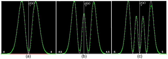
Figure 5.
The fitting of three probability density functions in configuration space for the states in panels (a), (b), and (c), respectively, of the harmonic oscillator system represented as green dots. The continuous curve is the theoretical result coming from the solution of the Schrödinger equation.
As a way to compare the results of this section and those of Bohmian mechanics, we plot the constant-energy curves coming from Bohm’s potential (for some values of the total energy), the equal probability curves coming from the phase-space probability density function, and the filling of the phase space coming from the simulation of the dynamical Langevin equations. The result is shown in Figure 6 for the first two excited states of the harmonic oscillator.
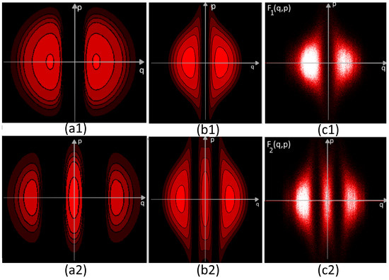
Figure 6.
Bohm’s trajectory for constant energy (a), equal probability curves of the phase-space probability density function (b), and the filling of the phase space (c) made by simulating the corresponding Langevin equations. The states are given by the quantum numbers: 1 (above) and 2 (below).
5.2.2. The Morse Oscillator
The potential function is
such that
where and are the Laguerre associated functions. We made our single system simulations for and for the quantum numbers .
The probability density functions in the configuration space (above) and the corresponding probability density functions in the phase space (below) are shown in Figure 7 and show a very good fit to the theoretical ones.
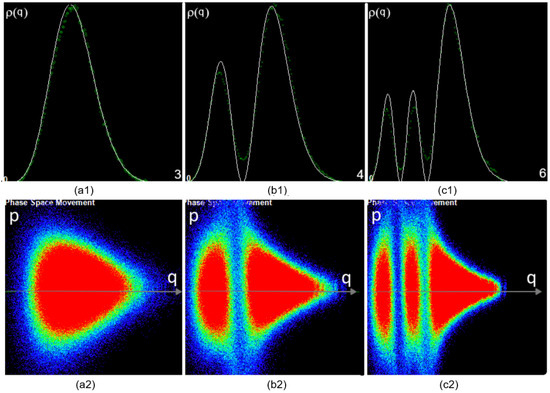
Figure 7.
Above we show the probability density functions in configuration space for states in panels (a1), (b1), and (c1), respectively, of the Morse oscillator with . The continuous lines are the theoretical curves coming from the solution of the Schrödinger equation. Below, we show the corresponding phase-space filling, in panels (a2–c2) for the same states.
With the Langevin equation defined for any dimension in phase space, one can simulate the stochastic behavior of whatever physical system of interest. It is possible to obtain much information from these simulations. Some of them are presented as follows:
- The ergodic theorem: we mentioned in a previous section that we can make simulations of the ensemble type or the single-system type using the Langevin equation, adequate for a specific physical system. In fact, the ensemble-type simulation is always possible, but single-system-type simulations depend on the experimental setup being considered. For instance, it is possible to make both types of stochastic simulations for the isolated atom, molecule, or solid, but it is impossible to make a single system-type simulation for the double-slit experiment, since each particle sent to the slit is absorbed by the detectors, and one has to send another particle (another one-particle system) in a necessary ensemble-type simulation. We will show that this implies very important interpretive consequences in Section 6. However, at this point, it is important to stress that the results obtained by ensemble-type or single-system-type simulations, for situations where the latter is possible, always give the same result, showing that the assumption of the ergodic theorem in the context of quantum mechanics is adequate for these situations [50]. We present the results for the first three states of the harmonic oscillator in Figure 8.
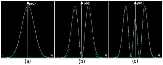 Figure 8. The results of the stochastic simulations in the ensemble picture using the Langevin equations for the quantum-mechanical harmonic oscillator. States are shown in panels (a), (b) and (c), respectively. Lines refer to the theoretical results, and dots refer to the simulations. The stochastic simulations were made using 10,000 realizations with 1200 points in each of them.
 - The fluctuation-dissipation theorem: the Langevin equation differs from the Newtonian equation by introducing a dissipation and a fluctuation term. It is possible to show, using simulations of the Langevin equation, that one has the quantum-mechanical version of the fluctuation-dissipation theorem of statistical physics.
- The Newtonian limit: using single-system simulations it is possible to show that, by variation of the parameter (see the previous section), we can go continuously from classical mechanics (when ) to quantum mechanics, when one obtains the quantum-mechanical probability density for some non-zero value of this parameter that depends on the actual physical system being considered. This is shown in Figure 9.
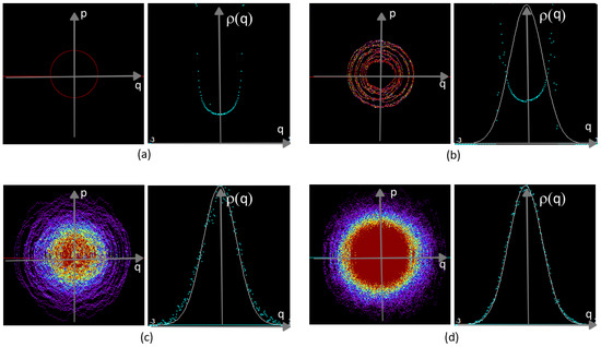 Figure 9. Simulations of the harmonic oscillator for four values of the parameter : (a) 63,000 (Newtonian picture); (b) 80,000; (c) 120,000; (d) 500,000 (quantum-mechanical result). The values of are smaller for small values of to make the integration of the trajectories more precise, and we use 500,000 points in (d) to show the “exact” situation.
With all these results at hand, we are prepared to present in the next section a panoramic view of a new stochastic interpretation of quantum mechanics.
6. A New Stochastic Interpretation
We can now, with the certainty brought by the mainly syntactical results, put forward a number of conclusions about the interpretation of quantum mechanics. In this paper, we will present the most important ones, without trying to be exhaustive. We do that in the following list with only ten possible conclusions.
- the structure of the theory: exactly as with classical mechanics, quantum mechanics relies upon two equations. The first equation represents the statistical behavior of ensembles (we return to this point later) and is the Schrödinger equation; the second equation represents the individual behavior of the constituents of the ensembles and is the Langevin equation already presented. This comes clearly from the first postulate of the first and second axiomatic derivations, for the Schrödinger equation, and also comes from the Langevin equation derivation, for individual constituents. The stochastic nature of the quantum movement of the constituents poses important differences from the classical case. Indeed, if we keep in the classical case with the same initial conditions for the constituents of the ensemble, we come out with a probability distribution function of the type , where and give the Newtonian deterministic trajectory on phase space, and is the Dirac delta distribution. In the quantum-mechanical case, which is not deterministic, and for the stationary cases, we can begin with the same initial conditions for each constituent of the ensemble and obtain the overall correct probability density function, since we are no longer restricted to a trajectory, but to realizations. This makes the Schrödinger and Langevin equations give, in the long run (stationary situation), equivalent results, but the Langevin equation can give transient behaviors that are not within the Schrödinger equation’s reach. Besides that, the Langevin equation introduces a crucial difference between nature and behavior that we address in the following item;
- on nature and behavior: the connection between the two levels of the quantum-mechanical description, individual and ensemble, mentioned in the previous item, leaves no doubt about the fact that quantum mechanics is related to particles randomly moving in phase-space. These particles, when moving this way, fill the phase-space so as to give the correct phase-space and configuration-space probability distribution functions, the latter coming directly from the Schrödinger equation. Thus, we are left with two different levels of analysis: the level regarding the individual constituents of the ensembles, which are particles, and the result of the behavior of these constituents as time elapses, which are given by the probability densities coming from the wave nature of the probability amplitudes that are the solutions of the Schrödinger equation. This means that the two levels presented in the previous item reflect into two different levels of analysis: one about the nature of the constituents of the ensembles, the other related to their behavior—the confusion between these two levels is one of the major problems of the interpretations of quantum mechanics, which reflects on the notion of some duality;
- no duality principle: since waves refer to the behavior of the ensemble, while the constituents of the ensembles are particles (with well-defined position and momentum at any instant of time—see the Langevin equation), there is no room for talking about some wave–particle duality. This duality only occurs if the two concepts are at the same ontological level, which they are clearly not;
- no complementarity principle: since there is no ontological duality, there is no need for a complementarity principle, which is, by the way, not a physical principle, but a principle regarding our capabilities of knowing;
- referents of the dispersion relations: the dispersion relations are, obviously, valid, since they are at the root of quantum mechanics (see the second axiom of the entropy derivation). These relations refer to the behavior of the ensembles, which come from the random movement of the particles. Thus, one should expect that such ensembles will necessarily present dispersions. These dispersions (and the relations between those with respect to canonically conjugate variables) define the realm of application of quantum mechanics;
- objective or subjective: the previous results show explicitly that quantum mechanics is an objective theory. It refers to actual particles, moving with actual (despite random) phase-space trajectories and having, at any instant of time, definite position and momentum. This has consequences for the need for a measurement theory in the scope of quantum theory. This means that the notion of an observer (in the quantum-mechanical sense) is irrelevant—see next item;
- need for a measurement theory: it becomes clear that it is from the essential characteristic of quantum-mechanical ensembles regarding their dispersions that one may say that it is impossible, in the realm of quantum theory, to measure ensembles with different dispersions relations (almost a tautology in the present approach). This inversion of perspective shows that there is no need for a measurement theory, which comes from the insistence, mainly Heisenberg’s, that the probability amplitude refers to a single system in any instant of time t, not an ensemble at t;
- ensembles and single systems: despite the fact that the Schrödinger equation refers primarily to ensembles at some instant of time, in some cases it is possible to show that it also refers to single systems, taken along a sufficient wide time window—see the item on the ergodic principle. However, this is only possible if the experimental setup allows for non-destructive measurements of the single systems. For instance, we may think of a single isolated hydrogen atom being non-destructively measured along a time interval. In this case, the ergodic principle applies and one may talk about ensembles at some instant of time, or single systems along a time window sufficiently large to make the ergodic principle apply. Most of the difficulties (weirdness) of quantum mechanics come from the insistence on making single-system (wide time-window) analysis using the time frame characteristic of the ensemble perspective (instantaneously time). For instance, the double-slit interferometry can be analyzed only from the perspective of ensembles, since whenever each particle is absorbed into the detectors, one must send another particle (another physical system), since the measurement is destructive. The same may be said about Schrödinger’s Cat: if we assume that a dead cat is a destructive measurement, irrespective of being seen or not by some “observer”—instead of assuming superpositions of dead/alive cats while not “observed”;
- state preparation and development: the Schrödinger equation is a partial differential equation whose solution must be given by considering also boundary (or initial) conditions, as any partial differential equation must. The Schrödinger equation, thus, gives the dynamical evolution of the initial state. When one forgets this point, it seems that, for a specific physical situation, any solution of the Schrödinger equation is possible (and thus superpositions of them, given the equation’s linearity). However, by fixing the initial conditions one fixes the energy involved at that concrete physical situation and the Schrödinger equation just says how these initial states, with energy in the allowed range, will evolve in time, given the potential to which they are submitted—exactly as with the partial differential heat equation, for instance: we give the initial temperature distribution on a bar, for example, and the equation shows how the temperature will be distributed on future instants of time. These initial or boundary conditions refer to the state preparation process, while the resulting distributions, coming from the dynamical evolution of the initial conditions, represent the development, in time, of these prepared states, and this is what is expected to be objectively measured in any actual experiment. In part, this lack of understanding comes from the fact that we are generally interested in stationary results of an eigenvalue equation, which blurs this distinction (however, this difference is clear in scattering problems, for instance, or the double-slit phenomenon);
- reality of the random movement: all the randomness of the particles’ movement come from the fact that the Schrödinger equation (and also the Langevin equation) assumes a separation between the particle and field subsystems, and looks for the particle subsystem in more detail, while assuming that the field subsystem behaves as a reservoir, keeping its energy structure constant in time. This is the same structure of thinking that we see in the Brownian movement, but with its own characteristics. Thus, we must say that the theory proposes a coarse-graining approach for the movement of the particles (exactly as with the Brownian movement). The trajectories and particles are real, but the access to them is in the way of a coarse-graining process—which is a characteristic of the Langevin equation (see [52], chapter 2). Please note that, contrary to the usual stochastic approach, we are considering physical systems related to the Schrödinger equation as closed systems, in much the way statistical ensembles are considered in a Canonical Ensemble perspective of statistical mechanics. Usual stochastic interpretations justify randomness from external sources, such as the random background radiation field, making the Schrödinger equation represent open systems.
Other interpretation elements of quantum mechanics follow directly from the syntactic developments made in the previous sections, but the most important ones are those presented above. In fact, one can look at most of the already proposed interpretations with the eyes of the present one, thus unraveling most of their meanings or misconceptions, something that would lead us too far afield and is not the present purpose of this paper.
7. Examples of Interpretation: Bell’s Theorem and Schrödinger’s Cat
It will be instructive to concretely address, as examples, some relevant problems of quantum mechanics in which interpretations can vary in very important ways. One such example is related to Bell’s inequalities [53], the other regards the Schrödinger’s cat gedanken experiment.
7.1. Bell’s Theorem
In their discussion with Bohr about the status of quantum mechanics, Einstein, Podolsky, and Rosen devised an experiment (EPR) designed to show that quantum mechanics was an incomplete theory. For them, the element of objective reality was absent. From the point of view of the objective realism that they embrace, variables should have well-defined values as representing the physical phenomenon, being observed or not in an actual experiment. Their argument was directed against the Copenhagen interpretation (at that time widely accepted) that certain variables in a quantum system do not have definite values, unless they are measured. David Bohm reformulated the EPR experiment in terms of a pair of entangled half-integral spin particles, which can also be applied to polarized photons.
In 1964, John Bell devised a test aiming at distinguishing between these two world views (objective realism versus subjective quantum mechanics). Experiments were performed using correlated photons by Clauser, Horne, Shimony, and Holt [54] and, after that, by Aspect [55,56,57,58,59], showing that the results of quantum mechanics, which are supposed to be subjective, agree with the experiment. Bell also searched for the possibility that some hidden-variable approach could restore the issue of objectivity. He has concluded that Bohm’s interpretation can do that, but at the expense of delivering a nonlocal theory. The final conclusion was that no physical theory of local hidden variables can ever reproduce all predictions of quantum mechanics. Thus, since the present approach has some contact with Bohm’s formalism, despite the differences in interpretation, it seems natural to depart from Bohm’s approach and then introduce our own.
From the point of view of Bohm’s theory, whenever we have a probability density function that presents statistical correlations, the quantum potential would reveal them as nonlocal interaction. This was already seen by Bohm himself in his 1952 paper [2]. Indeed, consider a two-particle system with the probability density function given by
where and are one-particle densities and is the correlation function, such that when no correlation exists and the two particles are statistically independent.
In this case, Bohm’s quantum potential becomes
When the correlation function is equal to one (no correlation), the forces that come from this potential reduce to
which are local forces. Of course, if the correlation function is not equal to one, and the particles are entangled, one particle will feel the force coming from the other particle, given by the gradient of the quantum potential.
As we noted, nonlocal behavior gives Bohm’s approach the ability to comply with Bell’s inequality, but at the expense of having a nonlocal approach.
The formulation we will be using is the one in which a two-particle quantum-mechanical system, initially in a spin state , decays into two separate one-particle systems, each going horizontally in opposite directions (since the total linear momentum must be zero).
In our stochastic approach, Bohm’s potential appears as the fluctuation term of the Langevin equation. Thus, our approach parallels that of Bohm’s, despite being fully non-deterministic.
However, we note that the entangled state already existed when the particles were forming the state . When the system decays into two systems of one particle, this same entangled spin state continues to be valid, and continues to be represented by the same spin-space probability amplitude. Thus, the entangled state has its origin in the prepared state of the two-particle system.
Bohm’s quantum potential is translated into the present interpretation as giving the fluctuations of the force field (acting in the prepared two-particle system to keep the two particles together). Thus, exactly in the same fashion as with Bohm’s approach, when there is no correlation between the particles, the fluctuations in each of the one-particle systems are independent of one another. If there is a correlation (an entangled state), then the two fluctuation profiles would be statistically dependent on each other.
However, contrary to Bohm’s assumption, this does not represent some nonlocal behavior of a potential, but the very fact that the correlation was inscribed into the one-particle systems from the start, because they come from a correlated two-particle system of half-integral spins, and the complete wave function of this system is a Slater determinant to encompass Pauli’s principle. This information propagates with the particles as they move from the origin. When one measures the spin of one of the particles, this correlated state is being measured, but not because there is some nonlocal force acting on the particle of that system.
Moreover, we note that one always has in Bohm’s approach that a statistical dependence (correlation or entanglement) is in a one-to-one correspondence with local or nonlocal behavior. Furthermore, note that in the case of spins, we are not even considering the correlation (or interaction in Bohm’s parlance) as defined in true space. The correlations, statistical dependence, or entanglement are defined in the abstract spin state, and one should not take conclusions about non-locality (in true space) by looking at this spin space. Bohm also noticed, in this 1952 paper [2], that the quantum “potential” seems to have no recognizable physical source, which is an undesirable feature for a physical theory. In the present case, the fluctuations, represented by the last term of the Langevin equation, are part of the physical potential V and thus have a physical source.
The arguments presented above are much less visible if we are talking about a “potential”, but become clear, in our opinion, if we use the notion of a prepared two-particle correlated state, where correlated fluctuations take place in the two-particle system, and are propagated (in true space) by the two one-particle systems. What makes them correlated is the need to have the conservation of the state and the need to satisfy Pauli’s exclusion principle, as quantum mechanics implies.
The present approach is not a hidden-variable theory; it is stochastic, local, objective, and reproduces all the predictions of quantum mechanics.
7.2. Schrödinger’s Cat
The gedanken experiment of Schrödinger’s cat cleverly connects the functioning of a microscopic quantum physical system (a radioactive source) to a classical system (the cat and its properties) to show the entailing consequences of some interpretations of the quantum system.
From a collapse-like interpretation, one must assume that the cat is in an undefined state of living until some observation is made on it. From the point of view of the present approach, the Schrödinger’s cat physical system is of the destructive kind, which means that once the cat dies, there is nothing else one can do to change its state, that is, the experiment is not a time-independent one, as is usually assumed. Moreover, and more important, the radioactive sample must have a half-life, giving the probability that it will emit in some time window (think, for instance, of a radioactive sample with a half-life of a few milliseconds and ask yourself what would be the result of the observation taken two years after the onset of the experiment).
This is thus a good example of the consequences of assuming a one-system interpretation of a situation where only an ensemble one is possible (the same occurs, for instance, with the double-slit experiment, among others). An ensemble interpretation of this experiment was already presented by Ballentine [11] and simply states that the (time-dependent) squared coefficients of the dead and alive states represent the probability of finding the cat dead or alive at some future time.
8. Conclusions
Quantum mechanics was developed by positing some different but equivalent formal processes: Schrödinger’s equation or matrix calculations. From these syntactic elements, many interpretations were proposed. Each of these interpretations makes use of semantic terms that are not explicitly presented in the formal structure. This should not happen, since this leaves this semantic element of theory without the constraints posed by the syntactical apparatus, thus being an element that can be freely used to whatever one needs (the theories thus interpreted become not refutable in Popper’s sense [60]).
As physical theories become more and more abstract, as they are becoming, this tenet of following closely the syntactic structure of the theory to propose semantic constructs becomes more and more relevant, if not crucial. Most elements of the semantic interpretations that we have presented in the previous section, if not all, come directly from the proposed axioms, by means of what we have called semantic inheritance, since the axioms are already interpreted in quite usual terms.
It is important, at this point, to make as clear as possible our assumptions regarding the use of an axiomatic approach for the derivation of the Schrödinger equation, together with the consequences we admit. This will help the reader to understand the depth of our approach or to disagree with it. Thus, we have seen that we can derive the Schrödinger equation from some set of axioms; these axioms may vary, but have been proven to be always interconnected. We thus assume that
- In this kind of approach, the Schrödinger equation is a theorem. Thus, it logically occupies a more superficial place in the theory, the axioms representing a deeper level of the theory.
- Axiomatic mathematical derivations of the same equation are necessarily interconnected; if two sets of axioms A and B derive the same equation, then they are, in some way, equivalent—we have shown this, in the main text, for Feynman’s path-integral approach, de la Peña’s stochastic derivation, and our own derivations. In this sense, an axiomatic approach to derive some equation plays the role of giving syntactic unity for the field being considered; in the present case, quantum mechanics.
- Given the previous assumption, it is interesting to assume as many axiomatic mathematical derivations of the field as possible, since each one of them can introduce symbols that are not explicitly considered in the other derivations, despite their formal equivalence (e.g., the characteristic function derivation does not refer to Boltzmann entropy, despite the fact that this derivation is equivalent to the entropy derivation).
- One is not free to put forward any axioms whatever, with whatever variables and functions one wants, and still derive the desired equation. If some variables or functions do not pertain to some field of physics (e.g., if a phase-space probability density function would not be part of quantum mechanics) and we assume them in the axioms, we would never be able to derive the desired equation or its consequences.
- On the other hand, all the machinery necessary to interpret the physical theory represented by the equations mathematically derived with the use of the axioms is given in the axioms, or their derived extensions. Any other assumption would lead to a different theory, with the assumption being a new axiom (e.g., the assumption that some principle of reduction of the wave packet is necessary, which introduces measurement theory in the realm of quantum mechanics. We have proven that we can interpret quantum mechanics without this axiom or principle; it is not even a formal axiom if one does not assume the formal constructions of decoherence. This means that an axiomatic approach can help us interpret some physical theory with only the constructs that are necessary for it, generally producing a downsizing of the overall interpretation structure.
- The interpretation can come from the formalism and never the other way around.
That being said, we can recall that the proposed syntactic apparatus, which goes beyond the one usually used in quantum mechanics (see, for instance, the Langevin equation or the Central Limit Theorem), interrelates with all other results in such a way that its adequacy should be beyond dispute, and so must be the semantic interpretations that come from it.
Indeed, the characteristic function derivation was shown to be mathematically equivalent to Feynman’s path-integral approach, which gives the correct result for quantization in generalized coordinates by only adapting the axioms to this context, and it also gives the Bohr-Sommerfeld rules in the context of the presence of symmetries. This characteristic function derivation is shown to be equivalent to the entropy derivation, which shows the relevance of the Boltzmann entropy for the formalism and puts the (strict) dispersion relations in the foremost evidence. All these developments are based on an expansion to the second order of some parameter that was mathematically shown to be connected to the Central Limit Theorem, whose adequacy directly follows from the way the characteristic function is written. The universal aspect of quantum mechanics may be thought to be connected with this result, which is at the base of quantum theory. Finally, a Langevin equation was shown to give all the results expected from the Schrödinger equation (and also transient states, which the Schrödinger equation does not furnish). This Langevin equation shows, mathematically, how the central limit operates within quantum mechanics. All these results are strictly and formally linked to form a framework that prepares the interpretation of the theory on sound grounds, as we have shown.
Other results, not presented in this paper, were also developed in the last 30 years of research. For instance, one can see how to propose a Schrödinger equation to half-integral spin particles [61] and understand the issue of rotations by in strict mathematical and physical terms [49,62]; it is also possible to understand the issue regarding quantum-mechanical and classical statistical distribution functions, in connection with Gibbs’ paradox, in quite new terms [63]. Another result is the derivation of the relativistic Klein-Gordon equation from the relativistic extension of the axioms presented in this paper [49,64], in the characteristic function formalism; a result that can improve our confidence in the derivation method. One can also find the derivation of the Caldirola–Kanai equation for dissipative systems by a slight, but important, modification of the axioms thus presented for non-dissipative situations [65].
Finally, we note that the formal structure of quantum mechanics was not changed but referred to a deeper formal level, precisely that of the axioms. These results allowed us to advance a new interpretation of the formalism without changing the overall structure of quantum mechanics based on the Schrödinger equation. This means that all formal results of the approach are kept intact, but their meaning should be reviewed in light of the new interpretation. As an example, we considered Bell’s inequalities in Section 7; these inequalities are kept as they are, in their formal structure, but the interpretation, based on Bohm’s quantum potential (hidden-variable interpretation) must be changed. Indeed, what is a “potential” in Bohm’s approach becomes a statistical term related to fluctuations. We showed that non-independent quantum-mechanical systems (of two particles, for instance) will also have their fluctuations depending upon one another, which is the immediate notion of statistical correlation, but a local one. Thus, in this approach, there is no “quantum potential”, but a correlation term. This, as a matter of fact, explains why Bohm’s quantum “potential” has no source (as Bohm himself admits), and also removes the problem of non-locality, as shown in Section 7.
At this point, it would be interesting to turn our attention to the comments made in the introduction with respect to some interpretations that were historically proposed in the twentieth century. We are using these proposals only as historical specific examples, even though all of them were developed and changed after their proposition. We do not consider these developments, despite their importance, since we want to show the actual historical proposals as just examples of our approach regarding the introduction of unnecessary constructs to the theory or the lack of them.
Thus, we can say that Everett’s relative state interpretation provides a formalism to overcome the interpretation based on the principle of the reduction of the wave–particle that the Copenhagen interpretation assumes; and that “branches” are the formal consequence of this approach. However, note that Everett’s approach already assumes all the Copenhagen interpretation without the reduction principle just to remove this element, with the (correct) argument that it is not part of the quantum-mechanical formalism based on the Schrödinger equation. Thus, Everett’s proposal does exactly what we assume to be inadequate: to assume first an interpretation of the Schrödinger equation and its constituents to present a formal way to understand them by some formal developments (he assumes, for instance, that the wave function applies to individual systems).
However, we should argue that we are doing the same, since we advance axioms that present symbols usually assumed to be not part of quantum mechanics. However, the axiomatic approach shows exactly the opposite, since, according to our assumptions, it unravels the role played by these symbols in the theory, such as the phase-space probability density function. This is so because the axioms do not include the Schrödinger equation, but mathematically derive it. It is the derivation process that gives these symbols the status of actually pertaining to the quantum-mechanical framework. Axioms should generally be simple (and, when possible, in a small number), but their justification comes from the results they imply, especially if they allow a better comprehension of the theory, possibly with fewer ontological entities. We think that the present interpretation does exactly this. It is based on quite clear axioms: The equation for the development of the phase-space probability density in time and the Fourier transform of this function.
The justification of these axioms is all the results derived from them, which were not only the Schrödinger equation itself, but the whole formalism of quantum mechanics. It is very important, actually crucial, to understand the difference between this approach and Everett’s approach, for instance. It also makes quantum mechanics capable of being interpreted on only the construct of “random movements”, making a reduction of the interpretation ontology, compared to others, except for the statistical interpretation of Ballentine and others.
This interpretation can also elucidate many issues regarding the hidden-variable approach, some of them already presented in previous comments. It removes the notion of “quantum potential” and replaces it with the notion of “fluctuations” dismissing the problem of non-locality, to cite one example (and removes the notions of wholeness, implicate order, and so on). In fact, Bohm’s approach, with another interpretation, is also derived from the present approach, since it is a mere rewrite of the Schrödinger equation. It is only reinterpreted from the axioms and the semantic inheritance.
With respect to Ballentine’s approach, the present interpretation endows it with the possibility of explaining the results of single-system experiments, since it introduces stochasticity and, with it, the notion of the ergodic principle, which is shown in the simulations. This, in consequence, gives the difference between nature and behavior, a difference that is untenable within the usual formalism. In this sense, this interpretation complements this statistical interpretation.
We summarize the relations of these three examples of interpretations with our own in Table 1.

Table 1.
Assessment of the relations of the three interpretations explicitly presented in the text with the present one.
Of course, it is not possible to cope with all this unfolding of the interpretation (that is why this paper is a bird’s eye on it) and its comparison with other proposals. This unfolding will be left for another moment.
We hope that the presentation of this proposal of a stochastic interpretation of quantum mechanics can speak to the physicists’ minds as it spoke to ours. It removes, in our view, all the weirdness of quantum mechanics and is in full and strict relation to its syntactic apparatus.
Supplementary Materials
The following supporting information can be downloaded at: Derivation of the Schrödinger equation in generalized: This derivation is rather long, but its development gives much confidence in the adequacy of the axioms of the approach. The derivation is performed in the spherical coordinate system using Maple 17®. To access the program, click the link https://www.dropbox.com/scl/fi/5rzaouduvpaw7r1hc5z7d/Generalcoordinates.mw?rlkey=qe0658ovynw3xlbyb4g58bfgi&st=1w378e8f&dl=1 (accessed on 16 October 2025). Harmonic oscillator calculations: We provide, as a downloadable link, a Maple 17® program that can be used to perform the calculations and graphics presented in the main text for any state of the harmonic oscillator problem. The program can be downloaded from the link https://www.dropbox.com/scl/fi/mdv7s3kmywlmeakjh6555/HarmonicOscillatorExample.mw?rlkey=cym9b67le5cre12h839ba46zx&st=pegzf7fc&dl=1 (accessed on 16 October 2025). Hydrogen atom calculations: We provide, as a downloadable link, a Maple 17® program that can be used to perform the calculations and graphics related to the hydrogen atom problem. The program can be downloaded from the link: https://www.dropbox.com/scl/fi/28pjofqijdkilgn7fuoe8/HydrogenAtomExample.mw?rlkey=t2epzl436fkg3v5zsitk9i6dn&st=pfqffkeh&dl=1 (accessed on 16 October 2025). Simulation of the Langevin equation: We provide a Maple 17® program that can be used to make the calculations and graphics presented in the main text for the harmonic oscillator problem. The program simulates the Langevin equations for states of the harmonic oscillator and can be easily adapted to other physical systems. To access the program, click the link https://www.dropbox.com/scl/fi/hxvf417s22fcn0wauj7r1/LangevinMaple.mw?rlkey=xzwjufflvnv4kk4wqg73tdlrp&st=8xy4mvh7&dl=1 (accessed on 16 October 2025). This is a simpler version of the CSharp® program used to produce the figures in this paper.
Author Contributions
Conceptualization, O.L.S.F.; Methodology, O.L.S.F. and M.F.; Software, O.L.S.F.; Formal Analysis, O.L.S.F. and M.F.; Writing—Original Draft, O.L.S.F.; Writing—Review and Editing, O.L.S.F. and M.F. All authors have read and agreed to the published version of the manuscript.
Funding
Marcello Ferreira was funded by the National Council for Scientific and Technological Development (CNPq) grant number 310465/2022-2.
Data Availability Statement
The original contributions presented in this study are included in the article. Further inquiries can be directed to the corresponding author.
Conflicts of Interest
The authors declare no conflicts of interest.
References
- Heisenberg, W. The Development of the Interpretation of the Quantum Theory. In Niels Bohr and the Development of Physics; Pauli, W., Ed.; McGraw-Hill: New York, NY, USA, 1955; pp. 12–29. [Google Scholar]
- Bohm, D. A Suggested Interpretation of the Quantum Theory in Terms of “Hidden” Variables I. Phy. Rev. 1952, 85, 166–179. [Google Scholar] [CrossRef]
- Bohm, D.; Hiley, B.J. The Undivided Universe; Routledge: London, UK, 1983. [Google Scholar] [CrossRef]
- Fényes, I. A deduction of the Schrödinger equation. Acta Bolyaiana 1946, 1, 5. [Google Scholar]
- Nelson, E. Derivation of the Schrödinger Equation from Newtonian Mechanics. Phys. Rev. 1966, 150, 1079–1085. [Google Scholar] [CrossRef]
- de la Peña, L. New Formulation of Stochastic Theory and Quantum Mechanics. J. Math. Phys. 1969, 10, 1620–1630. [Google Scholar] [CrossRef]
- de la Peña, L.; Cetto, A.M. Does quantum mechanics accept a stochastic support? Found. Phys. 1982, 12, 1017–1037. [Google Scholar] [CrossRef]
- Everett, H. “Relative State” Formulation of Quantum Mechanics. Rev. Mod. Phys. 1957, 29, 454–462. [Google Scholar] [CrossRef]
- Everett, H.; Wheeler, J.A.; DeWitt, B.S.; Cooper, L.N.; Van Vechten, D.; Graham, N. The Many-Worlds Interpretation of Quantum Mechanics; DeWitt, B., Graham, R.N., Eds.; Princeton Series in Physics; Princeton University Press: Princeton, NJ, USA, 1973. [Google Scholar]
- Albert, D.; Loewer, B. Interpreting the Many-Worlds Interpretation. Synthese 1988, 77, 195–213. [Google Scholar] [CrossRef]
- Ballentine, L. The Statistical Interpretation of Quantum Mechanics. Rev. Mod. Phys. 1970, 42, 358–381. [Google Scholar] [CrossRef]
- Griffiths, R.B. Consistent histories and the interpretation of quantum mechanics. J. Stat. Phys. 1984, 36, 219–272. [Google Scholar] [CrossRef]
- Glick, D. QBism and the limits of scientific realism. Eur. J. Philos. Sci. 2021, 11, 53–72. [Google Scholar] [CrossRef]
- Rovelli, C. Relational quantum mechanics. Int. J. Theor. Phys. 1996, 35, 1637–1678. [Google Scholar] [CrossRef]
- Freire, O., Jr. (Ed.) The Oxford Handbook of the History of Quantum Interpretations; Oxford University Press: Oxford, UK, 2022. [Google Scholar] [CrossRef]
- Gibney, E. Physicists disagree wildly on what quantum mechanics says about reality: First major survey of physicists finds interpretations in conflict. Nature 2025, 643, 1175–1179. [Google Scholar] [CrossRef]
- Shimony, A. Role of the Observer in Quantum Theory. Am. J. Phys. 1963, 31, 755–773. [Google Scholar] [CrossRef]
- Olavo, L.S.F.; Ferreira, M. Derivation of the Schrödinger equation I: The characteristic function. Rev. Bras. Ensino Fís. 2024, 46, e20240183-1–e20240183-9. [Google Scholar] [CrossRef]
- Olavo, L.S.F. Foundations of quantum mechanics: Non-relativistic theory. Physica A 1999, 262, 197–214. [Google Scholar] [CrossRef]
- Wigner, E. On the Quantum Correction For Thermodynamic Equilibrium. Phys. Rev. 1932, 40, 749. [Google Scholar] [CrossRef]
- Mehra, J. Niels Bohr’s discussions with Albert Einstein, Werner Heisenberg, and Erwin Schrödinger: The origins of the principles of uncertainty and complementarity. Found. Phys. 1987, 17, 461–506. [Google Scholar] [CrossRef]
- Gruber, G.R. Quantization in generalized coordinates. Found. Phys. 1971, 1, 227–234. [Google Scholar] [CrossRef]
- Gruber, G.R. Quantization in generalized coordinates—II. Int. J. Theor. Phys. 1972, 6, 31–35. [Google Scholar] [CrossRef]
- Gruber, G.R. Quantization in generalized coordinates III-Lagrangian formulation. Int. J. Theor. Phys. 1973, 7, 253–257. [Google Scholar] [CrossRef]
- Pauling, L.; Wilson, E.B. Introduction to Quantum Mechanics, with Applications to Chemistry; Dover: New York, NY, USA, 1963. [Google Scholar]
- Olavo, L.S.F. Foundations of quantum mechanics (II): Equilibrium, Bohr–Sommerfeld rules and duality. Physica A 1999, 271, 260–302. [Google Scholar] [CrossRef]
- Duane, W. The Transfer in Quanta of Radiation Momentum to Matter. Proc. Natl. Acad. Sci. USA 1923, 9, 158–164. [Google Scholar] [CrossRef]
- Compton, A.H. The Quantum Integral and Diffraction by a Chrystal. Proc. Natl. Acad. Sci. USA 1923, 9, 359–362. [Google Scholar] [CrossRef] [PubMed][Green Version]
- Feynman, R.P.; Hibbs, A.R. Quantum Mechanics and Path Integrals; McGraw-Hill: New York, NY, USA, 1965. [Google Scholar]
- Takabayasi, T. The Formulation of Quantum Mechanics in terms of Ensemble in Phase Space. Prog. Theoret. Phys. 1954, 11, 341–373. [Google Scholar] [CrossRef]
- Olavo, L.S.F.; Marcello, F. Derivation of the Schrödinger equation II: Boltzmann’s entropy. Rev. Bras. Ensino Fís. 2024, 46, e20240219-1–e20240219-12. [Google Scholar] [CrossRef]
- Liboff, R. Kinetic Theory; Prentice-Hall: New Jersey, NY, USA, 1990. [Google Scholar]
- Reif, F. Fundamentals of Statistical and Thermal Physics; McGraw-Hill: Singapore, 1965. [Google Scholar]
- Born, M. Natural Philosophy of Cause and Chance; Oxford University Press: Oxford, UK, 1949. [Google Scholar]
- Schiff, L.I. Quantum Mechanics, 3rd ed.; McGraw-Hill: Singapore, 1968. [Google Scholar]
- Olavo, L.S.F.; Ferreira, M. Derivation of the Schrödinger equation III: The Central Limit Theorem. Rev. Bras. Ensino Fís. 2024, 46, e20240228-1–e20240219-7. [Google Scholar] [CrossRef]
- Olavo, L.S.F. Foundations of Quantum Mechanics: The Connection Between QM and the Central Limit Theorem. Found. Phys. 2004, 34, 891–935. [Google Scholar] [CrossRef]
- Levy, P. Oeuvres de Paul Levy; Ecole Polytechnique: Paris, France, 1976. [Google Scholar]
- Khinchin, A.I. Mathematical Foundations of Statistical Mechanics; Dover: New York, NY, USA, 1949. [Google Scholar]
- Braffort, P.; Spighel, M.; Tzara, C. Quelques consequences de la theorie de laction a distance en electrodynamique classique. Hebd. Seances Acad. Sci. 1954, 239, 157–160. [Google Scholar]
- Weizel, W.Z. Ableitung der Quantentheorie aus einem klassischen, kausal determinierten Modell. Z. Physik 1953, 134, 264–285. [Google Scholar] [CrossRef]
- Weizel, W.Z. Ableitung der Quantentheorie aus einem klassischen Modell. II. Phys. Rev. 1953, 135, 270–273. [Google Scholar] [CrossRef]
- Weizel, W.Z. Ableitung der quantenmechanischen Wellengleichung des Mehrteilchensystems aus einem klassischen Modell. Phys. Rev. 1954, 136, 582–604. [Google Scholar] [CrossRef]
- Kershaw, D. Theory of Hidden Variables. Phys. Rev. B 1964, 136, 1850. [Google Scholar] [CrossRef]
- Comisar, G.G. Brownian-Motion Model of Nonrelativistic Quantum Mechanics. Phys. Rev. 1965, 138, B1332. [Google Scholar] [CrossRef]
- Braffort, P.; Surdin, M.; Taroni, A. Lenergie moyenne dun oscillateur harmonique non relativiste en electrodynamique aleatoire. Hebd. Seances Acad. Sci. 1965, 261, 4339. [Google Scholar]
- Marshall, T. Statistical electrodynamics. Proc. Cambridge Philos. Soc. 1965, 61, 537–546. [Google Scholar] [CrossRef]
- Bourret, R.C. Ficton theory of dynamical systems with noisy parameters. Can. J. Phys. Rev. 1965, 43, 619–639. [Google Scholar] [CrossRef]
- Olavo, L.S.F. Quantum Mechanics: Principles, New Perspectives, Extensions, and Interpretation; Nova Publishers: New York, NY, USA, 2016. [Google Scholar]
- Olavo, L.S.F.; Ferreira, M. Derivation of the Schrödinger equation IV: Stochastic and the Langevin Equations for Quantum Mechanics. Rev. Bras. Ensino Fís. 2024, 46, e20240234-1–e20240234-9. [Google Scholar] [CrossRef]
- Olavo, L.S.F.; Lapas, L.C.; Figueiredo, A. Foundations of quantum mechanics: The Langevin equations for QM. Ann. Phys. 2012, 327, 1391–1407. [Google Scholar] [CrossRef]
- Coffey, W.T.; Kalmykov, Y.P. The Langevin Equation: With Applications to Stochastic Problems in Physics, Chemistry and Electrical Engineering, 3rd ed.; World Scientific Publishing Company: Singapore, 2012. [Google Scholar] [CrossRef]
- Bell, J. Speakable and Unspeakable in Quantum Mechanics; Cambridge University Press: Cambridge, UK, 2010. [Google Scholar] [CrossRef]
- Clauser, J.; Horne, M.A.; Shimony, A.; Holt, R.A. Proposed experiment to test local hidden variable theories. Phys. Rev. Lett. 1969, 23, 880–884. [Google Scholar] [CrossRef]
- Aspect, A. Proposed experiment to test separable hidden-variable theories. Phys. Lett. A 1975, 54, 117–118. [Google Scholar] [CrossRef]
- Aspect, A. Proposed experiment to test the nonseparability of quantum mechanics. Phys. Rev. D 1976, 14, 1944–1951. [Google Scholar] [CrossRef]
- Aspect, A.; Grangier, P.; Roger, G. Experimental tests of realistic local theories via Bell’s theorem. Phys. Rev. Lett. 1981, 47, 460–463. [Google Scholar] [CrossRef]
- Aspect, A.; Dalibard, J.; Roger, G. Experimental test of Bell inequalities using time-varying analyzers. Phys. Rev. Lett. 1982, 49, 1804–1807. [Google Scholar] [CrossRef]
- Freire Junior, O. Alain Aspect’s experiments on Bell’s theorem: A turning point in the history of the research on the foundations of quantum mechanics. Eur. Phys. J. D 2022, 76, 242–248. [Google Scholar] [CrossRef]
- Popper, K. Conjectures and Refutations: The Growth of Scientific Knowledge; Routledge: Oxfordshire, UK, 2002. [Google Scholar]
- Olavo, L.S.F.; Figueiredo, D. The Schrödinger eigenfunctions for the half-integral spins. Physica A 1999, 262, 181–196. [Google Scholar] [CrossRef]
- Olavo, L.S.F. Foundations of Quantum Mechanics: On Rotations by 4pi for Half-Integral Spin Particles. Found. Phys. 2015, 45, 1483–1494. [Google Scholar] [CrossRef]
- Olavo, L.S.F.; Ferreira, M. Indistinguishability and Counting: Teaching the role of different interpretations in Quantum Mechanics. Rev. Bras. Ensino Fís. 2021, 43, e20200508-1–e20200508-7. [Google Scholar] [CrossRef]
- Olavo, L.S.F.; Ferreira, M. Derivation of the Schrödinger equation V: Relativistic Equations of Quantum Mechanics and its epistemological impacts on teaching. Rev. Bras. Ensino Fís. 2024, 47, e20240426-1–e20240426-8. [Google Scholar] [CrossRef]
- Gonçalves, L.A.; Olavo, L.S.F. Foundations of Quantum Mechanics: Derivation of a dissipative Schrödinger equation from first principles. Ann. Phys. 2017, 380, 59–70. [Google Scholar] [CrossRef]


Disclaimer/Publisher’s Note: The statements, opinions and data contained in all publications are solely those of the individual author(s) and contributor(s) and not of MDPI and/or the editor(s). MDPI and/or the editor(s) disclaim responsibility for any injury to people or property resulting from any ideas, methods, instructions or products referred to in the content. |
© 2025 by the authors. Licensee MDPI, Basel, Switzerland. This article is an open access article distributed under the terms and conditions of the Creative Commons Attribution (CC BY) license (https://creativecommons.org/licenses/by/4.0/).