Article

Analysis of a Markovian Queueing Model with an Alternating Server and Queue-Length-Based Threshold Control

1
Department of Applied Mathematics, Halla University, 28 Halla University-gil, Wonju-si 26404, Gangwon-do, Republic of Korea
2
Department of Industrial Engineering, Kangwon National University, 1 Kangwondaehak-gil, Chuncheon-si 24341, Gangwon-do, Republic of Korea
*
Author to whom correspondence should be addressed.
Mathematics 2025, 13(21), 3555; https://doi.org/10.3390/math13213555
Submission received: 23 September 2025 / Revised: 1 November 2025 / Accepted: 3 November 2025 / Published: 6 November 2025
(This article belongs to the Special Issue Advances in Queueing Theory and Applications)

Abstract

This paper analyzes a finite-capacity Markovian queueing system with two customer types, each assigned to a separate buffer, and a single alternating server whose service priority is dynamically controlled by a queue-length-based threshold policy. The arrivals of both customer types follow independent Poisson processes, and the service times are generally distributed. The server alternates between the two buffers, granting service priority to buffer 1 when its queue length exceeds a specified threshold immediately after service completion; otherwise, buffer 2 receives priority. Once buffer 1 gains priority, it retains it until it becomes empty, with all priority transitions occurring non-preemptively. We develop an embedded Markov chain model to derive the joint queue length distribution at departure epochs and employ supplementary variable techniques to analyze the system performance at arbitrary times. This study provides explicit expressions for key performance measures, including blocking probabilities and average queue lengths, and demonstrates the effectiveness of threshold-based control in balancing service quality between customer classes. Numerical examples illustrate the impact of buffer capacities and threshold settings on system performance and offer practical insights into the design of adaptive scheduling policies in telecommunications, cloud computing, and healthcare systems.

1. Introduction

A polling–queueing system, in which a single server cyclically serves multiple buffers according to a specified rule, has been extensively studied owing to its broad applicability. This system plays a crucial role in various domains, including telecommunications networks, where it optimizes data packet scheduling; healthcare triage systems, which ensure efficient patient prioritization; cloud computing resource allocation, where it dynamically distributes computing resources among tasks; and call centers, where it manages customer service queues to minimize waiting times. The versatility of polling systems makes them essential for optimizing resource utilization and improving service efficiency across diverse applications. Earlier reviews of polling models, including [1,2], provided foundational insights, while more recent surveys can be found in [3,4,5].
The polling–queueing model is typically applied to systems that serve two or more types of customers requiring distinct levels of service. For example, in telecommunications networks, voice traffic is sensitive to transmission delays, whereas data traffic is less so, necessitating differentiated services. A common method for achieving this differentiation is the use of priority queues. However, strict priority policies can significantly degrade the performance of lower-priority traffic [6], making it essential to design more balanced scheduling policies that meet the stringent requirements of high-priority traffic without unduly penalizing lower-priority requests.
Significant progress in creating balanced control policies has been achieved through threshold-based approaches. Among these, queue-length-based control policies are employed in polling systems to dynamically optimize performance and resource allocation across various industries. These policies are intuitive and the queue length can also be interpreted as the system’s workload when the processing times per customer are comparable. In telecommunications, adaptive packet scheduling in routers employs queue-length thresholds to ensure low-latency transmission for high-priority traffic, such as Voice over Internet Protocol (VoIP) packets, while deprioritizing best-effort data. Similarly, cloud computing uses queue-length thresholds to allocate resources dynamically, thereby ensuring optimal response times for latency-sensitive tasks [7]. Beyond digital applications, healthcare systems leverage queue-based triage models to adjust patient priorities dynamically [8], thereby reducing mortality rates in emergency care.
To illustrate the practical relevance of threshold-based control, consider a 5G network base station serving two types of traffic slices: enhanced Mobile Broadband (eMBB) for video streaming (class 1), requiring low latency, and massive Machine-Type Communications (mMTC) for IoT sensors (class 2), tolerating delays but with high volume. A strict-priority policy favoring eMBB causes severe mMTC packet loss during peak video usage, while first-come-first-served fails to meet eMBB latency requirements. A threshold-based policy resolves this: when eMBB queue length exceeds threshold L, the station prioritizes eMBB until the queue drains; otherwise, it serves mMTC. This prevents eMBB latency violations while ensuring mMTC data is not indefinitely starved. The threshold L is configured based on SLAs to balance both traffic types. Similar trade-offs arise in emergency departments (urgent vs. non-urgent patients), cloud computing (interactive vs. batch jobs), and data centers (latency-sensitive vs. throughput-oriented workloads).
Seminal works by researchers such as Avrachenkov et al. [9], who analyzed an M / M / 1 model, and more recently by Boxma et al. [10], who investigated a sophisticated policy for a two-queue system, have contributed significantly. However, these studies often rely on simplifying assumptions that limit their direct applicability. For instance, the analysis in [9] is restricted to Markovian service times, while the model in [10] assumes a specific configuration of one finite (capacity 1) and one infinite buffer. In many real-world systems, service processes are often more general (non-exponential), and multiple competing services face finite resource constraints. This highlights a clear gap in the literature: a comprehensive analysis of a polling system with multiple finite buffers and general service time distributions.
To bridge this gap, this paper proposes and analyzes a queue-length-based threshold control policy for a more general and practical polling model. Our approach extends beyond the limitations of prior work by considering a system with two finite buffers and general service distributions ( M / G / 1 / K -type). This model is highly relevant for the aforementioned real-world applications where resources are constrained and multiple, finite queues are common. The primary contributions of this work are threefold. First, we generalize the system model by incorporating two finite-capacity buffers with arbitrary sizes and general (non-exponential) service time distributions, a critical extension for realistically modeling resource-constrained systems where all buffers face capacity limits. Second, we develop an exact analytical solution by constructing a finite-state embedded Markov chain at departure epochs and applying supplementary variable techniques to derive steady-state distributions at arbitrary times. This approach successfully addresses the analytical challenge posed by the interaction of finite-capacity constraints, general service distributions, and threshold-based switching—a combination not previously solved in closed form. Third, we provide practical design insights by demonstrating how performance metrics (blocking probabilities, waiting times) are jointly influenced by buffer capacities and threshold settings, offering concrete guidance for system configuration in real-world applications.
The remainder of this paper is organized as follows. Section 2 presents a brief literature review. In Section 3, the mathematical model is described and formalized. The following section presents numerical examples. Finally, we conclude the paper.

2. Literature Review

Polling–queueing models have been widely used to analyze and optimize the performance of systems characterized by multiple input streams served by a single server. Such scenarios frequently occur in real-world applications where diverse input flows converge and require coordinated processing. Practical examples of polling-based systems include data centers [11], communication networks [12,13], logistics operations [14], tape-library systems [15], and intersection traffic signal management [16]. Numerous studies have been conducted to improve the efficiency of polling models. Recently, Uncu [17] investigated the load-balancing problem in a polling scheme applied to systems aimed at optimizing performance through simulation experiments. Wu et al. [18] addressed the server routing scheduling problem in distributed queueing systems with time-varying demands and stochastic travel times by proposing a dynamic programming model and a rollout heuristic algorithm. Their approach demonstrated effectiveness in reducing server working time and outperformed existing methods in large-scale scenarios. Dudin and Dudina [19] examined the problem of determining the optimal combination of server sojourn times for each class to minimize the sojourn time of a tagged customer in the system.
Research efforts have focused on developing more realistic models, such as generalized arrival and service processes, for example, two Markovian arrival processes (MAPs) and a phase-type service distribution, as assumed by [20]. They also considered the gated service discipline and switching times—the time required for the server to move from one buffer to another. A marked MAP was also considered by [19]. In addition to arrival and service processes, various polling–queuing system service policies are discussed in [21]. Dudin et al. [22] emphasized the importance of modeling realistic arrival patterns using a Batch-Marked Markov Arrival Process (BMMAP) to capture heterogeneous batch arrivals and inter-arrival correlations, and proposed a novel dynamic priority change mechanism for optimal system utilization strategies in a flexible limited processor sharing (FLPS) model. Although their analysis is not based on a polling model, their approach to modeling realistic arrivals and dynamic priorities is relevant for extending such considerations to polling systems.
Next, we review existing studies on switching policies in polling–queueing models. In such models, the buffer currently being served can be considered to have priority over others. Various policies exist for switching priorities between buffers. Takács [23] presented an exhaustive policy for an M / G / 1 queue with two buffers, in which the server continues serving until there are no customers left in one buffer before moving on to the other. Eisenberg [24] proposed an alternating service policy for an M / G / 1 model with two buffers, where the server serves one customer at a time from one buffer and then switches to the other. If one buffer is empty, the server remains at the other until a new customer arrives. Boon and Winands [25] investigated a polling model with two buffers under a K-limited policy. When a buffer has priority, the server serves up to K customers from that buffer before switching. If fewer than K customers are present, the server continues until the buffer is empty. Subsequently, Ozawa [26] introduced mixed service disciplines into the K-limited polling system. Of particular relevance to our work, Avrachenkov et al. [9] analyzed a threshold-based switching policy for a finite M / M / 1 queueing model with two buffers. In their model, the server prioritizes the buffer with a shorter queue, and when one buffer’s queue length exceeds a specified threshold, the server switches to the other buffer. Their analysis provides valuable insights into threshold-based control for finite-capacity systems. However, their framework is restricted to exponential service time distributions, which limits its applicability to systems where service processes exhibit more general characteristics (e.g., deterministic, heavy-tailed, or phase-type distributions). Perel and Yechiali [27] also examined similar threshold policies in finite Markovian queues. Bruneel [6] considered a polling model with two buffers and a threshold policy, analyzing a discrete-time queueing model.
Recently, Boxma et al. [10] investigated a single-server, two-queue Markovian polling system with a novel threshold-based switching policy dependent on the state of the other queue. They assumed two classes of customers arrive according to independent, non-identical Poisson processes. Two queues, Q 1 and Q 2 , were considered, with Q 1 having a capacity of one and Q 2 having infinite capacity. Service times were independently distributed and non-identical. The infinite queue Q 2 has a threshold value N. If both Q 1 and Q 2 are empty, the server serves the arriving customer regardless of type. The server serves Q 2 if it contains at least N customers. If a customer arrives at Q 1 while the server is serving Q 2 and Q 2 has fewer than N customers, the server switches to Q 1 in a preemptive manner. They derived the steady-state distribution of the number of customers in each queue and the sojourn time for each customer in the system. Our study extends this work in two ways to provide a more realistic and practical model. First, we consider two finite buffers with general capacities ( K 1 , K 2 1 ) rather than restricting one buffer to a single position, which better reflects resource-constrained systems where both buffers have limited but non-trivial capacities. Second, we assume general (non-exponential) service time distributions, which are more realistic than exponential service for many practical applications.

3. Analysis of the Model

3.1. Model Description

Two separate buffers accommodate type-1 and type-2 customers. The arrivals of type-1 and type-2 customers follow independent Poisson processes with rates λ 1 and λ 2 , respectively. The system is assumed to be initially empty–both buffers start with zero customers. Because the steady-state distribution of the underlying Markov process is independent of the initial state, this assumption does not affect the analytical results. Arriving customers are queued in buffers 1 and 2, which have finite capacities K 1 and K 2 , depending on their type. Customers arriving when the buffer is full are blocked or lost. Customers in each buffer are served on a first-come, first-served basis according to their arrival order. The server is initially idle and begins serving upon the arrival of a customer, regardless of type. If one of the buffers is empty, customers from the non-empty buffer are served, regardless of their type.
The service priority between the two buffers is governed by the queue length of buffer 1 relative to the threshold L. Specifically, if the queue length of buffer 1 is below L (including empty), priority is given to buffer 2 and remains until buffer 1’s queue length reaches or exceeds L. At that point, service priority switches to buffer 1, which continues until buffer 1 becomes empty. Then, the priority switches back to buffer 2. Service priority transitions are handled in a non-preemptive manner.
Two extreme threshold settings merit special attention. Setting L = 1 provides maximum priority for class 1, as buffer 1 gains priority immediately upon any arrival, resulting in minimal delays for class 1 but potentially longer waits for class 2. This is suitable for delay-sensitive applications such as VoIP traffic. Conversely, setting L = K 1 protects class 2 performance, since buffer 1 gains priority only when it is completely full. This reduces class 2 waiting times but may increase class 1 blocking probabilities, making it appropriate when class 2 requires consistent service and class 1 can tolerate delays. Intermediate thresholds enable flexible trade-offs between these extremes to match specific application requirements.

3.2. Mathematical Formulation

The service times for all customers are assumed to be independent and identically distributed with the distribution function G ( · ) , regardless of type. Let μ and G * ( s ) denote the mean and Laplace transform of the distribution function G ( · ) , respectively. Using the embedded Markov chain method, we first derive the queue length distribution at customer departure epochs, and then obtain the queue length distribution at an arbitrary time using the supplementary variable method.

3.2.1. Joint Queue Length Distribution at Departure Epochs

In this section, we derive the stationary joint queue length distribution at customer departure epochs. Let τ n ( n 1 ) denote the time of the nth customer’s departure with τ 0 = 0 . We introduce the following notation:
N n 1 = the queue length of buffer 1 at time τ n + , N n 2 = the queue length of buffer 2 at time τ n + ,
ξ n = 1 , if service priority is given to buffer 1 at time τ n + , 2 , if service priority is given to buffer 2 at time τ n + .
Then, the process { ( N n 1 , N n 2 , ξ n ) , n 0 } forms a Markov chain with a finite state space arranged in lexicographic order. Let
a i j = Pr { i arrivals of type - 1 customers and j arrivals of type - 2 customers during a service time } = 0 e λ 1 x ( λ 1 x ) i i ! · e λ 2 x ( λ 2 x ) j j ! d G ( x ) ,
and
a i ¯ , j = k = i a k , j , a i , j ¯ = k = j a i , k , a i ¯ , j ¯ = l = i m = j a l , m .
We define the steady-state probability of the Markov chain { ( N n 1 , N n 2 , ξ n ) , n 0 } as
x i , j , r = lim n Pr { N n 1 = i , N n 2 = j , ξ n = r } , 0 i K 1 , 0 j K 2 , r = 1 , 2 .
To facilitate further analysis, we introduce the vectors:
x i , j = ( x i , j , 1 , x i , j , 2 ) ,
x i = ( x i , 0 , x i , 1 , x i , K 2 ) ,
x = ( x 0 , x 1 , , x K 1 ) .
Building on these definitions, we introduce additional matrices. First, the matrix A i for 0 i L 1 denotes the transitions from { ( N n 1 = 0 , N n 2 , ξ n ) } to { ( N n + 1 1 = i , N n + 1 2 , ξ n + 1 ) } . Since these transitions start from a state where buffer 1 is empty N n 1 = 0 , the service priority must be with buffer 2. Therefore, any state involving ξ n = 1 has zero probability. Furthermore, because the resulting queue length ( N n + 1 1 = i ), is less than the threshold L, the service priority is maintained at buffer 2. As a result, states involving ξ n + 1 = 1 also have zero probability for these transitions.
A i = 0 0 0 0 0 0 0 0 0 0 0 a i , 0 0 a i , 1 0 a i , 2 0 a i , K 2 1 0 a i , K 2 ¯ 0 0 0 0 0 0 0 0 0 0 0 a i , 0 0 a i , 1 0 a i , 2 0 a i , K 2 1 0 a i , K 2 ¯ 0 0 0 0 0 0 0 0 0 0 0 0 0 a i , 0 0 a i , 1 0 a i , K 2 2 0 a i , K 2 1 ¯ 0 0 0 0 0 0 0 0 0 0 0 0 0 0 0 0 0 a i , 1 0 a i , 2 ¯ 0 0 0 0 0 0 0 0 0 0 0 0 0 0 0 0 0 a i , 0 0 a i , 1 ¯ , 0 i L 1 .
The matrix A i for L i K 1 1 represents transitions that start from an empty buffer 1 ( N n 1 = 0 ), where priority is initially with buffer 2. However, since the queue length of buffer 1 at the next ( n + 1 ) th departure epoch is greater than or equal to L, service priority is transferred to buffer 1.
A i = 0 0 0 0 0 0 0 0 0 0 a i , 0 0 a i , 1 0 a i , 2 0 a i , K 2 1 0 a i , K 2 ¯ 0 0 0 0 0 0 0 0 0 0 0 a i , 0 0 a i , 1 0 a i , 2 0 a i , K 2 1 0 a i , K 2 ¯ 0 0 0 0 0 0 0 0 0 0 0 0 0 a i , 0 0 a i , 1 0 a i , k 2 2 0 a i , K 2 1 ¯ 0 0 0 0 0 0 0 0 0 0 0 0 0 0 0 0 0 a i , 1 0 a i , 2 ¯ 0 0 0 0 0 0 0 0 0 0 0 0 0 0 0 0 0 a i , 0 0 a i , 1 ¯ 0 , L i K 1 1 .
B 0 = 0 a 0 , 0 0 a 0 , 1 0 a 0 , 2 0 a 0 , K 2 1 0 a 0 , K 2 ¯ 0 0 0 0 0 0 0 0 0 0 0 0 0 a 0 , 0 0 a 0 , 1 0 a 0 , K 2 2 0 a 0 , K 2 1 ¯ 0 0 0 0 0 0 0 0 0 0 0 0 0 0 0 a 0 , 0 0 a 0 , K 2 3 0 a 0 , K 2 2 ¯ 0 0 0 0 0 0 0 0 0 0 0 0 0 0 0 0 0 a 0 , 0 0 a 0 , 1 ¯ 0 0 0 0 0 0 0 0 0 0 0 0 0 0 0 0 0 0 0 a 0 , 0 ¯ 0 0 0 0 0 0 0 0 0 0 .
The matrix B 0 represents the state transitions from { ( N n 1 = 1 , N n 2 , ξ n ) } to { ( N n + 1 1 = 0 , N n + 1 2 , ξ n + 1 ) } . In this case, the service priority can be assigned to either buffer 1 or buffer 2. Specifically, { ( N n 1 = 1 , N n 2 = 0 , ξ n = 2 ) } can occur under our policy. Once buffer 1 becomes empty, service priority is given to buffer 2. Furthermore, there is no transition from the state { ( N n 1 = 1 , N n 2 = j , ξ n = 2 ) } (where j > = 1 ) to any state where N n + 1 1 = 0 . Next, we define the matrices B i for 1 i L 1 , which requires L > 1 .
B i = 0 a i , 0 0 a i , 1 0 a i , 2 0 a i , K 2 1 0 a i , K 2 ¯ 0 a i , 0 0 a i , 1 0 a i , 2 0 a i , K 2 1 0 a i , K 2 ¯ 0 0 0 a i , 0 0 a i , 1 0 a i , K 2 2 0 a i , K 2 1 ¯ 0 a i 1 , 0 0 a i 1 , 1 0 a i 1 , 2 0 a i 1 , K 2 1 0 a i 1 , K 2 ¯ 0 0 0 0 0 a i , 0 0 a i , K 2 3 0 a i , K 2 2 ¯ 0 0 0 a i 1 , 0 0 a i 1 , 1 0 a i 1 , K 2 2 0 a i 1 , K 2 1 ¯ 0 0 0 0 0 0 0 a i , 0 0 a i , 1 ¯ 0 0 0 0 0 0 0 a i 1 , 1 0 a i 1 , 2 ¯ 0 0 0 0 0 0 0 0 0 a i , 0 ¯ 0 0 0 0 0 0 0 a i 1 , 0 0 a i 1 , 1 ¯ , 1 i L 1 , for L > 1 .
This case corresponds to when the queue length of buffer 1 is below the threshold L. In this scenario, the existing service priority is maintained; for instance, if buffer 2 had priority at the nth departure, it retains it. Note that if L = 1 , this range is empty and no such matrices are defined. Next, for the range L i K 1 1 (where L 1 ), let us define the matrix B i as follows:
B i = a i , 0 0 a i , 1 0 a i , 2 0 a i , K 2 1 0 a i , K 2 ¯ 0 a i , 0 0 a i , 1 0 a i , 2 0 a i , K 2 1 0 a i , K 2 ¯ 0 0 0 a i , 0 0 a i , 1 0 a i , K 2 2 0 a i , K 2 1 ¯ 0 a i 1 , 0 0 a i 1 , 1 0 a i 1 , 2 0 a i 1 , K 2 1 0 a i 1 , K 2 ¯ 0 0 0 0 0 a i , 0 0 a i , K 2 3 0 a i , K 2 2 ¯ 0 0 0 a i 1 , 0 0 a i 1 , 1 0 a i 1 , K 2 2 0 a i 1 , K 2 1 ¯ 0 0 0 0 0 0 0 a i , 0 0 a i , 1 ¯ 0 0 0 0 0 0 0 a i 1 , 1 0 a i 1 , 2 ¯ 0 0 0 0 0 0 0 0 0 a i , 0 ¯ 0 0 0 0 0 0 0 a i 1 , 0 0 a i 1 , 1 ¯ 0 , L i K 1 1 , for L 1 .
The matrix B i for the range L i K 1 1 (where L 1 ) represents transitions where the queue length of buffer 1 is at least L at the ( n + 1 ) th departure. Consequently, the service priority of buffer 1 is maintained, or the service priority is switched from buffer 2 to buffer 1.
The matrix C 0 represents the transitions where the queue length of buffer 1 decreases from 2 to 1, which corresponds to a service completion at buffer 1. For this transition to occur, buffer 1 must have service priority. Specifically, there is no state transition from { ( N n 1 = 2 , N n 2 = j , ξ n = 2 ) } (where j 1 ) to { ( N n + 1 1 = 1 , N n + 1 2 , ξ n + 1 ) } .
C 0 = a 0 , 0 0 a 0 , 1 0 a 0 , 2 0 a 0 , K 2 1 0 a 0 , K 2 ¯ 0 0 0 0 0 0 0 0 0 0 0 0 0 a 0 , 0 0 a 0 , 1 0 a 0 , K 2 2 0 a 0 , K 2 1 ¯ 0 0 0 0 0 0 0 0 0 0 0 0 0 0 0 a 0 , 0 0 a 0 , K 2 3 0 a 0 , K 2 2 ¯ 0 0 0 0 0 0 0 0 0 0 0 0 0 0 0 0 0 a 0 , 0 0 a 0 , 1 ¯ 0 0 0 0 0 0 0 0 0 0 0 0 0 0 0 0 0 0 0 a 0 , 0 ¯ 0 0 0 0 0 0 0 0 0 0 0 .
The definition of the matrix C i is split into two cases based on the threshold L. First, for the range 1 i L 2 (which requires L > 2 ), this represents state transitions where the service priority remains unchanged. Because the resulting queue length of buffer 1 (i) is below the threshold L, the existing service priority is maintained. For example, if a non-empty buffer 2 had service priority, it will keep it.
C i = a i , 0 0 a i , 1 0 a i , 2 0 a i , K 2 1 0 a i , K 2 ¯ 0 0 a i , 0 0 a i , 1 0 a i , 2 0 a i , K 2 1 0 a i , K 2 ¯ 0 0 a i , 0 0 a i , 1 0 a i , K 2 2 0 a i , K 2 1 ¯ 0 0 a i 1 , 0 0 a i 1 , 1 0 a i 1 , 2 0 a i 1 , K 2 1 0 a i 1 , K 2 ¯ 0 0 0 0 a i , 0 0 a i , K 2 3 0 a i , K 2 2 ¯ 0 0 0 0 a i 1 , 0 0 a i 1 , 1 0 a i 1 , K 2 2 0 a i 1 , K 2 1 ¯ 0 0 0 0 0 0 a i , 0 0 a i , 1 ¯ 0 0 0 0 0 0 0 0 a i 1 , 1 0 a i 1 , 2 ¯ 0 0 0 0 0 0 0 0 a i , 0 ¯ 0 0 0 0 0 0 0 0 a i 1 , 0 0 a i 1 , 1 ¯ , 1 i L 2 , for L > 2 .
Next, for the remaining range L 1 i K 1 1 (where L 2 ), we define the matrix C i as follows:
C i = a i , 0 0 a i , 1 0 a i , 2 0 a i , K 2 1 0 a i , K 2 ¯ 0 a i , 0 0 a i , 1 0 a i , 2 0 a i , K 2 1 0 a i , K 2 ¯ 0 0 0 a i , 0 0 a i , 1 0 a i , K 2 2 0 a i , K 2 1 ¯ 0 a i 1 , 0 0 a i 1 , 1 0 a i 1 , 2 0 a i 1 , K 2 1 0 a i 1 , K 2 ¯ 0 0 0 0 0 a i , 0 0 a i , K 2 3 0 a i , K 2 2 ¯ 0 0 0 a i 1 , 0 0 a i 1 , 1 0 a i 1 , K 2 2 0 a i 1 , K 2 1 ¯ 0 0 0 0 0 0 0 a i , 0 0 a i , 1 ¯ 0 0 0 0 0 0 0 a i 1 , 1 0 a i 1 , 2 ¯ 0 0 0 0 0 0 0 0 0 a i , 0 ¯ 0 0 0 0 0 0 0 a i 1 , 0 0 a i 1 , 1 ¯ 0 , L 1 i K 1 1 , for L 2 .
The matrix C i in this range represents transitions where the queue length of buffer 1 reach L before ( n + 1 ) th departure. This means the priority is either maintained at buffer 1 or transferred from buffer 2; in this scenario, priority is never assigned to buffer 2.
D i = a i , 0 0 a i , 1 0 a i , 2 0 a i , K 2 1 0 a i , K 2 ¯ 0 0 0 0 0 0 0 0 0 0 0 0 0 a i , 0 0 a i , 1 0 a i , K 2 2 0 a i , K 2 1 ¯ 0 0 0 0 0 0 0 0 0 0 0 0 0 0 0 a i , 0 0 a i , K 2 3 0 a i , K 2 2 ¯ 0 0 0 0 0 0 0 0 0 0 0 0 0 0 0 0 0 a i , 0 0 a i , 1 ¯ 0 0 0 0 0 0 0 0 0 0 0 0 0 0 0 0 0 0 0 a i , 0 ¯ 0 0 0 0 0 0 0 0 0 0 0 , 0 i K 1 L .
The matrix D i represents state transitions where buffer 1 maintains its service priority from the nth to the ( n + 1 ) th departure epoch. This occurs specifically when the queue length of buffer 1 is greater than or equal to the threshold L, a condition that prevents service priority from being given to buffer 2. Subsequently, the transition probability matrix Q ¯ of the Markov chain { ( N n 1 , N n 2 , ξ n ) , n 0 } is given by
Q ¯ = A 0 A 1 A 2 A L 1 A L A L + 1 A K 1 2 A K 1 1 A ¯ K 1 B 0 B 1 B 2 B L 1 B L B L + 1 B K 1 2 B K 1 1 B ¯ K 1 0 C 0 C 1 C L 2 C L 1 C L C K 1 3 C K 1 2 C ¯ K 1 1 0 0 0 C 1 C 2 C 3 C K 1 L C K 1 L + 1 C ¯ K 1 L + 2 0 0 0 D 0 D 1 D 2 D K 1 L 1 D K 1 L D ¯ K 1 L + 1 0 0 0 0 D 0 D 1 D K 1 L 2 D K 1 L 1 D ¯ K 1 L 0 0 0 0 0 0 D 1 D 2 D ¯ 3 0 0 0 0 0 0 D 0 D 1 D ¯ 2 0 0 0 0 0 0 0 D 0 D ¯ 1 .
The submatrices in the last column of matrix Q ¯ , such as A ¯ K 1 , are matrices where the elements a i j are replaced by a i ¯ , j , and the elements a i , j ¯ are replaced by a i ¯ , j ¯ . Since the system has a finite number of states and satisfies irreducibility and aperiodicity conditions, the embedded Markov chain is ergodic. Moreover, because both buffers have finite capacity, the Markov chain is positive recurrent and stable by construction. Finally, the steady-state probability vector x of the Markov chain { ( N n 1 , N n 2 , ξ n ) , n 0 } is obtained by solving the following equation:
x Q ¯ = x , x e = 1 ,
where e = ( 1 , 1 , , 1 ) T .

3.2.2. Queue Length Distribution at an Arbitrary Time

In this section, we derive the probability distribution of the queue length at an arbitrary time. Let N 1 ( t ) and N 2 ( t ) be the queue lengths in buffers 1 and 2 at time t, respectively.
b ( t ) = 0 , if the server is idle at time t , 1 , if the server is busy at time t .
Definition of stationary probabilities
y 0 = lim t Pr { b ( t ) = 0 } ,
y n r = lim t Pr { N r ( t ) = n , b ( t ) = 1 } , r = 1 , 2 .
First, we derive the probability y 0 that a server is idle. Since the system is work-conserving, this probability is independent of the service discipline, allowing us to analyze the simpler first-come, first-served (FCFS) case. Our analysis is based on constructing an underlying renewal process, where the renewal points are defined as the epochs at which an idle period begins. By applying the key renewal theorem to this process, we obtain the long-run probability of the server being idle:
y 0 = 0 P no arrivals during ( 0 , x ] d x E [ X ] = 0 e ( λ 1 + λ 2 ) x d x E [ X ] .
The mean length of a renewal cycle, E [ X ] , can be derived using the methodology established in [28]. This approach yields E [ X ] = E · x 0 , 0 , 2 1 , where E is the mean inter-departure time of customers and x 0 , 0 , 2 1 represents the mean number of departures in one renewal cycle. Substituting these terms into (18) gives
y 0 = 1 E · x 0 , 0 , 2 1 · 1 λ 1 + λ 2 .
By substituting the expression for E = x 0 , 0 , 2 1 λ 1 + λ 2 + μ + ( 1 x 0 , 0 , 2 ) μ = x 0 , 0 , 2 + ( λ 1 + λ 2 ) μ λ 1 + λ 2 , we obtain the final expression for the idle probability:
y 0 = x 0 , 0 , 2 x 0 , 0 , 2 + ( λ 1 + λ 2 ) μ .
Therefore, the probability that the server is idle, P idle , and the probability that the server is busy, P busy , are given by
P idle = y 0 ,
P busy = 1 P idle = μ E .
Next, we derive the marginal queue length probabilities y n 1 ( n 1 ) of buffer 1 at an arbitrary time. To do this, we use the supplementary variable method. Let T ˜ ( T ^ ) be the elapsed and remaining service times of the customers in service, respectively. Furthermore, we define the stationary joint probability distribution of the queue length and remaining service time as:
α n ( x ) d x = lim t Pr { N 1 ( t ) = n , b ( t ) = 1 , x < T ^ x + d x } .
We define the Laplace transform of α n ( x ) as:
α n * ( s ) = 0 e s x α n ( x ) d x .
To derive the queue length distribution at an arbitrary time, we must account for the number of customer arrivals during the elapsed service time. Therefore, we define the conditional probability β n ( x ) as
β n ( x ) d x = lim t Pr { n arrivals of type - 1 customers during T ˜ , x < T ^ x + d x , b ( t ) = 1 } ,
We also define the Laplace transform β n * ( s ) of β n ( x ) as
β n * ( s ) = 0 e s x β n ( x ) d x .
By conditioning the queue length at the last service completion epoch before an arbitrary time t, α n * ( s ) satisfies the following equations: For 0 n < K 1
α n * ( s ) = μ E x 0 , 0 , 2 β n * ( s ) + l = 0 K 2 k = 1 n + 1 x k , l , 1 β n k + 1 * ( s ) + k = 0 min { n , L 1 } x k , l , 2 β n k * ( s ) .
By applying the method presented in [29], β n * ( s ) is obtained as follows:
β n * ( s ) = 1 μ k = 0 n a k 0 ¯ R n k ( s ) G * ( s ) R n ( s ) ,
where R n ( s ) = ( s λ 1 ) 1 λ 1 ( s λ 1 ) 1 n . Finally, substituting β n * ( s ) into the above equations, and setting s = 0 , we obtain the stationary marginal queue length probabilities y n 1 at an arbitrary time. For 0 n < K 1
y n 1 = 1 λ 1 E x 0 , 0 , 2 1 m = 0 n a m 0 ¯ + l = 0 K 2 k = 1 n + 1 x k , l , 1 1 m = 0 n k + 1 a m 0 ¯ + l = 1 K 2 k = 0 min { n , L 1 } x k , l , 2 1 m = 0 n k a m 0 ¯ ,
and
y K 1 1 = P busy n = 0 K 1 1 y n 1 .
Using a method similar to the previous case, we obtain the marginal queue length probabilities y n 2 of buffer 2 at an arbitrary time: For 0 n < K 2 ,
y n 2 = 1 λ 2 E x 0 , 0 , 2 1 m = 0 n a 0 ¯ m + k = 0 L 1 l = 1 n + 1 x k , l , 2 1 m = 0 n l + 1 a 0 ¯ m + k = 1 K 1 l = 0 n x k , l , 1 1 m = 0 n l a 0 ¯ m ,
and
y K 2 2 = 1 n = 0 K 2 1 y n 2 y 0 .

3.2.3. Performance Measures

Using the stationary queue length distribution { y n , n 0 } , we derive the following performance measures:
  • Loss probability P loss i of buffer i ( i = 1 , 2 ) :
    P loss i = y K i i , i = 1 , 2 .
  • Mean queue length of buffer i ( i = 1 , 2 ) :
    M i = n = 0 K i n y n i .
  • Mean waiting time in buffer i ( i = 1 , 2 ) , obtained by applying Little’s Law:
    W i = M i λ i ( 1 P loss i ) .

4. Numerical Results

In the numerical example, we examine changes in key performance indicators—delay time and blocking probability—by varying the offered load, threshold value, and service time distributions. The coefficients of variation (CV) for these distributions range from 0.3 to 1.4. Table 1 summarizes the conditions used in the experimental setup.
All numerical results are computed by solving the steady-state Equation (15) using direct linear algebra methods. We reformulate the system as ( Q ¯ T I ) x T = 0 with normalization constraint x e = 1 , replace the last row of ( Q ¯ T I ) to form a non-singular system, and solve using numpy.linalg.solve in Python 3.12.4 with NumPy 2.3.0. This direct method provides solutions accurate to machine precision without iterative procedures and is computationally efficient for our parameter ranges ( K 1 25 , K 2 40 ).
The computational complexity is O ( n 3 ) for LU decomposition, where n = 2 ( K 1 + 1 ) ( K 2 + 1 ) is the state space size. For our experiments, n 2100 , making direct methods well-suited for this problem size. The transition matrix Q ¯ has a sparse block-tridiagonal structure that reduces memory requirements from O ( n 2 ) to O ( n K 2 ) when using sparse storage formats. For larger systems, iterative methods or exploiting the block structure could further improve efficiency.
First, we examined the performance of a system with threshold-based priority control and compared it with the conventional two-class system without control. To explore scenarios with an effective offered load exceeding 0.9, we set the arrival rate for customers in both classes to 0.05. Comprehensive experiments were conducted across all combinations of buffer sizes 1 and 2, and the corresponding data on the threshold ratio were collected. The threshold ratio represents the fraction of buffer 1’s full capacity that determines the switching point of service priority. For instance, a threshold ratio of 0.3 means that when the queue length of buffer 1 reaches 30% of its capacity, the service priority switches from buffer 2 to buffer 1. Thus, smaller threshold ratios facilitate easier priority access for class 1 customers, while larger ratios let class 2 be served more frequently. Figure 1 shows the waiting times for the three probability distributions, each evaluated for systems with and without priority control. The ‘No Control’ case represents the system without threshold-based priority control. In this policy, customers from class 1 and class 2 are served strictly in the order of their arrivals, regardless of their class. The variance in waiting times is considerably high when ‘No Control’ policy is applied. When the threshold value is low, making it easier for class 1 customers to gain access to service priority, both the mean and variance of waiting times are lower compared to the ‘No Control’ case. A noteworthy finding is that threshold-based control substantially reduces not only the mean but also the variance of waiting times for class 1. This variance reduction has important practical implications: it enables more reliable SLA compliance and better quality-of-experience for delay-sensitive applications, as extreme delays become rare.
Figure 2a,b show how waiting times change with load levels and service time distributions under the threshold-based priority control. In general, service time distributions with larger CVs result in longer waiting times. When the system load is low, the choice of distribution significantly impacts the waiting times. However, when the load exceeds 0.6, the differences between distributions become relatively minor. In addition, the number of outliers for class 2 customers increases as the load level rises. Two counterintuitive phenomena emerge from these results. First, the impact of service time variability (CV) diminishes at high system loads. At low loads, the uniform distribution (CV = 0.3) yields substantially shorter waiting times than the gamma distribution (CV = 1.4). However, at high loads, the three distributions converge to similar performance. This suggests that in heavily loaded systems, the common assumption of exponential service times may be a reasonable approximation, simplifying analysis without significant loss of accuracy. Second, class 2 customers exhibit increasing tail volatility as load rises, evidenced by growing numbers of outliers. This implies that while mean waiting time provides a useful summary statistic, percentile-based SLAs may be violated more frequently for class 2 under high load, even when mean performance appears acceptable.
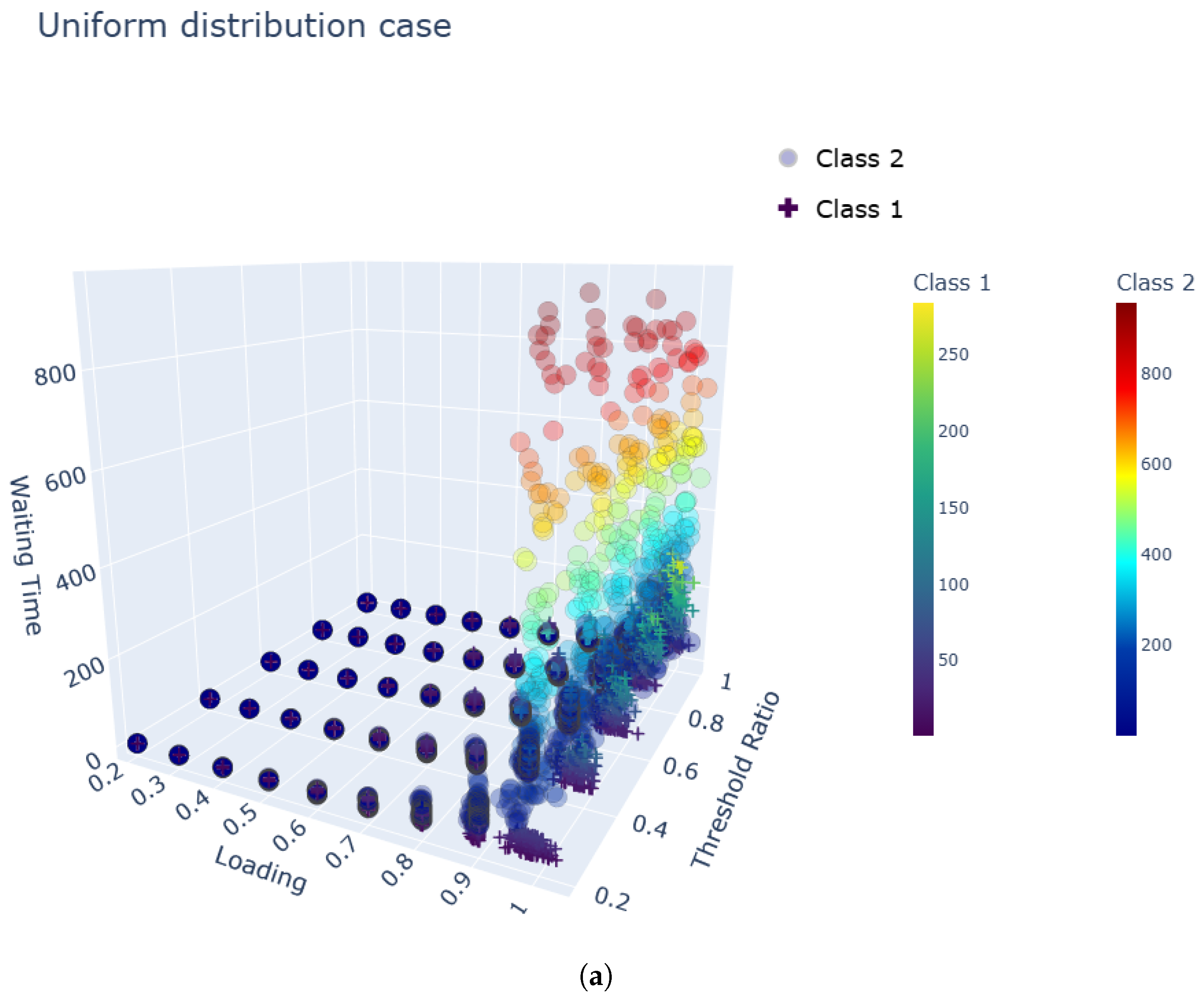
Figure 3a–c demonstrate that the waiting times for both classes increase with higher load and threshold ratios. In particular, the waiting time for Class 2 increases substantially, indicating a heightened sensitivity to system load. Small increases in threshold ratio moderately affect class 1 but severely degrade class 2 performance. Consequently, threshold selection requires careful consideration of class 2 tolerance limits rather than simply optimizing class 1 performance. Furthermore, in the high loading range, class 2 waiting times exhibit near-exponential growth with the threshold ratio, suggesting a critical region beyond which class 2 service becomes severely compromised.
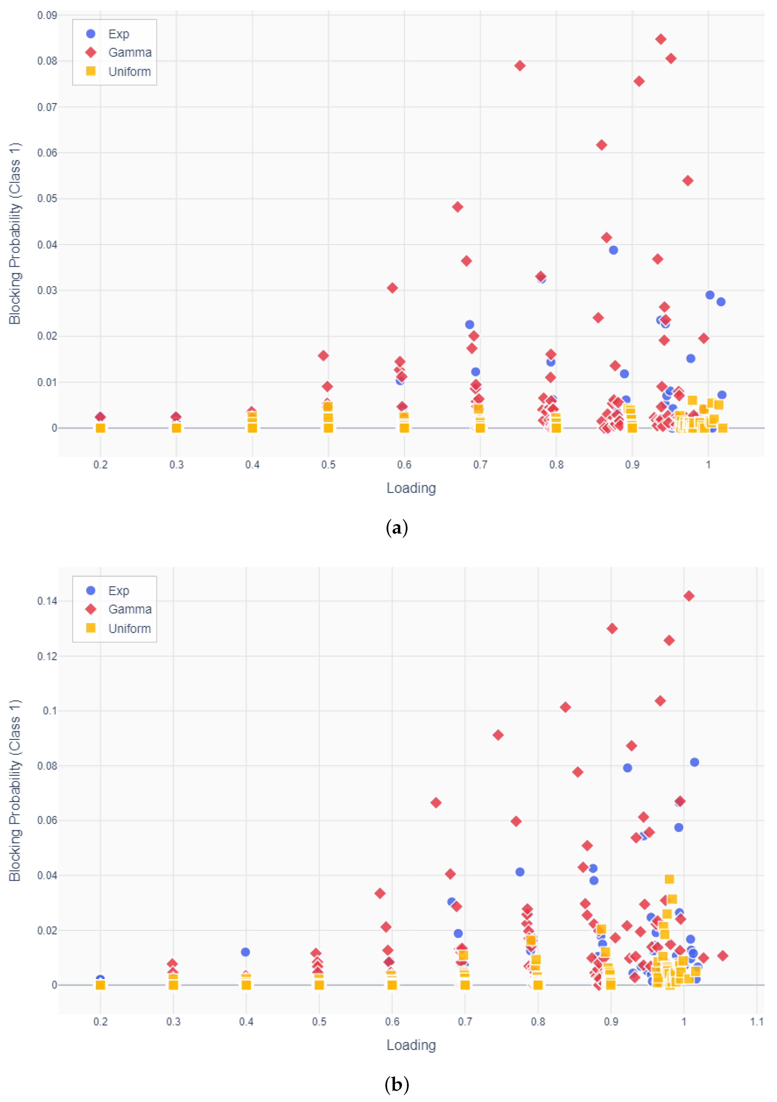
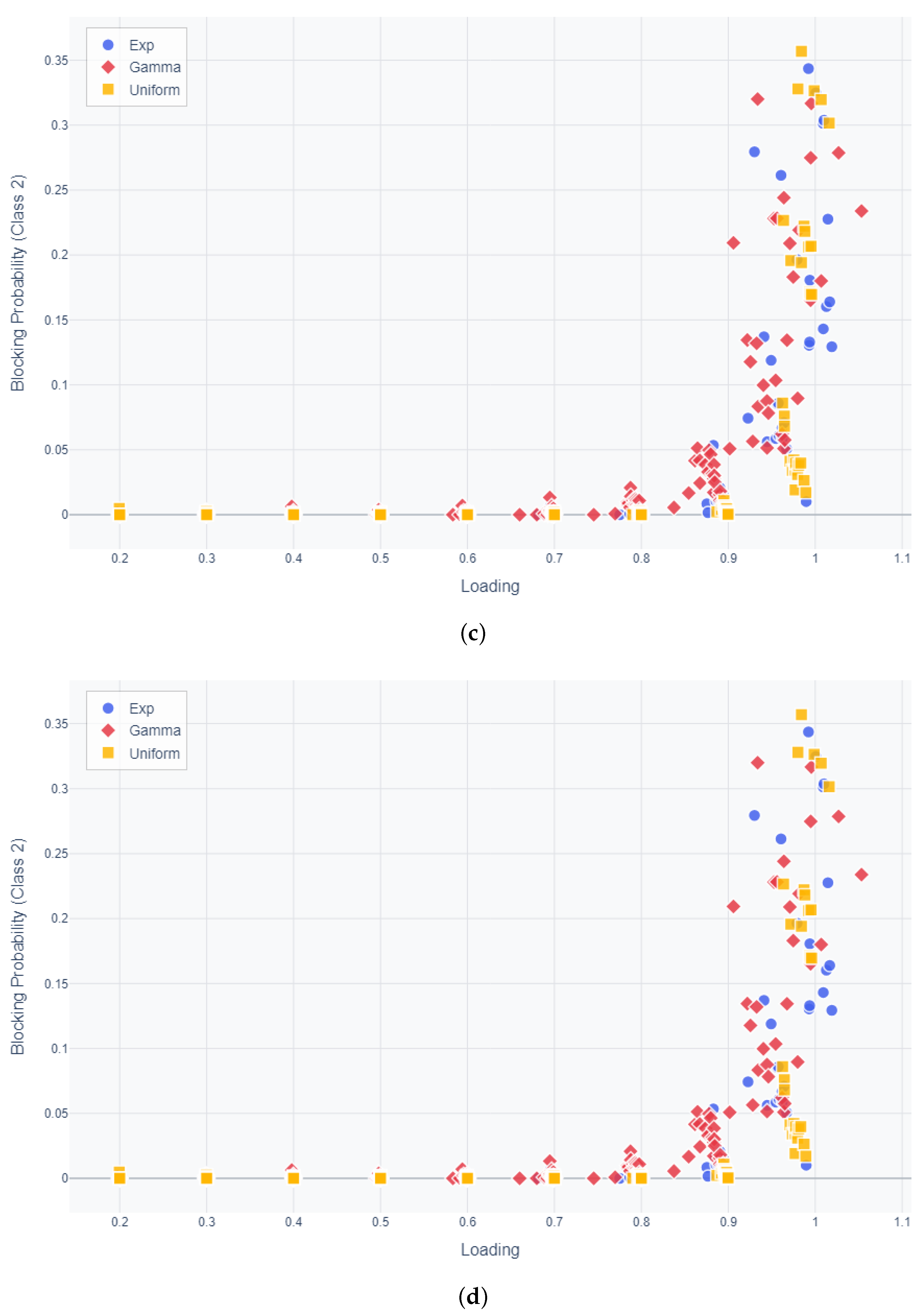
Let us examine the trend in blocking probability. Figure 4a–d show the blocking probability of classes 1 and 2 under three service time distributions and varying loading levels. These figures present two cases where the threshold ratio is 0.2 and 0.8, with the buffer size for class 2 fixed at 20. The threshold ratio represents the proportion used to determine the threshold value relative to the size of buffer 1. Consistently, we observe that higher CV values lead to increased blocking probabilities, which aligns with the trends seen in mean waiting times. As the threshold ratio increases, the blocking probability for class 1 customers increases because a greater number of customers must arrive before the service begins. Conversely, for class 2 customers, the blocking probability decreases as the threshold ratio increases because higher threshold ratios make it more likely that service priority will be allocated to buffer 2.

5. Conclusions

We present a comprehensive analysis of a Markovian queueing model with two finite buffers and an alternating server operating under a queue-length-based threshold-switching policy. By formulating the system as an embedded Markov chain and applying supplementary variable methods, we derived steady-state distributions and key performance metrics, including blocking probabilities and average queue lengths for both customer types. Our results highlight that threshold-based control policies can effectively balance service priorities, preventing excessive delays for high-priority customers, while maintaining acceptable performance for lower-priority traffic. The model’s flexibility allows it to be adapted to various real-world applications, particularly differentiated service provision in telecommunications and dynamic resource allocation in cloud computing and healthcare.
Future research may extend this framework to more general arrival and service processes, including differentiated service time distributions for each customer class, incorporate additional priority classes, or optimize the threshold values for specific performance objectives. Considering the complexity introduced by distinct service time distributions, its rigorous analysis is left as a promising direction for future work. For systems with significantly larger buffer capacities (e.g., K 1 , K 2 > 100 ), developing specialized numerical methods that exploit the block-tridiagonal structure of the transition matrix or employing iterative solution techniques could improve computational efficiency. While our exact analytical approach is well-suited for centralized threshold control with known parameters, we acknowledge that distributed systems with strategic users may benefit from complementary approaches such as game theory or machine learning.

Author Contributions

This paper is the result of the joint work by two authors. D.I.C. designed the methodologies. D.-E.L. conducted the numerical experiment of the mathematical model. D.I.C. and D.-E.L. wrote the original draft. D.I.C. supervised all research processes. D.-E.L. reviewed and edited the final version of the manuscript. All authors have read and agreed to the published version of the manuscript.

Funding

This research was supported by Basic Science Research Program through the National Research Foundation of Korea (NRF) funded by the Ministry of Education (NRF-2017R1D1A3B03028784).

Data Availability Statement

The original contributions presented in this study are included in the article. Further inquiries can be directed to the corresponding author.

Conflicts of Interest

The authors declare no conflicts of interest.

References

  1. Takagi, H. Analysis of Polling Systems; MIT Press: Cambridge, MA, USA, 1986. [Google Scholar]
  2. Boon, M.A.; van der Mei, R.D.; Winands, E.M. Applications of polling systems. Surv. Oper. Res. Manag. Sci. 2011, 16, 67–82. [Google Scholar] [CrossRef]
  3. Borst, S.; Boxma, O. Polling: Past, present, and perspective. Top 2018, 26, 335–369. [Google Scholar] [CrossRef]
  4. Vishnevsky, V.; Semenova, O. Polling systems and their application to telecommunication networks. Mathematics 2021, 9, 117. [Google Scholar] [CrossRef]
  5. Nimisha, M.; Manoharan, M.; Krishnamoorthy, A. Polling Models: A Short Survey and Some New Results. Queueing Model. Serv. Manag. 2024, 7, 25–42. [Google Scholar]
  6. Bruneel, H. Analysis of a threshold-based priority queue. Queueing Syst. 2025, 109, 8. [Google Scholar] [CrossRef]
  7. Lin, W.; Wang, J.Z.; Liang, C.; Qi, D. A threshold-based dynamic resource allocation scheme for cloud computing. Procedia Eng. 2011, 23, 695–703. [Google Scholar] [CrossRef]
  8. Klimenok, V.; Dudin, A.; Dudina, O.; Kochetkova, I. Queuing system with two types of customers and dynamic change of a priority. Mathematics 2020, 8, 824. [Google Scholar] [CrossRef]
  9. Avrachenkov, K.; Perel, E.; Yechiali, U. Finite-buffer polling systems with threshold-based switching policy. Top 2016, 24, 541–571. [Google Scholar] [CrossRef]
  10. Boxma, O.; Perry, D.; Ravid, R.; Yechiali, U. A Polling Model with Threshold Switching. 2024. Preprint. Available online: https://www.eurandom.tue.nl/pre-prints-new/ (accessed on 7 March 2025).
  11. Jolles, A.; Perel, E.; Yechiali, U. Alternating server with non-zero switch-over times and opposite-queue threshold-based switching policy. Perform. Eval. 2018, 126, 22–38. [Google Scholar] [CrossRef]
  12. Borst, S.C.; Boxma, O.J.; Levy, H. The use of service limits for efficient operation of multistation single-medium communication systems. IEEE/ACM Trans. Netw. 1995, 3, 602–612. [Google Scholar] [CrossRef]
  13. Vishnevsky, V.M.; Semenova, O.V.; Bui, D. Investigation of the Stochastic Polling System and Its Applications to Broadband Wireless Networks. Autom. Remote Control 2021, 82, 1607–1613. [Google Scholar] [CrossRef]
  14. Winands, E.; Adan, I.J.B.F.; Van Houtum, G.; Down, D. A state-dependent polling model with k-limited service. Probab. Eng. Informational Sci. 2009, 23, 385–408. [Google Scholar] [CrossRef]
  15. Iliadis, I.; Jordan, L.; Lantz, M.; Sarafijanovic, S. Performance evaluation of tape library systems. Perform. Eval. 2022, 157, 102312. [Google Scholar] [CrossRef]
  16. Boon, M.A.; Adan, I.J.; Winands, E.M.; Down, D.G. Delays at signalized intersections with exhaustive traffic control. Probab. Eng. Informational Sci. 2012, 26, 337–373. [Google Scholar] [CrossRef]
  17. Uncu, N. Load balancing in polling systems under different policies via simulation optimization. Int. J. Simul. Model. 2022, 21. [Google Scholar] [CrossRef]
  18. Wu, Z.; Liu, R.; Pan, E. Server Routing-Scheduling Problem in Distributed Queueing System with Time-Varying Demand and Queue Length Control. Transp. Sci. 2023, 57, 1209–1230. [Google Scholar] [CrossRef]
  19. Dudin, A.; Dudina, O. Analysis of Polling Queueing System with Two Buffers and Varying Service. In Proceedings of the Distributed Computer and Communication Networks: 27th International Conference, DCCN 2024, Moscow, Russia, 23–27 September 2024; Revised Selected Papers. Springer Nature: Berlin/Heidelberg, Germany, 2024; p. 129. [Google Scholar]
  20. Dudin, A.; Sinyugina, Y. Analysis of the Polling System with Two Markovian Arrival Flows, Finite Buffers, Gated Service and Phase-Type Distribution of Service and Switching Times. In Proceedings of the International Conference on Information Technologies and Mathematical Modelling, Tomsk, Russia, 1–5 December 2021; Springer: Berlin/Heidelberg, Germany, 2021; pp. 1–15. [Google Scholar]
  21. Shausan, A.; Vuorinen, A. Thirty-six years of contributions to queueing systems: A content analysis, topic modeling, and graph-based exploration of research published in the QUESTA journal. Queueing Syst. 2023, 104, 3–18. [Google Scholar] [CrossRef]
  22. Dudin, A.; Dudin, S.; Manzo, R.; Rarità, L. Queueing system with batch arrival of heterogeneous orders, flexible limited processor sharing and dynamical change of priorities. AIMS Math. 2024, 9, 12144–12169. [Google Scholar] [CrossRef]
  23. Takács, L. Two queues attended by a single server. Oper. Res. 1968, 16, 639–650. [Google Scholar] [CrossRef]
  24. Eisenberg, M. Two queues with alternating service. SIAM J. Appl. Math. 1979, 36, 287–303. [Google Scholar] [CrossRef]
  25. Boon, M.; Winands, E. Heavy-traffic analysis of k-limited polling systems. Probab. Eng. Informational Sci. 2014, 28, 451–471. [Google Scholar] [CrossRef]
  26. Ozawa, T. Alternating service queues with mixed exhaustive and K-limited services. Perform. Eval. 1990, 11, 165–175. [Google Scholar] [CrossRef]
  27. Perel, E.; Yechiali, U. Two-queue polling systems with switching policy based on the queue that is not being served. Stoch. Model. 2017, 33, 430–450. [Google Scholar] [CrossRef]
  28. Choi, D.I.; Kim, T.S.; Lee, S. Analysis of a queueing system with a general service scheduling function, with applications to telecommunication network traffic control. Eur. J. Oper. Res. 2007, 178, 463–471. [Google Scholar] [CrossRef]
  29. Lee, T.T. M/G/1/N queue with vacation time and exhaustive service discipline. Oper. Res. 1984, 32, 774–784. [Google Scholar] [CrossRef]
Figure 1. Impact of Control Policy on Waiting Time Distribution of Class 1.
Mathematics 13 03555 g001
Figure 2. Distribution of Waiting Times by Service Time Distribution and System Load. (a) Waiting time of class 1 over different loading levels. (b) Waiting time of class 2 over different loading levels.
Mathematics 13 03555 g002
Figure 3. Class-wise mean waiting times by service time distribution and system loading level. (a) Mean waiting time under uniform service distribution. (b) Mean waiting time under exponential service distribution. (c) Mean waiting time under gamma service distribution.
Mathematics 13 03555 g003aMathematics 13 03555 g003b
Figure 4. Blocking probability across service time distributions and threshold ratios, with buffer 2 size fixed at 20. (a) Blocking probability for Class 1 (threshold ratio = 0.2). (b) Blocking probability for Class 1 (threshold ratio = 0.8). (c) Blocking probability for Class 2 (threshold ratio = 0.2). (d) Blocking probability for Class 2 (threshold ratio = 0.8).
Mathematics 13 03555 g004aMathematics 13 03555 g004b
Table 1. Settings for Service Time Distributions and System Parameters.
CategoryDescription
Service Time DistributionsAll service time distributions have a mean of 10 but differ in CV: Uniform(5, 15) with CV = 0.3; Exponential distribution with rate = 0.1 (CV = 1.0); Gamma distribution with a shape parameter of 0.44 and a scale parameter of 22.52 (CV = 1.4).
Arrival Rate per ClassArrival rates for each class range from 0.01 to 0.06.
Class 1 Buffer SizeBuffer sizes range from 5 to 25 in increments of 5. The threshold is set as a proportion of the buffer size, with ratios ranging from 0.2 to 1.0. For example, if the buffer size is 5 and the ratio is 0.2, the threshold is 1.
Class 2 Buffer SizeBuffer sizes range from 10 to 40 in increments of 10.
Disclaimer/Publisher’s Note: The statements, opinions and data contained in all publications are solely those of the individual author(s) and contributor(s) and not of MDPI and/or the editor(s). MDPI and/or the editor(s) disclaim responsibility for any injury to people or property resulting from any ideas, methods, instructions or products referred to in the content.