Rapid Deterioration of Convergence in Taylor Expansions of Linearizing Maps of Hénon Maps at Hyperbolic Fixed Points

Abstract

In this paper, we prove that the Taylor expansions of analytic functions appearing in the linearization of quadratic maps at hyperbolic fixed points do not successfully approximate invariant manifolds, such as stable and unstable manifolds, when higher-order terms are truncated. This fact was pointed out by Newhouse et al. in their numerical experiments, and implies that the Taylor expansions are inadequate for quantitatively studying dynamical systems such as quadratic maps. In fact, it is shown that the computational complexity for the approximations by the Taylor expansions grows exponentially.

1. Introduction

The Hénon map $f:{\mathbb{C}}^2\to {\mathbb{C}}^2$ is a quadratic map defined by

$$\begin{array}{c}\hfill f:\left(x,y\right)\mapsto \left(1+y-a{x}^2,bx\right),\end{array}$$

where $a,b\in \mathbb{C}$ are parameters, and $a\ne 0,b\ne 0$ ([1]). Let $P=(x_f,y_f)$ be one of the fixed points of f, and let ${\alpha }_1,{\alpha }_2$ be the eigenvalues of the derivative $D_{P}f$. Throughout this paper, we assume

$$|{\alpha }_1|\ne 1$$

and set $\alpha ={\alpha }_1$. Then

$${\alpha }^2-\lambda \alpha -b=0$$

holds, where $\lambda =-2a{x}_f$. Two cases occur: $0<\left|\alpha \right|<1$ and $\left|\alpha \right|>1$. We recall that P is hyperbolic when $|{\alpha }_2|\ne 1$ in addition. If $\left|\alpha \right|<1<|{\alpha }_2|$ or $|{\alpha }_2|<1<|\alpha |$, then P is a saddle. This paper treats the case satisfying the following condition:

$$\alpha \ne {\alpha }_2,$$

which is more general than the saddle case.

The following result on the linearization of dynamical systems is well-known (cf. [2]).

Proposition 1. 

(Poincaré [3]) Under the above assumptions, for any eigenvector $v\ne 0$ for α, there uniquely exists a holomorphic map ${\mathcal{P}}_{\alpha }:\mathbb{C}\to {\mathbb{C}}^2$ satisfying ${\mathcal{P}}_{\alpha }\left(0\right)=P$ and ${\mathcal{P}}_{\alpha }^{\prime }\left(0\right)=v$ such that

$$\begin{array}{c}\hfill f\circ {\mathcal{P}}_{\alpha }\left(t\right)={\mathcal{P}}_{\alpha }\left(\alpha t\right)\end{array}$$

(1)

for all $t\in \mathbb{C}$. Furthermore, ${\mathcal{P}}_{\alpha }:\mathbb{C}\to {\mathbb{C}}^2$ is injective and for all $t\in \mathbb{C}$, ${\mathcal{P}}_{\alpha }^{\prime }\left(t\right)\ne 0$.

The map ${\mathcal{P}}_{\alpha }:\mathbb{C}\to {\mathbb{C}}^2$ in Proposition 1 is called Poincaré’s map. The image

$$W_{\alpha }\left(P\right)={\mathcal{P}}_{\alpha }\left(\mathbb{C}\right)$$

is the invariant manifold associated with $\alpha$, which coincides with the stable or unstable manifold when P is a saddle. By Proposition 1, $W_{\alpha }\left(P\right)$ is actually f-invariant (i.e., $f\left(W_{\alpha }\left(P\right)\right)=W_{\alpha }\left(P\right)$) and an injective immersed submanifold of ${\mathbb{C}}^2$ through P. We equip the intrinsic metric on $W_{\alpha }\left(P\right)$ induced by ${\mathcal{P}}_{\alpha }$.

Franceschini and Russo [4] used Poincaré’s map for numerical calculations to detect homoclinic points in the case where a and b are the original Hénon’s parameter values. Also, Fornaess and Gavosto [5,6] investigated the existence of homoclinic tangencies using Poincaré’s map. The existence of higher-dimensional Poincaré’s maps was investigated by Cabré, Fontich, and de la Llave [7,8,9]. Anastassiou, Bountis, and Bäcker [10] used their result to detect homoclinic points for the 4-dimensional maps. Also, Newhouse, Berz, Grote and Makino [11] estimated the topological entropy of the Hénon map using symbolic dynamics via the Taylor models in addition to Poincaré’s map. We emphasize that Poincaré’s maps were expressed in Taylor expansions in those studies.

It is important to clarify how the Taylor expansions work for quantitative studies of dynamical systems, such as numerically calculating the topological entropy or detecting the homoclinic set (cf. [11,12,13]). In this paper, we prove that the computational complexity for the approximations by the Taylor expansions grows exponentially, which is precisely stated as follows.

Theorem 1.

When $0<\left|\alpha \right|<1$ (resp. $\left|\alpha \right|>1$), if the disk centered at P with radius ${\left|\alpha \right|}^{-L}$ (resp. ${\left|\alpha \right|}^L$) in the invariant manifold $W_{\alpha }\left(P\right)$ with respect to the intrinsic metric is computationally realized with high computational accuracy in ${\mathbb{C}}^2$ by the map ${\mathcal{P}}_{\alpha }$, then the order of the truncation terms in the Taylor expansions of ${\mathcal{P}}_{\alpha }$ must be greater than N satisfying the condition

$$\begin{array}{c}\hfill N\sim 2^L,\end{array}$$

(2)

where L is a natural number given arbitrarily.

This result implies that the Taylor expansions are inadequate for quantitative studies such as numerically calculating the topological entropy or detecting the homoclinic set, which was pointed out by Newhouse, Berz, Grote, and Makino [11] in their numerical experiments.

2. Main Results

To state the main results of the current paper, we mention the construction of Poincaré’s map ${\mathcal{P}}_{\alpha }$. For simplicity, let us consider a conjugate map $f:{\mathbb{C}}^2\to {\mathbb{C}}^2$ of the above map by the translation $(x+x_0,y+y_0)\mapsto (x,y)$ on ${\mathbb{C}}^2$ sending P to the origin $O=(0,0)$, i.e.,

$$\begin{array}{c}\hfill f:\left(x,y\right)\mapsto \left(\lambda x+y-a{x}^2,bx\right).\end{array}$$

Set

$$\begin{array}{c}\hfill {\mathcal{P}}_{\alpha }\left(s\right)=\left(x_p\left(s\right),y_p\left(s\right)\right)(s\in \mathbb{C}).\end{array}$$

Then, from the relation (1), we have

$$\begin{array}{c}\hfill x_p\left(\alpha t\right)-\lambda x_p\left(s\right)-b{x}_p\left({\alpha }^{-1}s\right)=-a{\left\{x_p\left(s\right)\right\}}^2\end{array}$$

(3)

and $y_p\left(s\right)=b{x}_p\left({\alpha }^{-1}s\right)$. Setting a series expansion

$$\begin{array}{c}\hfill x_p\left(s\right)=\sum _{n=1}^{\infty }{a}_n{s}^n,\end{array}$$

(4)

and substituting this into the above relation (3), we obtain by the coefficient comparison

$$\begin{array}{c}\hfill a_n=-{\displaystyle \frac{a}{D_n}}\sum _{k=1}^{n-1}{a}_k{a}_{n-k}(\forall n\ge 2),\end{array}$$

(5)

where $D_n={\alpha }^n-\lambda -b{\alpha }^{-n}$. Note that the non-resonance condition that $D_n\ne 0$ for all $n\ge 2$ is assumed here. This condition is automatically satisfied when P is a saddle. The first-order coefficient $a_1$ is determined by the condition ${\mathcal{P}}^{\prime }\left(0\right)=v$, and $a_1\ne 0$.

Choosing ${\zeta }_1$ as a branch of $-log\alpha$, we introduce a new variable $t\in \mathbb{C}$ by the transformation

$$\begin{array}{c}\hfill s={\mathrm{e}}^{-{\zeta }_{1}t},\end{array}$$

and define $x\left(t\right)=x_p\left(s\right)$. Let $y\left(t\right)=bx(t-1)$. We define a holomorphic map $\mathcal{S}:\mathbb{C}\to {\mathbb{C}}^2$ by $\mathcal{S}\left(t\right)=\left(x\right(t),y(t\left)\right)$. Then, from the relation (1), it follows that by the l-th iteration ($l\in \mathbb{Z}$) of f, any point in the invariant manifold $W_{\alpha }\left(P\right)$ is mapped as follows:

$$\begin{array}{c}\hfill f^l\circ S\left(t\right)=S(t+l).\end{array}$$

(6)

For each $n\ge 1$, let

$$\begin{array}{c}\hfill x_n\left(t\right)=a_n{\mathrm{e}}^{-{\zeta }_{1}nt}.\end{array}$$

Then from (4), we have

$$\begin{array}{c}\hfill x\left(t\right)=x_p\left(s\right)=\sum _{n=1}^{\infty }{x}_n\left(t\right).\end{array}$$

(7)

We discuss the convergence of the series (7), assuming that $t\in \mathbb{C}$ are given arbitrarily.

2.1. Rapid Deterioration of Convergence in Taylor Expansions

Write $-{\zeta }_1={\zeta }_{1r}+i{\zeta }_{1i}$ and $t=t_r+i{t}_i$ in the form of real and imaginary parts. For simplicity, we set

$$E_1={\displaystyle \frac{log\left(\right|2a{a}_1\left|{\mathrm{e}}^{-{\zeta }_{1i}{t}_i}\right)}{log\left|\alpha \right|}},$$

and let

$$\begin{array}{c}\hfill r_{\alpha ,t}=\left\{\begin{array}{cc}{\mathrm{e}}^{-E_{1}log2-1-t_r log2}\hfill & \mathrm{if}0<\left|\alpha \right|<1,\hfill \\ {\mathrm{e}}^{E_{1}log2-1+t_r log2}\hfill & \mathrm{if}\left|\alpha \right|>1.\hfill \end{array}\right.\end{array}$$

(8)

Define a natural number $n_t$ as

$$n_t=\left[r_{\alpha ,t}\right],$$

where $[·]$ denotes the Gauss’s symbol. We notice that $n_t$ grows exponentially with respect to $t_r$, if $t_r$ is chosen to be negative when $0<\left|\alpha \right|<1$, and to be positive when $\left|\alpha \right|>1$, respectively.

The purpose of this paper is to give a lower bound to the magnitude of each higher-order term of the series (7) as follows.

Theorem 2.

There exists a constant $N_1$ such that if $n_t>N_1$ and $N_1<n_t+k<2n_t$ ($k\in \mathbb{Z}$) are satisfied, and if $\delta =k/n_t$ is close to zero, then there is ϵ with $0\le ϵ\ll n_t$ such that

$$\begin{array}{c}\hfill |x_{n_t+k}\left(t\right)|\ge \left\{\begin{array}{cc}{\left|\alpha \right|}^{-{\displaystyle \frac{n_t}{log2}}(1-{\displaystyle \frac{{\delta }^2}{2}})+ϵ}\hfill & \mathrm{if}0<\left|\alpha \right|<1,\hfill \\ {\left|\alpha \right|}^{{\displaystyle \frac{n_t}{log2}}(1-{\displaystyle \frac{{\delta }^2}{2}})-ϵ}\hfill & \mathrm{if}\left|\alpha \right|>1.\hfill \end{array}\right.\end{array}$$

(9)

The above result gives a mathematical description of the fact that the approximation of $x_p\left(s\right)$ described by the Taylor expansion (4) or (7) rapidly deteriorates as the value $\left|s\right|$ becomes large when higher-order terms are truncated.

To state how the series (4) converges, let us denote by $E_N\left(s\right)$ the remainder term:

$$\begin{array}{c}\hfill E_N\left(s\right)=\sum _{n=N}^{\infty }{a}_n{s}^n=\sum _{n=N}^{\infty }{x}_n\left(t\right),s=e^{-{\zeta }_{1}t},\end{array}$$

(10)

where N is a natural number. The following estimate holds.

Theorem 3.

Let $0<\left|\alpha \right|<1$. Then there exists a constant $K>1$ such that for every $R>0$, if a natural number N with $N>N_1$ is large enough, the remainder term $E_N\left(s\right)$ is estimated as

$$\begin{array}{c}\hfill {\displaystyle \frac{1}{2}}|2a{a}_1{|}^N{\left|s\right|}^N{\left|\alpha \right|}^{{\displaystyle \frac{NlogN}{log2}}}\le |E_N\left(s\right)|\le 2K^N{\left|s\right|}^N{\left|\alpha \right|}^{{\displaystyle \frac{N(logN-\text{log} \text{log} N)}{log2}}}\end{array}$$

(11)

for any s with $\left|s\right|\le R$, where $N_1$ is the constant stated in Theorem 2. When $\left|\alpha \right|>1$, a similar statement holds if α is replaced with ${\alpha }^{-1}$.

Theorem 1 is obtained from Theorem 3 as follows.

Proof of Theorem 1. 

Let $\left|s\right|\sim 1$ for $0<\left|\alpha \right|<1$. If the higher-order terms in the series (4) are truncated after N-th, the error E for the point $\mathcal{P}\left({\alpha }^{-L}s\right)$ is estimated as

$$E\sim {\left({\left|\alpha \right|}^{{\displaystyle \frac{logN}{log2}}}\left|{\alpha }^{-L}\right|\right)}^N$$

by (11). If the right-hand side of this estimate is small enough, we need the condition that

$${\displaystyle \frac{logN}{log2}}-L>0,$$

which is equivalent to $N>2^L$. Thus, we obtain the necessary condition (2). In the same way as above, we obtain the conclusion for the case of $\left|\alpha \right|>1$. The proof of Theorem 1 is complete. □

2.2. Discussion: Beyond Taylor Series

The following examples 1 and 2 specifically illustrate how pessimistic the implications of Theorems 2 and 3 are.

Example 1.

Let $0\le t_0\le 1$ be an initial time, and let $0<\left|\alpha \right|<1$. When $l=-10$ and $t=t_0+l$, we have from (8) that $n_t=\left[r_{\alpha .t}\right]\sim 400$ (we set $E_1=0$ and $t_i=0)$. Then (9) gives

$$|x_{n_t}(t_0-10){|\ge |\alpha |}^{{\displaystyle \frac{-400}{log2}}}\sim {\left|\alpha \right|}^{-570}.$$

In this case, the computation is yet computationally feasible. On the other hand, when $l=-20$ and $t=t_0+l$, (8) gives $n_t\sim 4.4\times {10}^5$ and by (9) we have

$$|x_{n_t}(t_0-20){| \ge |\alpha |}^{{\displaystyle \frac{-4.4\times {10}^5}{log2}}}\sim {\left|\alpha \right|}^{-6 \times {10}^5},$$

which implies that the computation is infeasible.

Example 2.

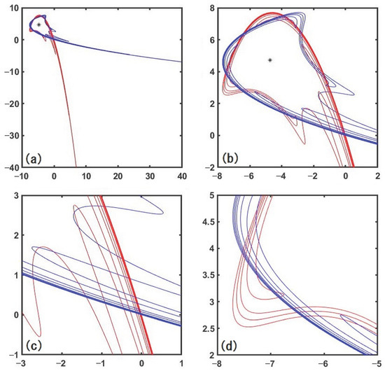
Here, we present an example of stable and unstable manifolds depicted by using the Taylor expansion (7). Figure 1 shows a chaotic system encircling KAM tori in a symplectic case. We select the eigenvalues α as $\alpha ={\alpha }_1={\mathrm{e}}^{-1.2}$ for the stable manifold and $\alpha ={\alpha }_2={\mathrm{e}}^{1.2}$ for the unstable manifold, respectively. Then, the dynamical parameter $b=-{\alpha }_1{\alpha }_2$ satisfies $b=-1$. Also λ and a in (3) are given as $\lambda =2cosh\left(1.2\right)$ and $a=-1+{\left(\lambda /2-1\right)}^2\sim -0.34284$, respectively. For these parameters, one fixed point is elliptic ($\left|\alpha \right|=1$) and the other is a saddle point. The eigenvalues ${\alpha }_1$ and ${\alpha }_2$ at the saddle point [$(x,y)=(0,0)$ here] are ${\alpha }_1=0.30119$ (stable) and ${\alpha }_2=3.32012$ (unstable). For $\alpha ={\alpha }_1$, the branch ${\zeta }_1$ is chosen as ${\zeta }_1=1.2$ and the variable t is selected to be real numbers with ranges $t\ge -9.65$ and $t\ge -1.65$ by setting $a_1=-{\displaystyle \frac{sinh(-1.2)}{2a}}$ and $a_1={\displaystyle \frac{sinh(-1.2)}{2a}}$, respectively. When $t=-9.65$, (8) gives $n_t\sim 375$. We similarly choose the branch ${\zeta }_1$ and the variable t for $\alpha ={\alpha }_2$. In this numerical computation, we take the number of truncation N in the series (7) as $N=4000$. Concentric KAM tori (and periodic orbits) exist inside the chaotic system. The number $N_1$ in Theorem 2 in this example is $N_1\sim 560$ for $\alpha ={\alpha }_1$.

Figure 1. A chaotic system encircling KAM tori, where $a=-0.34284$ and $b=-1$. The asterisk denotes an elliptic fixed point. Panel (b) is the enlarged figure of (a), and panels (c,d) are further enlarged views of (b). The red and blue curves denote the stable and unstable manifolds, respectively.

To improve the pessimistic situation as stated above, Newhouse, Berz, Grote, and Makino [11] introduced the notion of the Taylor models by restricting the parameter s such that the set ${\left\{{\mathcal{P}}_{\alpha }\left({\alpha }^{\ell }s\right)\right\}}_{\ell =0}^{\infty }$ ($0<\left|\alpha \right|<1)$ or ${\left\{{\mathcal{P}}_{\alpha }\left({\alpha }^{-\ell }s\right)\right\}}_{\ell =0}^{\infty }$ ($\left|\alpha \right|>1)$ is contained in a given bounded set, in which they rigorously estimated the topological entropy of Hénon maps using symbolic dynamics. See also Ishii [12].

In correspondence to such a development, it has been obtained very recently by the authors that the holomorphic maps $f^{-\ell }\circ {\mathcal{P}}_{\alpha ,N}\left({\alpha }^{\ell }s\right)$ defined by taking conjugates by iteration maps of the Hénon map and of the derivative give much better approximations of ${\mathcal{P}}_{\alpha }$ theoretically and numerically when the parameter s is restricted as above, where ${\mathcal{P}}_{\alpha ,N}:\mathbb{C}\to {\mathbb{C}}^2$ is the polynomial map with degree N when higher-order terms are truncated from ${\mathcal{P}}_{\alpha }$.

It is well-known that the method of contraction mappings is useful in studying invariant manifolds and dynamical stability (cf. [14]). Such a method might also work for the approximation of ${\mathcal{P}}_{\alpha }$ theoretically and numerically.

The invariant manifold $W_{\alpha }\left(P\right)$ can be described by a divergent series called asymptotic expansion in Poincaré’s sense, and a phenomenon similar to the Stokes phenomenon and to differential equation theory occurs. For details, we can refer to Tovbis [15], Lazutkin, Schachmannski and Tabanov [16], Gelfreich and Sauzin [17], Lazutkin, Segur and Hakim [16,18,19], Écalle [20,21,22], Sternin and Shatalov [23], Voros [24], and Matsuoka and Hiraide [13,25,26,27]. The results of those studies have made it possible to quantitatively investigate the dynamical system of the Hénon map f with extremely high precision using computers, which suggests that the asymptotic expansion gives us much better performance than the ones stated in Theorems 2 and 3. The authors hope that the research area will be developed in discrete dynamical systems.

3. Proofs of Theorems 2 and 3

To prove Theorems 2 and 3, we prepare the following Lemmas 1 and 2, which gives sharp estimates on upper and lower bounds to absolute values of the coefficients $a_n$ ($n\ge 1$) (cf. [5,6]). In the following, suppose that $0<\left|\alpha \right|<1$.

Lemma 1.

There exists a constant $K>1$ such that

$$\begin{array}{c}\hfill |a_n|<K^n{\left|\alpha \right|}^{{\displaystyle \frac{n(logn-\text{log}{\text{log}}_{+}n)}{log2}}}\end{array}$$

(12)

holds for all $n\ge 1$, where ${log}_{+}n=\max \{logn,1\}$.

Lemma 2.

There exists a natural number $N_1\ge 1$ such that

$$\begin{array}{c}\hfill |a_n| \ge |2a{a}_1{|}^n{\left|\alpha \right|}^{{\displaystyle \frac{nlogn}{log2}}}\end{array}$$

(13)

holds for all $n\ge N_1$.

The above results are stronger than the estimate obtained by Fornaess and Gavosto [5,6] via complex analysis.

Lemmas 1 and 2 also hold for $\left|\alpha \right|>1$, if $\alpha$ is replaced with ${\alpha }^{-1}$. The proofs of Lemmas 1 and 2 are provided in Section 4 and Section 5, respectively.

Define a real function

$$\begin{array}{c}\hfill F(r,t)=E_{1}r+{\displaystyle \frac{rlogr}{log2}}+t_{r}r(r\ge 1).\end{array}$$

Then, we have

$${\displaystyle \frac{\partial F}{\partial r}}(r_{\alpha ,t},t)=0,$$

which is equivalent to the relation (8) because the case of $0<\left|\alpha \right|<1$ is considered. It follows that $F(r,t)$ takes its minimum value at $r=r_{\alpha ,t}$ for a fixed t.

Let

$$E_2={\displaystyle \frac{log\left(K{\mathrm{e}}^{-{\zeta }_{1i}{t}_i}\right)}{log\left|\alpha \right|}},$$

where $K>1$ is the constant stated in Lemma 1, and define a real function

$$G(r,t)=E_{2}r+{\displaystyle \frac{r(logr-\text{log}{\text{log}}_{+}r)}{log2}}+t_{r}r(r\ge 1).$$

By using Lemmas 1 and 2, the following Lemma 3 is easily checked.

Lemma 3.

If $N_1\ge 1$ is the number as in Lemma 2,

$$\begin{array}{c}\hfill {\left|\alpha \right|}^{F(n,t)}\le |x_n{\left(t\right)|\le |\alpha |}^{G(n,t)}\end{array}$$

(14)

holds for any $n\ge N_1$.

Proof of Theorem 2. 

Let ${ϵ}^{\prime }=log{r}_{\alpha ,t}-log{n}_t$. Obviously, $0\le {ϵ}^{\prime }\ll 1$. From (8), we have

$$log{n}_t=-E_{1}log2-1-t_{r}log2-{ϵ}^{\prime },$$

which implies that

$${\displaystyle \frac{n_{t}log{n}_t}{log2}}=-E_1{n}_t-{\displaystyle \frac{n_t}{log2}}-t_r{n}_t-{\displaystyle \frac{{ϵ}^{\prime }{n}_t}{log2}}.$$

Let $N_1\ge 1$ be the number as in Lemma 2. Since

$$\begin{array}{c}\hfill {\displaystyle \frac{(n_t+k)log(n_t+k)}{log2}}={\displaystyle \frac{n_{t}log{n}_t}{log2}}+{\displaystyle \frac{n_{t}log\left(1+\frac{k}{n_t}\right)}{log2}}+{\displaystyle \frac{klog{n}_t}{log2}}+{\displaystyle \frac{klog\left(1+\frac{k}{n_t}\right)}{log2}},\end{array}$$

by Lemma 3 we obtain

$$\begin{array}{ccc}\hfill \left|x_{n_t+k}\left(t\right)\right|& \ge & {\left|\alpha \right|}^{F(n_t+k,t)}\hfill \\ & =& {\left|\alpha \right|}^{E_{1}k-{\displaystyle \frac{n_t}{log2}}+{\displaystyle \frac{n_{t}log\left(1+\frac{k}{n_t}\right)}{log2}}+{\displaystyle \frac{klog{n}_t}{log2}}+{\displaystyle \frac{klog\left(1+\frac{k}{n_t}\right)}{log2}}-t_{r}k-{\displaystyle \frac{{ϵ}^{\prime }{n}_t}{log2}}}\hfill \\ & =& {\left|\alpha \right|}^{{\displaystyle \frac{n_{t}log\left(1+\frac{k}{n_t}\right)}{log2}}-{\displaystyle \frac{(n_t+k)}{log2}}+{\displaystyle \frac{klog\left(1+\frac{k}{n_t}\right)}{log2}}-{\displaystyle \frac{{ϵ}^{\prime }(n_t+k)}{log2}}}.\hfill \end{array}$$

(15)

Taking $\left|k\right|\ll n_t$ into account, we have

$$\begin{array}{ccc}\hfill n_{t}log\left(1+{\displaystyle \frac{k}{n_t}}\right)-k& =& n_t\left({\displaystyle \frac{k}{n_t}}-{\displaystyle \frac{1}{2}}{\left({\displaystyle \frac{k}{n_t}}\right)}^2+\cdots \right)-k=n_t\left(-{\displaystyle \frac{1}{2}}{\left({\displaystyle \frac{k}{n_t}}\right)}^2+O\left[{\left({\displaystyle \frac{k}{n_t}}\right)}^3\right]\right),\hfill \\ \hfill klog\left(1+{\displaystyle \frac{k}{n_t}}\right)& =& k\left({\displaystyle \frac{k}{n_t}}-{\displaystyle \frac{1}{2}}{\left({\displaystyle \frac{k}{n_t}}\right)}^2+\cdots \right)=n_t\left({\left({\displaystyle \frac{k}{n_t}}\right)}^2+O\left[{\left({\displaystyle \frac{k}{n_t}}\right)}^3\right]\right).\hfill \end{array}$$

Then (15) yields the inequality (9). In the same way as above, we obtain the conclusion for the case of $\left|\alpha \right|>1$. The proof of Theorem 2 is complete. □

Proof of Theorem 3. 

Let us express $\left|E_p\left(s\right)\right|$ as

$$\begin{array}{ccc}\hfill \left|E_p\left(s\right)\right|& =& \left|a_N{s}^N\right||1+h\left(s\right)|,\hfill \end{array}$$

where

$$\begin{array}{ccc}\hfill h\left(s\right)& =& {\displaystyle \frac{a_{N+1}}{a_N}}s+{\displaystyle \frac{a_{N+2}}{a_N}}{s}^2+\cdots \hfill \\ & =& {\displaystyle \frac{x_{N+1}\left(t\right)}{x_N\left(t\right)}}+{\displaystyle \frac{x_{N+2}\left(t\right)}{x_N\left(t\right)}}+\cdots .\hfill \end{array}$$

Let $N\ge N_1$. Then, from Lemma 3 we can estimate $\left|h\right(s\left)\right|$ as

$$\begin{array}{c}\hfill \left|h\left(s\right)\right|\le \sum _{m=1}^{\infty }{\left|\alpha \right|}^{G(N+m,t)-F(N,t)}.\end{array}$$

(16)

Let $R>0$ be given arbitrarily. Choosing $N>N_1$ to be sufficiently large, we have that if

$$\left|s\right|=e^{-{\zeta }_{1i}{t}_i+{\zeta }_{1r}{t}_r}\le R$$

is satisfied, then

$$G(N+m,t)-F(N,t)\ge (N+m)log(N+m)-NlogN$$

holds for any $m\ge 1$. Then, from (16) it follows that

$$\begin{array}{c}\hfill \left|h\left(s\right)\right|\le \sum _{m=1}^{\infty }{\left({\displaystyle \frac{1}{{(N+1)}^{log|{\alpha }^{-1}|}}}\right)}^m.\end{array}$$

Since

$$\begin{array}{c}\hfill \left|a_N{s}^N\right|(1-|h\left(s\right)\left|\right)\le |E_p\left(s\right)|\le \left|a_N{s}^N\right|(1+|h\left(s\right)\left|\right),\end{array}$$

(17)

the conclusion is obtained from Lemmas 1 and 2. In the same way as above, we obtain the conclusion for the case of $\left|\alpha \right|>1$. The proof of Theorem 3 is complete. □

4. Proof of Lemma 1

In this section, we give the proof of Lemma 1

Since $0<\left|\alpha \right|<1$, by the definition, there exists a constant $C>1$ such that

$$\begin{array}{c}\hfill \left|{\displaystyle \frac{a}{D_n}}\right|{\left|\alpha \right|}^{-n}<C\end{array}$$

(18)

holds for all $n\ge 1$, and then we can choose $n_0\ge 5$ such that

$$\begin{array}{c}\hfill {C\left|\alpha \right|}^{{\displaystyle \frac{n+1+\frac{logn}{log\left|\alpha \right|}log(n+1)}{log(n+1)}}}\le 1\end{array}$$

(19)

is satisfied for any $n\ge n_0$. Take a constant $K>1$ such that the inequality (12) holds for $1\le n\le n_0$. Let $n\ge n_0$, and assume that $a_1,a_2,\cdots ,a_{n-1}$ and $a_n$ satisfy the inequality (12).

Then we have

$$\begin{array}{ccc}& & |a_{n+1}|=\left|{\displaystyle \frac{a}{D_{n+1}}}\right||a_1{a}_n+a_2{a}_{n-1}+\cdots a_n{a}_1|\le \left|{\displaystyle \frac{a}{D_{n+1}}}\right|\sum _{k=1}^n\left|a_k{a}_{n+1-k}\right|\hfill \\ & \le & \left|{\displaystyle \frac{a}{D_{n+1}}}\right|\sum _{k=1}^n{K}^{n+1}{\left|\alpha \right|}^{{\displaystyle \frac{k}{log2}}(logk-log{log}_{+}k)+{\displaystyle \frac{n+1-k}{log2}}\left[log(n+1-k)-log{log}_{+}(n+1-k)\right]}.\hfill \end{array}$$

Noticing $n\ge n_0\ge 5$, we have the result that the exponent part of $\left|\alpha \right|$ in the above inequality takes the minimum value at $k=(n+1)/2$. Therefore,

$$\begin{array}{ccc}& & |a_{n+1}|\le n\left|{\displaystyle \frac{a}{D_{n+1}}}\right|K^{n+1}{\left|\alpha \right|}^{{\displaystyle \frac{n+1}{log2}}log{\displaystyle \frac{n+1}{2}}-{\displaystyle \frac{n+1}{log2}}log{log}_{+}{\displaystyle \frac{n+1}{2}}}\hfill \\ & =& n\left|{\displaystyle \frac{a}{D_{n+1}}}\right|K^{n+1}{\left|\alpha \right|}^{-(n+1)+{\displaystyle \frac{n+1}{log2}}log(n+1)-{\displaystyle \frac{n+1}{log2}}log{log}_{+}(n+1)-{\displaystyle \frac{n+1}{log2}}log\left(1-{\displaystyle \frac{log2}{log(n+1)}}\right)}.\hfill \end{array}$$

Using the expansion

$$log\left(1-{\displaystyle \frac{log2}{log(n+1)}}\right)=-{\displaystyle \frac{log2}{log(n+1)}}-{\displaystyle \frac{1}{2}}{\left({\displaystyle \frac{log2}{log(n+1)}}\right)}^2-\cdots ,$$

we obtain by (18) and (19) that

$$\begin{array}{ccc}\hfill |a_{n+1}|& \le & n\left|{\displaystyle \frac{a}{D_{n+1}}}\right|K^{n+1}{\left|\alpha \right|}^{-(n+1)+{\displaystyle \frac{n+1}{log(n+1)}}+{\displaystyle \frac{n+1}{log2}}\left[log(n+1)-log{log}_{+}(n+1)\right]}\hfill \\ & \le & C{K}^{n+1}{\left|\alpha \right|}^{{\displaystyle \frac{n+1+\frac{logn}{log\left|\alpha \right|}log(n+1)}{log(n+1)}}}{\left|\alpha \right|}^{{\displaystyle \frac{n+1}{log2}}\left[log(n+1)-log{log}_{+}(n+1)\right]}\hfill \\ & \le & K^{n+1}{\left|\alpha \right|}^{{\displaystyle \frac{n+1}{log2}}\left[log(n+1)-log{log}_{+}(n+1)\right]},\hfill \end{array}$$

which implies that the inequality (12) holds for $n+1$. Therefore, the conclusion is obtained. The proof of Lemma 1 is complete.

In the same way as above, we obtain Lemma 1 for $\left|\alpha \right|>1$.

5. Lower Bounds to Absolute Values of Coefficients ${\mathit{a}}_{\mathit{n}}$’s

We give in this section the proof of Lemma 2. We first introduce a function for measuring the growth of an entire function at infinity (cf. [28]). Let $g:\mathbb{C}\to \mathbb{C}$ be an entire function and define a function $M_g$ on $\{r\in \mathbb{R}|r>0\}$ by

$$M_g\left(r\right)=\underset{\left|s\right|=r}{\max }\left|g\left(s\right)\right|.$$

The growth $\rho$ of g is defined by

$$\begin{array}{c}\hfill \rho =\underset{r\to \infty }{\overline{lim}}{\displaystyle \frac{\text{log} \text{log} M_g\left(r\right)}{logr}}.\end{array}$$

If g is expressed in the form of the power series ${\displaystyle g\left(t\right)=\sum _{n=0}^{\infty }{c}_n{t}^n}$, the growth $\rho$ is characterized by

$$\begin{array}{c}\hfill \rho =\underset{n\to \infty }{\overline{lim}}{\displaystyle \frac{nlogn}{log\left(\frac{1}{|c_n|}\right)}}.\end{array}$$

For more details on the growth $\rho$, refer to [28], pp. 4, Theorem 2; [29], pp. 257, Theorem 9.4.

5.1. Growth of $x_p\left(s\right)$ at Infinity

To prove Lemma 2, we prepare the following Lemma 4 that is already known ([30]). For completeness, a simple proof is given.

Lemma 4.

Let $0<\left|\alpha \right|<1$. Then

$$\begin{array}{c}\hfill {\rho }_p={\displaystyle \frac{log2}{log|{\alpha }^{-1}|}}\end{array}$$

(20)

holds. When $\left|\alpha \right|>1$, a similar statement holds if α is replaced with ${\alpha }^{-1}$.

Proof. 

For $r>0$, we denote by $D_r$ the open disk with radius r centered at the origin in ℂ. Then there exists a maximum value

$$M_r=\sup \left\{\right|x_p\left(s\right)\left|\right|s\in D_r\}.$$

Note that $x_p$ is not a constant. Fix $r>0$ to be sufficiently large. Then $M_r$ is large enough. By the maximum modulus theorem, $M_r$ is attained at some point $s_0$ in the boundary of $D_r$, i.e., $\left|x_p\left(s_0\right)\right|=M_r$. Since $\left|\alpha \right|<1$, we have $\alpha s_0\in D_r$, and so $\left|x_p\left(\alpha s_0\right)\right|<M_r$. Since $M_r$ is large enough, it follows that

$$\begin{array}{ccc}\hfill |x_p\left({\alpha }^{-1}{s}_0\right)|& =& \left|\lambda x_p\left(s_0\right)+b{x}_p\left(\alpha s_0\right)-a{\left[x_p\left(s_0\right)\right]}^2\right|\hfill \\ & \ge & M_r^2\left(\left|a\right|-{\displaystyle \frac{\lambda }{M_r}}-{\displaystyle \frac{\left|b\right|}{M_r}}\right)\ge \left|{\displaystyle \frac{a}{2}}\right|M_r^2.\hfill \end{array}$$

Letting $N_r={\left|a/2\right|}^{1/2}{M}_r$, we have $N_r>1$. Then

$$\left|x_p\left({\alpha }^{-1}{s}_0\right)\right| \ge N_r^2$$

holds. Let $n\ge 2$, and assume that

$$\begin{array}{ccc}\hfill |x_p\left({\alpha }^{-n}{s}_0\right)|& \ge & N_r^{2^n}.\hfill \end{array}$$

(21)

Then we have

$$\begin{array}{ccc}\hfill |x_p\left({\alpha }^{-(n+1)}{s}_0\right)|& =& \left|\lambda x_p\left({\alpha }^{-n}{s}_0\right)+b{x}_p\left({\alpha }^{-(n-1)}{s}_0\right)-a{\left[x_p\left({\alpha }^{-n}{s}_0\right)\right]}^2\right|\hfill \\ & \ge & {\left({\left|{\displaystyle \frac{a}{2}}\right|}^{2^{n-1}}{M}_r^{2^n}\right)}^2\left(\left|a\right|-{\displaystyle \frac{\lambda }{M_r}}{\left|{\displaystyle \frac{2}{a}}\right|}^n-{\displaystyle \frac{\left|b\right|}{M_r}}{\left|{\displaystyle \frac{2}{a}}\right|}^n\right)\hfill \\ & \ge & {\left|{\displaystyle \frac{a}{2}}\right|}^{2^n}{M}_r^{2^{n+1}}=N_r^{2^{n+1}}.\hfill \end{array}$$

Therefore, the inequality (21) holds for all $n\ge 1$.

The estimate (21) yields

$$\begin{array}{ccc}\hfill \underset{\left|s\right|\to \infty }{lim}{\displaystyle \frac{\text{log} \text{log} M_{x_p}\left(\right|s\left|\right)}{log\left|s\right|}}& \ge & \underset{n\to \infty }{lim}{\displaystyle \frac{\text{log} \text{log} |x_p\left({\alpha }^{-n}{s}_0\right)|}{log|{\alpha }^{-n}{s}_0|}}\hfill \\ \hfill =\underset{n\to \infty }{lim}{\displaystyle \frac{nlog2+c}{nlog|{\alpha }^{-1}|+log|s_0|}}& =& {\displaystyle \frac{log2}{log|{\alpha }^{-1}|}},\hfill \end{array}$$

(22)

where c is a constant.

For any point s in the closure of $D_r$ we have

$$\left|x_p\left(\alpha s\right)\right|\le M_r,$$

and hence,

$$|x_p\left({\alpha }^{-1}s\right)|\le M_r^2\left(\left|a\right|+{\displaystyle \frac{\lambda }{M_r}}+{\displaystyle \frac{\left|b\right|}{M_r}}\right)\le 2\left|a\right|M_r^2.$$

Repeating this procedure, we obtain the estimate

$$\begin{array}{c}\hfill |x_p\left({\alpha }^{-n}s\right){|\le (2\left|a\right|)}^{2^{n-1}}{M}_r^{2^n}=R_r^{2^n}\end{array}$$

(23)

for any $n\ge 1$ and s in the closure of $D_r$, where $R_r={\left(2\right|a\left|\right)}^{1/2}{M}_r$. From the inequality (23), we have

$$\text{log} \text{log} |x_p\left({\alpha }^{-n}s\right)|\le nlog2+c^{\prime }$$

where $c^{\prime }$ is a constant. This yields

$$\begin{array}{c}\hfill \begin{array}{c}\hfill \underset{\left|s\right|\to \infty }{lim}{\displaystyle \frac{\text{log} \text{log} M_{x_p}\left(\right|s\left|\right)}{log\left|s\right|}}\le \underset{{\displaystyle \genfrac{}{}{0pt}{}{n\to \infty }{\frac{r}{|{\alpha }^{-1}|}\le \left|s\right|\le r}}}{\overline{lim}}{\displaystyle \frac{\text{log} \text{log} |x_p\left({\alpha }^{-n}s\right)|}{log|{\alpha }^{-n}s|}}={\displaystyle \frac{log2}{log|{\alpha }^{-1}|}}.\end{array}\end{array}$$

(24)

From the estimates (22) and (24), the conclusion (20) is obtained. In the same way, we obtain the result for $\left|\alpha \right|>1$. The proof is complete. □

5.2. Proof of Lemma 2

In the following, suppose that $0<\left|\alpha \right|<1$. Let ${\left\{a_n\right\}}_{n=1}^{\infty }$ be the sequence provided in (5). By Lemma 4, for each sufficiently small positive number $ϵ\ll 1$, there exists a natural number $n_{ϵ}$ large enough such that

$$\begin{array}{c}\hfill {\left|\alpha \right|}^{{\displaystyle \frac{n_{ϵ}log{n}_{ϵ}}{log2-ϵlog\left|\alpha \right|}}}<|a_{n_{ϵ}}{|<|\alpha |}^{{\displaystyle \frac{n_{ϵ}log{n}_{ϵ}}{log2+ϵlog\left|\alpha \right|}}}.\end{array}$$

(25)

We note that the estimate (25) holds for a sequence $\left\{n_{ϵ}\right\}$ of natural numbers, and $n_{ϵ}$ goes to infinity as $ϵ\to 0$. To show Lemma 2, the lower bounds in (25) are used.

Proof of Lemma 2. 

Let $N\ge 1$. For ${\tilde{a}}_1$ given, we define a sequence ${\left\{{\tilde{a}}_n\right\}}_{n=1}^N$ by the recurrence relation

$$\begin{array}{ccc}\hfill {\tilde{a}}_{n+1}& =& -{\displaystyle \frac{a{\alpha }^{(n+1)\frac{(N-n-1)(N+n+2)}{2}-\frac{2(n+1)-1}{2}(N^2+N)}}{D_{n+1}}}\hfill \\ & & \sum _{k=1}^n{\alpha }^{-k{\displaystyle \frac{(N-k)(N+k+1)}{2}}+{\displaystyle \frac{2k-1}{2}}(N^2+N)}\hfill \\ & & \times {\alpha }^{-(n+1-k){\displaystyle \frac{(N-n+k-1)(N+n-k+2)}{2}}+{\displaystyle \frac{2(n+1-k)-1}{2}}(N^2+N)}{\tilde{a}}_k{\tilde{a}}_{n+1-k}.\hfill \end{array}$$

(26)

Set

$$\begin{array}{ccc}\hfill b_1^{\left(N\right)}& =& {\alpha }^{-N-(N-1)-\cdots -4-3-2+{\displaystyle \frac{N^2+N}{2}}}{\tilde{a}}_1={\alpha }^{-{\displaystyle \frac{(N-1)(N+2)}{2}}+{\displaystyle \frac{N^2+N}{2}}}{\tilde{a}}_1=\alpha {\tilde{a}}_1,\hfill \\ \hfill b_2^{\left(N\right)}& =& {\alpha }^{-2N-2(N-1)-\cdots -2·4-2·3+{\displaystyle \frac{3}{2}}(N^2+N)}{\tilde{a}}_2={\alpha }^{-2{\displaystyle \frac{(N-2)(N+3)}{2}}+{\displaystyle \frac{3}{2}}(N^2+N)}{\tilde{a}}_2,\hfill \\ & \cdots & \end{array}$$

(27)

$$\begin{array}{ccc}\hfill b_n^{\left(N\right)}& =& {\alpha }^{-nN-n(N-1)-\cdots -n(n+1)+{\displaystyle \frac{2n-1}{2}}(N^2+N)}{\tilde{a}}_n\hfill \\ & =& {\alpha }^{-n{\displaystyle \frac{(N-n)(N+n+1)}{2}}+{\displaystyle \frac{2n-1}{2}}(N^2+N)}{\tilde{a}}_n,\hfill \\ & \cdots & \end{array}$$

(28)

$$\begin{array}{ccc}\hfill b_{N-2}^{\left(N\right)}& =& {\alpha }^{-(N-2)N-(N-2)(N-1)+{\displaystyle \frac{2N-5}{2}}(N^2+N)}{\tilde{a}}_{N-2}={\alpha }^{-(N-2)(2N-1)+{\displaystyle \frac{2N-5}{2}}(N^2+N)}{\tilde{a}}_{N-2},\hfill \\ \hfill b_{N-1}^{\left(N\right)}& =& {\alpha }^{-(N-1)N+{\displaystyle \frac{2N-3}{2}}(N^2+N)}{\tilde{a}}_{N-1},\hfill \\ \hfill b_N^{\left(N\right)}& =& {\alpha }^{{\displaystyle \frac{2N-1}{2}}(N^2+N)}{\tilde{a}}_N.\hfill \end{array}$$

(29)

Here, we remark that the exponents of $\alpha$ are artificial factors to accelerate the divergence.

Using the relation (27), we have

$$\begin{array}{c}\hfill b_{n+1}^{\left(N\right)}=-{\displaystyle \frac{a}{D_{n+1}}}\sum _{k=1}^n{b}_k^{\left(N\right)}{b}_{n+1-k}^{\left(N\right)}\end{array}$$

for any n with $1\le n\le N-1$. Therefore, if we set

$$\begin{array}{c}\hfill b_1^{\left(N\right)}=a_1,\end{array}$$

(30)

then

$$\begin{array}{c}\hfill b_n^{\left(N\right)}=a_n\end{array}$$

(31)

holds for every n with $1\le n\le N$, and we especially have

$$\begin{array}{c}\hfill b_N^{\left(N\right)}=a_N={\alpha }^{{\displaystyle \frac{2N-1}{2}}(N^2+N)}{\tilde{a}}_N.\end{array}$$

(32)

To prove Lemma 2, we discuss the divergence properties of the sequence ${\left\{{\tilde{a}}_n\right\}}_{n=1}^N$ from both upper and lower in the following.

Choose $N_1>1$ such that

$$\begin{array}{c}\hfill \left|{\displaystyle \frac{an}{D_{n+1}}}\right|{\left|\alpha \right|}^{{\displaystyle \frac{n}{log2}}log\left({\displaystyle \frac{n}{(n+1){log}_{+}n}}{log}_{+}(n+1)\right)-{\displaystyle \frac{1}{log2}}log{\displaystyle \frac{n+1}{{log}_{+}(n+1)}}}\le 1\end{array}$$

for all $n\ge N_1$. It should be noted that $N\ge 1$ is given arbitrarily and the sequence ${\left\{{\tilde{a}}_n\right\}}_{n=1}^N$ is defined as above. We choose N as $N>N_1$. Then there exists a constant $C>1$ such that

$$\begin{array}{c}\hfill |{\tilde{a}}_n|\le C^n|{\tilde{a}}_1{|}^n{\left|\alpha \right|}^{{\displaystyle \frac{n}{log2}}(logn-log{log}_{+}n)-n^2(n+1)-n{\displaystyle \frac{N^2+N}{2}}}\end{array}$$

(33)

is satisfied for any n with $1\le n\le N_1$.

Now, we show that the right-hand side of (33) gives an upper bound of $|{\tilde{a}}_n|$ for every n with $1\le n\le N$. Let $n\ge N_1$ and assume that ${\tilde{a}}_1,{\tilde{a}}_2,\cdots ,{\tilde{a}}_n$ satisfy the inequality (33). Since the minimum value of the function

$$\begin{array}{ccc}\hfill g\left(k\right)& =& {\displaystyle \frac{k}{log2}}(logk-\text{log}{\text{log}}_{+}k)+{\displaystyle \frac{n+1-k}{log2}}\left[log(n+1-k)-\text{log}{\text{log}}_{+}(n+1-k)\right]\hfill \\ & -& k{\displaystyle \frac{(N-k)(N+k+1)}{2}}-(n+1-k){\displaystyle \frac{(N-n+k-1)(N+n-k+2)}{2}}\hfill \\ & -& k^2(k+1)-{(n+1-k)}^2(n+2-k)\hfill \\ & =& {\displaystyle \frac{k}{log2}}(logk-\text{log}{\text{log}}_{+}k)+{\displaystyle \frac{n+1-k}{log2}}\left[log(n+1-k)-\text{log}{\text{log}}_{+}(n+1-k)\right]\hfill \\ & -& {\displaystyle \frac{k^2(k+1)}{2}}-{\displaystyle \frac{{(n+1-k)}^2(n+2-k)}{2}}-(n+1){\displaystyle \frac{N^2+N}{2}}\hfill \end{array}$$

occurs at $k=1$ and $g\left(k\right)$ is monotonically increasing in the interval $1\le k\le {\displaystyle \frac{n+1}{2}}$, using the relation (27), we have

$$\begin{array}{ccc}\hfill |{\tilde{a}}_{n+1}|& \le & C^{n+1}{\displaystyle \frac{|{\tilde{a}}_1{|}^{n+1}n\left|a\right|}{|D_{n+1}|}}{\left|\alpha \right|}^{(n+1){\displaystyle \frac{(N-n-1)(N+n+2)}{2}}}\hfill \\ & & \times {\left|\alpha \right|}^{{\displaystyle \frac{n}{log2}}(logn-log{log}_{+}n)-{\displaystyle \frac{(N-1)(N+2)}{2}}-n{\displaystyle \frac{(N-n)(N+n+1)}{2}}-2-n^2(n+1)-(n+1){\displaystyle \frac{N^2+N}{2}}}\hfill \\ & =& C^{n+1}\left|{\displaystyle \frac{an}{D_{n+1}}}\right|{\left|\alpha \right|}^{{\displaystyle \frac{n}{log2}}log\left({\displaystyle \frac{n}{(n+1){log}_{+}n}}{log}_{+}(n+1)\right)-{\displaystyle \frac{1}{log2}}log{\displaystyle \frac{n+1}{{log}_{+}(n+1)}}}\hfill \\ & & \times |{\tilde{a}}_1{|}^{n+1}{\left|\alpha \right|}^{{\displaystyle \frac{n+1}{log2}}(log(n+1)-log{log}_{+}(n+1))-{(n+1)}^2(n+2)+{\displaystyle \frac{3n^2+5n}{2}}-(n+1){\displaystyle \frac{N^2+N}{2}}},\hfill \\ & \le & C^{n+1}|{\tilde{a}}_1{|}^{n+1}{\left|\alpha \right|}^{{\displaystyle \frac{n+1}{log2}}(log(n+1)-log{log}_{+}(n+1))-{(n+1)}^2(n+2)-(n+1){\displaystyle \frac{N^2+N}{2}}},\hfill \end{array}$$

by which we have the inequality (33) for ${\tilde{a}}_{n+1}$. Therefore, the inequality (33) holds for any n with $1\le n\le N$.

Let $ϵ>0$ be sufficiently small. From the lower bound of the estimate (25), by choosing $n_{ϵ}$ to be large enough if necessary, it follows that

$$\begin{array}{c}\hfill |a_{nϵ}|\ge |2a{a}_1{|}^{n_{ϵ}}{\left|\alpha \right|}^{(1+ϵ){\displaystyle \frac{n_{ϵ}log{n}_{ϵ}}{log2}}}.\end{array}$$

(34)

To show the estimate (13), we set $N=n_{ϵ}$ and let $b_1^{\left(N\right)}=a_1$ as in (30). Let $n+1=N$. Since

$$a_N={\alpha }^{{\displaystyle \frac{2N-1}{2}}(N^2+N)}{\tilde{a}}_N,a_1=\alpha {\tilde{a}}_1$$

by the relations (32) and (27), we have

$$\begin{array}{c}\hfill |{\tilde{a}}_{n+1}|\ge |2a{\tilde{a}}_1{|}^{n+1}{\left|\alpha \right|}^{(1+ϵ){\displaystyle \frac{(n+1)log(n+1)}{log2}}-{\displaystyle \frac{{(n+1)}^2(n+2)}{2}}+(n+1)-n{\displaystyle \frac{N^2+N}{2}}}.\end{array}$$

(35)

From the relation (27) and the estimate (33), it follows that

$$\begin{array}{ccc}& & \left|{\tilde{a}}_{n+1}+{\displaystyle \frac{2a{\alpha }^{(n+1)\frac{(N-n-1)(N+n+2)}{2}}}{D_{n+1}}}{\alpha }^{-{\displaystyle \frac{(N-1)(N+2)}{2}}-n{\displaystyle \frac{(N-n)(N+n+1)}{2}}}{\tilde{a}}_1{\tilde{a}}_n\right|\hfill \\ & =& \left|{\displaystyle \frac{a{\alpha }^{(n+1)\frac{(N-n-1)(N+n+2)}{2}}}{D_{n+1}}}\right|\sum _{k=2}^{n-1}{\left|\alpha \right|}^{-k{\displaystyle \frac{(N-k)(N+k+1)}{2}}}{\left|\alpha \right|}^{-(n+1-k){\displaystyle \frac{(N-n+k-1)(N+n-k+2)}{2}}}\left|{\tilde{a}}_k{\tilde{a}}_{n+1-k}\right|\hfill \\ & \le & {\displaystyle \frac{(n-2)\left|a\right|C^{n+1}{\left|{\tilde{a}}_1\right|}^{n+1}}{|D_{n+1}|}}{\left|\alpha \right|}^{-4-{\displaystyle \frac{{(n-1)}^{2}n}{2}}-(n+1){\displaystyle \frac{N^2+N}{2}}+{\displaystyle \frac{n-1}{log2}}(log(n-1)-log{log}_{+}(n-1))}.\hfill \end{array}$$

(36)

Here, it should be noted that $0<\left|\alpha \right|<1$. Dividing (37) by ${\tilde{a}}_{n+1}$ and taking into account of (35), we have

$$\begin{array}{ccc}& & \left|1+{\displaystyle \frac{2a{\tilde{a}}_1{\alpha }^{(n+1)\frac{(N-n-1)(N+n+2)}{2}}}{D_{n+1}}}{\alpha }^{{\displaystyle \frac{-(N-1)(N+2)}{2}}-n{\displaystyle \frac{(N-n)(N+n+1)}{2}}}{\displaystyle \frac{{\tilde{a}}_n}{{\tilde{a}}_{n+1}}}\right|\hfill \\ & \le & {\left({\displaystyle \frac{1}{\left|2a\right|}}\right)}^{n+1}{\displaystyle \frac{(n-2)\left|a\right|C^{n+1}}{|D_{n+1}|}}\times {\left|\alpha \right|}^{{\displaystyle \frac{5n^2-n}{2}}-5}\hfill \\ & \times & {\left|\alpha \right|}^{{\displaystyle \frac{n-1}{log2}}(log(n-1)-log{log}_{+}(n-1))-(1+ϵ){\displaystyle \frac{(n+1)log(n+1)}{log2}}}.\hfill \end{array}$$

Noticing that $|D_{n+1}{|}^{-1}\sim {\left|\alpha \right|}^{n+1}$, the right-hand side of the above inequality is less than

$$\begin{array}{c}\hfill {\left({\displaystyle \frac{C}{\left|2a\right|}}\right)}^{n+1}{\left|\alpha \right|}^{2n^2}\times {\left|\alpha \right|}^{{\displaystyle \frac{n-1}{log2}}(log(n-1)-log{log}_{+}(n-1))-(1+ϵ){\displaystyle \frac{(n+1)log(n+1)}{log2}}}.\end{array}$$

Since $\left|\alpha \right|<1$, taking $N_1$ sufficiently large if necessary, we can choose a constant $\theta$ with $0<\theta <1$ such that

$$\begin{array}{c}\hfill \left|1+{\displaystyle \frac{2a{\tilde{a}}_1{\alpha }^{(n+1)\frac{(N-n-1)(N+n+2)}{2}}}{D_{n+1}}}{\alpha }^{-{\displaystyle \frac{(N-1)(N+2)}{2}}-n{\displaystyle \frac{(N-n)(N+n+1)}{2}}}{\displaystyle \frac{{\tilde{a}}_n}{{\tilde{a}}_{n+1}}}\right|\le {\theta }^n.\end{array}$$

(37)

From (35) and (37), we have

$$\begin{array}{c}\hfill |{\tilde{a}}_n|>{\displaystyle \frac{1-{\theta }^n}{|2a{\tilde{a}}_1|}}|2a{\tilde{a}}_1{|}^{n+1}{\left|\alpha \right|}^{{\displaystyle \frac{3n^2+5n}{2}}+(1+ϵ){\displaystyle \frac{(n+1)log(n+1)}{log2}}-{\displaystyle \frac{{(n+1)}^2(n+2)}{2}}+(n+1)-n{\displaystyle \frac{N^2+N}{2}}},\end{array}$$

from which it follows that

$$\begin{array}{c}\hfill |{\tilde{a}}_n|\ge |2a{\tilde{a}}_1{|}^n{\left|\alpha \right|}^{(1+ϵ){\displaystyle \frac{nlogn}{log2}}-{\displaystyle \frac{n^2(n+1)}{2}}+n-(n-1){\displaystyle \frac{N^2+N}{2}}}.\end{array}$$

Therefore, the inequality (35) holds for $n=N-1=n_{ϵ}-1$.

Since

$${\tilde{a}}_{N-1}={\alpha }^{(N-1)N-{\displaystyle \frac{2N-3}{2}}(N^2+N)}{a}_{N-1},{\tilde{a}}_1={\alpha }^{-1}{a}_1$$

by the relations (29), (31), and (27), from the above result, we obtain the inequality (34) for $n=n_{ϵ}-1$. Next, set $N=n_{ϵ}-1$ and let $n+1=N$. Then, in the same way as above, we obtain the inequality (34) for $n=n_{ϵ}-2$. Repeat this procedure. We obtain

$$\begin{array}{c}\hfill |a_n|\ge |2a{a}_1{|}^n{\left|\alpha \right|}^{(1+ϵ){\displaystyle \frac{nlogn}{log2}}}\end{array}$$

for any n satisfying $N_1\le n\le n_{ϵ}$. Since $n_{ϵ}$ goes to infinity as $ϵ\to 0$, the estimate (13) is obtained for any $n\ge N_1$. The proof of Lemma 2 is complete. □

In the same way as above, we obtain Lemma 2 for $\left|\alpha \right|>1$.

6. Concluding Remarks

In this paper, we have clarified that the Taylor expansions of analytic functions appearing in the linearization of Hénon maps at hyperbolic fixed points do not successfully approximate invariant manifolds, such as stable and unstable manifolds, when higher-order terms are truncated, by proving that the computational complexity for the approximations by the Taylor expansions grows exponentially. The key findings are to obtain the upper and lower bounds to the absolute values of the coefficients in the Taylor expansions.

One of the future works is to clarify that the holomorphic maps defined by taking conjugates by iteration maps of the Hénon map and of the derivative give much better approximations of invariant manifolds than the Taylor expansions under some assumptions. The other is to show that the asymptotic expansion gives us much better performance as well.

References

- Hénon, M. A two-dimensional mapping with a strange attractor. Commun. Math. Phys. 1976, 50, 69–77. [Google Scholar] [CrossRef]
- Morosawa, S.; Nishimura, Y.; Taniguchi, M.; Ueda, T. Holomorphic Dynamics; Cambridge Studies in Advanced Mathematics, 66; Cambridge University Press: Cambridge, UK, 2000. [Google Scholar]
- Poincaré, H. Sur une classe nouvelle de transcendantes uniformes. J. Math. 1890, 6, 313–365. [Google Scholar]
- Franceschini, V.; Russo, L. Stable and unstable manifolds of the Hénon mapping. J. Stat. Phys. 1981, 25, 757–769. [Google Scholar] [CrossRef]
- Fornaess, J.E.; Gavosto, E.A. Existence of generic homoclinic tangencies for Hénon mappings. J. Geom. Anal. 1992, 2, 429–444. [Google Scholar] [CrossRef]
- Fornaess, J.E.; Gavosto, E.A. Tangencies for real and complex Hénon maps: An analytic method. Exp. Math. 1999, 8, 253–260. [Google Scholar] [CrossRef]
- Cabré, X.; Fontich, E.; de la Llave, R. The parameterization method for invariant manifolds I. Manifolds associated to non-resonant subspaces. Indiana Univ. Math. J. 2003, 52, 283–328. [Google Scholar] [CrossRef]
- Cabré, X.; Fontich, E.; de la Llave, R. The parameterization method for invariant manifolds II. Regularity with respect to parameters. Indiana Univ. Math. J. 2003, 52, 329–360. [Google Scholar] [CrossRef]
- Cabré, X.; Fontich, E.; de la Llave, R. The parameterization method for invariant manifolds III. Overview and applications. J. Diff. Eqs. 2005, 218, 444–515. [Google Scholar] [CrossRef]
- Anastassiou, S.; Bountis, T.; Bäcker, A. Homoclinic points of 2D and 4D maps via the parametrization method. Nonlinearity 2017, 30, 3799–3820. [Google Scholar] [CrossRef]
- Newhouse, S.; Berz, M.; Grote, J.; Makino, K. On the estimation of topological entropy on surfaces. Geometric and probabilistic structures in dynamics. Contemp. Math. 2008, 469, 243–270. [Google Scholar]
- Ishii, Y. Dynamics of polynomial diffeomorphisms of ℂ2: Combinatorial and topological aspects. Arnold Math J. 2017, 3, 119–173. [Google Scholar] [CrossRef]
- Matsuoka, C.; Hiraide, K. Detecting homoclinic points in nonlinear discrete dynamical systems via resurgent analysis. AppliedMath 2025, 5, 123. [Google Scholar] [CrossRef]
- Belhenniche, A.; Chertovskih, R.; Gonçalves, R. Convergence analysis of reinforcement learning algorithms using generalized weak contraction mappings. Symmetry 2025, 17, 750. [Google Scholar] [CrossRef]
- Tovbis, A. Asymptotics beyond all orders and analytic properties of inverse Laplace transforms of solutions. Commun. Math. Phys. 1994, 163, 245–255. [Google Scholar] [CrossRef]
- Lazutkin, V.F.; Schachmannski, I.G.; Tabanov, M.B. Splitting of separatrices for standard and semistandard mappings. Phys. D 1989, 40, 235–248. [Google Scholar] [CrossRef]
- Gelfreich, V.; Sauzin, D. Borel summation and splitting of separatrices for the Hénon map. Ann. Inst. Fourier 2001, 51, 513–567. [Google Scholar] [CrossRef]
- Hakkim, V.; Mallick, K. Exponentially small splitting of separatrices, matching in the complex plane and Borel summation. Nonlinearity 1993, 6, 57–70. [Google Scholar] [CrossRef]
- Segur, H.; Tanveer, S.; Levine, H. Asymptotics Beyond All Orders; Plenum: New York, NY, USA, 1991. [Google Scholar]
- Écalle, J. Les Fonctions Résurgence; Publications Mathématique d’Orsay: Paris, France, 1981; Volume 1. [Google Scholar]
- Écalle, J. Les Fonctions Résurgence; Publications Mathématique d’Orsay: Paris, France, 1981; Volume 2. [Google Scholar]
- Écalle, J. Les Fonctions Résurgence; Publications Mathématique d’Orsay: Paris, France, 1985; Volume 3. [Google Scholar]
- Sternin, B.Y.; Shatalov, V.E. Borel–Laplace Transform and Asymptotic Theory; CRC Press: Boca Raton, FL, USA, 1996. [Google Scholar]
- Voros, A. The return of quartic oscillator: The complex WKB method. Ann. Inst. H. Poincaré 1983, 39, 211–338. [Google Scholar]
- Matsuoka, C.; Hiraide, K. Special functions created by Borel–Laplace transform of Hénon map. Electron. Res. Ann. Math. Sci. 2011, 18, 1–11. [Google Scholar]
- Matsuoka, C.; Hiraide, K. Entropy estimation of the Hénon attractor. Chaos Solitons Fractals 2012, 45, 805–809. [Google Scholar] [CrossRef]
- Matsuoka, C.; Hiraide, K. Computation of entropy and Lyapunov exponent by a shift transform. Chaos 2015, 25, 103110. [Google Scholar] [CrossRef]
- Levin, B.J. Distribution of Zeros of Entire f Functions; AMS: Providence, RI, USA, 1972. [Google Scholar]
- Markushevich, A.I. Theory of Functions of a Complex Variables; Prentice-Hall, Inc.: Englewood Cliffis, NJ, USA, 1965; Volume 2. [Google Scholar]
- Iwasaki, K. On solutions of the Poincaré equation. Proc. Japan Acad. Ser. A Math. Sci. 1991, 67, 211–214. [Google Scholar] [CrossRef]
Disclaimer/Publisher’s Note: The statements, opinions and data contained in all publications are solely those of the individual author(s) and contributor(s) and not of MDPI and/or the editor(s). MDPI and/or the editor(s) disclaim responsibility for any injury to people or property resulting from any ideas, methods, instructions or products referred to in the content. |
© 2025 by the authors. Licensee MDPI, Basel, Switzerland. This article is an open access article distributed under the terms and conditions of the Creative Commons Attribution (CC BY) license (https://creativecommons.org/licenses/by/4.0/).