Reliability Inference for ZLindley Models Under Improved Adaptive Progressive Censoring: Applications to Leukemia Trials and Flood Risks

Abstract

Modern healthcare and engineering both rely on robust reliability models, where handling censored data effectively translates into longer-lasting devices, improved therapies, and safer environments for society. To address this, we develop a novel inferential framework for the ZLindley (ZL) distribution under the improved adaptive progressive Type-II censoring strategy. The proposed approach unifies the flexibility of the ZL model—capable of representing monotonically increasing hazards—with the efficiency of an adaptive censoring strategy that guarantees experiment termination within pre-specified limits. Both classical and Bayesian methodologies are investigated: Maximum likelihood and log-transformed likelihood estimators are derived alongside their asymptotic confidence intervals, while Bayesian estimation is conducted via gamma priors and Markov chain Monte Carlo methods, yielding Bayes point estimates, credible intervals, and highest posterior density regions. Extensive Monte Carlo simulations are employed to evaluate estimator performance in terms of bias, efficiency, coverage probability, and interval length across diverse censoring designs. Results demonstrate the superiority of Bayesian inference, particularly under informative priors, and highlight the robustness of HPD intervals over traditional asymptotic approaches. To emphasize practical utility, the methodology is applied to real-world reliability datasets from clinical trials on leukemia patients and hydrological measurements from River Styx floods, demonstrating the model’s ability to capture heterogeneity, over-dispersion, and increasing risk profiles. The empirical investigations reveal that the ZLindley distribution consistently provides a better fit than well-known competitors—including Lindley, Weibull, and Gamma models—when applied to real-world case studies from clinical leukemia trials and hydrological systems, highlighting its unmatched flexibility, robustness, and predictive utility for practical reliability modeling.

1. Introduction

Recently, Saaidia et al. [1] introduced the ZLindley (ZL) distribution, a new one-parameter model designed to enhance the flexibility of Lindley-type families. The proposed distribution extends the modeling capacity of existing alternatives, demonstrating superior performance in terms of goodness-of-fit when compared with several well-established models, including the Zeghdoudi, XLindley, New XLindley, Xgamma, and the classical Lindley distributions. In their study, the authors derived key statistical properties of the ZL distribution, such as its probability density and cumulative distribution functions, measures of central tendency and dispersion, and reliability characteristics. Furthermore, estimation procedures for the model parameters were explored, with particular emphasis on classical inference approaches. The distribution was also evaluated empirically through real data applications, illustrating its potential as a flexible and competitive alternative for modeling lifetime and reliability data.

Unlike the Weibull and Gamma lifetime models, which are restricted to monotone hazard rate shapes (increasing or decreasing) and hence fail to accommodate data exhibiting non-monotonic or bathtub-shaped hazard structures, the classical Lindley-type families also show limitations in modeling high-variance or heavy-tailed reliability data, often leading to biased tail-area estimates and underestimation of extreme lifetimes. In contrast, the proposed ZLindley distribution exhibits enhanced flexibility through its parameter-induced shape control. It allows for both increasing and near-constant hazard rate patterns and improved representation of over-dispersed datasets. This flexibility leads to more efficient and accurate estimation of the reliability and hazard rate functions, particularly in heterogeneous systems such as biomedical survival studies and environmental lifetime processes. Empirically, the superiority of the proposed ZLindley model was confirmed through the two real data analyses: One for the leukemia survival dataset and the other for the River Styx flood. Both applications demonstrate a significantly better fit than the classical Lindley, Weibull, and Gamma models. Collectively, these results confirm that the ZLindley framework not only enhances shape adaptability and inferential efficiency but also offers superior empirical performance across diverse reliability environments.

Let Y denote a non–negative continuous random variable representing a lifetime. If $Y\sim \mathrm{ZL}\left(\xi \right)$, with $\xi >0$ as the scale parameter, then its probability density function (PDF) and cumulative distribution function (CDF) are defined as

$$g(y;\xi )=0.5\overline{\xi }(1+\xi (2+y))e^{-\xi y},y>0,$$

(1)

and

$$G(y;\xi )=1-\left[1+0.5y\overline{\xi }\right]e^{-\xi y},$$

(2)

respectively, where $\overline{\xi }={\displaystyle \frac{\xi }{1+\xi }}$.

Estimating the reliability and hazard rate functions offers essential insights into a system’s survival characteristics, where the reliability function measures the probability of operating beyond a certain time, and the hazard rate function indicates the immediate risk of failure. These estimates are crucial in engineering, medical, and industrial fields, among others. However, the respective reliability function (RF) and hazard rate function (HRF) at time $x>0$, of the ZL lifespan model, are given by

$$R(x;\xi )=\left[1+0.5x\overline{\xi }\right]e^{-\xi x},$$

(3)

and

$$h(x;\xi )={\displaystyle \frac{\xi (1+\xi (2+x\left)\right)}{2+\xi (2+x)}}.$$

(4)

It is worth mentioning that the ZL distribution’s PDF is unimodal, starting at a positive value, rising to a peak, and then decaying exponentially with the rate of decay increasing as $\xi$ grows, whereas its HRF is monotonically increasing with respect to y.

In reliability analysis and survival studies, a variety of censoring mechanisms have been suggested, which are typically organized into two major groups: Single-stage and multi-stage procedures. A single-stage censoring plan is characterized by the absence of withdrawals during the course of the test; the experiment proceeds uninterrupted until it concludes, either upon reaching a predetermined study duration or once a specified number of failures has been recorded. The traditional Type-I and Type-II censoring schemes fall within this category. On the other hand, multi-stage censoring frameworks introduce greater flexibility by permitting the removal of units at scheduled stages prior to the completion of the experiment. Well-established examples include progressive Type-I censoring and its Type-II counterpart (T2-PC), which have been studied extensively in the literature (see Balakrishnan and Cramer [2]). On the other hand, to save more time and testing cost, the hybrid progressive Type-I censoring (T1-HPC) has been introduced by Kundu and Joarder [3]. To enhance their flexibility, Ng et al. [4] introduced the adaptive progressive Type-II censoring (T2-APC) scheme, from which the T2-PC plan can be obtained as a special case. This approach allows the experimenter to terminate the test earlier if the study time exceeds a pre-specified limit. According to Ng et al. [4], the T2-APC performs well in statistical inference provided that the overall duration of the test is not a primary concern.

Nevertheless, when the test units are highly reliable, the procedure may lead to excessively long experiments, making it unsuitable in contexts where test duration is an important factor. To overcome this drawback, Yan et al. [5] introduced the improved adaptive progressive Type-II censoring (T2IAPC) scheme. This design offers two notable advantages: It guarantees termination of the experiment within a specified time window, and it generalizes several multi-stage censoring strategies, including T2-PC and T2-APC plans. Formally, consider n items placed on test with a pre-specified number of failures r, a T2-PC $\mathbb{S}=(S_1,\dots ,S_r)$, and two thresholds ${\tau }_1<{\tau }_2$. When the ith failure occurs at time $Y_{i:r:n}$, $S_i$ of the remaining items are randomly withdrawn from the test. Within this censoring framework, one of the following three distinct situations may occur:

• Case 1: When $Y_{r:r:n}<{\tau }_1$, the test terminates at $Y_{r:r:n}$, yielding the standard T2-PC;
• Case 2: When ${\tau }_1<Y_{r:r:n}<{\tau }_2$, the test ends at $Y_{r:r:n}$ after modifying the T2-PC at $Y_{d_1:r:n}$ by assigning $S_{d_1+1}=\cdots =S_{r-1}=0$, where $d_1$ denotes the number of failures observed before ${\tau }_1$. Following the rth failure, all remaining units are removed. This corresponds to the T2-APC;
• Case 3: When ${\tau }_2<Y_{r:r:n}$, the test stops at ${\tau }_2$. The T2-PC is then adapted by setting $S_{d_1+1}=\cdots =S_{d_2-1}=0$, where $d_2<r$ is the number of failures observed before ${\tau }_2$. At time ${\tau }_2$, all remaining units are withdrawn, with their total given by $S^{*}=n-d_2-{\sum }_{i=1}^{d_1}{S}_i$.

Let $\mathbf{y}=\{(Y_1,S_1),\dots ,(Y_{d_1},S_{d_1}),(Y_{d_1+1},0),\dots ,(Y_{d_2-1},0),(Y_{d_2},S^{🟉})\}$ denote T2I-APC order statistics with size $d_2$ collected from a continuous population characterized by PDF $g(·)$ and CDF $g(·)$, then the corresponding joint likelihood function (JLF) for this sample can be defined as

$$\mathcal{L}(\xi \mid \mathbf{y})\propto \prod _{i=1}^{Q_2}g\left(y_i;\xi \right)\prod _{i=1}^{Q_1}{\left[1-G\left(y_i;\xi \right)\right]}^{S_i}{\left[1-G\left({\mathcal{T}}^{🟉};\xi \right)\right]}^{{\mathcal{S}}^{🟉}},$$

(5)

where $y_i\equiv Y_{i:r:n}$ for simplicity. All math notations presented in Equation (5) are defined in

Table 1. Options of ${\mathcal{T}}^{🟉},{\mathcal{S}}^{🟉},(y_i,S_i)$, and $Q_i,i=1,2$.

Case	${\mathit{Q}}_1$	${\mathit{Q}}_2$	${\mathcal{S}}^{\mathit{🟉}}$	${\mathcal{T}}^{\mathit{🟉}}$	$\{{\mathit{y}}_{\mathit{i}},{\mathit{S}}_{\mathit{i}}\}$
1	$r-1$	r	$S_r$	$y_r$	$\{(y_1,S_1),\dots ,(y_{r-1},S_{r-1}),(y_r,{\mathcal{S}}^{🟉})\}$
2	$d_1$	r	$n-r-{\sum }_{i=1}^{d_1}{S}_i$	$y_r$	$\{(y_1,S_1),\dots ,(y_{d_1},S_{d_1}),(y_{j_1+1},0),\dots ,(y_{r-1},0),(y_r,{\mathcal{S}}^{🟉})\}$
3	$d_1$	$d_2$	$n-d_2-{\sum }_{i=1}^{d_1}{S}_i$	${\tau }_2$	$\{(y_1,S_1),\dots ,(y_{d_1},S_{d_1}),(y_{d_1+1},0),\dots ,(y_{d_2-1},0),(y_{d_2},0)\}$

.

Several well-known censoring plans can be regarded as particular cases of the T2I-APC strategy, from Equation (5), such as:

• The T1-HPC (by Kundu and Joarder [3]) when $t={\tau }_1={\tau }_2$;
• The T2-APC (by Ng et al. [4]) when ${\tau }_2\to \infty$;
• The T2-PC (by Balakrishnan and Cramer [2]) when ${\tau }_1\to \infty$;
• The T2-C (by Bain and Engelhardt [6]) when ${\tau }_1\to 0$, $S_i=0$ for $i=1,2,\dots ,r-1$, and $S_r=n-r$.

Within this setting, the lower threshold ${\tau }_1$ plays the role of a warning point that signals the progress of the experiment, while the upper threshold ${\tau }_2$ specifies the maximum admissible testing time. If ${\tau }_2$ is reached before observing the required number of failures m, the test must be stopped at ${\tau }_2$. This feature overcomes the drawback of the T2-APC plan of Ng et al. [4], in which the total test length could become unreasonably long. The inclusion of the upper bound ${\tau }_2$ guarantees that the test duration is always confined to a predetermined finite interval. Although the T2I-APC plan has proven to be effective in statistical inference, it has attracted relatively limited attention; see, for example, Nassar and Elshahhat [7], Elshahhat and Nassar [8], and Dutta and Kayal [9], among others.

Reliability analysis is very important in medicine, engineering, and applied sciences because it helps us understand how long systems will last when we don’t know for sure. The newly proposed ZL distribution has demonstrated greater flexibility compared to classical Lindley-type families for modeling lifetime data; however, its implementation in practical situations frequently encounters the issue of censoring. Taking into account the T2I-APC scheme, which fixes these problems by making sure that experiments end in a set amount of time while still being able to draw conclusions quickly. Nonetheless, its utilization in contemporary flexible lifetime models, such as the ZL distribution, remains insufficiently investigated. This study addresses the gap by incorporating the ZL model through T2I-APC to create a more robust and applicable framework for survival analysis. The main objectives in this study are summarized in sixfold:

• A comprehensive reliability analysis of the ZL model under the proposed censoring is introduced, enhancing both flexibility and practical relevance.
• Both maximum likelihood (with asymptotic and log-transformed confidence intervals) and Bayesian methods (with credible and highest posterior density (HPD) intervals) are developed for the estimation of the model parameters, reliability function, and hazard function.
• Efficient iterative schemes, including Newton–Raphson for likelihood estimation and a Metropolis–Hastings iterative algorithm for Bayesian inference, are tailored.
• Extensive Monte Carlo simulations are conducted to compare the performance of different estimation approaches across varying censoring designs, thresholds, and sample sizes, identifying optimal conditions for practitioners.
• The study demonstrates how different censoring strategies (left-, middle-, and right-censoring) influence the accuracy of estimating the scale parameter, hazard rate, and reliability function, offering practical guidelines for experimenters.
• The methodology is validated using clinical data on leukemia patients and physical data from engineering contexts, confirming the versatility of the proposed model for heterogeneous reliability scenarios.

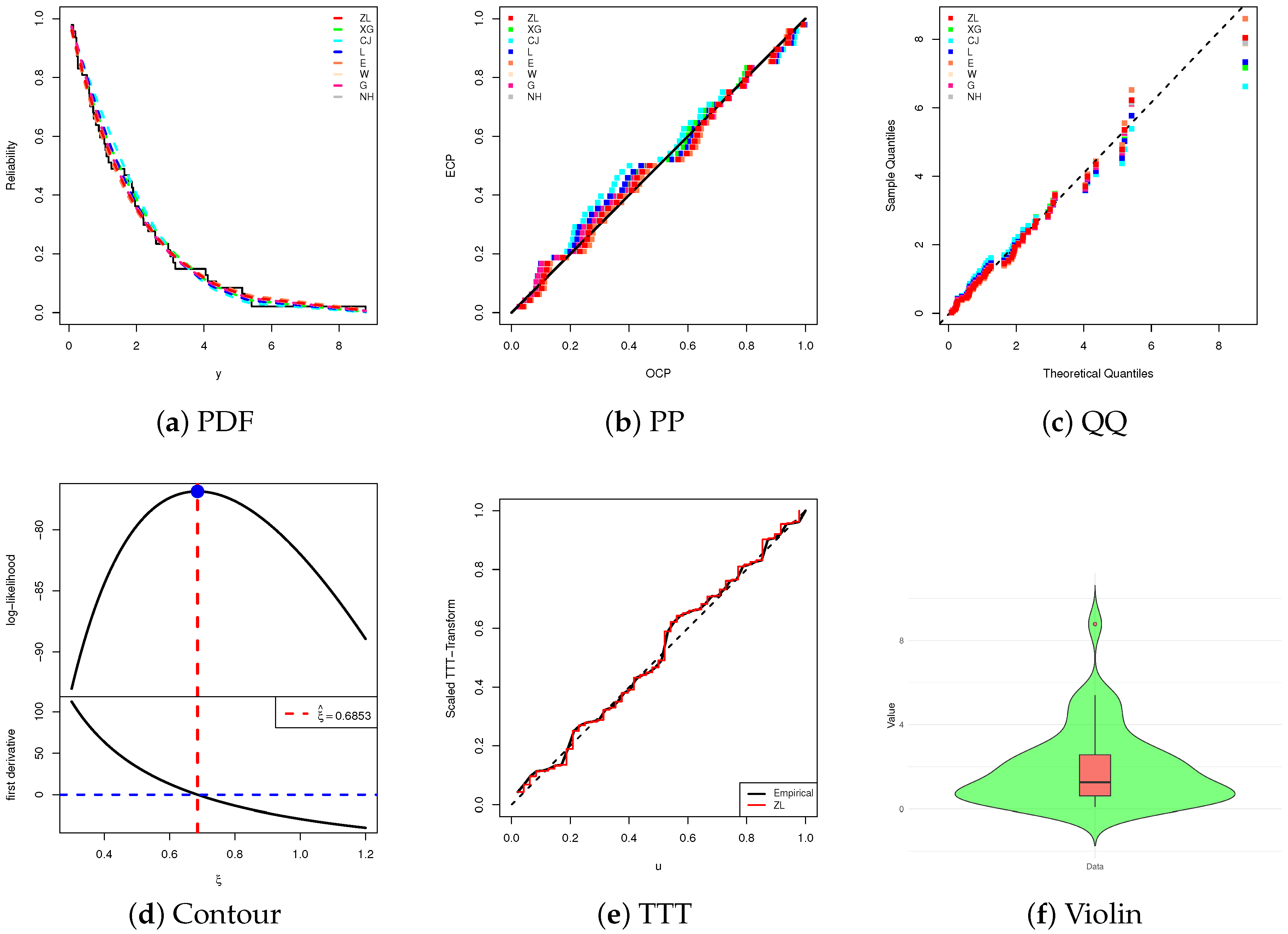
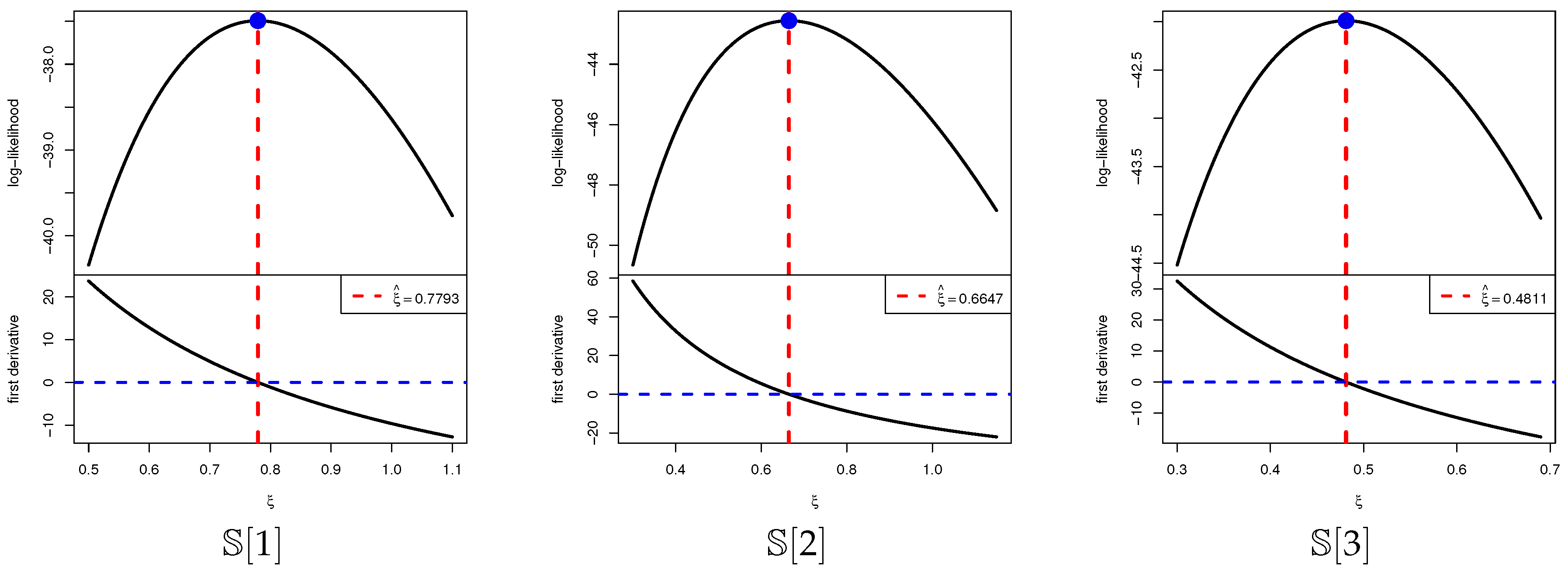
The structure of the paper is as follows: Section 2 and Section 3 develop the frequentist estimations, respectively. Section 4 reports the Monte Carlo results and their interpretations, while Section 5 demonstrates the applicability of the proposed approaches and techniques through two real data analyses. Concluding remarks and final observations are provided in Section 6.

2. Classical Inference

This part considers the estimation of maximum likelihood to carry out both point and interval estimators of $\xi$, $R\left(x\right)$, and $h\left(x\right)$. To achieve this goal, we assume that $\mathbf{y}$ is a T2I-APC sample collected from the proposed ZL population.

2.1. Maximum Likelihood Estimators

This subsection is devoted to deriving the MLEs of the ZL parameters $\xi$, $R\left(x\right)$, and $h\left(x\right)$, denoted by $\widehat{\xi }$, $\widehat{R}\left(x\right)$, and $\widehat{h}\left(x\right)$, respectively. Using (1), (2) and (5), we can re-express the JLF (5) as follows:

$$\begin{array}{c}\hfill \mathcal{L}\left(\xi \right|\mathbf{y})\propto {\overline{\xi }}^{Q_2}{e}^{-\xi \psi }\prod _{i=1}^{Q_2}\left(1+\xi \left(2+y_i\right)\right)\prod _{i=1}^{Q_1}{\left(1+0.5y_i\overline{\xi }\right)}^{S_i}{\left(1+0.5T^{🟉}\overline{\xi }\right)}^{S^{🟉}},\end{array}$$

(6)

where $\overline{\xi }={\displaystyle \frac{\xi }{1+\xi }}$ and $\psi ={\sum }_{i=1}^{Q_2}{y}_i+{\sum }_{i=1}^{Q_1}{y}_i{S}_i+T^{🟉}{S}^{🟉}$.

The corresponding log-JLF of (6) becomes

$$\begin{array}{cc}\hfill log\mathcal{L}\left(\xi \right|\mathbf{y})& \propto Q_{2}log\left(\overline{\xi }\right)-\xi \psi +{\sum }_{i=1}^{Q_2}log\left(1+\xi \left(2+y_i\right)\right)+{\sum }_{i=1}^{Q_1}{S}_{i}log\left(1+0.5y_i\overline{\xi }\right)\hfill \\ \hfill & +S^{🟉}log\left(1+0.5T^{🟉}\overline{\xi }\right).\hfill \end{array}$$

(7)

Thus, the MLE $\widehat{\xi }$ of $\xi$ can be formulated as follows:

$$\begin{array}{c}\hfill \widehat{\Im }\left(\widehat{\xi }\right)=\sqrt{{\displaystyle \frac{Q_2\overline{\xi }}{\psi -{\displaystyle \sum _{i=1}^{Q_2}}{A}_i\left(\xi \right)-0.5{\displaystyle \sum _{i=1}^{Q_1}}{B}_i\left(\xi \right)-0.5C\left(\xi \right)}}}{|}_{\xi =\widehat{\xi }}=0,\end{array}$$

(8)

where

$A_i\left(\xi \right)=\left(2+y_i\right){\left(1+\xi \left(2+y_i\right)\right)}^{-1},$

$B_i\left(\xi \right)={\left({\displaystyle \frac{\overline{\xi }}{\xi }}\right)}^2{y}_i{S}_i{\left(1+0.5y_i\overline{\xi }\right)}^{-1}$

and

$C\left(\xi \right)={\left({\displaystyle \frac{\overline{\xi }}{\xi }}\right)}^2{T}^{🟉}S{\left(1+0.5T^{🟉}\overline{\xi }\right)}^{-1}.$

It is clear that the MLE $\widehat{\xi }$ is obtained by solving the nonlinear likelihood equation given in (8). For this purpose, we employ the Newton–Raphson (NR) iterative scheme. Let $\Im \left(\xi \right)$ denote the score function based on (8), and ${\Im }^{\circ }\left(\xi \right)$ its derivative with respect to $\xi$. Starting from an initial guess ${\xi }^{\left(0\right)}>0$, the iteration proceeds as

$${\xi }^{(k+1)}={\xi }^{\left(k\right)}-{\displaystyle \frac{\Im \left({\xi }^{\left(k\right)}\right)}{{\Im }^{\circ }\left({\xi }^{\left(k\right)}\right)}},k=0,1,2,\dots ,$$

(9)

until convergence is achieved. The process is terminated when either the relative change in successive estimates falls below a prescribed tolerance (e.g., ${10}^{-8}$) or the absolute value of the score function becomes sufficiently small. This iterative approach guarantees a stable and efficient estimation of $\xi$.

It is also important to investigate the existence and uniqueness of the MLE $\widehat{\xi }$. Owing to the complicated structure of the score equation in (8), establishing these properties analytically is not straightforward. To overcome this difficulty, we examine them numerically by generating a T2I-APC sample from the ZL distribution with two different choices of $\xi$, namely $\widehat{\xi }=(0.8,1.5)$, under the setup $n=100$, $r=50$, $({\tau }_1,{\tau }_2)=(1,2)$, and $S_i=1,i=1,2,\dots ,r$. The resulting MLEs of $\xi$ are 0.7458 and 1.2721 for the two cases, respectively. Figure 1 illustrates the log-JLF together with its first and second derivatives. The plot indicates that the vertical line at the MLE intersects the log-JLF at its maximum and the score function at zero. These graphical observations confirm that the MLE of $\xi$ exists and is unique.

Once the estimate $\widehat{\xi }$ is obtained, making use the invariance feature of $\widehat{\xi }$, the MLEs of the reliability $R\left(x\right)$ and hazard rate $h\left(x\right)$ functions, denoted by $\widehat{R}\left(x\right)$ and $\widehat{h}\left(x\right)$, can be directly derived (for $x>0$) as follows:

$$\widehat{R}\left(x\right)=\left[1+0.5x\widehat{\overline{\xi }}\right]e^{-\widehat{\xi }x}\mathrm{and}\widehat{h}\left(x\right)={\displaystyle \frac{\widehat{\xi }(1+\widehat{\xi }(2+x))}{2+\widehat{\xi }(2+x)}},$$

respectively.

2.2. Asymptotic Interval Estimators

Besides obtaining point estimates, it is crucial to construct the $100(1-a)\%$ ACIs for the parameters $\xi$, $R\left(x\right)$, and $h\left(x\right)$. These intervals are derived from the large-sample properties of the MLE $\widehat{\xi }$, which is asymptotically normal with mean $\xi$ and variance–covariance (VC) matrix $\mathbb{V}(·)$. While the theoretical VC matrix is defined through the Fisher information (FI) (say, $\mathbb{I}(·)$), its analytical form is often intractable for the present model. To overcome this difficulty, the VC matrix is approximated by the inverse of the observed FI (OFI) matrix evaluated at the MLE, that is, ${\mathbb{I}(·)|}_{\xi =\widehat{\xi }}$. Hence, the estimated VC matrix can be expressed as:

$$\mathbb{V}\left(\widehat{\xi }\right)={\left[Q_2\left(2\xi +1\right){\overline{\xi }}^2{\xi }^{-4}+{\sum }_{i=1}^{Q_2}{A}_i^{•}\left(\xi \right)+0.5{\sum }_{i=1}^{Q_1}{B}_i^{•}\left(\xi \right)+0.5C^{•}\left(\xi \right)\right]}_{\widehat{\xi }=\xi }^{-1},$$

(10)

where

$A_i^{•}\left(\xi \right)={\left(2+y_i\right)}^2{\left(1+\xi \left(2+y_i\right)\right)}^{-2},$

$B_i^{•}\left(\xi \right)=y_i{S}_i{\left({\displaystyle \frac{\overline{\xi }}{\xi }}\right)}^3{\left(1+0.5y_i\overline{\xi }\right)}^{-1}\left\{1+0.5y_i\left({\displaystyle \frac{\overline{\xi }}{\xi }}\right){\left(1+0.5y_i\overline{\xi }\right)}^{-1}\right\}$

and

$C^{•}\left(\xi \right)=T^{🟉}{S}_i{\left({\displaystyle \frac{\overline{\xi }}{\xi }}\right)}^3{\left(1+0.5T^{🟉}\overline{\xi }\right)}^{-1}\left\{1+0.5T^{🟉}\left({\displaystyle \frac{\overline{\xi }}{\xi }}\right){\left(1+0.5T^{🟉}\overline{\xi }\right)}^{-1}\right\}.$   

For deriving the $100(1-\alpha )\%$ ACIs of the RF $R\left(x\right)$ and HRF $h\left(x\right)$, one must first obtain suitable approximations for the variances of their estimators, $\widehat{R}\left(x\right)$ and $\widehat{h}\left(x\right)$. An effective approach is the delta method, which provides variance estimates denoted by ${\widehat{\mathbb{V}}}_{\widehat{R}}$ and ${\widehat{\mathbb{V}}}_{\widehat{h}}$. As outlined in Greene [10], the delta method ensures that $\widehat{R}\left(x\right)$ can be treated as approximately normal with mean $R\left(x\right)$ and variance ${\widehat{\mathbb{V}}}_{\widehat{R}}$, and likewise, $\widehat{h}\left(x\right)$ is approximately normal with mean $h\left(x\right)$ and variance ${\widehat{\mathbb{V}}}_{\widehat{h}}$. Subsequently, the quantities of ${\widehat{\mathbb{V}}}_{\widehat{R}}$ and ${\widehat{\mathbb{V}}}_{\widehat{h}}$ are given by:

$${\widehat{\mathbb{V}}}_{\widehat{R}}={\left.\mathbb{V}\left(\xi \right){\Lambda }_R^2\right|}_{\xi =\widehat{\xi }}\mathrm{and}{\widehat{\mathbb{V}}}_{\widehat{h}}={\left.\mathbb{V}\left(\xi \right){\Lambda }_h^2\right|}_{\xi =\widehat{\xi }},$$

respectively, where

$${\Lambda }_R=x\left(0.5{\overline{\xi }}^2{\xi }^{-2}-0.5x\overline{\xi }-1\right)e^{-\xi x}$$

and

$${\Lambda }_h={\displaystyle \frac{\xi (x+2)\left[\xi \right(x+2)+4]+2}{{(\xi (x+2)+2)}^2}}.$$

Consequently, the $(1-a)100\%$ ACI based on the normal approximation (say, ACI[NA]) of $\xi$ (at a significance level $a\%$) is given by

$$\widehat{\xi }\mp z_{{\displaystyle \frac{a}{2}}}\sqrt{\mathbb{V}\left(\widehat{\xi }\right)},$$

where $z_{{\displaystyle \frac{a}{2}}}$ is the upper $\left({\displaystyle \frac{a}{2}}\right)$th standard Gaussian percentile point. Similarly, the ACI[NA] estimator of $\widehat{R}\left(x\right)$ or $\widehat{h}\left(x\right)$ can be easily acquired.

A major drawback of the conventional ACI[NA] method is that it can produce lower confidence bounds that fall below zero, even when the parameter of interest is strictly positive. In practice, negative bounds are typically truncated to zero; however, this correction is ad hoc and does not constitute a formal statistical solution. To overcome this drawback and enhance the robustness of interval estimation, Meeker and Escobar [11] proposed the log-transform normal approximation, referred to as ACI[NL]. Accordingly, the $(1-a)100\%$ ACI[NL] for the scale parameter $\xi$ can be expressed as

$$log\left(\widehat{\xi }\right)\mp z_{{\displaystyle \frac{a}{2}}}\sqrt{\mathbb{V}(log\left(\widehat{\xi }\right))},$$

is equivalent to

$$\widehat{\xi }exp\left(\mp {\displaystyle \frac{z_{\frac{a}{2}}}{\widehat{\xi }}}\sqrt{\mathbb{V}\left(\widehat{\xi }\right)}\right).$$

Similarly, the $(1-a)100\%$ ACI[NL] estimator of $\widehat{R}\left(x\right)$ or $\widehat{h}\left(x\right)$ can be easily derived. To obtain the fitted values of the ML estimates as well as the ACI[NA] and ACI[NL] estimators for $\widehat{\xi }$, $\widehat{R}\left(x\right)$, and $\widehat{h}\left(x\right)$, we recommend employing the Newton–Raphson (NR) algorithm, which can be efficiently implemented using the maxLik package in the R environment.

3. Bayesian Inference

In this section, we derive Bayesian point and credible estimates for the ZL parameters $\xi$, $R\left(x\right)$, and $h\left(x\right)$. The Bayesian approach requires explicit specification of prior information and a loss function, both of which strongly influence the resulting inference. Choosing an appropriate prior distribution for an unknown parameter, however, is often a challenging task. As highlighted by Gelman et al. [12], there is no universally accepted rule for selecting priors in Bayesian analysis. Given that the parameter $\xi$ of the ZL model is strictly positive, a gamma prior offers a convenient and widely adopted option. Accordingly, we assume

$$\xi \sim \mathrm{Gamma}(ϵ,\upsilon ),ϵ,\upsilon >0,$$

with prior density

$$\Phi \left(\xi \right)={\displaystyle \frac{{\upsilon }^{ϵ}}{\Gamma \left(ϵ\right)}}{\xi }^{ϵ-1}{e}^{-\upsilon \xi },\xi >0.$$

(11)

From (6) and (11), the posterior PDF (say $\Omega (·)$) of $\xi$ is

$$\begin{array}{ccc}\hfill \Omega \left(\xi \right|\mathbf{y})& \propto & {\left(1+\xi \right)}^{-Q_2}{\xi }^{Q_2+ϵ-1}{e}^{-\xi \left(\psi +\upsilon \right)}\hfill \\ \hfill & \times & {\displaystyle \prod _{i=1}^{Q_2}}\left(1+\xi \left(2+y_i\right)\right){\displaystyle \prod _{i=1}^{Q_1}}{\left(1+0.5y_i\overline{\xi }\right)}^{S_i}{\left(1+0.5T^{🟉}\overline{\xi }\right)}^{S^{🟉}},\hfill \end{array}$$

(12)

where its normalized term (say, $\Theta$) is given by $\Theta ={\int }_0^{\infty }\Phi \left(\xi \right)\times \mathcal{L}\left(\xi \right|\mathbf{y})d\xi .$

It should be emphasized that the squared-error loss (SEL) function is adopted here, as it represents the most commonly employed symmetric loss criterion in Bayesian inference. Nevertheless, the proposed framework can be readily generalized to accommodate alternative loss functions without altering the overall estimation procedure. Given the posterior PDF (12) and the JLF (6), the Bayes estimator of $\xi$, denoted by $\tilde{\xi }$, against the SEL is given by

$$\begin{array}{ccc}\hfill \tilde{\xi }& =& {\Theta }^{-1}{\int }_0^{\infty }{\left(1+\xi \right)}^{-Q_2}{\xi }^{Q_2+ϵ}{e}^{-\xi \left(\psi +\upsilon \right)}\hfill \\ \hfill & \times & {\displaystyle \prod _{i=1}^{Q_2}}\left(1+\xi \left(2+y_i\right)\right){\displaystyle \prod _{i=1}^{Q_1}}{\left(1+0.5y_i\overline{\xi }\right)}^{S_i}{\left(1+0.5T^{🟉}\overline{\xi }\right)}^{S^{🟉}}d\xi .\hfill \end{array}$$

(13)

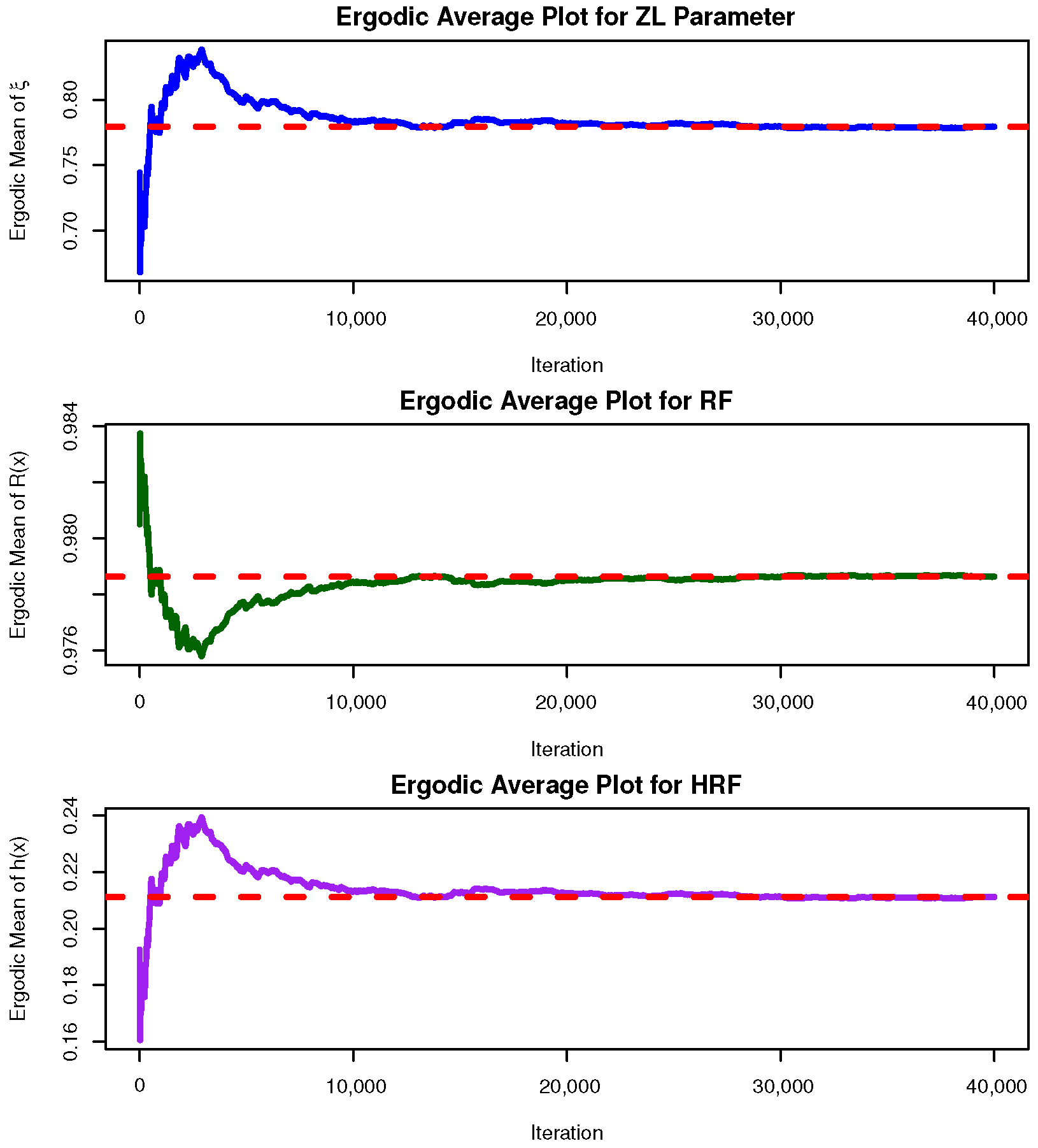
It noted, from (13), that obtaining (closed-form) Bayes estimator of $\xi$, $R\left(x\right)$, or $h\left(x\right)$ under the SEL function is not feasible. To address the analytical intractability of the Bayes estimates, we rely on the Markov chain Monte Carlo (MCMC) procedure to simulate samples from the posterior distribution in (12). These simulated draws enable the computation of Bayesian point estimates together with Bayes credible interval (BCI) and HPD interval estimates for the parameters of interest. 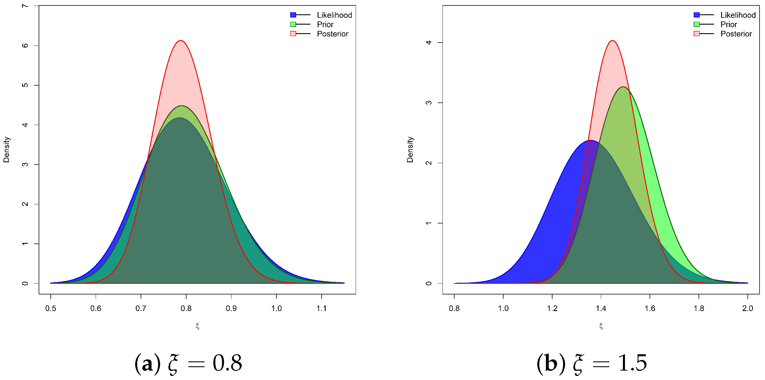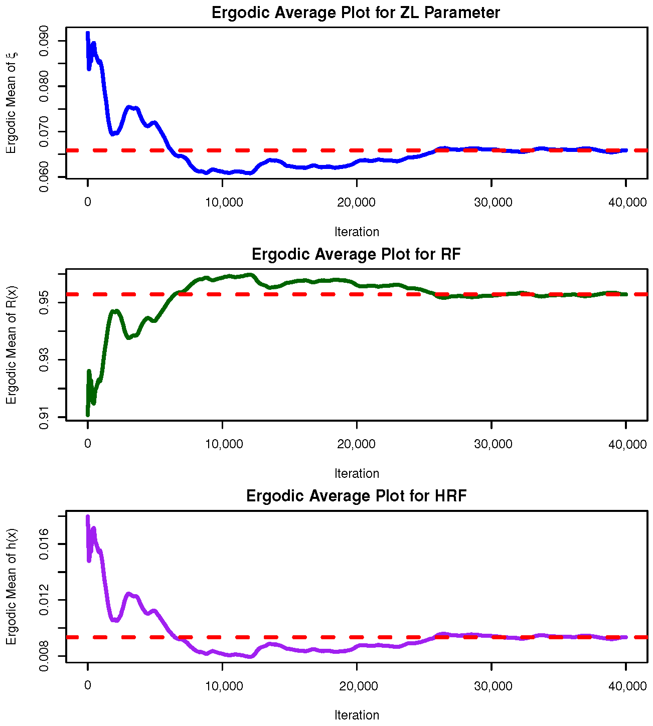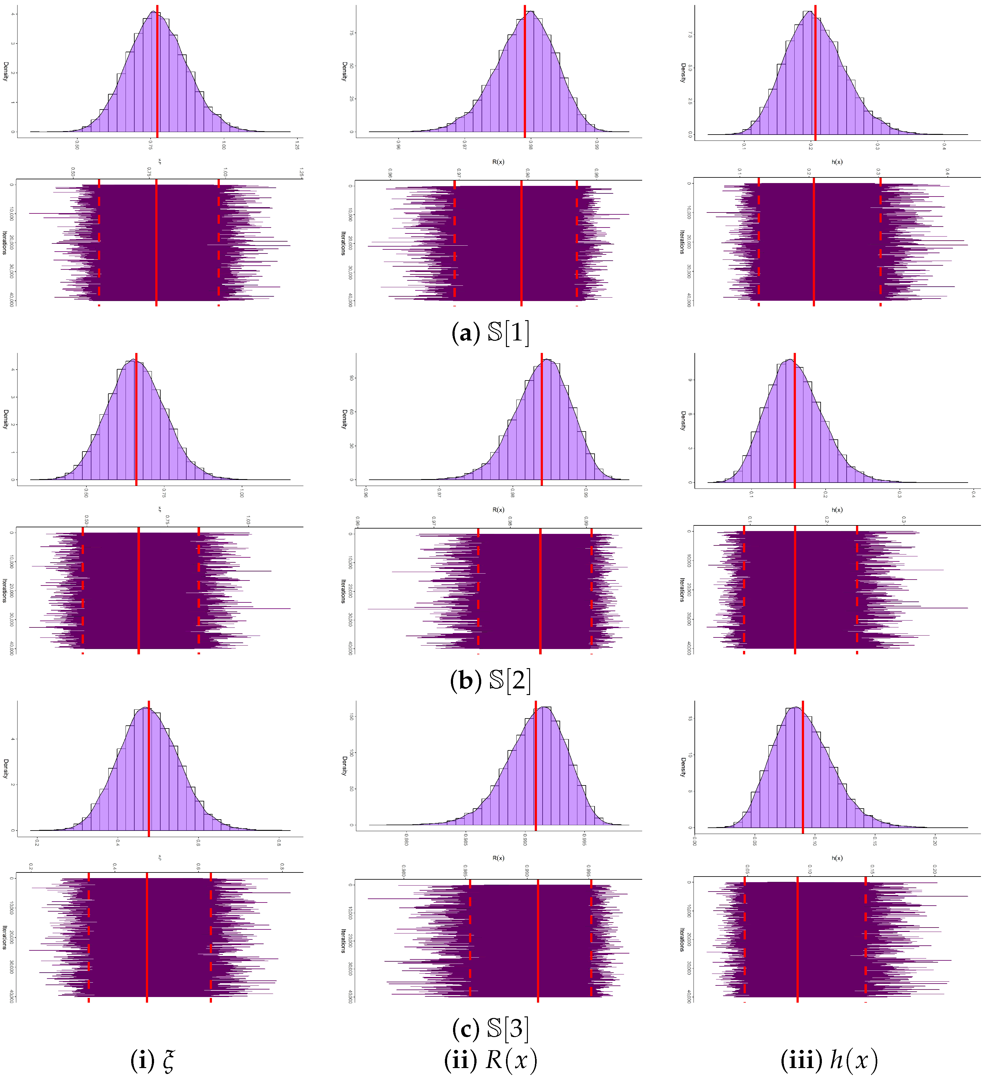Since the posterior density of $\xi$ does not follow any known continuous law, yet resembles a normal distribution as illustrated in Figure 2, the Metropolis–Hastings (M-H) algorithm is adopted to update the posterior draws of $\xi$ (see Algorithm 1). The resulting samples are then employed to evaluate Bayes estimates of $\xi$, $R\left(x\right)$, and $h\left(x\right)$ as well as their corresponding uncertainty measures.

Algorithm 1 The MCMC Steps for Sampling $\xi$, $R\left(x\right)$, and $h\left(x\right)$

1: Input: Initial estimate $\widehat{\xi }$, estimated variance $\widehat{\mathbb{V}}\left(\widehat{\xi }\right)$, total iterations ð, burn-in ${ð}^{\circ }$, confidence level $(1-a)$ 2: Output: Posterior mean $\tilde{\xi }$, BCI and HPD intervals of $\xi$ 3: Put ${\xi }^{\left(0\right)}\leftarrow \widehat{\xi }$ 4: Put $t\leftarrow 1$ 5: while  $t\le ð$  do 6:    Generate ${\xi }^{🟉}\sim N({\xi }^{(t-1)},\widehat{\mathbf{V}}\left(\widehat{\xi }\right))$ 7:    Compute $\aleph \leftarrow min\left(1,{\displaystyle \frac{\Omega ({\xi }^{🟉}\mid \mathbf{y})}{\Omega ({\xi }^{(t-1)}\mid \mathbf{y})}}\right)$ 8:    Generate $u\sim U(0,1)$ 9:    if $u\le \aleph$ then 10:      Put ${\xi }^{\left(t\right)}\leftarrow {\xi }^{🟉}$ 11:    else 12:      Put ${\xi }^{\left(t\right)}\leftarrow {\xi }^{(t-1)}$ 13:    end if 14:    Update $R\left(x\right)$ and $h\left(x\right)$ using ${\xi }^{\left(t\right)}$ in (3) and (4) 15:    Increment $t\leftarrow t+1$ 16: end while 17: Discard the first ${ð}^{\circ }$ samples as burn-in 18: Define ${ð}^{•}=ð-{ð}^{\circ }$ 19: Compute $\tilde{\xi }={\displaystyle \frac{1}{{ð}^{•}}}{\sum }_{t={ð}^{\circ }+1}^{ð}{\xi }^{\left(t\right)}$ 20: Sort ${\xi }^{\left(t\right)}$ for $t={ð}^{\circ }+1,\dots ,ð$ in ascending order 21: Compute the $(1-a)100\%$ BCI of $\xi$ as: $$\left({\xi }_{\left({\displaystyle \frac{a}{2}}{ð}^{•}\right)},{\xi }_{\left(\left(1-{\displaystyle \frac{a}{2}}\right){ð}^{•}\right)}\right)$$ 22: Compute the $(1-a)100\%$ HPD interval of $\xi$ as: $$\left({\xi }_{\left(t^{\odot }\right)},{\xi }_{(t^{\odot }+(1-a){ð}^{•})}\right)$$ where $t^{\odot }$ is the index that minimizes: $${\xi }_{\left(t+(1-a){ð}^{•}\right)}-{\xi }_{\left(t\right)}\mathrm{for}t=1,\dots ,a{ð}^{•}$$ 23: Redo Steps 19–22 for $R\left(x\right)$ and $h\left(x\right)$

4. Monte Carlo Evaluations

To evaluate the accuracy and practical performance of the estimators of $\xi$, $R\left(x\right)$, and $h\left(x\right)$ derived earlier, a series of Monte Carlo simulations were carried out. Using Algorithm 2, the T2I-APC procedure was replicated 1000 times for each of the parameter settings $\xi =0.8$ and $1.5$, yielding estimates of all quantities of interest. At the fixed time point $x=0.1$, the corresponding reliability measures are obtained as $\left(R\right(x),h(x\left)\right)=(0.97797,0.58261)$ for $\xi =0.8$ and $(0.94002,1.20874)$ for $\xi =1.5$. Additional simulations were performed under varying conditions defined by the threshold parameters ${\tau }_i,i=1,2$, the total sample size n, the effective sample size r, and the censoring pattern $\mathbf{S}$. In particular, we considered ${\tau }_1\in \{0.5,1.0\}$, ${\tau }_2\in \{1.0,1.5\}$, and $n\in \{30,50,80\}$.

Table 2. Different plans of $\mathbf{S}=(S_1,S_2,\dots ,S_r)$ in Monte Carlo simulations.

Test	$(\mathit{n},\mathit{r})$	Test	$(\mathit{n},\mathit{r})$
	(30,10)		(30,20)
A1[1]	(5$\times 4$, 0$\times 6$)	A2[1]	(5$\times 2$, 0$\times 18$)
B1[2]	(0$\times 3$, 5$\times 4$, 0$\times 3$)	B2[2]	(0$\times 9$, 5$\times 2$, 0$\times 9$)
C1[3]	(0$\times 6$, 5$\times 4$)	C2[3]	(0$\times 18$, 5$\times 2$)
	(50,20)		(50,40)
A1[1]	(5$\times 6$, 0$\times 14$)	A2[1]	(5$\times 2$, 0$\times 38$)
B1[2]	(0$\times 7$, 5$\times 6$, 0$\times 7$)	B2[2]	(0$\times 19$, 5$\times 2$, 0$\times 19$)
C1[3]	(0$\times 14$, 5$\times 6$)	C2[3]	(0$\times 38$, 5$\times 2$)
	(80,30)		(80,60)
A1[1]	(5$\times 10$, 0$\times 20$)	A2[1]	(5$\times 4$, 0$\times 56$)
B1[2]	(0$\times 10$, 5$\times 10$, 0$\times 10$)	B2[2]	(0$\times 28$, 5$\times 4$, 0$\times 28$)
C1[3]	(0$\times 20$, 5$\times 10$)	C2[3]	(0$\times 56$, 5$\times 4$)

summarizes, for each choice of n, the corresponding values of r along with their associated T2-PC schemes $\mathbf{S}$. For ease of presentation, a notation such as $5^2$ indicates that five units are withdrawn at each of the first two censoring stages.

Algorithm 2 Simulation of T2I-APC Sample.

1: Input: Values of n, r, ${\tau }_i(i=1,2)$, and $\mathbf{S}$. 2: Set the true parameter value of the ZL($\xi$) distribution. 3: Generate r independent random variables ${\varrho }_1,{\varrho }_2,\dots ,{\varrho }_r\sim U(0,1)$. 4: for $i=1$ to r do 5:    Compute ${\displaystyle {\sigma }_i={\varrho }_i^{{\left(i+{\sum }_{j=r-i+1}^r{S}_j\right)}^{-1}}}$. 6: end for 7: for $i=1$ to r do 8:    Compute ${\displaystyle U_i=1-\prod _{j=r-i+1}^r{\sigma }_j}$. 9: end for 10: for $i=1$ to r do 11:    Compute $y_i=G^{-1}(U_i;\xi )$. 12: end for 13: Observe $d_1$ failures at time ${\tau }_1$. 14: Remove observations $y_i$ for $i=d_1+2,\dots ,r$. 15: Set truncated sample size as ${\displaystyle n_{\mathrm{trunc}}=n-d_1-1-{\sum }_{i=1}^{d_1}{S}_i}$. 16: Simulate $y_{d_1+2},\dots ,y_r$ order statistics from the truncated distribution with PDF ${\displaystyle \frac{g\left(y\right)}{R\left(y_{d_1+1}\right)}}$ 17: if  $y_r<{\tau }_1<{\tau }_2$  then 18:    Case 1: Stop the test at $y_r$. 19: else if  ${\tau }_1<y_r<{\tau }_2$ then 20:    Case 2: Stop the test at $y_r$. 21: else if  ${\tau }_1<{\tau }_2<y_r$ then 22:    Case 3: Stop the test at ${\tau }_2$. 23: end if

Once 1000 T2I-APC datasets are generated, the frequentist estimates along with their corresponding 95% asymptotic confidence intervals (ACI-NA and ACI-NL) for $\xi$, $R\left(x\right)$, and $h\left(x\right)$ are obtained using the maxLik package (Henningsen and Toomet [13]) in the R environment (version 4.2.2).

For the Bayesian analysis, we generate $ð=\mathrm{12,000}$ MCMC samples, discarding the first ${ð}^{\circ }=2000$ iterations as burn-in. The Bayesian posterior estimates, together with their 95% BCI/HPD intervals for $\xi$, $R\left(x\right)$, and $h\left(x\right)$, are computed using the coda package (Plummer et al. [14]) in the same R environment.

To further assess the sensitivity of the proposed Bayesian estimation procedures, two distinct sets of hyperparameters $(ϵ,\upsilon )$ were examined. Following the prior elicitation strategy of Kundu [15], the hyperparameters of the gamma prior distribution were specified as follows: Prior-A = $(4,5)$ and Prior-B = $(8,10)$ for $\xi =0.8$, and Prior-A = $(7.5,5)$ and Prior-B = $(15,10)$ for $\xi =1.5$. The hyperparameter values of $ϵ$ and $\upsilon$ for the ZL parameter $\xi$ were selected such that the resulting prior means corresponded to plausible values of $\xi$. Notably, Prior-A represents a diffuse prior with larger variance, reflecting minimal prior information, whereas Prior-B corresponds to a more concentrated prior informed by empirical knowledge of the ZLindley model’s scale range. Simulation evidence revealed that, although both priors produced consistent posterior means, Prior-B yielded smaller posterior variances, narrower HPD intervals, and improved coverage probabilities, highlighting the stabilizing influence of informative priors without introducing substantial bias.

To evaluate the performance of the ZL parameter estimators of $\xi$, $R\left(x\right)$, and $h\left(x\right)$, we compute the following summary metrics:

• Mean Point Estimate: $\mathrm{MPE}\left(\widehat{\xi }\right)={\displaystyle \frac{1}{1000}}{\sum }_{i=1}^{1000}{\widehat{\xi }}^{\left[i\right]};$
• Root Mean Squared Error: $\mathrm{RMSE}\left(\widehat{\xi }\right)=\sqrt{{\displaystyle \frac{1}{1000}}{\sum }_{i=1}^{1000}{\left({\widehat{\xi }}^{\left[i\right]}-\xi \right)}^2};$
• Average Relative Absolute Bias: $\mathrm{ARAB}\left(\widehat{\xi }\right)={\displaystyle \frac{1}{1000}}{\sum }_{i=1}^{1000}{\widehat{\xi }}^{-1}\left|{\widehat{\xi }}^{\left[i\right]}-\xi \right|;$
• Average Interval Length: ${\mathrm{AIL}}_{95\%}\left(\xi \right)={\displaystyle \frac{1}{1000}}{\sum }_{i=1}^{1000}\left({\mathsf{U}}_{{\widehat{\xi }}^{\left[i\right]}}-{\mathsf{L}}_{{\widehat{\xi }}^{\left[i\right]}}\right);$
• Coverage Probability: ${\mathrm{CP}}_{95\%}\left(\xi \right)={\displaystyle \frac{1}{1000}}{\sum }_{i=1}^{1000}{\Xi }_{({\mathsf{L}}_{{\widehat{\xi }}^{\left[i\right]}},{\mathsf{U}}_{{\widehat{\xi }}^{\left[i\right]}})}\left(\xi \right),$ where ${\widehat{\xi }}^{\left[i\right]}$ denotes the ith point estimate of $\xi$ and $\Xi (·)$ is the indicator function. The same precision metrics are also applied to the estimates of $R\left(x\right)$ and $h\left(x\right)$.

From

Table 3. Point estimation results of $\xi$.

$(\mathit{n},\mathit{r})$	Design	MLE			Bayesian						MLE			Bayesian
Prior→					A			B						A			B
		$({\mathbf{\tau }}_{\mathbf{1}},{\mathbf{\tau }}_{\mathbf{2}})=(\mathbf{0.5},\mathbf{1.0})$									$({\mathbf{\tau }}_{\mathbf{1}},{\mathbf{\tau }}_{\mathbf{2}})=(\mathbf{1.0},\mathbf{1.5})$
		MPE	RMSE	ARAB	MPE	RMSE	ARAB	MPE	RMSE	ARAB	MPE	RMSE	ARAB	MPE	RMSE	ARAB	MPE	RMSE	ARAB
For $\xi =0.8$
(30,10)	A1[1]	0.757	0.377	0.395	0.829	0.086	0.090	0.792	0.080	0.089	0.820	0.269	0.248	0.835	0.085	0.089	0.799	0.070	0.078
	B1[2]	0.766	0.476	0.519	0.834	0.105	0.101	0.796	0.085	0.089	0.805	0.304	0.258	0.833	0.086	0.098	0.795	0.073	0.082
	C1[3]	1.030	0.319	0.340	0.836	0.086	0.089	0.799	0.075	0.083	0.929	0.238	0.233	0.835	0.083	0.086	0.797	0.069	0.076
(30,20)	A2[1]	0.763	0.262	0.277	0.815	0.083	0.086	0.863	0.073	0.074	0.779	0.237	0.228	0.811	0.074	0.083	0.858	0.068	0.071
	B2[2]	0.712	0.232	0.231	0.808	0.079	0.079	0.854	0.071	0.073	0.785	0.225	0.224	0.816	0.073	0.076	0.864	0.068	0.071
	C2[3]	0.713	0.206	0.219	0.811	0.076	0.076	0.858	0.066	0.071	0.828	0.175	0.177	0.811	0.069	0.073	0.858	0.059	0.066
(50,20)	A1[1]	0.720	0.184	0.187	0.811	0.069	0.076	0.856	0.060	0.067	0.798	0.171	0.175	0.816	0.065	0.068	0.864	0.058	0.065
	B1[2]	0.770	0.186	0.196	0.812	0.069	0.076	0.859	0.065	0.069	0.786	0.175	0.176	0.814	0.068	0.072	0.860	0.059	0.065
	C1[3]	0.824	0.181	0.183	0.803	0.067	0.074	0.843	0.058	0.065	0.924	0.168	0.171	0.823	0.060	0.065	0.869	0.057	0.059
(50,40)	A2[1]	0.775	0.173	0.181	0.759	0.059	0.065	0.841	0.050	0.052	0.785	0.166	0.165	0.756	0.058	0.065	0.833	0.050	0.050
	B2[2]	0.740	0.147	0.148	0.756	0.059	0.065	0.833	0.049	0.050	0.780	0.137	0.136	0.759	0.057	0.065	0.836	0.048	0.050
	C2[3]	0.754	0.146	0.141	0.756	0.059	0.065	0.833	0.048	0.048	0.765	0.132	0.132	0.757	0.057	0.064	0.830	0.046	0.048
(80,30)	A1[1]	0.722	0.124	0.123	0.746	0.055	0.061	0.852	0.045	0.046	0.797	0.113	0.109	0.753	0.055	0.061	0.858	0.045	0.046
	B1[2]	0.779	0.131	0.130	0.750	0.057	0.063	0.859	0.046	0.047	0.793	0.130	0.129	0.753	0.055	0.062	0.861	0.045	0.046
	C1[3]	0.743	0.112	0.109	0.728	0.055	0.061	0.834	0.045	0.046	0.882	0.107	0.105	0.770	0.055	0.061	0.880	0.043	0.045
(80,60)	A2[1]	0.781	0.109	0.109	0.760	0.055	0.060	0.791	0.042	0.045	0.787	0.104	0.103	0.758	0.054	0.060	0.787	0.041	0.045
	B2[2]	0.729	0.102	0.103	0.754	0.054	0.058	0.783	0.041	0.045	0.786	0.100	0.101	0.757	0.053	0.058	0.783	0.041	0.044
	C2[3]	0.754	0.090	0.088	0.758	0.053	0.056	0.786	0.041	0.044	0.761	0.082	0.081	0.754	0.053	0.056	0.780	0.041	0.044
For $\xi =1.5$
(30,10)	A1[1]	1.489	0.539	0.330	1.535	0.089	0.049	1.497	0.079	0.048	1.545	0.510	0.242	1.535	0.088	0.049	1.497	0.078	0.047
	B1[2]	1.452	0.774	0.427	1.534	0.095	0.052	1.496	0.087	0.048	1.507	0.574	0.342	1.535	0.088	0.051	1.497	0.078	0.047
	C1[3]	1.769	0.494	0.237	1.535	0.086	0.047	1.497	0.077	0.046	1.634	0.425	0.232	1.535	0.078	0.047	1.497	0.076	0.042
(30,20)	A2[1]	1.432	0.472	0.227	1.517	0.077	0.046	1.566	0.076	0.039	1.473	0.418	0.209	1.517	0.077	0.046	1.565	0.076	0.039
	B2[2]	1.425	0.457	0.223	1.517	0.077	0.046	1.565	0.076	0.039	1.485	0.395	0.200	1.517	0.076	0.045	1.566	0.076	0.039
	C2[3]	1.884	0.396	0.202	1.526	0.076	0.045	1.575	0.073	0.038	1.754	0.334	0.181	1.519	0.076	0.045	1.567	0.066	0.035
(50,20)	A1[1]	1.462	0.305	0.158	1.517	0.071	0.043	1.565	0.059	0.035	1.490	0.290	0.154	1.517	0.071	0.043	1.566	0.059	0.035
	B1[2]	1.442	0.323	0.162	1.517	0.076	0.045	1.565	0.059	0.035	1.475	0.308	0.160	1.518	0.071	0.043	1.566	0.059	0.035
	C1[3]	1.817	0.303	0.156	1.519	0.071	0.043	1.567	0.059	0.035	1.566	0.271	0.153	1.519	0.071	0.043	1.567	0.058	0.035
(50,40)	A2[1]	1.456	0.296	0.154	1.456	0.060	0.036	1.539	0.057	0.034	1.470	0.270	0.144	1.455	0.059	0.035	1.536	0.049	0.027
	B2[2]	1.425	0.296	0.154	1.454	0.059	0.035	1.536	0.056	0.029	1.472	0.269	0.143	1.455	0.057	0.034	1.536	0.049	0.026
	C2[3]	1.380	0.244	0.128	1.449	0.058	0.034	1.528	0.049	0.026	1.893	0.243	0.124	1.467	0.057	0.034	1.553	0.048	0.026
(80,30)	A1[1]	1.468	0.230	0.119	1.452	0.055	0.033	1.564	0.048	0.026	1.485	0.229	0.119	1.452	0.055	0.032	1.564	0.046	0.025
	B1[2]	1.466	0.237	0.126	1.452	0.057	0.034	1.564	0.048	0.026	1.476	0.232	0.121	1.452	0.055	0.033	1.564	0.047	0.025
	C1[3]	1.736	0.222	0.116	1.461	0.055	0.033	1.574	0.046	0.025	1.543	0.206	0.108	1.453	0.055	0.032	1.564	0.043	0.024
(80,60)	A2[1]	1.471	0.204	0.108	1.460	0.055	0.032	1.491	0.046	0.025	1.482	0.193	0.101	1.459	0.054	0.031	1.491	0.041	0.024
	B2[2]	1.458	0.193	0.097	1.452	0.055	0.032	1.485	0.041	0.023	1.485	0.164	0.087	1.459	0.054	0.030	1.490	0.041	0.023
	C2[3]	1.380	0.164	0.087	1.453	0.053	0.030	1.484	0.040	0.023	1.938	0.155	0.082	1.476	0.052	0.028	1.517	0.040	0.023

,

Table 4. Point estimation results of $R\left(x\right)$.

$(\mathit{n},\mathit{r})$	Design	MLE			Bayesian						MLE			Bayesian
Prior→					A			B						A			B
		$({\mathbf{\tau }}_{\mathbf{1}},{\mathbf{\tau }}_{\mathbf{2}})=(\mathbf{0.5},\mathbf{1.0})$									$({\mathbf{\tau }}_{\mathbf{1}},{\mathbf{\tau }}_{\mathbf{2}})=(\mathbf{1.0},\mathbf{1.5})$
		MPE	RMSE	ARAB	MPE	RMSE	ARAB	MPE	RMSE	ARAB	MPE	RMSE	ARAB	MPE	RMSE	ARAB	MPE	RMSE	ARAB
For $\xi =0.8$
(30,10)	A1[1]	0.965	0.474	0.388	0.976	0.115	0.098	0.978	0.107	0.095	0.971	0.352	0.278	0.976	0.111	0.097	0.978	0.099	0.089
	B1[2]	0.979	0.752	0.644	0.976	0.137	0.117	0.978	0.115	0.098	0.977	0.480	0.312	0.976	0.122	0.106	0.978	0.105	0.095
	C1[3]	0.979	0.582	0.468	0.977	0.115	0.104	0.978	0.114	0.097	0.976	0.419	0.302	0.976	0.114	0.098	0.978	0.100	0.090
(30,20)	A2[1]	0.982	0.273	0.237	0.977	0.101	0.089	0.975	0.094	0.081	0.976	0.250	0.207	0.977	0.099	0.082	0.975	0.082	0.075
	B2[2]	0.981	0.336	0.259	0.978	0.105	0.092	0.975	0.097	0.083	0.978	0.317	0.254	0.977	0.101	0.085	0.975	0.097	0.078
	C2[3]	0.979	0.367	0.308	0.977	0.111	0.096	0.975	0.098	0.086	0.978	0.349	0.261	0.977	0.106	0.095	0.975	0.097	0.078
(50,20)	A1[1]	0.975	0.242	0.202	0.978	0.096	0.085	0.976	0.082	0.074	0.972	0.234	0.191	0.977	0.083	0.074	0.975	0.081	0.068
	B1[2]	0.979	0.246	0.213	0.977	0.099	0.089	0.975	0.092	0.080	0.978	0.240	0.197	0.977	0.093	0.080	0.975	0.081	0.074
	C1[3]	0.981	0.246	0.205	0.977	0.098	0.088	0.975	0.083	0.076	0.978	0.238	0.195	0.977	0.092	0.079	0.975	0.081	0.074
(50,40)	A2[1]	0.980	0.186	0.150	0.980	0.081	0.074	0.976	0.066	0.055	0.979	0.185	0.147	0.980	0.078	0.071	0.977	0.065	0.055
	B2[2]	0.981	0.197	0.164	0.980	0.082	0.074	0.976	0.069	0.057	0.979	0.191	0.153	0.980	0.080	0.073	0.976	0.067	0.056
	C2[3]	0.979	0.232	0.197	0.980	0.082	0.074	0.976	0.069	0.059	0.978	0.229	0.187	0.980	0.081	0.073	0.976	0.068	0.057
(80,30)	A1[1]	0.979	0.147	0.118	0.981	0.077	0.070	0.976	0.062	0.051	0.974	0.145	0.117	0.979	0.077	0.070	0.974	0.061	0.051
	B1[2]	0.979	0.178	0.147	0.980	0.078	0.071	0.975	0.063	0.053	0.978	0.174	0.143	0.980	0.078	0.070	0.975	0.063	0.053
	C1[3]	0.981	0.169	0.138	0.980	0.078	0.070	0.976	0.063	0.053	0.978	0.147	0.121	0.980	0.077	0.070	0.975	0.063	0.053
(80,60)	A2[1]	0.980	0.119	0.097	0.980	0.072	0.062	0.979	0.056	0.050	0.980	0.110	0.089	0.980	0.072	0.062	0.979	0.056	0.050
	B2[2]	0.981	0.139	0.113	0.980	0.074	0.064	0.979	0.056	0.050	0.978	0.132	0.112	0.980	0.073	0.064	0.979	0.056	0.050
	C2[3]	0.979	0.146	0.118	0.980	0.075	0.069	0.978	0.057	0.050	0.978	0.140	0.113	0.980	0.074	0.067	0.979	0.056	0.050
For $\xi =1.5$
(30,10)	A1[1]	0.923	0.893	0.697	0.938	0.153	0.136	0.940	0.140	0.133	0.931	0.798	0.689	0.938	0.142	0.135	0.940	0.136	0.121
	B1[2]	0.942	1.177	0.975	0.938	0.169	0.150	0.940	0.157	0.138	0.939	1.083	1.020	0.938	0.158	0.146	0.940	0.142	0.136
	C1[3]	0.940	0.992	0.863	0.938	0.158	0.143	0.940	0.144	0.138	0.936	0.970	0.723	0.938	0.157	0.139	0.940	0.142	0.136
(30,20)	A2[1]	0.915	0.745	0.602	0.938	0.137	0.131	0.935	0.131	0.108	0.924	0.623	0.536	0.939	0.137	0.131	0.936	0.117	0.102
	B2[2]	0.944	0.843	0.640	0.939	0.140	0.133	0.936	0.136	0.111	0.940	0.711	0.566	0.939	0.137	0.131	0.936	0.135	0.111
	C2[3]	0.944	0.879	0.659	0.939	0.140	0.133	0.936	0.136	0.111	0.941	0.759	0.596	0.939	0.140	0.133	0.936	0.136	0.111
(50,20)	A1[1]	0.920	0.551	0.446	0.939	0.130	0.125	0.936	0.106	0.102	0.936	0.494	0.436	0.939	0.130	0.125	0.936	0.105	0.100
	B1[2]	0.943	0.598	0.472	0.939	0.137	0.131	0.936	0.106	0.102	0.941	0.537	0.449	0.939	0.130	0.125	0.936	0.106	0.102
	C1[3]	0.942	0.557	0.453	0.939	0.130	0.125	0.936	0.106	0.102	0.940	0.518	0.438	0.939	0.130	0.125	0.936	0.106	0.102
(50,40)	A2[1]	0.947	0.447	0.361	0.943	0.103	0.099	0.938	0.088	0.076	0.915	0.426	0.359	0.942	0.103	0.099	0.937	0.086	0.076
	B2[2]	0.944	0.535	0.439	0.943	0.105	0.100	0.938	0.102	0.084	0.941	0.472	0.404	0.943	0.103	0.099	0.938	0.088	0.076
	C2[3]	0.942	0.536	0.442	0.943	0.108	0.103	0.938	0.103	0.099	0.942	0.477	0.409	0.943	0.106	0.100	0.938	0.088	0.077
(80,30)	A1[1]	0.925	0.397	0.332	0.942	0.100	0.095	0.936	0.083	0.074	0.937	0.369	0.309	0.943	0.100	0.094	0.936	0.078	0.069
	B1[2]	0.942	0.426	0.357	0.943	0.103	0.097	0.936	0.087	0.075	0.941	0.420	0.347	0.943	0.100	0.094	0.936	0.084	0.073
	C1[3]	0.942	0.413	0.342	0.943	0.100	0.097	0.936	0.086	0.075	0.941	0.413	0.340	0.943	0.100	0.094	0.936	0.083	0.073
(80,60)	A2[1]	0.947	0.295	0.249	0.943	0.095	0.085	0.941	0.072	0.067	0.912	0.276	0.233	0.941	0.092	0.081	0.939	0.072	0.066
	B2[2]	0.942	0.339	0.276	0.943	0.100	0.094	0.941	0.073	0.067	0.941	0.295	0.250	0.942	0.096	0.086	0.941	0.073	0.067
	C2[3]	0.942	0.366	0.309	0.942	0.100	0.094	0.941	0.083	0.073	0.941	0.342	0.288	0.942	0.097	0.088	0.941	0.074	0.068

,

Table 5. Point estimation results of $h\left(x\right)$.

$(\mathit{n},\mathit{r})$	Design	MLE			Bayesian						MLE			Bayesian
Prior→					A			B						A			B
		$({\mathbf{\tau }}_{\mathbf{1}},{\mathbf{\tau }}_{\mathbf{2}})=(\mathbf{0.5},\mathbf{1.0})$									$({\mathbf{\tau }}_{\mathbf{1}},{\mathbf{\tau }}_{\mathbf{2}})=(\mathbf{1.0},\mathbf{1.5})$
		MPE	RMSE	ARAB	MPE	RMSE	ARAB	MPE	RMSE	ARAB	MPE	RMSE	ARAB	MPE	RMSE	ARAB	MPE	RMSE	ARAB
For $\xi =0.8$
(30,10)	A1[1]	0.552	0.331	0.468	0.608	0.073	0.106	0.576	0.069	0.103	0.604	0.237	0.296	0.613	0.072	0.103	0.582	0.060	0.091
	B1[2]	0.559	0.422	0.624	0.612	0.088	0.119	0.580	0.073	0.103	0.591	0.269	0.308	0.611	0.073	0.113	0.578	0.063	0.096
	C1[3]	0.794	0.277	0.398	0.614	0.073	0.103	0.582	0.064	0.098	0.698	0.206	0.276	0.613	0.070	0.100	0.581	0.060	0.090
(30,20)	A2[1]	0.554	0.223	0.322	0.596	0.070	0.100	0.637	0.062	0.087	0.568	0.206	0.268	0.592	0.064	0.098	0.633	0.058	0.083
	B2[2]	0.511	0.196	0.268	0.590	0.067	0.093	0.629	0.061	0.086	0.572	0.196	0.263	0.597	0.062	0.088	0.638	0.058	0.083
	C2[3]	0.510	0.173	0.253	0.593	0.064	0.090	0.633	0.057	0.083	0.613	0.148	0.208	0.593	0.060	0.085	0.632	0.051	0.077
(50,20)	A1[1]	0.518	0.155	0.217	0.592	0.059	0.089	0.631	0.051	0.078	0.583	0.148	0.203	0.597	0.056	0.080	0.638	0.050	0.076
	B1[2]	0.560	0.156	0.226	0.593	0.059	0.090	0.634	0.056	0.081	0.573	0.148	0.206	0.595	0.058	0.084	0.635	0.050	0.076
	C1[3]	0.613	0.152	0.212	0.585	0.058	0.087	0.619	0.050	0.076	0.692	0.143	0.199	0.602	0.051	0.076	0.642	0.049	0.069
(50,40)	A2[1]	0.563	0.145	0.209	0.549	0.050	0.076	0.617	0.042	0.061	0.571	0.142	0.193	0.546	0.050	0.076	0.611	0.042	0.059
	B2[2]	0.532	0.124	0.172	0.546	0.050	0.076	0.611	0.042	0.059	0.567	0.117	0.159	0.549	0.049	0.076	0.614	0.042	0.058
	C2[3]	0.545	0.121	0.162	0.546	0.050	0.076	0.611	0.040	0.057	0.554	0.113	0.154	0.547	0.048	0.074	0.608	0.039	0.056
(80,30)	A1[1]	0.519	0.105	0.144	0.538	0.047	0.072	0.627	0.038	0.054	0.581	0.094	0.126	0.543	0.047	0.072	0.633	0.038	0.054
	B1[2]	0.567	0.111	0.152	0.541	0.048	0.074	0.633	0.039	0.055	0.578	0.110	0.150	0.543	0.048	0.073	0.635	0.038	0.054
	C1[3]	0.541	0.094	0.126	0.522	0.047	0.072	0.612	0.038	0.053	0.655	0.090	0.122	0.557	0.047	0.071	0.652	0.037	0.053
(80,60)	A2[1]	0.523	0.086	0.119	0.544	0.046	0.067	0.568	0.035	0.052	0.572	0.084	0.118	0.546	0.046	0.067	0.568	0.035	0.052
	B2[2]	0.567	0.092	0.126	0.549	0.046	0.070	0.575	0.035	0.052	0.573	0.088	0.119	0.547	0.046	0.070	0.571	0.035	0.052
	C2[3]	0.545	0.076	0.102	0.547	0.045	0.065	0.571	0.035	0.052	0.550	0.069	0.093	0.544	0.045	0.065	0.566	0.035	0.051
For $\xi =1.5$
(30,10)	A1[1]	1.203	0.507	0.384	1.241	0.082	0.057	1.206	0.073	0.055	1.256	0.482	0.282	1.241	0.081	0.056	1.206	0.073	0.054
	B1[2]	1.169	0.733	0.497	1.240	0.087	0.060	1.205	0.081	0.055	1.221	0.540	0.398	1.241	0.080	0.059	1.206	0.072	0.052
	C1[3]	1.464	0.466	0.275	1.241	0.079	0.054	1.206	0.071	0.053	1.339	0.399	0.269	1.241	0.073	0.054	1.206	0.071	0.049
(30,20)	A2[1]	1.148	0.443	0.262	1.225	0.071	0.053	1.270	0.070	0.045	1.186	0.388	0.239	1.225	0.071	0.053	1.269	0.070	0.045
	B2[2]	1.143	0.427	0.256	1.225	0.071	0.053	1.269	0.070	0.045	1.198	0.366	0.228	1.225	0.071	0.052	1.270	0.070	0.043
	C2[3]	1.577	0.372	0.235	1.233	0.070	0.052	1.278	0.068	0.043	1.447	0.313	0.210	1.226	0.070	0.051	1.271	0.061	0.042
(50,20)	A1[1]	1.176	0.284	0.181	1.225	0.066	0.049	1.269	0.054	0.040	1.202	0.267	0.176	1.225	0.066	0.049	1.270	0.054	0.040
	B1[2]	1.158	0.301	0.187	1.225	0.070	0.052	1.269	0.054	0.040	1.188	0.282	0.182	1.225	0.066	0.048	1.270	0.054	0.040
	C1[3]	1.506	0.281	0.178	1.226	0.066	0.049	1.271	0.054	0.040	1.273	0.252	0.175	1.226	0.066	0.049	1.271	0.054	0.041
(50,40)	A2[1]	1.170	0.274	0.177	1.169	0.055	0.041	1.245	0.053	0.040	1.182	0.248	0.165	1.167	0.054	0.040	1.242	0.045	0.031
	B2[2]	1.141	0.274	0.176	1.167	0.054	0.040	1.242	0.052	0.033	1.185	0.246	0.163	1.167	0.053	0.040	1.242	0.044	0.031
	C2[3]	1.099	0.226	0.146	1.162	0.053	0.040	1.235	0.045	0.030	1.580	0.223	0.142	1.178	0.053	0.040	1.258	0.044	0.030
(80,30)	A1[1]	1.181	0.213	0.137	1.164	0.051	0.038	1.268	0.044	0.030	1.196	0.212	0.136	1.164	0.051	0.037	1.268	0.042	0.029
	B1[2]	1.179	0.219	0.144	1.164	0.053	0.039	1.268	0.045	0.030	1.189	0.215	0.139	1.164	0.051	0.037	1.268	0.043	0.029
	C1[3]	1.430	0.205	0.133	1.172	0.051	0.038	1.277	0.043	0.029	1.250	0.190	0.124	1.166	0.051	0.037	1.269	0.040	0.027
(80,60)	A2[1]	1.171	0.177	0.111	1.164	0.051	0.037	1.195	0.038	0.027	1.196	0.152	0.100	1.171	0.049	0.035	1.200	0.038	0.027
	B2[2]	1.182	0.189	0.124	1.172	0.051	0.037	1.201	0.042	0.029	1.193	0.177	0.116	1.171	0.050	0.035	1.201	0.038	0.027
	C2[3]	1.100	0.151	0.100	1.165	0.049	0.034	1.194	0.037	0.027	1.621	0.143	0.093	1.186	0.048	0.032	1.224	0.037	0.026

,

Table 6. Interval estimation results of $\xi$.

$({\mathit{t}}_1,{\mathit{t}}_2)$	$(\mathit{n},\mathit{r})$	Design	ACI-NA		ACI-NL		BCI				HPD
Prior→							A		B		A		B
			AIL	CP	AIL	CP	AIL	CP	AIL	CP	AIL	CP	AIL	CP
For $\xi =0.8$
(0.5,1.0)	(30,10)	A1[1]	1.043	0.927	1.147	0.924	0.442	0.948	0.319	0.960	0.209	0.971	0.165	0.975
		B1[2]	1.092	0.925	1.186	0.923	0.448	0.947	0.326	0.959	0.221	0.969	0.168	0.975
		C1[3]	0.960	0.929	1.016	0.927	0.428	0.949	0.308	0.961	0.209	0.971	0.165	0.975
	(30,20)	A2[1]	0.781	0.933	0.883	0.931	0.424	0.949	0.303	0.961	0.203	0.971	0.157	0.976
		B2[2]	0.755	0.934	0.828	0.932	0.413	0.950	0.299	0.962	0.203	0.971	0.157	0.976
		C2[3]	0.701	0.935	0.724	0.935	0.409	0.951	0.299	0.962	0.202	0.971	0.155	0.976
	(50,20)	A1[1]	0.664	0.936	0.696	0.936	0.401	0.952	0.289	0.963	0.196	0.972	0.155	0.976
		B1[2]	0.680	0.936	0.718	0.935	0.406	0.951	0.294	0.962	0.199	0.972	0.155	0.976
		C1[3]	0.662	0.936	0.683	0.936	0.401	0.952	0.288	0.963	0.194	0.972	0.152	0.976
	(50,40)	A2[1]	0.611	0.938	0.659	0.937	0.396	0.952	0.285	0.963	0.193	0.972	0.152	0.976
		B2[2]	0.560	0.939	0.627	0.937	0.393	0.952	0.284	0.963	0.193	0.972	0.151	0.976
		C2[3]	0.545	0.940	0.554	0.939	0.393	0.952	0.282	0.963	0.190	0.973	0.150	0.976
	(80,30)	A1[1]	0.516	0.940	0.534	0.940	0.377	0.954	0.268	0.965	0.179	0.974	0.139	0.978
		B1[2]	0.539	0.940	0.550	0.939	0.377	0.954	0.274	0.964	0.182	0.973	0.144	0.977
		C1[3]	0.480	0.941	0.511	0.940	0.370	0.955	0.261	0.965	0.175	0.974	0.137	0.978
	(80,60)	A2[1]	0.447	0.942	0.478	0.941	0.347	0.957	0.250	0.967	0.150	0.977	0.118	0.980
		B2[2]	0.418	0.943	0.429	0.943	0.340	0.958	0.246	0.967	0.148	0.977	0.116	0.980
		C2[3]	0.374	0.944	0.427	0.943	0.331	0.959	0.240	0.968	0.144	0.977	0.114	0.980
(1.0,1.5)	(30,10)	A1[1]	0.926	0.995	1.058	0.928	0.367	0.955	0.259	0.966	0.180	0.973	0.150	0.976
		B1[2]	0.924	1.020	1.129	0.927	0.371	0.955	0.266	0.965	0.191	0.972	0.152	0.976
		C1[3]	0.928	0.925	0.984	0.930	0.355	0.956	0.251	0.967	0.179	0.974	0.147	0.977
	(30,20)	A2[1]	0.932	0.751	0.838	0.934	0.352	0.957	0.246	0.967	0.174	0.974	0.144	0.977
		B2[2]	0.933	0.728	0.791	0.935	0.343	0.957	0.245	0.967	0.172	0.974	0.144	0.977
		C2[3]	0.935	0.693	0.721	0.936	0.341	0.958	0.244	0.967	0.171	0.974	0.142	0.977
	(50,20)	A1[1]	0.936	0.646	0.675	0.937	0.334	0.958	0.236	0.968	0.170	0.975	0.141	0.977
		B1[2]	0.936	0.656	0.701	0.937	0.335	0.958	0.240	0.968	0.170	0.974	0.141	0.977
		C1[3]	0.936	0.643	0.665	0.937	0.330	0.959	0.234	0.968	0.167	0.975	0.139	0.978
	(50,40)	A2[1]	0.937	0.596	0.641	0.938	0.325	0.959	0.233	0.968	0.167	0.975	0.139	0.978
		B2[2]	0.938	0.549	0.611	0.939	0.324	0.959	0.232	0.968	0.165	0.975	0.135	0.978
		C2[3]	0.939	0.535	0.547	0.940	0.322	0.959	0.229	0.969	0.164	0.975	0.134	0.978
	(80,30)	A1[1]	0.940	0.507	0.523	0.940	0.308	0.961	0.219	0.970	0.155	0.976	0.124	0.979
		B1[2]	0.939	0.535	0.547	0.940	0.313	0.960	0.221	0.969	0.157	0.976	0.130	0.978
		C1[3]	0.941	0.472	0.502	0.941	0.298	0.962	0.210	0.971	0.150	0.977	0.120	0.979
	(80,60)	A2[1]	0.941	0.441	0.470	0.942	0.286	0.963	0.202	0.971	0.128	0.979	0.111	0.980
		B2[2]	0.943	0.413	0.423	0.943	0.281	0.964	0.198	0.972	0.128	0.979	0.107	0.980
		C2[3]	0.943	0.371	0.421	0.944	0.275	0.964	0.196	0.972	0.125	0.979	0.104	0.981
For $\xi =1.5$
(0.5,1.0)	(30,10)	A1[1]	1.778	0.907	1.925	0.904	0.778	0.934	0.567	0.948	0.361	0.963	0.286	0.968
		B1[2]	1.872	0.905	2.036	0.902	0.806	0.932	0.575	0.948	0.367	0.962	0.289	0.968
		C1[3]	1.739	0.908	1.833	0.906	0.778	0.934	0.567	0.948	0.361	0.963	0.286	0.968
	(30,20)	A2[1]	1.397	0.914	1.530	0.911	0.769	0.935	0.551	0.950	0.356	0.963	0.283	0.968
		B2[2]	1.265	0.916	1.445	0.913	0.741	0.936	0.540	0.950	0.356	0.963	0.283	0.968
		C2[3]	1.251	0.917	1.343	0.915	0.741	0.936	0.539	0.950	0.352	0.963	0.281	0.968
	(50,20)	A1[1]	1.230	0.917	1.269	0.916	0.735	0.937	0.532	0.951	0.342	0.964	0.269	0.969
		B1[2]	1.245	0.917	1.317	0.915	0.735	0.937	0.532	0.951	0.343	0.964	0.271	0.969
		C1[3]	1.217	0.917	1.253	0.917	0.735	0.937	0.532	0.951	0.339	0.964	0.269	0.969
	(50,40)	A2[1]	1.063	0.920	1.115	0.919	0.726	0.938	0.528	0.951	0.337	0.964	0.269	0.969
		B2[2]	1.011	0.921	1.078	0.920	0.721	0.938	0.513	0.952	0.331	0.965	0.262	0.970
		C2[3]	0.987	0.921	1.016	0.921	0.710	0.939	0.505	0.953	0.327	0.965	0.250	0.970
	(80,30)	A1[1]	0.884	0.923	0.902	0.923	0.662	0.942	0.482	0.954	0.299	0.967	0.234	0.971
		B1[2]	0.955	0.922	0.983	0.922	0.670	0.941	0.483	0.954	0.301	0.967	0.235	0.971
		C1[3]	0.810	0.925	0.883	0.923	0.662	0.942	0.477	0.955	0.299	0.967	0.234	0.971
	(80,60)	A2[1]	0.782	0.925	0.871	0.924	0.611	0.945	0.438	0.957	0.269	0.969	0.212	0.973
		B2[2]	0.723	0.926	0.743	0.926	0.603	0.946	0.427	0.958	0.255	0.970	0.201	0.974
		C2[3]	0.638	0.928	0.710	0.927	0.600	0.946	0.425	0.958	0.253	0.970	0.199	0.974
(1.0,1.5)	(30,10)	A1[1]	0.906	1.739	1.838	0.907	0.648	0.943	0.464	0.956	0.313	0.966	0.262	0.969
		B1[2]	0.904	1.783	1.938	0.907	0.657	0.942	0.468	0.955	0.316	0.966	0.265	0.969
		C1[3]	0.907	1.728	1.768	0.908	0.647	0.943	0.463	0.956	0.313	0.966	0.259	0.970
	(30,20)	A2[1]	0.912	1.362	1.490	0.914	0.637	0.944	0.449	0.957	0.311	0.966	0.256	0.970
		B2[2]	0.914	1.229	1.409	0.917	0.618	0.945	0.442	0.957	0.308	0.966	0.253	0.970
		C2[3]	0.916	1.216	1.297	0.917	0.614	0.945	0.438	0.957	0.304	0.967	0.251	0.970
	(50,20)	A1[1]	0.917	1.205	1.235	0.917	0.608	0.946	0.432	0.958	0.294	0.967	0.246	0.971
		B1[2]	0.916	1.211	1.275	0.917	0.608	0.946	0.432	0.958	0.297	0.967	0.249	0.970
		C1[3]	0.917	1.194	1.227	0.918	0.608	0.946	0.432	0.958	0.295	0.967	0.241	0.971
	(50,40)	A2[1]	0.919	1.050	1.096	0.920	0.601	0.946	0.420	0.959	0.292	0.967	0.238	0.971
		B2[2]	0.920	0.993	1.055	0.921	0.591	0.947	0.413	0.959	0.289	0.968	0.234	0.971
		C2[3]	0.921	0.969	0.997	0.922	0.584	0.947	0.408	0.959	0.278	0.968	0.224	0.972
	(80,30)	A1[1]	0.923	0.875	0.888	0.924	0.552	0.950	0.389	0.961	0.252	0.970	0.214	0.973
		B1[2]	0.922	0.939	0.967	0.922	0.554	0.949	0.395	0.960	0.260	0.970	0.221	0.972
		C1[3]	0.924	0.798	0.871	0.925	0.548	0.950	0.384	0.961	0.246	0.971	0.204	0.973
	(80,60)	A2[1]	0.924	0.773	0.858	0.925	0.504	0.953	0.358	0.963	0.231	0.972	0.193	0.974
		B2[2]	0.926	0.716	0.735	0.926	0.495	0.953	0.346	0.964	0.221	0.972	0.183	0.975
		C2[3]	0.927	0.633	0.703	0.928	0.493	0.954	0.344	0.964	0.218	0.973	0.182	0.975

,

Table 7. Interval estimation results of $R\left(x\right)$.

$({\mathit{t}}_1,{\mathit{t}}_2)$	$(\mathit{n},\mathit{r})$	Design	ACI-NA		ACI-NL		BCI				HPD
Prior→							A		B		A		B
			AIL	CP	AIL	CP	AIL	CP	AIL	CP	AIL	CP	AIL	CP
For $\xi =0.8$
(0.5,1.0)	(30,10)	A1[1]	0.683	0.938	0.636	0.940	0.102	0.955	0.097	0.960	0.097	0.960	0.096	0.961
		B1[2]	0.906	0.931	0.751	0.936	0.104	0.954	0.103	0.955	0.098	0.959	0.097	0.960
		C1[3]	0.725	0.937	0.716	0.937	0.103	0.955	0.100	0.957	0.097	0.960	0.096	0.961
	(30,20)	A2[1]	0.502	0.944	0.468	0.945	0.098	0.959	0.095	0.962	0.091	0.965	0.089	0.967
		B2[2]	0.540	0.943	0.515	0.944	0.098	0.959	0.096	0.961	0.095	0.962	0.089	0.967
		C2[3]	0.567	0.942	0.527	0.943	0.099	0.958	0.097	0.960	0.096	0.961	0.090	0.967
	(50,20)	A1[1]	0.471	0.945	0.426	0.946	0.094	0.963	0.093	0.963	0.090	0.967	0.088	0.968
		B1[2]	0.484	0.945	0.453	0.946	0.096	0.961	0.094	0.963	0.091	0.966	0.088	0.968
		C1[3]	0.476	0.945	0.443	0.946	0.095	0.962	0.093	0.963	0.090	0.966	0.088	0.968
	(50,40)	A2[1]	0.382	0.948	0.359	0.949	0.090	0.966	0.089	0.967	0.089	0.967	0.085	0.971
		B2[2]	0.416	0.947	0.399	0.947	0.092	0.964	0.090	0.967	0.089	0.967	0.087	0.969
		C2[3]	0.425	0.946	0.413	0.947	0.093	0.963	0.090	0.966	0.090	0.967	0.088	0.968
	(80,30)	A1[1]	0.343	0.949	0.319	0.950	0.084	0.972	0.083	0.973	0.081	0.974	0.081	0.975
		B1[2]	0.370	0.948	0.355	0.949	0.088	0.968	0.086	0.970	0.085	0.971	0.082	0.973
		C1[3]	0.348	0.949	0.346	0.949	0.087	0.969	0.085	0.971	0.083	0.972	0.081	0.974
	(80,60)	A2[1]	0.277	0.951	0.250	0.952	0.075	0.980	0.073	0.981	0.068	0.981	0.067	0.981
		B2[2]	0.284	0.951	0.284	0.951	0.077	0.978	0.076	0.979	0.070	0.980	0.069	0.981
		C2[3]	0.323	0.950	0.303	0.950	0.078	0.977	0.077	0.978	0.071	0.981	0.069	0.982
(1.0,1.5)	(30,10)	A1[1]	0.683	0.938	0.636	0.940	0.102	0.956	0.097	0.960	0.096	0.961	0.096	0.961
		B1[2]	0.906	0.931	0.751	0.936	0.103	0.955	0.102	0.955	0.098	0.959	0.096	0.961
		C1[3]	0.725	0.937	0.716	0.937	0.102	0.955	0.100	0.958	0.097	0.960	0.096	0.961
	(30,20)	A2[1]	0.502	0.944	0.467	0.945	0.097	0.960	0.094	0.963	0.091	0.966	0.089	0.967
		B2[2]	0.540	0.943	0.515	0.944	0.097	0.960	0.095	0.961	0.095	0.962	0.089	0.967
		C2[3]	0.567	0.942	0.527	0.943	0.098	0.959	0.097	0.960	0.096	0.961	0.089	0.967
	(50,20)	A1[1]	0.471	0.945	0.426	0.946	0.093	0.963	0.091	0.966	0.090	0.967	0.088	0.968
		B1[2]	0.484	0.945	0.453	0.946	0.095	0.962	0.092	0.965	0.090	0.966	0.088	0.968
		C1[3]	0.476	0.945	0.443	0.946	0.094	0.963	0.091	0.965	0.090	0.967	0.088	0.968
	(50,40)	A2[1]	0.381	0.948	0.359	0.949	0.090	0.966	0.089	0.967	0.087	0.969	0.082	0.973
		B2[2]	0.416	0.947	0.399	0.947	0.092	0.964	0.089	0.967	0.089	0.967	0.086	0.970
		C2[3]	0.425	0.946	0.413	0.947	0.092	0.964	0.090	0.966	0.089	0.967	0.088	0.968
	(80,30)	A1[1]	0.343	0.949	0.319	0.950	0.084	0.972	0.082	0.974	0.081	0.974	0.080	0.977
		B1[2]	0.370	0.948	0.355	0.949	0.087	0.969	0.086	0.970	0.085	0.971	0.082	0.974
		C1[3]	0.348	0.949	0.346	0.949	0.085	0.971	0.084	0.972	0.082	0.973	0.081	0.975
	(80,60)	A2[1]	0.277	0.951	0.250	0.952	0.074	0.980	0.073	0.981	0.068	0.981	0.067	0.982
		B2[2]	0.284	0.951	0.284	0.951	0.076	0.979	0.074	0.980	0.070	0.981	0.069	0.982
		C2[3]	0.323	0.950	0.303	0.950	0.077	0.978	0.076	0.979	0.070	0.981	0.069	0.982
For $\xi =1.5$
(0.5,1.0)	(30,10)	A1[1]	1.562	0.916	1.551	0.917	0.134	0.952	0.133	0.953	0.125	0.958	0.123	0.959
		B1[2]	1.816	0.911	1.639	0.915	0.139	0.949	0.136	0.951	0.127	0.957	0.125	0.958
		C1[3]	1.580	0.916	1.575	0.916	0.134	0.952	0.133	0.953	0.125	0.958	0.123	0.959
	(30,20)	A2[1]	1.150	0.925	1.098	0.926	0.129	0.955	0.128	0.956	0.120	0.961	0.119	0.961
		B2[2]	1.332	0.921	1.099	0.926	0.129	0.955	0.128	0.956	0.121	0.960	0.121	0.960
		C2[3]	1.404	0.920	1.277	0.923	0.132	0.953	0.129	0.955	0.121	0.960	0.121	0.960
	(50,20)	A1[1]	1.088	0.927	1.073	0.927	0.128	0.956	0.126	0.957	0.116	0.963	0.116	0.963
		B1[2]	1.133	0.926	1.089	0.927	0.128	0.956	0.126	0.957	0.117	0.962	0.116	0.963
		C1[3]	1.091	0.927	1.087	0.927	0.128	0.956	0.126	0.957	0.117	0.963	0.116	0.963
	(50,40)	A2[1]	0.893	0.931	0.879	0.931	0.122	0.959	0.118	0.962	0.116	0.963	0.113	0.965
		B2[2]	0.943	0.930	0.890	0.931	0.124	0.958	0.120	0.961	0.116	0.963	0.115	0.963
		C2[3]	1.026	0.928	0.998	0.929	0.126	0.957	0.124	0.958	0.116	0.963	0.116	0.963
	(80,30)	A1[1]	0.780	0.933	0.700	0.935	0.114	0.964	0.112	0.965	0.104	0.970	0.102	0.972
		B1[2]	0.871	0.931	0.838	0.932	0.114	0.964	0.113	0.965	0.105	0.970	0.103	0.971
		C1[3]	0.837	0.932	0.787	0.933	0.114	0.964	0.112	0.965	0.104	0.970	0.102	0.972
	(80,60)	A2[1]	0.632	0.936	0.555	0.938	0.102	0.971	0.099	0.973	0.088	0.978	0.086	0.979
		B2[2]	0.657	0.936	0.642	0.936	0.103	0.971	0.099	0.973	0.088	0.978	0.087	0.979
		C2[3]	0.769	0.933	0.692	0.935	0.105	0.970	0.102	0.971	0.093	0.977	0.092	0.977
(1.0,1.5)	(30,10)	A1[1]	1.561	0.916	1.550	0.917	0.133	0.953	0.132	0.953	0.125	0.958	0.123	0.959
		B1[2]	1.814	0.911	1.637	0.915	0.137	0.950	0.135	0.952	0.126	0.957	0.125	0.958
		C1[3]	1.579	0.916	1.573	0.916	0.134	0.952	0.133	0.953	0.125	0.958	0.123	0.959
	(30,20)	A2[1]	1.150	0.925	1.098	0.926	0.128	0.956	0.127	0.957	0.119	0.961	0.117	0.963
		B2[2]	1.331	0.921	1.099	0.926	0.129	0.955	0.128	0.956	0.123	0.960	0.121	0.960
		C2[3]	1.403	0.920	1.277	0.923	0.131	0.954	0.128	0.956	0.121	0.960	0.121	0.961
	(50,20)	A1[1]	1.088	0.927	1.073	0.927	0.127	0.957	0.125	0.958	0.116	0.963	0.116	0.963
		B1[2]	1.133	0.926	1.089	0.927	0.127	0.957	0.125	0.958	0.117	0.962	0.116	0.963
		C1[3]	1.090	0.927	1.086	0.927	0.127	0.957	0.125	0.958	0.116	0.963	0.116	0.963
	(50,40)	A2[1]	0.892	0.931	0.879	0.931	0.120	0.960	0.117	0.963	0.115	0.963	0.113	0.965
		B2[2]	0.943	0.930	0.890	0.931	0.122	0.960	0.118	0.962	0.116	0.963	0.114	0.964
		C2[3]	1.026	0.928	0.998	0.929	0.125	0.958	0.120	0.961	0.116	0.963	0.115	0.966
	(80,30)	A1[1]	0.780	0.933	0.700	0.935	0.112	0.965	0.110	0.966	0.109	0.970	0.102	0.974
		B1[2]	0.871	0.931	0.838	0.932	0.114	0.964	0.113	0.965	0.107	0.970	0.102	0.972
		C1[3]	0.837	0.932	0.787	0.933	0.116	0.964	0.111	0.966	0.104	0.970	0.102	0.973
	(80,60)	A2[1]	0.632	0.936	0.555	0.938	0.110	0.972	0.102	0.974	0.087	0.978	0.086	0.980
		B2[2]	0.657	0.936	0.642	0.936	0.101	0.972	0.098	0.974	0.088	0.978	0.087	0.979
		C2[3]	0.769	0.933	0.692	0.935	0.103	0.971	0.102	0.972	0.092	0.977	0.091	0.978

and

Table 8. Interval estimation results of $h\left(x\right)$.

$({\mathit{t}}_1,{\mathit{t}}_2)$	$(\mathit{n},\mathit{r})$	Design	ACI-NA		ACI-NL		BCI				HPD
Prior→							A		B		A		B
			AIL	CP	AIL	CP	AIL	CP	AIL	CP	AIL	CP	AIL	CP
For $\xi =0.8$
(0.5,1.0)	(30,10)	A1[1]	0.897	0.922	0.998	0.921	0.629	0.923	0.463	0.929	0.316	0.939	0.235	0.951
		B1[2]	0.955	0.920	1.072	0.919	0.636	0.921	0.474	0.929	0.329	0.938	0.240	0.951
		C1[3]	0.824	0.924	0.890	0.923	0.615	0.924	0.447	0.930	0.313	0.939	0.227	0.952
	(30,20)	A2[1]	0.672	0.927	0.759	0.926	0.603	0.927	0.443	0.931	0.309	0.940	0.222	0.952
		B2[2]	0.650	0.927	0.712	0.927	0.592	0.928	0.440	0.931	0.306	0.940	0.221	0.952
		C2[3]	0.612	0.929	0.632	0.928	0.588	0.929	0.431	0.932	0.303	0.941	0.221	0.952
	(50,20)	A1[1]	0.574	0.929	0.600	0.929	0.576	0.930	0.423	0.932	0.295	0.942	0.220	0.951
		B1[2]	0.575	0.929	0.623	0.928	0.576	0.929	0.428	0.932	0.298	0.942	0.220	0.952
		C1[3]	0.570	0.930	0.593	0.929	0.569	0.930	0.419	0.933	0.292	0.941	0.217	0.952
	(50,40)	A2[1]	0.524	0.930	0.563	0.930	0.569	0.931	0.419	0.933	0.292	0.941	0.215	0.952
		B2[2]	0.482	0.931	0.536	0.930	0.564	0.931	0.414	0.933	0.291	0.942	0.213	0.953
		C2[3]	0.465	0.932	0.481	0.931	0.556	0.932	0.410	0.933	0.287	0.943	0.213	0.953
	(80,30)	A1[1]	0.439	0.932	0.452	0.932	0.531	0.932	0.391	0.935	0.271	0.943	0.199	0.953
		B1[2]	0.458	0.932	0.470	0.932	0.536	0.932	0.397	0.935	0.275	0.942	0.205	0.953
		C1[3]	0.408	0.933	0.436	0.932	0.522	0.933	0.378	0.935	0.263	0.943	0.196	0.954
	(80,60)	A2[1]	0.357	0.934	0.364	0.934	0.480	0.934	0.354	0.938	0.224	0.945	0.166	0.955
		B2[2]	0.382	0.933	0.407	0.933	0.489	0.934	0.360	0.937	0.246	0.944	0.175	0.955
		C2[3]	0.318	0.934	0.360	0.934	0.467	0.935	0.345	0.938	0.221	0.945	0.163	0.955
(1.0,1.5)	(30,10)	A1[1]	0.869	0.923	0.927	0.921	0.531	0.935	0.399	0.942	0.268	0.949	0.216	0.952
		B1[2]	0.872	0.923	1.004	0.920	0.538	0.934	0.409	0.942	0.277	0.949	0.218	0.952
		C1[3]	0.785	0.925	0.853	0.922	0.520	0.935	0.385	0.943	0.265	0.950	0.206	0.953
	(30,20)	A2[1]	0.637	0.928	0.708	0.925	0.509	0.936	0.380	0.943	0.260	0.950	0.204	0.952
		B2[2]	0.619	0.929	0.671	0.926	0.501	0.937	0.378	0.943	0.256	0.950	0.204	0.953
		C2[3]	0.580	0.929	0.612	0.926	0.496	0.937	0.374	0.944	0.254	0.950	0.203	0.954
	(50,20)	A1[1]	0.548	0.930	0.576	0.927	0.484	0.937	0.363	0.944	0.250	0.950	0.202	0.953
		B1[2]	0.554	0.930	0.596	0.927	0.488	0.937	0.367	0.944	0.252	0.950	0.202	0.955
		C1[3]	0.548	0.931	0.571	0.927	0.483	0.937	0.359	0.944	0.247	0.951	0.200	0.953
	(50,40)	A2[1]	0.508	0.931	0.538	0.928	0.475	0.938	0.359	0.944	0.246	0.951	0.199	0.955
		B2[2]	0.472	0.932	0.518	0.929	0.470	0.938	0.358	0.944	0.246	0.951	0.195	0.954
		C2[3]	0.452	0.932	0.468	0.929	0.467	0.938	0.354	0.945	0.243	0.951	0.190	0.954
	(80,30)	A1[1]	0.431	0.933	0.441	0.930	0.444	0.940	0.334	0.946	0.227	0.952	0.180	0.955
		B1[2]	0.450	0.932	0.464	0.929	0.452	0.939	0.342	0.945	0.232	0.951	0.189	0.955
		C1[3]	0.399	0.933	0.426	0.930	0.429	0.941	0.326	0.946	0.223	0.952	0.179	0.954
	(80,60)	A2[1]	0.351	0.934	0.357	0.931	0.403	0.942	0.303	0.948	0.190	0.954	0.154	0.956
		B2[2]	0.375	0.934	0.398	0.931	0.411	0.942	0.309	0.947	0.199	0.953	0.156	0.956
		C2[3]	0.313	0.935	0.353	0.932	0.396	0.942	0.299	0.948	0.186	0.954	0.150	0.956
For $\xi =1.5$
(0.5,1.0)	(30,10)	A1[1]	1.637	0.900	1.777	0.899	0.685	0.902	0.511	0.923	0.338	0.933	0.252	0.948
		B1[2]	1.772	0.898	1.939	0.895	0.711	0.899	0.520	0.922	0.343	0.933	0.255	0.948
		C1[3]	1.608	0.900	1.727	0.900	0.685	0.903	0.511	0.923	0.338	0.933	0.252	0.948
	(30,20)	A1[4]	1.320	0.908	1.454	0.906	0.677	0.910	0.496	0.924	0.331	0.934	0.249	0.948
		B1[5]	1.178	0.909	1.369	0.908	0.655	0.911	0.488	0.925	0.331	0.935	0.249	0.948
		C1[6]	1.165	0.913	1.248	0.911	0.655	0.912	0.487	0.925	0.328	0.935	0.246	0.948
	(50,20)	A2[1]	1.131	0.913	1.178	0.913	0.650	0.914	0.481	0.925	0.318	0.935	0.237	0.949
		B2[2]	1.160	0.913	1.225	0.912	0.650	0.913	0.481	0.925	0.319	0.935	0.238	0.949
		C2[3]	1.123	0.914	1.166	0.913	0.650	0.914	0.481	0.925	0.316	0.935	0.237	0.949
	(50,40)	A2[4]	1.008	0.916	1.050	0.916	0.642	0.917	0.476	0.926	0.315	0.935	0.237	0.949
		B2[5]	0.939	0.918	1.001	0.917	0.635	0.919	0.462	0.926	0.315	0.936	0.237	0.949
		C2[6]	0.917	0.919	0.943	0.918	0.625	0.919	0.455	0.927	0.315	0.936	0.233	0.949
	(80,30)	A3[1]	0.828	0.921	0.837	0.921	0.583	0.921	0.433	0.929	0.281	0.938	0.207	0.950
		B3[2]	0.885	0.920	0.916	0.919	0.589	0.920	0.435	0.929	0.283	0.938	0.208	0.950
		C3[3]	0.745	0.922	0.820	0.921	0.583	0.923	0.430	0.929	0.267	0.938	0.197	0.951
	(80,60)	A3[4]	0.669	0.925	0.687	0.924	0.529	0.925	0.383	0.932	0.239	0.941	0.177	0.952
		B3[5]	0.724	0.922	0.807	0.922	0.537	0.924	0.394	0.932	0.252	0.940	0.187	0.952
		C3[6]	0.587	0.925	0.658	0.925	0.527	0.927	0.381	0.932	0.237	0.941	0.176	0.952
(1.0,1.5)	(30,10)	A1[1]	1.614	0.903	1.728	0.900	0.582	0.929	0.443	0.937	0.287	0.946	0.233	0.947
		B1[2]	1.663	0.902	1.820	0.899	0.593	0.929	0.448	0.937	0.290	0.946	0.235	0.947
		C1[3]	1.597	0.903	1.718	0.900	0.581	0.929	0.442	0.937	0.287	0.946	0.233	0.948
	(30,20)	A1[4]	1.278	0.911	1.407	0.908	0.572	0.930	0.428	0.938	0.281	0.946	0.230	0.949
		B1[5]	1.134	0.912	1.326	0.909	0.557	0.931	0.423	0.938	0.281	0.946	0.230	0.949
		C1[6]	1.123	0.913	1.193	0.910	0.553	0.931	0.419	0.938	0.277	0.947	0.222	0.951
	(50,20)	A2[1]	1.118	0.914	1.155	0.911	0.548	0.931	0.414	0.939	0.268	0.947	0.219	0.950
		B2[2]	1.119	0.913	1.174	0.910	0.548	0.931	0.414	0.939	0.271	0.947	0.220	0.950
		C2[3]	1.104	0.915	1.143	0.912	0.548	0.931	0.414	0.939	0.268	0.947	0.219	0.950
	(50,40)	A2[4]	0.991	0.917	1.028	0.914	0.541	0.932	0.400	0.940	0.268	0.947	0.218	0.955
		B2[5]	0.916	0.919	0.973	0.916	0.530	0.932	0.393	0.940	0.268	0.947	0.216	0.950
		C2[6]	0.897	0.920	0.920	0.917	0.524	0.933	0.389	0.940	0.266	0.947	0.215	0.950
	(80,30)	A3[1]	0.817	0.921	0.834	0.918	0.496	0.934	0.370	0.941	0.238	0.949	0.191	0.951
		B3[2]	0.865	0.920	0.896	0.917	0.498	0.934	0.377	0.941	0.238	0.949	0.191	0.951
		C3[3]	0.732	0.923	0.804	0.920	0.491	0.934	0.367	0.941	0.225	0.949	0.180	0.952
	(80,60)	A3[4]	0.661	0.925	0.678	0.922	0.443	0.937	0.329	0.944	0.202	0.951	0.163	0.953
		B3[5]	0.713	0.924	0.792	0.921	0.451	0.937	0.340	0.943	0.211	0.950	0.171	0.952
		C3[6]	0.580	0.926	0.650	0.923	0.442	0.937	0.327	0.944	0.200	0.951	0.162	0.953

, the following key findings can be drawn, emphasizing configurations with the lowest RMSEs, ARABs, and AILs, and the highest CPs:

• Across all simulation scenarios, the estimation of $\xi$, $R\left(x\right)$, and $h\left(x\right)$ performs satisfactorily.
• Estimation accuracy improves as either n (or r) increases, with similar gains achieved when the total number of removals ${\sum }_{i=1}^r{S}_i$ decreases.
• Higher threshold values ${\tau }_i$ ($i=1,2$) yield more precise parameter estimates. Specifically, the RMSEs, ARABs, and AILs decrease, while CPs increase.
• As $\xi$ increases:

  -

  RMSEs of $\xi$, $R\left(x\right)$, and $h\left(x\right)$ rise;

  -

  ARABs of $\xi$ and $h\left(x\right)$ decreased, whereas that of $R\left(x\right)$ increased;

  -

  AILs grow for all parameters, with corresponding CPs narrowed down.

• Bayesian estimates obtained via MCMC, together with their credible intervals, exhibit greater robustness than frequentist counterparts due to the incorporation of informative priors.
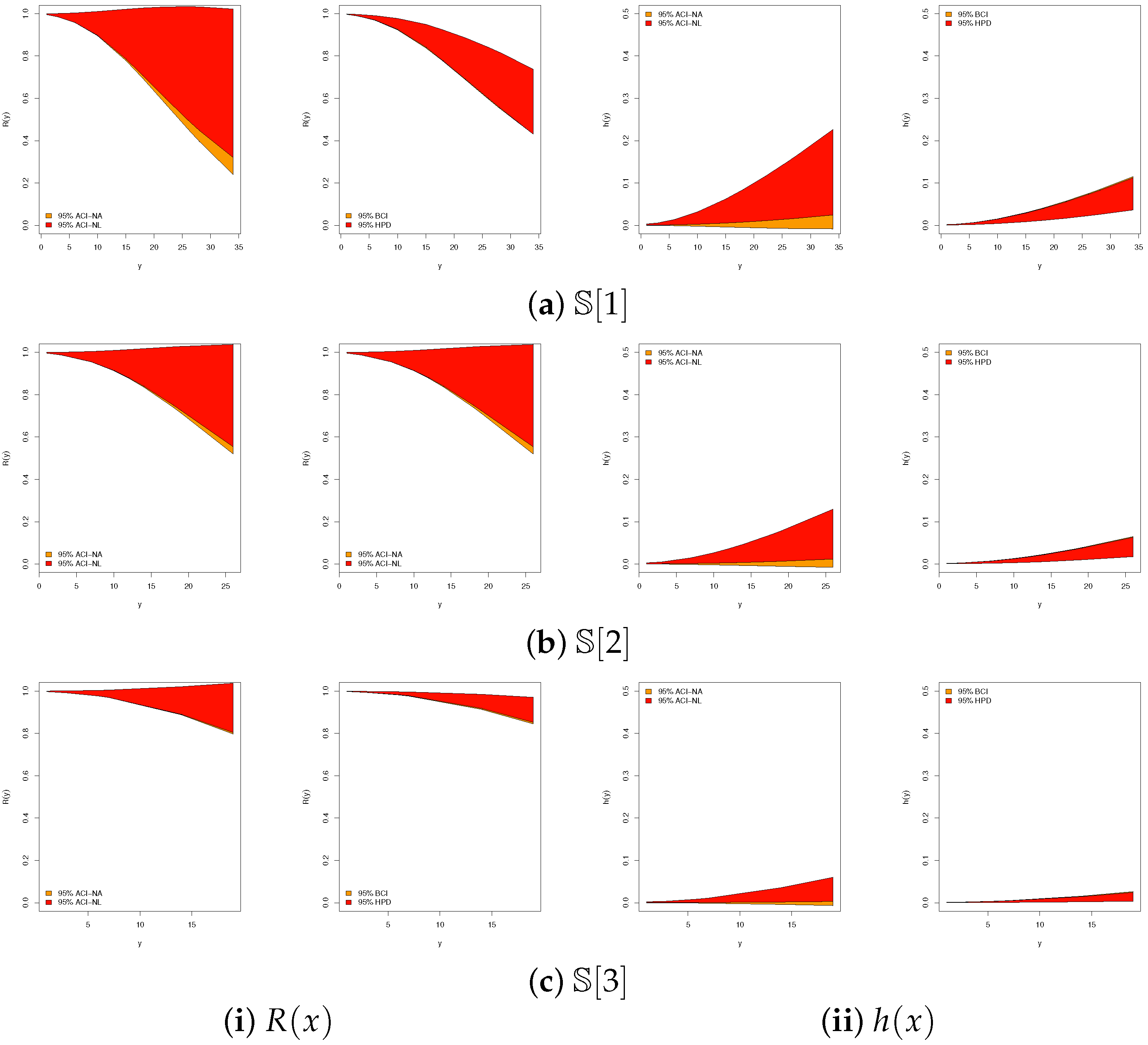
• For all tested values of $\xi$, the Bayesian estimator under Prior-B consistently outperforms alternative approaches, benefiting from the smaller prior variance relative to Prior-A. A parallel advantage is observed when comparing Bayesian intervals (BCI and HPD) to asymptotic ones (ACI-NA and ACI-NL).
• A comparative assessment of the proposed designs of $\mathbf{S}$ in Table 2, for each set of n and r, reveals that:

  -

  Estimates of $\xi$ achieve superior accuracy based on Ci (for $i=1,2$), i.e., right censored sampling;

  -

  Estimates of $h\left(x\right)$ achieve superior accuracy based on Bi (for $i=1,2$), i.e., middle censored sampling;

  -

  Estimates of $R\left(x\right)$ achieve superior accuracy based on Ai (for $i=1,2$), i.e., left censored sampling.

• Regarding interval estimation strategies:

  -

  ACI-NA outperforms ACI-NL for $\xi$ and $h\left(x\right)$, whereas ACI-NL is more suitable for $R\left(x\right)$;

  -

  HPD intervals are uniformly superior to BCIs;

  -

  Overall, Bayesian interval estimators (BCI and HPD) dominate their asymptotic counterparts (ACI-NA and ACI-NL).

• As a conclusion, for reliability practitioners, the ZL lifetime model is most effectively analyzed within a Bayesian framework, leveraging MCMC methods—particularly the Metropolis–Hastings algorithm.

5. Data Analysis

This section is devoted to demonstrating the practical utility of the proposed estimators and validating the effectiveness of the suggested estimation procedures. To this end, we analyze two real-world data sets originating from the fields of medical and physics.

5.1. Clinical Application

Remission time is a critical endpoint in evaluating the effectiveness of treatments for leukemia, as it reflects both the biological response and potential durability of therapeutic interventions. In this study, we focus on remission times, measured in weeks, among leukemia patients who were randomly assigned to receive a specific treatment. Such randomized allocation ensures unbiased comparison and provides a robust framework for assessing treatment efficacy in clinical research. In this application, we shall examine the remission times (measured in weeks) for twenty leukemia patients randomly assigned to a treatment protocol. The corresponding times in ascending order are 1, 3, 3, 6, 7, 7, 10, 12, 14, 15, 18, 19, 22, 26, 28, 29, 34, 40, 48, and 49. The dataset was reported and analyzed by Bakouch et al. [16]. Using the complete leukemia dataset, we assess the adequacy and superiority of the ZL model by comparing its fit with seven alternative models from the literature:

• Xgamma (XG$\left(\xi \right)$) distribution by Sen et al. [17];
• Chris-Jerry (CJ$\left(\xi \right)$) distribution by Onyekwere and Obulezi [18];
• Lindley (L$\left(\xi \right)$) distribution by Johnson et al. [19];
• Exponential (E$\left(\xi \right)$) distribution by Johnson et al. [20];
• Weibull (W$(\alpha ,\xi )$) distribution by Rinne [21];
• Gamma $G(\alpha ,\xi )$ distribution by Johnson et al. [20];
• Nadarajah–Haghighi (NH$(\alpha ,\xi )$) distribution by Nadarajah and Haghighi [22].

In addition to the Kolmogorov–Smirnov ($\mathsf{KS}$) statistic and its associated p-value, we compute several model selection criteria, namely the negative log–likelihood ($\mathsf{NL}$), Akaike information ($\mathsf{AI}$), consistent AI ($\mathsf{CAI}$), Bayesian information ($\mathsf{BI}$), and Hannan–Quinn information ($\mathsf{HQI}$); see

Table 9. Fitting outputs of the ZL and others from leukemia data.

Model	$\mathit{\alpha }$		$\mathit{\xi }$		$\mathsf{NL}$	$\mathsf{AI}$	$\mathsf{CAI}$	$\mathsf{BI}$	$\mathsf{HQI}$	$\mathsf{KS}$
	Est.	SE	Est.	SE						Distance	$\mathit{p}$-Value
ZL	-	-	0.0758	0.0147	78.860	159.720	159.942	160.716	159.914	0.0832	0.9991
XG	-	-	0.1384	0.0187	79.398	160.796	161.019	161.792	160.991	0.1590	0.6928
CJ	-	-	0.1438	0.0192	80.145	162.289	162.511	163.285	162.483	0.1814	0.5262
L	-	-	0.0978	0.0155	78.872	159.745	159.967	160.741	159.939	0.1189	0.9400
E	-	-	0.0512	0.0114	79.460	160.919	161.141	161.915	161.113	0.1143	0.9564
W	1.3081	0.2370	21.155	3.8023	78.884	160.947	161.653	162.939	161.336	0.0903	0.9968
G	1.4634	0.4204	0.0749	0.0256	78.870	161.335	162.041	163.326	161.723	0.0871	0.9981
NH	5.2555	5.3500	0.0064	0.0072	78.878	160.388	161.093	162.379	160.776	0.0847	0.9976

. The MLE and its standard error (SE) are used for fitting all criteria.

To evaluate the suitability of competitive distributions for modeling given lifetime data, the AdequacyModel package (by Marinho et al. [23]) in the R environment is employed. This package provides a comprehensive framework for assessing the goodness-of-fit of parametric models through numerical and graphical techniques. As shown in Table 9, the ZL lifespan distribution consistently provides the most favorable values across all considered criteria compared to its competitors. Thus, based on the leukemia data, the ZL lifetime model demonstrates superior performance relative to the alternative distributions.

To complement the numerical results, Figure 3 presents several graphical diagnostics, including: (i) estimated and fitted RF curves, (ii) probability–probability (PP) plots, (iii) quantile–quantile (QQ) plots, (iv) scaled total time on test (TTT) transform curves, (v) the log-likelihood curve relative to the fitted normal equation, and (vi) a boxplot-overlaid violin plot. From the complete leukemia dataset, Figure 3a–c clearly demonstrate that the ZL model offers an adequate fit, consistent with the goodness-of-fit measures. The TTT plot in Figure 3d suggests an increasing HRF, while Figure 3e confirms both the existence and uniqueness of the MLE $\widehat{\xi }\cong$, making it a reasonable starting value for further estimation. Finally, the distributional features depicted in Figure 3f indicates that the leukemia data distribution is approximately symmetric, with reduced variability and concentration around the median, although a slight right-skewness remains evident.

From the complete leukemia dataset, three synthetic T2I-APC samples are constructed with $r=10$ fixed and different specifications of $\mathsf{S}$ and threshold values ${\tau }_i,i=1,2$, as summarized in

Table 10. Different T2I-APC samples from leukemia dataset.

Sample	$\mathbb{S}$	${\mathit{\tau }}_1\left({\mathit{d}}_1\right)$	${\mathit{\tau }}_2\left({\mathit{d}}_2\right)$	${\mathcal{S}}^{\mathit{🟉}}$	${\mathcal{T}}^{\mathit{🟉}}$	Data
$\mathbb{S}$[1]	$(2\times 5,0\times 5)$	35(10)	40(10)	0	34	1, 3, 6, 10, 15, 18, 22, 26, 28, 34
$\mathbb{S}$[2]	$(0\times 2,2\times 5,0\times 3)$	11(5)	30(10)	4	26	1, 3, 3, 7, 10, 12, 14, 18, 19, 26
$\mathbb{S}$[3]	$(0\times 5,2\times 5)$	15(7)	20(8)	8	20	1, 3, 3, 6, 7, 7, 14, 19

. Since the ZL($\xi$) model is not directly supported by prior information from the leukemia data, an improper gamma prior with hyperparameters $ϵ=\upsilon =0.001$ is adopted for updating $\xi$. The proposed MCMC sampler is initialized using the frequentist point estimates of $\xi$. After discarding the first 10,000 iterations from a total of 50,000, Bayesian point estimates along with credible intervals are obtained for $\xi$, $R\left(x\right)$, and $h\left(x\right)$. For each design $\mathbb{S}\left[i\right]$, $i=1,2,3$,

Table 11. Estimates of $\xi$, $R\left(x\right)$, and $h\left(x\right)$ from leukemia data.

Sample	Par.	MLE		MCMC		ACI-NA			BCI
						ACI-NL			HPD
		Est.	SE	Est.	SE	Low.	Upp.	IL	Low.	Upp.	IL
$\mathbb{S}$[1]	$\xi$	0.0685	0.0188	0.0677	0.0089	0.0317	0.1052	0.0735	0.0506	0.0851	0.0345
						0.0400	0.1171	0.0771	0.0502	0.0846	0.0344
	$R\left(x\right)$	0.9410	0.0012	0.9527	0.0134	0.0041	0.0114	0.0286	0.9239	0.9757	0.9966
						0.0596	0.0806	0.1085	0.9886	0.9691	0.9239
	$h\left(x\right)$	0.1336	0.1446	0.0093	0.0027	0.1692	0.8849	0.9971	0.0046	0.0153	0.0106
						0.0093	0.00	0.9582	0.0043	0.0148	0.0105
$\mathbb{S}$[2]	$\xi$	0.0627	0.0173	0.0618	0.0088	0.0287	0.0966	0.0680	0.0451	0.0794	0.0343
						0.0364	0.1078	0.0714	0.0442	0.0784	0.0341
	$R\left(x\right)$	0.9410	0.0240	0.9611	0.0120	0.8939	0.9881	0.0942	0.9344	0.9813	0.0470
						0.8950	0.9893	0.0943	0.9373	0.9832	0.0459
	$h\left(x\right)$	0.7001	0.0049	0.0076	0.0024	0.6905	0.7097	0.0192	0.0035	0.0131	0.0095
						0.6906	0.7098	0.0192	0.0032	0.0125	0.0093
$\mathbb{S}$[3]	$\xi$	0.0506	0.0160	0.0496	0.0086	0.0193	0.0819	0.0626	0.0334	0.0668	0.0334
						0.0273	0.0939	0.0666	0.0330	0.0663	0.0333
	$R\left(x\right)$	0.9410	0.0173	0.9758	0.0092	0.9071	0.9749	0.0678	0.9548	0.9906	0.0358
						0.9077	0.9755	0.0678	0.9581	0.9926	0.0346
	$h\left(x\right)$	0.7001	0.0035	0.0047	0.0018	0.6933	0.7069	0.0136	0.0017	0.0089	0.0072
						0.6933	0.7070	0.0136	0.0013	0.0083	0.0069

presents the point estimates (with SEs) and corresponding 95% interval estimates (with interval lengths (ILs)) of $\xi$, $R\left(x\right)$, and $h\left(x\right)$ at $x=10$. The findings suggest that the likelihood-based and Bayesian procedures yield comparable estimates for $\xi$, $R\left(x\right)$, and $h\left(x\right)$. Nevertheless, the Bayesian approach generally provides smaller SEs, and its 95% BCI/HPD intervals are narrower than the corresponding 95% ACI-NA/ACI-NL intervals, reflecting improved precision.

To assess the existence and uniqueness of the MLE $\widehat{\xi }$ of $\xi$, Figure 4 displays the log-likelihood profiles along with the associated score functions for all sample settings $\mathbb{S}\left[i\right]$, $i=1,2,3$, over a range of $\xi$ values. Each plot exhibits a single, well-defined maximum, thereby confirming that $\widehat{\xi }$ both exists and is unique. These graphical observations are consistent with the numerical results in Table 11, providing additional support for treating the estimated $\widehat{\xi }$ values as dependable initial points for the subsequent Bayesian analysis.

Convergence of the MCMC samples for $\xi$, $R\left(x\right)$, and $h\left(x\right)$ is assessed through trace plots and posterior density plots shown in Figure 5. The posterior mean and the 95% BCI estimates are highlighted by red solid and dashed lines, respectively. As illustrated in Figure 5, the Markov chains exhibit satisfactory mixing and stabilization for all parameters. The posterior of $\xi$ appears nearly symmetric, whereas $R\left(x\right)$ and $h\left(x\right)$ display negative and positive skewness, respectively. Using the 40,000 post–burn-in samples, several posterior summaries were calculated for $\xi$, $R\left(x\right)$, and $h\left(x\right)$, including the mean, mode, quartiles $\mathcal{Q}\left[i\right],i=1,2,3$, standard deviation (Std.D), and skewness (Sk.); see

Table 12. Statistics of $\xi$, $R\left(x\right)$, and $h\left(x\right)$ from leukemia data.

Sample	Par.	Mean	Mode	$\mathcal{Q}\mathbf{\left[}\mathbf{1}\mathbf{\right]}$	$\mathcal{Q}\mathbf{\left[}\mathbf{2}\mathbf{\right]}$	$\mathcal{Q}\mathbf{\left[}\mathbf{3}\mathbf{\right]}$	SD	Sk.
$\mathbb{S}$[1]	$\xi$	0.06766	0.06053	0.06163	0.06761	0.07361	0.00883	0.05558
	$R\left(x\right)$	0.95266	0.96372	0.94419	0.95366	0.96223	0.01337	−0.45584
	$h\left(x\right)$	0.00936	0.00710	0.00740	0.00915	0.01108	0.00273	0.47232
$\mathbb{S}$[2]	$\xi$	0.06180	0.05835	0.05580	0.06174	0.06767	0.00871	0.06880
	$R\left(x\right)$	0.96107	0.96657	0.95357	0.96209	0.96974	0.01199	−0.52140
	$h\left(x\right)$	0.00765	0.00653	0.00588	0.00743	0.00917	0.00244	0.53929
$\mathbb{S}$[3]	$\xi$	0.04963	0.04569	0.04375	0.04954	0.05536	0.00851	0.08850
	$R\left(x\right)$	0.97584	0.98015	0.97028	0.97685	0.98254	0.00917	−0.67514
	$h\left(x\right)$	0.00466	0.00367	0.00331	0.00445	0.00577	0.00185	0.70214

. These summaries align well with the results reported in Table 11 and the graphical evidence in Figure 5. To further evaluate the convergence behavior of the MCMC chains, ergodic average plots (i.e., cumulative means) were generated for the posterior samples of the parameters $\xi$, $R\left(x\right)$, and $h\left(x\right)$ based on $\mathbb{S}$[1] (as an example); see Figure 6. The trajectories of these running averages flatten after the initial 30,000 burn-in iterations, confirming that the chains have reached stationarity. This visual stabilization, together with the absence of strong autocorrelation patterns, supports the ergodicity of the generated Markov chains and validates the reliability of the Bayesian estimates fitted from the leukemia dataset.

In addition, Figure 7 compares the 95% ACI[NA]/ACI[NL] with the BCI/HPD intervals for $R\left(x\right)$ and $h\left(x\right)$ under the $\mathcal{S}\left[1\right]$ sample from the leukemia data. The BCI/HPD intervals are consistently narrower than their ACI counterparts, reinforcing the superior precision observed in Table 11.

5.2. Physical Application

The River Styx at Jeogla provides a long-term record of annual maximum flood peaks, representing the most extreme discharge events each year. Analysis of these data enables the application of probability models and frequency methods to estimate design floods and recurrence intervals. Consequently, this record serves as a valuable resource for flood risk assessment, hydraulic design, and water resource management in flood-prone regions. In this study, the annual maximum flood peak series for 47 consecutive years from the River Styx (Jeogla) is examined. For computational convenience, the flood peak values in

Table 13. Flooding in the River Styx for 47 years.

0.082	0.130	0.186	0.221	0.224	0.238	0.261	0.267	0.391	0.535
0.580	0.603	0.612	0.626	0.719	0.740	0.799	0.886	0.922	1.050
1.080	1.110	1.170	1.260	1.640	1.770	1.860	1.900	1.940	1.960
2.060	2.200	2.210	2.350	2.550	2.580	2.940	3.000	3.090	3.150
4.050	4.110	4.360	5.130	5.210	5.410	8.780

are scaled by dividing by one hundred, and the transformed dataset is presented. This dataset was previously analyzed by Kuczera and Frank [24] and later reported by Bhatti and Ahmad [25].

Following the same fitting framework described in Section 5.1, we evaluate the adequacy and relative superiority of the ZL model by comparing its performance with seven competing models from the literature, using the complete River Styx dataset. The results in

Table 14. Fitting outputs of the ZL and others from River Styx data.

Model	$\mathit{\alpha }$		$\mathit{\xi }$		$\mathsf{NL}$	$\mathsf{AI}$	$\mathsf{CAI}$	$\mathsf{BI}$	$\mathsf{HQI}$	$\mathsf{KS}$
	Est.	SE	Est.	SE						Distance	$\mathit{p}$-Value
ZL	0.000	0.000	0.685	0.087	76.859	155.718	155.807	157.568	156.414	0.064	0.984
XG	0.000	0.000	1.039	0.105	77.187	156.374	156.463	158.224	157.070	0.070	0.962
CJ	0.000	0.000	1.171	0.112	78.149	158.299	158.387	160.149	158.995	0.113	0.545
L	0.000	0.000	0.819	0.089	77.103	156.207	156.296	158.057	156.903	0.075	0.936
E	0.000	0.000	0.528	0.077	76.978	155.956	156.045	157.807	156.653	0.076	0.932
W	1.090	0.123	1.951	0.275	76.903	157.406	157.679	161.107	158.799	0.065	0.982
G	1.172	0.216	0.620	0.141	76.862	157.242	157.515	160.943	158.635	0.068	0.972
NH	1.214	0.498	0.393	0.247	76.865	157.703	157.976	161.404	159.096	0.066	0.981

show that the ZL model achieves a satisfactory fit, as evidenced by relatively narrow confidence intervals and a high p-value. As illustrated in Figure 8a–c, the ZL model provides an excellent fit to the River Styx data, consistent with the numerical goodness-of-fit measures. Also, Figure 8d confirms the existence and uniqueness of the MLE $\widehat{\xi }\cong 0.6853$, making it a suitable initial value for subsequent computations. Figure 8e suggests an increasing HRF. Finally, Figure 8f reveals that the data are right-skewed with a concentration around lower values, a moderate spread, and one high outlier.

Using the complete River Styx dataset, we generated three artificial T2I-APC samples with a fixed censoring size $r=25$ and different settings of $\mathbb{S}$ and threshold values ${\tau }_i,i=1,2$; see

Table 15. Different T2I-APC samples from River Styx dataset.

Sample	$\mathbb{S}$	${\mathit{\tau }}_1\left({\mathit{d}}_1\right)$	${\mathit{\tau }}_2\left({\mathit{d}}_2\right)$	${\mathcal{S}}^{\mathit{🟉}}$	${\mathcal{T}}^{\mathit{🟉}}$	Data
$\mathbb{S}$[1]	$(2\times 11,0\times 14)$	3.20(25)	3.25(25)	0	3.150	0.082, 0.186, 0.224, 0.238, 0.267, 0.391, 0.535, 0.580, 0.626, 0.719,
						0.799, 0.886, 0.922, 1.110, 1.170, 1.770, 1.860, 1.900, 1.940, 2.350,
						2.550, 2.580, 2.940, 3.000, 3.150
$\mathbb{S}$[2]	$(0\times 7,2\times 11,0\times 7)$	0.95(15)	2.60(25)	6	2.58	0.082, 0.130, 0.186, 0.221, 0.224, 0.238, 0.261, 0.267, 0.535, 0.603,
						0.612, 0.719, 0.740, 0.799, 0.922, 1.050, 1.110, 1.260, 1.770, 1.860,
						1.960, 2.200, 2.210, 2.350, 2.580
$\mathbb{S}$[3]	$(0\times 14,2\times 11)$	1.20(17)	1.95(20)	21	1.95	0.082, 0.130, 0.186, 0.221, 0.224, 0.238, 0.261, 0.267, 0.391, 0.535,
						0.580, 0.603, 0.612, 0.626, 0.719, 0.922, 1.170, 1.260, 1.770, 1.940

. In the absence of prior knowledge about the ZL($\xi$) model, an improper gamma prior with hyperparameters is adopted for updating $\xi$. The MCMC algorithm is initialized with the frequentist point estimates of $\xi$, and a total of $\mathcal{H}=\mathrm{50,000}$ iterations are run, discarding the first ${\mathcal{H}}^{🟉}=\mathrm{10,000}$ as burn-in. Posterior summaries, including Bayesian point estimates and 95% credible intervals for $\xi$, $R\left(x\right)$, and $h\left(x\right)$, are then obtained.

Table 16. Estimates of $\xi$, $R\left(x\right)$, and $h\left(x\right)$ from River Styx data.

Sample	Par.	MLE		MCMC		ACI-NA			BCI
						ACI-NL			HPD
		Est.	SE	Est.	SE	Low.	Upp.	IL	Low.	Upp.	IL
$\mathbb{S}$[1]	$\xi$	0.7793	0.1341	0.7727	0.0998	0.5165	1.0421	0.5255	0.5851	0.9775	0.3924
						0.5562	1.0918	0.5356	0.5748	0.9669	0.3921
	$R\left(x\right)$	0.9410	0.0061	0.9791	0.0045	0.9290	0.9530	0.0239	0.9693	0.9871	0.0178
						0.9291	0.9530	0.0239	0.9699	0.9876	0.0176
	$h\left(x\right)$	0.7001	0.0603	0.2067	0.0447	0.5819	0.8184	0.2365	0.1273	0.3031	0.1759
						0.5913	0.8290	0.2377	0.1229	0.2972	0.1743
$\mathbb{S}$[2]	$\xi$	0.6647	0.1139	0.6602	0.0915	0.4413	0.8880	0.4466	0.4872	0.8462	0.3590
						0.4750	0.9300	0.4551	0.4798	0.8366	0.3568
	$R\left(x\right)$	0.9410	0.0047	0.9840	0.0038	0.9317	0.9503	0.0186	0.9758	0.9907	0.0149
						0.9317	0.9503	0.0186	0.9765	0.9912	0.0146
	$h\left(x\right)$	0.7001	0.0468	0.1585	0.0375	0.6085	0.7918	0.1833	0.0922	0.2389	0.1467
						0.6142	0.7980	0.1838	0.0874	0.2318	0.1444
$\mathbb{S}$[3]	$\xi$	0.4811	0.0922	0.4768	0.0743	0.3005	0.6618	0.3613	0.3377	0.6294	0.2917
						0.3305	0.7004	0.3699	0.3288	0.6180	0.2892
	$R\left(x\right)$	0.9410	0.0031	0.9909	0.0025	0.9349	0.9471	0.0122	0.9854	0.9952	0.0098
						0.9349	0.9471	0.0122	0.9860	0.9956	0.0096
	$h\left(x\right)$	0.7001	0.0307	0.0900	0.0247	0.6399	0.7604	0.1205	0.0475	0.1445	0.0969
						0.6424	0.7630	0.1206	0.0433	0.1378	0.0946

reports the point estimates (with SEs) and interval estimates (with ILs) for each configuration $\mathbb{S}\left[i\right],i=1,2,3$, evaluated at $x=0.1$. The findings reveal close agreement between the likelihood-based and Bayesian methods, though the Bayesian approach achieves smaller standard errors and narrower 95% BCI/HPD intervals compared to the 95% ACI-NA/ACI-NL intervals, highlighting its higher precision.

The existence and uniqueness of the MLE $\widehat{\xi }$ are illustrated in Figure 9, which depicts the log-likelihood functions together with their score counterparts across the three sample configurations $\mathbb{S}\left[i\right],i=1,2,3$. In each case, the curves exhibit a single maximum, confirming both the identifiability of the model and the robustness of the estimation procedure. These visual findings corroborate the numerical results summarized in Table 16, further supporting the choice of $\widehat{\xi }$ as an appropriate initial value in Bayesian computations.

Convergence diagnostics of the MCMC chains for $\xi$, $R\left(x\right)$, and $h\left(x\right)$ are presented in Figure 10, where trace and posterior density plots are supplemented with the posterior mean (red solid line) and the 95% BCI bounds (red dashed lines). The plots confirm stable convergence across all parameters, with an approximately symmetric posterior for $\xi$, and negatively and positively skewed posteriors for $R\left(x\right)$ and $h\left(x\right)$, respectively. Using 40,000 post–burn-in iterations, we computed summary statistics including the posterior mean, mode, quartiles, standard deviation, and skewness (see

Table 17. Statistics for 40,000 MCMC iterations of $\xi$, $R\left(x\right)$, and $h\left(x\right)$ from River Styx data.

Sample	Par.	Mean	Mode	$\mathcal{Q}\left[1\right]$	$\mathcal{Q}\left[2\right]$	$\mathcal{Q}\left[3\right]$	SD	Sk.
$\mathbb{S}$[1]	$\xi$	0.77267	0.76104	0.70429	0.76975	0.83823	0.09959	0.15077
	$R\left(x\right)$	0.97907	0.97975	0.97619	0.97936	0.98225	0.00452	−0.35864
	$h\left(x\right)$	0.20672	0.19992	0.17526	0.20381	0.23516	0.04472	0.36493
$\mathbb{S}$[2]	$\xi$	0.66023	0.64206	0.59791	0.65791	0.72072	0.09143	0.14738
	$R\left(x\right)$	0.98395	0.98486	0.98154	0.98421	0.98662	0.00380	−0.39312
	$h\left(x\right)$	0.15846	0.14953	0.13216	0.15595	0.18229	0.03749	0.39702
$\mathbb{S}$[3]	$\xi$	0.47680	0.46229	0.42641	0.47471	0.52587	0.07418	0.17345
	$R\left(x\right)$	0.99089	0.99151	0.98932	0.99109	0.99265	0.00251	−0.49628
	$h\left(x\right)$	0.09003	0.08397	0.07265	0.08804	0.10555	0.02474	0.49620

), which are fully consistent with the estimates in Table 16. As shown in Figure 11, all ergodic convergence diagnostics based on $\mathbb{S}\left[1\right]$ (as a representative case) indicate that the running averages of $\xi$, $R\left(x\right)$, and $h\left(x\right)$ stabilize rapidly after the burn-in period, confirming the ergodicity and satisfactory convergence of the M-H sampler when the sample information are drawn from the River Styx dataset. In addition,Figure 12 compares the 95% ACI[NA]/ACI[NL] and BCI/HPD intervals for $R\left(x\right)$ and $h\left(x\right)$ based on the $\mathbb{S}\left[1\right]$ River Styx sample, showing that Bayesian intervals are consistently narrower, thereby reinforcing their higher efficiency.

In conclusion, the analyses conducted using samples obtained under the proposed censored dataset, applied to both the leukemia and River Styx datasets, offer a comprehensive evaluation of the ZLindley lifetime model. The findings are consistent with the simulation results and further emphasize the practical utility of the proposed approach in reliability investigations within engineering and physical sciences.

6. Concluding Remarks

This study has advanced the reliability analysis of the ZLindley distribution by embedding it within the improved adaptive progressive Type-II censoring framework. Methodologically, both classical and Bayesian estimation procedures were developed for the model parameters, reliability, and hazard functions. Asymptotic and log-transformed confidence intervals, along with Bayesian credible and highest posterior density intervals, were derived to provide robust inferential tools. The incorporation of MCMC techniques, particularly the Metropolis–Hastings algorithm, ensured accurate Bayesian inference and highlighted the practical benefits of prior information. Through extensive Monte Carlo simulations, the proposed inferential methods were systematically evaluated. The findings confirmed that estimation accuracy improves with larger sample sizes, fewer removals, and higher censoring thresholds. Moreover, Bayesian estimators under informative priors consistently outperformed their frequentist counterparts, and HPD intervals dominated alternative interval estimators in terms of coverage and precision. Importantly, the comparative assessment of censoring schemes demonstrated that left, middle, and right censoring each provide superior accuracy depending on the parameter of interest, offering guidance for practitioners in reliability testing. The practical utility of the proposed methodology was demonstrated through two diverse real-life applications: Leukemia remission times and River Styx flood peaks. In both datasets, the ZLindley distribution outperformed a range of established lifetime models, as confirmed by goodness-of-fit measures, model selection criteria, and graphical diagnostics. These applications validate the model’s flexibility in accommodating both biomedical and environmental reliability data, thereby broadening its applicability in clinical and physical domains. The ZLindley model inherently exhibits a monotonically increasing hazard rate, a behavior commonly associated with ageing or wear-out mechanisms in reliability analysis. This property makes the model suitable for processes where the risk of failure intensifies over time, such as medical survival data under cumulative treatment exposure or environmental stress models like flood levels. However, in systems characterized by early-life failures or mixed failure mechanisms, more flexible distributions such as the exponentiated Weibull, generalized Lindley, or Kumaraswamy–Lindley may provide improved adaptability. Future work could extend the ZLindley framework by introducing an additional shape parameter to capture non-monotonic hazard patterns, thereby broadening its range of applicability. In summary, the contributions of this work are threefold: (i) the integration of the ZLindley distribution with an improved censoring design that ensures efficient and cost-effective testing, (ii) the development of a comprehensive inferential framework combining likelihood-based and Bayesian approaches, and (iii) the demonstration of practical superiority through simulation studies and real data analysis. Collectively, these findings underscore the potential of the ZLindley distribution, under improved adaptive censoring, as a powerful model for modern reliability and survival analysis. Future research may explore its extension to competing risks, accelerated life testing, and regression-based reliability modeling.