Abstract
Tarski’s first-order axiom system for Euclidean geometry is notable for its completeness and decidability. However, the Pythagorean theorem—either in its modern algebraic form or in Euclid’s Elements—cannot be directly expressed in , since neither distance nor area is a primitive notion in the language of . In this paper, we introduce an alternative axiom system in a two-sorted language, which takes a two-place distance function d as the only geometric primitive. We also present a conservative extension of it, which also incorporates a three-place angle function a, both formulated strictly within first-order logic. The system has two distinctive features: it is simple (with a single geometric primitive) and it is quantitative. Numerical distance can be directly expressed in this language. The Axiom of Similarity plays a central role in , effectively killing two birds with one stone: it provides a rigorous foundation for the theory of proportion and similarity, and it implies Euclid’s Parallel Postulate (EPP). The Axiom of Similarity can be viewed as a quantitative formulation of EPP. The Pythagorean theorem and other quantitative results from similarity theory can be directly expressed in the languages of and , motivating the name Quantitative Euclidean Geometry. The traditional analytic geometry can be united under synthetic geometry in . Namely, analytic geometry is not treated as a model of , but rather, its statements can be expressed as first-order formal sentences in the language of . The system is shown to be consistent, complete, and decidable. Finally, we extend the theories to hyperbolic geometry and Euclidean geometry in higher dimensions.
Keywords:
quantitative Euclidean geometry; hyperbolic geometry; distance function; angle function; axiom of similarity; Tarski’s axioms; real closed fields; completeness; decidability MSC:
03B30; 03C35; 51M05; 51M10
Contents
1. Introduction
2. Theory —Quantitative Euclidean Geometry with a Single Geometric Primitive
Notion—Distance Function d
3. Analytic Geometry United under Synthetic Geometry in
4. Theory —A Conservative Extension of with Angle Function a
5. Consistency of and
6. Theory and Tarski’s Are Mutually Interpretable with Parameters
7. Completeness and Decidability of
8. Theory —Quantitative Hyperbolic Geometry
9. Theories and —Quantitative Euclidean Geometry in Higher Dimensions
Appendix A. Axioms of Real Closed Fields (RCF)
Appendix B. Tarski’s Axioms of Plane Euclidean Geometry
Appendix C. SMSG Axioms of Euclidean Geometry
Appendix D. The Convoluted Statement of the Pythagorean Theorem in Tarski’s
1. Introduction
For more than two thousand years, Euclid’s Elements [1] stood as a standard of logical rigor. In the late nineteenth century, however, its shortcomings were exposed, prompting efforts to rebuild Euclidean geometry on firmer foundations. Two milestones were Hilbert’s Grundlagen der Geometrie (1899) [2] and the axiom system developed by Tarski and his students [3,4,5]. Hilbert used natural language, while Tarski introduced a first-order formal system “which can be formulated and established without the help of any set-theoretical devices” [3] (p. 16).
Tarski’s is formulated in a 1-sorted language: the only primitive objects are points. There are two primitive predicate symbols—a 3-place predicate symbol B for betweenness, and a 4-place predicate symbol D for segment congruence—with meaning that lies between and , and meaning segment (as a pair of end points) is congruent to segment . This system has 11 axioms [4,5] (including one axiom schema), which are listed in Appendix B. Tarski established that is complete and decidable.
What part of the content in the Elements is not formalized in ? Notably, contains no notion of area—not even for polygons. In modern mathematics, area is a set function assigning a real number to every measurable set. Even when restricted to polygons, it still requires set-theoretic machinery, which Tarski deliberately avoided in .
The area function of polygons could be discussed in second-order logic, or in first-order logic with two sorts—one sort for points and the other for finite sets of points. The latter approach was discussed by Tarski in his 1959 paper [3], with a sketch of a system as a possible extension of :
Tarski did, however, resolve the decision problem for in his Theorem 5 [3]:“The theory is obtained by supplement the logical base of with a small fragment of set theory. Specifically, we include in the symbolism of new variables assumed to range over arbitrary finite sets of points (or, what in this case amounts essentially to the same, over arbitrary finite sequences of points); we also include a new logical constant, the membership symbol ∈, to denote the membership relation between points and finite point sets. … In consequence the theory of considerably exceeds in means of expression and power. In we can formulate and study various notions which are traditionally discussed in textbooks of elementary geometry but which cannot be expressed in ; e.g., the notions of a polygon with arbitrarily many vertices, and of the circumference and the area of a circle.As regards metamathematical problems which have been discussed and solved for in Theorems 1–4, three of them—the problems of representation, completeness, and finite axiomatizability—are still open when referred to . In particular, we do not know any simple characterization of all models of , nor, do we know whether any two such models are equivalent with respect to all sentences formulated in .”
This follows from the fact that Peano arithmetic (PA) is (relatively) interpretable in .Theorem 5. The theory is undecidable, and so are all of its consistent extensions.
Note that in the same paper [3], Tarski discussed several axiom systems, which he denoted , , , and , but with his primary focus on . Each of these, in his own words, qualifies as a feasible interpretation of “elementary geometry”, and the problem of deciding which is the unique one “seems to be rather hopeless and deprived of broader interest”. For clarity, we retain Tarski’s original symbols when referring to these systems, since terms such as “Tarski’s geometry” or “elementary geometry” are ambiguous. Accordingly, claims like “Euclidean geometry is complete and decidable” or “elementary Euclidean geometry is complete and decidable” are inaccurate, as the systems , , and provide immediate counterexamples.
Having considered the role of area, we now turn to the theory of proportion and similarity, which deals with quantitative relations such as segment lengths. This is the focus of the present paper, which we refer to as Quantitative Euclidean Geometry. In informal treatments of geometry, it is usually taken for granted that every line segment has a length, which is a real number. The Pythagorean theorem provides a good example to illustrate this point. In its modern form, the theorem asserts
for a right triangle, where the bars denote numerical segment lengths. Ancient civilizations also knew this relation. The Egyptians reportedly used a knotted rope to form a 3-4-5 right triangle. In China, it appeared as the gou-gu theorem (or Gougu theorem). Gou and gu refer to the shorter and longer legs of a right triangle respectively, since gu means “thigh” in Classical Chinese. Euclid, however, expressed the theorem differently. In what follows, we examine the possible approaches to the Pythagorean theorem: what has been done, what can be done differently, and what cannot be done within first-order logic and without any appeal to set theory.
- (1)
- The Area Approach by Euclid
The Pythagorean theorem in the Elements is stated as follows [1]:
Proposition I.47 In right-angled triangles the square on the side subtending the right angle is equal to the squares on the sides containing the right angle (Figure 1).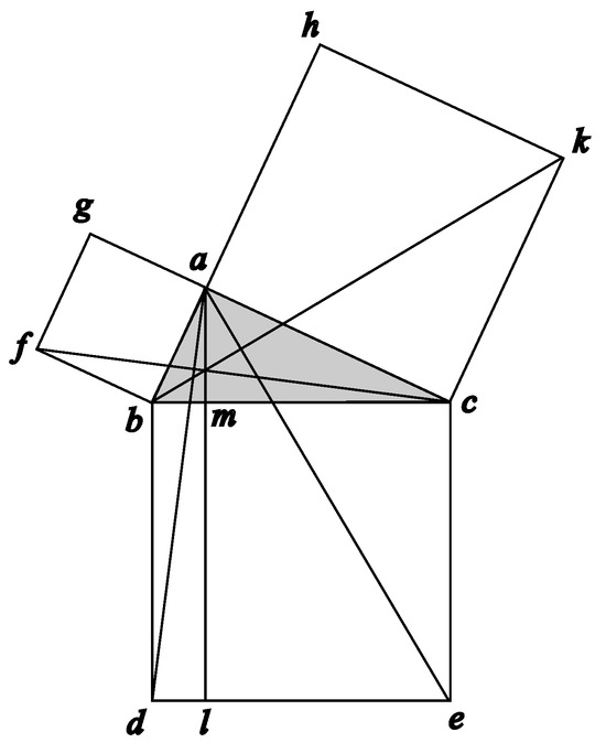 Figure 1. Euclid: the Pythagorean theorem—The notion of area is used to state the theorem.
For Euclid, the square on meant a geometric figure (a rectangle of equal sides), not the numerical product of a length and itself.
What, then, did he mean by saying that one square is equal to two other squares? Euclid did not provide an explicit definition, yet one can infer it from his proof:
Theorem. (Pythagoras-Euclid I.47) In a right triangle, the square on the hypotenuse can be dissected into n triangles, and the union of the two squares on the legs can also be dissected into n triangles with the resulting triangles congruent in pairs.
This formulation cannot be expressed in Tarski’s language , because does not contain a notion of area.
Hilbert developed a theory of area of polygons. His language is informal, and he uses the concept of set freely. Hilbert defines two predicates: equidecomposable and equicomplementable. Consider his definition of “equicomposable”:
In Hilbert’s terms, what Euclid proved in his I.47 is actually: In a right triangle, the square on the hypotenuse is equidecomposable with the union of the two squares on the legs. However, “a finitely number” refers to a natural number, which is not in the language of . The set of natural numbers () is not definable in or in real closed fields (RCF). This helps explain why both and RCF are complete and decidable, while the first-order Peano arithmetic of natural numbers is not.Definition. Two polygons are called equidecomposable if they can be decomposed into a finite number of triangles that are congruent in pairs.
While Hilbert’s theory of area is non-numerical, dealing with equidecomposable and equicomplementable relations only, we may have a theory of area in the numerical form (see Hartshorne [6]). However, an area function that assigns a number to each polygon is a set function, which cannot be part of a first-order language similar to . Consider, for example, a theorem in Hartshorne [6] (p. 206):
A formal first-order language prohibits quantification of functions (such as “there exists a function”), not to mention that the area function is a higher-order function, meaning its domain is a set of sets.Theorem 23.2 In a Hilbert plane with (P), there is an area function , with values in the additive group of the field of segment arithmetic F, that satisfies and is uniquely determined by the following additional condition: For any triangle , whenever we choose one side to be the base and let it have length , and let h be the length of an altitude perpendicular to the base, then .
Thus, the area approach is not viable for us: like Tarski, our aim is to avoid the use of set theory and remain within a first-order framework.
(As a side note, Hartshorne defines a Hilbert plane as one that satisfies Hilbert’s first three groups of axioms, and by (P) he means the axiom of parallels. Thus, this is simply a plane satisfying Hilbert’s first four groups of axioms, but without the axioms of continuity.)
- (2)
- The “Segment Arithmetic” Approach by Hilbert and SST
Here and in what follows, we abbreviate Schwabhäuser, Szmielew, and Tarski [5] as “SST”.
The Pythagorean theorem can also be formulated as the length relationship in Equation (1), and proved using similar triangles. But how do Euclid, Hilbert, and Tarski treat the foundations of proportion and similarity?
The theory of similarity is based on the theorem of Thales, also known as the Fundamental Theorem of Proportion or the Fundamental Theorem of Similarity. This is Proposition VI.2 in the Elements:
Proposition VI.2 If a straight line be drawn parallel to one of the sides of a triangle, it will cut the sides of the triangle proportionally; and, if the sides of the triangle be cut proportionally, the line joining the points of section will be parallel to the remaining side of the triangle (Figure 2).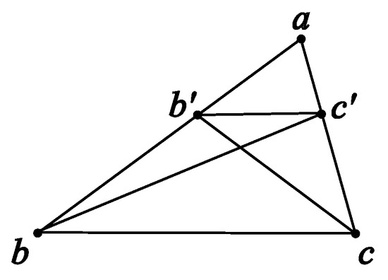 Figure 2. Euclid: Fundamental Theorem of Proportion—The notion of area is not used to state the theorem but used in the proof.
Euclid used the theory of area to prove this Fundamental Theorem of Proportion. He argued that and have “equal-area” because they lie on the same base and are contained between the same parallels and . If we use to denote the area of , this can be written as . Consider and . Their bases and are on the same line, and they have the same altitude. Therefore, . Similarly, if we consider and , we can conclude . Therefore, . Note that we have used modern notation above. Euclid never used the word “area” explicitly.
Here, in this Fundamental Theorem of Proportion, the notion of area is not needed to state the theorem, but Euclid used the theory of area to prove it. Since Tarski’s lacks the notion of area, this proof cannot be carried over to .
If the segments and are commensurable, there exists an elementary proof of this theorem that does not rely on area. However, if and are incommensurable, a limiting process must be invoked; in effect, this limiting method is equivalent to an argument based on area.
Descartes and later Hilbert employed a solution by redefining the multiplication of segments. Consider a right triangle, as shown in Figure 3. They choose the segment as a unit. Suppose and are two points on these orthogonal lines. Draw the line through and , and then draw the line parallel to , intersecting at . The segment is then defined to be the product of and .
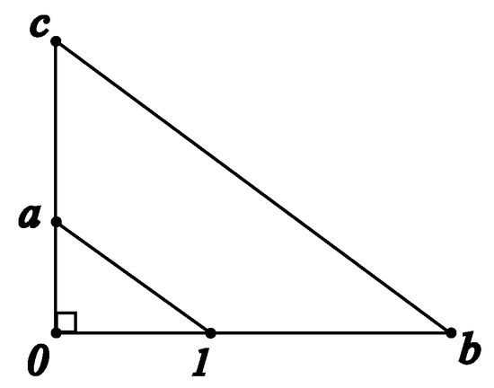
Figure 3.
Descartes and Hilbert: The definition of the product of two segments is a third segment.
As Edwin Hewitt once remarked, “Old theorems never die; they turn into definitions”. Indeed, here the theorem of Thales is turned into the definition of the multiplication of segments. It is important to examine definitions carefully in mathematics. There are cases in mathematical treatments where definitions are made convoluted in order to make the theorems appear simple.
SST [5] carried this further, recasting the segment arithmetic within . They defined addition and multiplication directly on a coordinate line: the “geometric sum” and “geometric product” of two points yield another point on the same line, via projection constructions (see these definitions in Section 6).
The Pythagorean theorem in the form of appears as Theorem 15.8 in SST [5], but this is a highly abbreviated formula with the definitions of geometric product and geometric sum. The complexity of this formula is hidden in the abbreviations (or definitions). When these abbreviations are fully expanded (see Appendix D) using the definition of the geometric product, the theorem becomes a convoluted statement about constructed line segments. Each square is interpreted as a line segment. To Euclid, a segment multiplied by a segment yields a rectangular shape, while to Hilbert and SST, a segment multiplied by a segment yields another segment. So, in SST [5], the meaning of is that two line segments add up to a third segment (see Appendix D).
In summary, we have examined two approaches to the Pythagorean theorem:
(i) Interpreting as (the area of) the shape of a square, as Euclid did. We have concluded that this is not a feasible direction for us to proceed.
(ii) Interpreting as (the equivalence class of) a line segment, constructed using parallel projections, which is indirect and cumbersome.
Besides these two, a third possible approach is the following:
- (3)
- The Numerical Approach by Interpreting as the product of a number and itself
This is the direction we shall pursue in the present paper.
George Birkhoff [7] proposed a system with four postulates, incorporating the notions of numerical measures of lengths and angles. However, it is not a formal system: it freely uses sets, real numbers, and correspondences between sets. For example, he postulates the “ correspondence between the points on a line and the real numbers x” to introduce the distance measure, and the “ correspondence between half-lines and the real numbers a (mod )” to introduce the angle measure.
In 1961, the School Mathematics Study Group (SMSG) developed an axiom system [8] (see Appendix C) intended for American high school geometry courses. Like Birkhoff’s approach, it employs real numbers to measure distances and angles but similarly lacks a formal language framework. While it designates point, line, and plane as undefined terms, this appears to refer only to primitive objects—the system does not explicitly declare undefined predicates or functions. A review of the SMSG axioms reveals that the system implicitly treats the distance function, angle function, area function, and volume function as undefined. Terms such as lie on, lie in, real number, set, contain, as well as correspondence, intersection, and union of sets, are used in the axioms but are not defined. The SMSG axiom list was made large and redundant, and the lack of independence of the axioms was intentional for pedagogical reasons.
The goal of the present paper is to incorporate numerical measures of distances and angles as function symbols into a first-order theory of Euclidean geometry, while avoiding set theory and retaining simplicity. Function symbols are admissible as primitives in first-order logic, since they are special cases of predicates.
We will show that the Axiom of Similarity plays a central role, effectively killing two birds with one stone: it provides the foundation for the theory of proportion and similarity, and it renders Euclid’s Parallel Postulate (EPP) as a theorem. The Axiom of Similarity can be viewed as a quantitative formulation of EPP. The Pythagorean theorem and other quantitative results from similarity theory can then be expressed directly in the first-order languages of and .
2. Theory —Quantitative Euclidean Geometry with a Single Geometric Primitive Notion—Distance Function
- Undefined Primitive Notions
The system is formulated in a first-order formal language
is a 2-sorted language: one sort for points, and the other for numbers. We shall use standard lowercase letters such as for numbers, and boldface lowercase letters such as for points.
The only geometric primitive notion is a 2-place function symbol d, with denoting the distance between two points and , which is a number.
The symbol = is overloaded for convenience: it denotes either the equality of two numbers or the identity of two points, depending on the context.
The symbols + and · are 2-place function symbols for numbers, denoting addition and multiplication. The symbol < is a 2-place predicate symbol for numbers, with denoting that x is less than y.
The symbols 0 and 1 are constant symbols for numbers.
| —The Theory of Plane Quantitative Euclidean Geometry with Distance Function in the Language |
We list the axioms of in the following.
- Axioms RCF1 through RCF17 (for real closed fields, see Appendix A)
RCF1 through RCF17 are the axioms for real closed fields, governing the predicate and function symbols for numbers. This is the first-order formulation of real numbers. As real closed fields are well studied, this is not the focus of the present paper.
Axioms D1 through D7 in the following are geometric axioms, in which all variables range over points, except for x in D4, which ranges over numbers.
- Axiom D1. Axiom of Nonnegativeness
- Axiom D2. Axiom of Identity
- Axiom D3. Axiom of Symmetry
Axioms D1, D2, and D3 are the first three axioms of a metric space. A metric space also includes one more axiom—the triangle inequality. We do not need it as an axiom, as we will prove it in Theorem 8.
- Axiom D4. Axiom of segment extension
- Axiom D5. Axiom of Similarity

Figure 4.
Axiom of similarity.
Figure 4.
Axiom of similarity.

Informal explanation in plain English:
In , suppose cuts and at and respectively. If there is a number k such that and , then
Axiom D5 is expressed in the form of multiplications rather than ratios, because we do not need to use an extra variable k. In addition, an equation of products is more general than an equation of ratios, as we do not need to worry about division by zero.
- Axiom D6. Axiom of Dimension Lower Bound (at least 2)

Figure 5.
The dimension is at least 2.
Figure 5.
The dimension is at least 2.

- Axiom D7. Axiom of Dimension Upper Bound (at most 2)

Figure 6.
The dimension is at most 2.
Figure 6.
The dimension is at most 2.

This concludes the list of axioms for . Note that Tarski’s includes T11—axiom schema of continuity (see Appendix B). We do not require it here, since RCF17 together with D4 implies T11.
- A remark on the dimension axioms:
Axiom D6 can be replaced by a weaker form:
- Axiom D6’. Axiom of Dimension Lower Bound (at least 2)
This asserts that there exist three non-collinear points. When considered in isolation, D6 is strictly stronger than D6’, because D6 implies D6’ but not vice versa. However, in the presence of the rest of the axioms, they are equivalent, since D6’ also implies D6. In general, using an axiom that is too weak may leave certain true statements unprovable, while using one that is too strong may make it no longer independent of other axioms. D6 is independent in the system, because there exists a model of 1-dimensional geometry where D6 fails while all other axioms remain true. When standing alone, the negation of D6 does not imply that the dimension is one. However, the negation of D6 together with the rest of the axioms does imply that the dimension is one. We prefer D6 because it is simpler to state (using primitives only without definitions or abbreviations) and it generalizes more easily to higher dimensions (Section 9). Basically, it is aligned with the affine-independence approach to dimension but stated in metric terms: there exists a nondegenerate 2-dimensional (regular) simplex, but there does not exist a nondegenerate 3-dimensional (regular) simplex. This can be easily generalized to n-dimensional geometry: there exists a nondegenerate n-dimensional (regular) simplex, but there does not exist a nondegenerate ()-dimensional (regular) simplex.
Definition 1.
(Between)
We shall use as the abbreviation for the following:
Note that the betweenness defined here is non-strict, meaning holds if or . To compare, Tarski used non-strict betweenness, while Hilbert used strict betweenness.
Definition 2.
(Collinear)
We shall use as the abbreviation for the following:
Informally, means that the points are collinear.
Definition 3.
(Triangle congruence by SSS)
We shall use as the abbreviation for the following:
Informally, is said to be congruent to if all three pairs of corresponding sides are congruent.
Definition 4.
(Triangle similarity by SSS)
We shall use as the abbreviation for the following:
Informally, is said to be similar to if their three corresponding sides are in proportion. Clearly, triangle congruence is a special case of triangle similarity where .
Traditionally, two triangles are defined to be congruent if all their corresponding sides are congruent and all their corresponding angles are congruent. Two triangles are defined to be similar, if all their corresponding sides are in proportion and all their corresponding angles are congruent. However, it is easy to realize that the conditions on the angles are redundant in these definitions, because the side conditions alone imply that the corresponding angles are congruent—a fact that will be proved as theorems. Therefore, Definitions 3 and 4 differ from the traditional definitions of triangle congruence and triangle similarity found in most textbooks.
Definition 5.
(Angle congruence by docking congruent triangles)
We shall use as the abbreviation for the following:

Figure 7.
Congruence of angles.
Figure 7.
Congruence of angles.

Informally, angle is congruent to angle , if triangle can be “docked” into triangle at the vertex . By “docked”, we mean there exists a triangle such that .
Definition 6.
(Addition of angles)
- Case 1: Addition of non-supplementary angles
If and , we shall use as the abbreviation for the following (this is the case when and are not supplementary):

Figure 8.
Addition of angles—non-supplementary case.
Figure 8.
Addition of angles—non-supplementary case.

- Case 2: Addition of supplementary angles
If ,

Figure 9.
Addition of angles—supplementary case.
Figure 9.
Addition of angles—supplementary case.

Putting the two cases together, we define:
When the angles do not have a common vertex, we may also use . By that, we mean there exist three other angles such that
We can also define the comparison of two angles, or the order of angles.
Definition 7.
(Order of angles)
We shall use the abbreviation for the following:
We also write to mean and
Note that we have defined the sum of two angles and the meaning of one angle is greater than another, but we have not assigned numerical values to angles, because that is not in the language of .
Definition 8.
(Right angle)
We shall use as the abbreviation for the following:

Figure 10.
Right angle.
Figure 10.
Right angle.

Theorem 1.
(Triangle congruence SSS→AAA)
If two triangles are congruent, then their corresponding angles are congruent. Formally,
Proof.
The proof is trivial. The definition of the congruence of two triangles (Definition 3) means the triangles have three sides being congruent respectively. This simply fits the definition of the congruence of each of the three pairs of corresponding angles (Definition 5). □
The reason we include this theorem and the following seemingly simple theorems is that our Definition 3 of triangle congruence is different from most textbooks, and therefore we need to demonstrate how this definition works.
Theorem 2.
(Triangle congruence criterion SAS)
If two triangles have the two sides congruent to two sides respectively, and the angle contained by the two sides congruent, then the two triangles are congruent. Formally,

Figure 11.
Triangle congruence criterion SAS.
Figure 11.
Triangle congruence criterion SAS.

Proof.
By the definition of , there exist on the line and on the line such that .
We first discuss the two possible cases for point .
- Case (1): is between and . In this case we have .
By the definition of , we have .
By the given condition , we must have .
Therefore, .
By Axiom D2, we know . Namely, point coincides with .
- Case (2): is between and . In this case we have .
By the definition of , we have .
By the given condition , we must have .
Therefore, .
By Axiom D2, we know . Namely, point coincides with .
- In the same vein, we can prove that point coincides with .
Therefore, coincides with . Because , we must have . □
Theorem 3.
(Triangle congruence criterion ASA)
If two triangles have two angles congruent to two angles respectively, and the sides adjoining the congruent angles are congruent, then the two triangles are congruent. Formally,

Figure 12.
Triangle congruence criterion ASA.
Figure 12.
Triangle congruence criterion ASA.

Proof. 
By the definition of , there exist points and on line and respectively such that . Because , by a similar argument to that we used in the proof of Theorem 2, we can show that coincides with .
By the definition of , there exist points and on line and respectively such that . By a similar argument, we can show that coincides with .
Now that coincides with , and coincides with , Figure 12 can be simplified as shown below.
Notice that by the definitions of and , we have and . Therefore, . That implies . Since and have the same side , we know must be collinear. Because , must coincide with . Furthermore, because is on both lines and , must coincide with . Namely, all three points coincide. Therefore, . □
Corollary 1.
(Isosceles triangle)
In an isosceles triangle, the base angles are congruent to each other. Formally,

Figure 13.
Isosceles triangle.
Figure 13.
Isosceles triangle.

Proof.
The triangle can be viewed as two triangles in different orientations. The first triangle has three sides , , in this order. The second triangle has three sides , , in this order. The three sides are congruent respectively. Therefore, . By Theorem 1, the corresponding angles are congruent. Namely, . □
Theorem 4.
(Triangle similarity SSS→AAA)
If two triangles are similar, then their corresponding angles are congruent. Formally,

Figure 14.
Corresponding angles of similar triangles are congruent.
Figure 14.
Corresponding angles of similar triangles are congruent.

Proof.
Let . By the given conditions, we have and . By Axiom D5, .
Find the point such that and . Similarly, find the point such that and . By Axiom D5, we have . Therefore, . This implies . Similarly we can prove . □
Theorem 5.
(Triangle similarity criterion AA)
If two triangles have two pairs of corresponding angles congruent, then they are similar. Formally,

Figure 15.
Triangle similarity criterion AA.
Figure 15.
Triangle similarity criterion AA.

Proof.
Let . On line , find the point such that and or . By Axiom D5, is similar to . By Theorem 4, . But it is given that . Therefore, . We say must coincide with , because both and are on the same line . Otherwise it would contradict the fact . Therefore, and , and it implies . □
Theorem 6.
(Interior angle sum of a triangle)
In any triangle , the sum of its interior angles is a straight angle. Formally,

Figure 16.
The interior angle sum of a triangle is a straight angle.
Figure 16.
The interior angle sum of a triangle is a straight angle.

Proof.
The given conditions imply that are the midpoints of , , and respectively. By Axiom D5, . This implies . In the same vein, we can show . Therefore, we have . As a consequence, is congruent to , and is congruent to .
By Axiom D5 again, we have , and . Therefore, we have . As a consequence, is congruent to . Because , , and form a straight angle, the interior angles of the triangle, , , and also “sum up” to a straight angle. □
- It is well known that the interior angle sum theorem is equivalent to Euclid’s Parallel Postulate (EPP), and we will omit the proof of EPP here.
As we can see in the following, using the distance function d, the Pythagorean theorem can be formally and directly stated in the language .
Theorem 7.
(Pythagoras)
where is the abbreviation of .

Figure 17.
The Pythagorean theorem.
Figure 17.
The Pythagorean theorem.

Proof. 
From , drop a perpendicular to and let the foot be , as shown in Figure 17.
First, we want to prove that .
We use proof by contradiction. For the sake of contradiction, suppose that the foot is not between and . Without loss of generality, assume , as shown in the figure below.
Consider the triangle . The interior angles are , , and .
Note that is the sum of and , and is a right angle. is also a right angle.
In the sum of the interior angles of triangle , it includes two right angles ( and ), plus two extra angles ( and ). This contradicts Theorem 6, which asserts the sum of the interior angles of a triangle is equal to a straight angle. Therefore, we must have .
Now consider Figure 17 again.
The triangle is a right triangle. and have two pairs of congruent angles: is congruent to , and is congruent to (both are right angles). By Theorem 5,
Namely,
In the similar vein, we can prove that
Adding Equation (2) to Equation (3), we obtain
□
- The next theorem is the triangle inequality for the distance function.
Theorem 8.
(Triangle inequality)

Figure 18.
Triangle inequality.
Figure 18.
Triangle inequality.

Proof.
From , drop a perpendicular to and let the foot be . The triangle is a right triangle. The point may be between and , or not between and . We discuss three cases:
- Case (1). (Figure 18a)
By Theorem 7, in the right triangle , we have
Because , we have
By Axiom D1, this implies
Similarly, if we consider the right triangle , we obtain
Adding Equation (4) to Equation (5), we obtain
Because , . Therefore,
- Case (2). (Figure 18b)
In the right triangle , similar to Case (1), we have
Because , we have .
By Axiom D1, , we have . Therefore, . This means the single side is at least as long as . When we add a nonnegative length , we have
- Case (3).
The same proof for Case (2) works for this case too, by a symmetry argument. □
Theorem 9.
(Axiom of five segments, see Appendix B)

Figure 19.
Axiom of five segments.
Figure 19.
Axiom of five segments.

Proof. 
Let , , , and .
From , drop a perpendicular to , and let the foot be . From , drop a perpendicular to , and let the foot be (see the figure below).
Let , , and .
- Case (1):
First we want to show, because the two triangles are congruent, , their corresponding altitudes are also congruent, namely .
By the Pythagorean theorem,
Solving these equations, we obtain
In this expression, the altitude h is uniquely determined by the side lengths of . We therefore conclude that the congruent triangle must have the same altitude h.
Now consider the right triangle . By the Pythagorean theorem,
Note that is uniquely determined by , the lengths of the four segments that have their corresponding congruent counterparts in the other configuration with primed points. Therefore, we must have .
- Case (2): If is not between and , the proof is just similar, and we will omit it. The only difference is, the relationship should be replaced by or . □
Theorem 10.
(Axiom of Pasch, inner form, see Appendix B)

Figure 20.
Axiom of Pasch, inner form.
Figure 20.
Axiom of Pasch, inner form.

Proof.
Let , , and .
From , drop a perpendicular to . Let the foot be , and .
- Case (1): is between and .
First, we construct a point in two steps.
- Step 1: On line , find the point between and such that , where
It is easy to see . By Axiom D4, for any number , such a point exists.
- Step 2: From , draw perpendicular to on the side of such that , where
It is easy to see . By Axiom D4, for any number , such a point exists.
We claim that is a point that satisfies and .
Verification of :
By repeated applications of the Pythagorean theorem to the right triangles , , , and , we obtain
It is easy to verify,
Therefore, .
Verification of :
By repeated applications of the Pythagorean theorem to the right triangles , , , and , we obtain
It is easy to verify,
Therefore, .
- Case (2): is not between and .
The proof is similar to Case (1), and we will omit it. □
3. Analytic Geometry United Under Synthetic Geometry in
The mere introduction of a distance function symbol into the language does not by itself render as analytic geometry. Traditionally, synthetic geometry is based on axioms while analytic geometry is based on algebra. In traditional analytic geometry, a point is represented by a pair of real numbers . This is effectively saying that a point is defined to be a pair of real numbers . For two points and , the distance between them is defined to be . In this sense, analytic geometry is treated as a model of synthetic geometry. In contrast, the distance function symbol d in is an undefined primitive notion and is governed by the axioms, rather than being defined. That is why remains synthetic geometry. What makes possible, however, is effectively framing analytic geometry within the formal first-order language of , thereby having synthetic and analytic geometry unified within .
Consider the following example. In traditional analytic geometry, we say has coordinates and has coordinates . Suppose lies on the line passing through distinct points and . If has coordinates , then x and y satisfy the following equation (Figure 21):

Figure 21.
Analytic geometry is united under synthetic geometry in .
Figure 21.
Analytic geometry is united under synthetic geometry in .

The coordinates are related to distances. The precise relation depends on whether they are positive, where
or negative, where
The same applies to all other points as well.
In analytic geometry, one may say informally, “Equation (7) represents the line (or it is the equation of the line) passing through distinct points and ”. We are now ready to express this statement as a formal sentence in :
where is the abbreviation for that all these points being collinear, and the dots indicate analogous conditions for and .
4. Theory —A Conservative Extension of with Angle Function
The language of has a single geometric primitive function d, the distance function, apart from the operations for numbers. We can extend theory further to a theory to include the angle function a, which denotes the numerical measure of an angle.
The language of is
where a is a 3-place function, with being the number to represent the measure of angle formed by points , and , with as the vertex.
The system must satisfy axioms RCF1 through RCF17 (Appendix A), Axioms D1 through D7, plus A1 through A4, which shall be listed in this section.
First, we explain what we mean by being a conservative extension of .
Let be a theory in the language , a theory in the language , and .
is called an extension of if .
is called a conservative extension of if is an extension of , and for each A in , if and only if , meaning the only new theorems in are those that use symbols in that are not in (see Epstein [9]).
In the following, we list the axioms of .
| —The Theory of Plane Quantitative Euclidean Geometry with Distance and Angle Functions in the Language |
- Axioms RCF1 through RCF17
- Axioms D1 through D7
- Axiom A1. Nonnegativeness of angle measure
- Axiom A2. Congruent angles
See Definition 5 in Section 2 for the abbreviation .
Informal explanation in plain English: Congruent angles have equal angle measures and vice versa.
- Axiom A3. Addition of angles

Figure 22.
Addition of angles.
Figure 22.
Addition of angles.

See Definition 6 in Section 2 for the abbreviation .
- Axiom A4. Straight angles
By Axioms A3 and A4, it is easy to see that the maximum value of any angle measure is 180.
Theorem 11.
Informally, this means the angles are undirected. As we can see, there is no need to list this as an axiom. The symmetry of the angle measure is a consequence of the symmetry of distance, .
Proof.
This is straightforward, because by definition, the angles and are congruent. □
Lemma 1.
Proof.
By Axiom A3, if , then . Now consider a special case where , , and . We have
Therefore, . □
Theorem 12.
Informally, if and are on the same “ray”, then the measure of is zero. This shows there is no need to list this as an axiom.
Proof.
Because , by definition, . By Axiom A2 and Lemma 1, . □
Next, we shall prove the theorem of vertical angles in both and separately.
Theorem 13.
(Vertical angles)

Figure 23.
Verticle angles.
Figure 23.
Verticle angles.

Proof.
(Proof in ) Because , and are supplementary angles. Therefore, . Similarly, and are supplementary angles. We have . Therefore, we have . This is the same as . By Axiom A2, we have . □
This is Proposition I.15 in Euclid’s Elements. Euclid’s proof is basically the same as above, except that Euclid did not make the measure of an angle explicit, and he simply cited his Common Notion 3: “If equals be subtracted from equals, the remainders are equal”. Note that we have defined the addition () of two adjacent angles to be a third angle (Definition 6), but there is still a difference between an angle and the measure (as a number) of the angle.
As we have commented, is a conservative extension of . The vocabulary of Theorem 13 does not involve the angle function a. It should be able to be proved in . An alternative proof strictly within the theory is shown in the following.
Proof. 
(Proof within ) By Theorem 12, the points on the same “ray” make the same (congruent) angle. Instead of reasoning with points , we mark points such that , , , and all have the same length. All we have to show is that . To show this, it suffices to show that , because that would guarantee .
First we observe that is an isosceles triangle. Therefore, by Corollary 1, we have .
Consider and . They have a common side . The sides and are congruent. The contained angles and are also congruent. Therefore, by Theorem 2 (SAS). We then have .
Finally we have . Hence, . This is the same as .
□
5. Consistency of and
To show the consistency of , we construct a model that interprets each of the terms in the language
The numbers in are interpreted as the real numbers, as addition and multiplication of real numbers, < the “less than” relation, 0 the number 0, and 1 the number 1.
The real numbers satisfy all the axioms of real closed fields RCF1 through RCF17.
A point is interpreted as a pair of real numbers .
Let and be two points. The distance is interpreted as
Verification of Axioms D1, D2, and D3 is straightforward.
Let . is interpreted as such that
The distance between and is
Verification of Axiom D4:
We discuss two cases.
- Case (1): . For any real number , we can choose
- Case (2): , namely and . It suffices to find such that . Such a point is not unique, but it suffices if we choose
This satisfies and .
- Verification of Axioms D5 through D7 requires just straightforward calculations in analytic geometry, which we shall omit here.
To show the consistency of , first observe that the language is a subset of the language . Recall that
The language has an additional primitive function, the angle function a. The theory is a subtheory of the theory . Therefore, the model we have constructed for can serve as part of a model for . We only need to give an interpretation of the angle function a, and verify Axioms A1 through A4.
Let , , , , and , as shown in Figure 24.

Figure 24.
Interpretation of the angle measure.
Figure 24.
Interpretation of the angle measure.

We first define
The angle measure of is interpreted as
Verification of Axioms A1 through A4 requires just straightforward analytic geometry calculations, which are omitted here.
6. Theory and Tarski’s Are Mutually Interpretable with Parameters
6.1. There Is a Syntactical Translation from to
Tarski’s is parameter-free interpretable in . This interpretation is faithful. In addition, we can make a stronger assertion than a faithful interpretation: there is a syntactical translation from to (see definitions of interpretation and syntactical translation in Enderton [10]).
The syntactical translation scheme is as follows:
Any variable in is translated to a point variable in .
Tarski’s primitive predicates in are translated to as follows:
- (1)
- is translated to:
- (2)
- is translated to:
Tarski’s axioms T1 through T11 for are listed in Appendix B.
T5 (Axiom of five segments) is proved as Theorem 9, T7 (Axiom of Pasch) as Theorem 10 in Section 2. Other axioms are straightforward to verify in , using the above syntactical translation, and Axioms D1 through D7 plus RCF1 through RCF17.
6.2. Theory Is Interpretable (with Parameters) into
To interpret in , we devise a mapping from to .
Any point variable in remains a point variable in .
We also need to find a way to interpret the number variables of in , because has only point variables but no number variables. This can be done with the help of the segment arithmetic with respect to an arbitrarily selected frame of three points , , and which are non-collinear.
We first select any three non-collinear points , , and .
Our sub-universe in is all the points on the line of , which are used to interpret the numbers of RCF. The constant 0 is mapped to , and the constant 1 is mapped to . We will call the line the number line.
We will use the following convention in notation: a hat is used to denote a point on the number line. For example, the symbol automatically implies that (see Definition 2).
Figure 25 shows SST’s definition [5] that point is the geometric sum of points and . We will omit the formal sentence, but just describe it informally:
Join and with a line;
Draw , intersecting at (‖ denotes parallel);
Draw ;
Draw , intersecting at ;
Draw , intersecting at .
We then define as the geometric sum of and . In symbols, we write

Figure 25.
The definition that point is the geometric sum of points and .
Figure 25.
The definition that point is the geometric sum of points and .

Figure 26 shows SST’s definition [5] that point is the geometric product of points and . Informally:
Join and with a line;
Join and with a line;
Draw , intersecting at ;
Draw , intersecting at .
We then define as the geometric product of and . In symbols, we write

Figure 26.
The definition that point is the geometric product of points and .
Figure 26.
The definition that point is the geometric product of points and .

It should be noted that RCF is a subtheory of . We first describe how to interpret sentences in RCF into , namely those sentences in that involve number variables only.
Each number variable x is mapped to a point variable for a point on the number line in . For example, the wff (well-formed formula) in RCF (also in ) will be interpreted as in . The wff in RCF (also in ) will be interpreted as in .
In the language , there are only three atomic predicate symbols:
- (1)
- = as a 2–place predicate denoting that two points are identical.
- (2)
- = as a 2-place predicate denoting that two numbers are equal.
- (3)
- < as a 2-place predicate denoting that one number is less than the other.
First, consider the case where = is a predicate for points, for example, . This is already a valid wff in and it can be kept as is.
Next, consider the case where = is a predicate for numbers. We have discussed a special case when both sides of the equation involve number constants and variables only. In general, we also need to consider the function symbol . The following is an example of a wff in :
where are point variables, and are number variables.
Note that 2 is the abbreviation of , and 3 is the abbreviation of .
Therefore, 1 is interpreted as , 2 is interpreted as , and 3 is interpreted as .
The entire wff can be interpreted as
In the language of , the Pythagorean theorem (Theorem 7) asserts
This can be interpreted in as
This interpretation scheme works the same for the predicate < in .
- The interpreted formula can often be simplified for special cases. The following are two types of wffs that are most frequently encountered in :
(1) can be interpreted as in .
(2) can be interpreted as
in .
7. Completeness and Decidability of
In the previous section, we have established that is mutually interpretable (with parameters) to and the interpretation if faithful. Because it has been shown that is complete and decidable, is also complete and decidable.
8. Theory —Quantitative Hyperbolic Geometry
We briefly provide a sketch of a theory of quantitative hyperbolic geometry. Its language is the same as with two sorts.
We only need to replace Axiom D5 of with Axiom D5-h, and retain the rest of the axioms in , as listed below. We shall not go into the details in this direction.
| : The Theory of Plane Quantitative Hyperbolic Geometry with Distance and Angle Functions in the language of |
- Axioms RCF1 through RCF17
- Axioms D1 through D4
- Axiom D5-h. (AAA→SSS) Given two triangles, if all three pairs of angles are equal, then their sides are congruent.
- Axioms D6, D7
- Axioms A1 through A4
9. Theories and —Quantitative Euclidean Geometry in Higher Dimensions
Both systems and can be generalized to and for n-dimensional Euclidean geometry (). We only need to replace the two dimension axioms D6 and D7 with D6-n and D7-n, as described below.
- Axiom D6-n. Dimension lower bound (at least n)
- Axiom D7-n. Dimension upper bound (at most n)
We will not discuss further in this direction.
Funding
This research received no external funding.
Data Availability Statement
No new data were created or analyzed in this study. Data sharing is not applicable to this article.
Acknowledgments
The author thanks Michael Beeson, Julien Narboux, and Pierre Boutry for valuable discussions, and the anonymous reviewers for their careful reading of the paper and their insightful comments.
Conflicts of Interest
The author declares no conflicts of interest.
Appendix A. Axioms of Real Closed Fields (RCF) [9]
- The Theory of Real Closed Fields in the Language of
Note that 0 and 1 are constant symbols, denoting the identity of addition and the identity of multiplication respectively. The constant 0 is definable by the formula , and the constant 1 is definable by . We can have an equivalent theory in the language of after replacing the constants 0 and 1 with the above definitions, but we choose to include these constants in the language for convenience.
- RCF1.
- RCF2.
- RCF3.
- RCF4.
- RCF5.
- RCF6.
- RCF7.
- RCF8.
- RCF9.
- RCF10.
- RCF11.
- RCF12.
- RCF13.
- RCF14.
- RCF15.
- RCF16.
- RCF17.
where is any wff in which x is free, is any wff in which y is free, and neither y nor z appear in , and neither x nor z appear in . ( is the abbreviation for .)
Appendix B. Tarski’s Axioms of Plane Euclidean Geometry [4,5]
The following are Tarski’s axioms for as listed in [4,5]. Tarski included thirteen axioms, A1 through A13, in his 1959 paper [3], but A2 and A3 were proved as theorems later. The remaining axioms in [3] are the same as listed below, only in different order.
- The Theory in the language of
denotes that point is between and .
denotes that point pair is congruent to point pair .
- T1. Symmetry of congruence
- T2. Transitivity of congruence
- T3. Identity of congruence
- T4. Segment extension
- T5. Five segments

Figure A1.
Five segments.
Figure A1.
Five segments.

- T6. Identity of betweenness
- T7. Pasch (inner form)

Figure A2.
Inner Pasch.
Figure A2.
Inner Pasch.

- T8. Dimension lower bound
- T9. Dimension upper bound

Figure A3.
The dimension is at most 2.
Figure A3.
The dimension is at most 2.

- T10. Euclid

Figure A4.
Euclid.
Figure A4.
Euclid.

- T11. Axiom schema of continuity (Dedekind cut)

Figure A5.
Continuity.
Figure A5.
Continuity.

Appendix C. SMGS Axioms of Euclidean Geometry [8]
- Undefined terms: point, line, plane.
The officially listed undefined terms are: point, line, plane. However, there are also undefined terms (objects, predicates, and functions) that are used in the axioms but are not explicitly listed, such as: distance measure, angle measure, area, volume, lie on, lie in, real number, set, contain, correspondence, intersection, and union.
- Postulate 1. (Line Uniqueness) Given any two different points, there is exactly one line which contains them.
- Postulate 2. (Distance Postulate) To every pair of different points there corresponds a unique positive number.
- Postulate 3. (Ruler Postulate) The points of a line can be placed in a correspondence with the real numbers in such a way that
(1) To every point of the line there corresponds exactly one real number, (2) To every real number there corresponds exactly one point of the line, and (3) The distance between two points is the absolute value of the difference of the corresponding numbers. - Postulate 4. (Ruler Placement Postulate) Given two points P and Q of a line, the coordinate system can be chosen in such a way that the coordinate of P is zero and the coordinate of Q is positive.
- Postulate 5. (Existence of Points)
a. Every plane contains at least three non-collinear points. b. Space contains at least four non-coplanar points. - Postulate 6. (Points on a Line Lie in a Plane) If two points lie in a plane, then the line containing these points lies in the same plane.
- Postulate 7. (Plane Uniqueness) Any three points lie in at least one plane, and any three non-collinear points lie in exactly one plane.
- Postulate 8. (Plane Intersection) If two different planes intersect, then their intersection is a line.
- Postulate 9. (Plane Separation Postulate) Given a line and a plane containing it, the points of the plane that do not lie on the line form two sets such that:
(1) each of the sets is convex and (2) if P is in one set and Q is in the other then segment intersects the line. - Postulate 10. (Space Separation Postulate) The points of space that do not lie in a given plane form two sets such that
(1) each of the sets is convex and (2) if P is in one set and Q is in the other then segment intersects the plane. - Postulate 11. (Angle Measurement Postulate) To every angle there corresponds a real number between 0 and 180.
- Postulate 12. (Angle Construction Postulate) Let be a ray on the edge of the half-plane H. For every r between 0 and 180 there is exactly one ray , with P in H, such that .
- Postulate 13. (Angle Addition Postulate) If D is a point in the interior of , then .
- Postulate 14. (Supplement Postulate) If two angles form a linear pair, then they are supplementary.
- Postulate 15. (SAS Postulate) Given a correspondence between two triangles (or between a triangle and itself). If two sides and the included angle of the first triangle are congruent to the corresponding parts of the second triangle, then the correspondence is a congruence.
- Postulate 16. (Parallel Postulate) Through a given external point there is at most one line parallel to a given line.
- Postulate 17. (Area of Polygonal Region) To every polygonal region there corresponds a unique positive number.
- Postulate 18. (Area of Congruent Triangles) If two triangles are congruent, then the triangular regions have the same area.
- Postulate 19. (Summation of Areas of Regions) Suppose that the region R is the union of two regions and . Suppose that and intersect at most in a finite number of segments and points. Then the area of R is the sum of the areas of and .
- Postulate 20. (Area of a Rectangle) The area of a rectangle is the product of the length of its base and the length of its altitude.
- Postulate 21. (Volume of Rectangular Parallelpiped) The volume of a rectangular parallelpiped is equal to the product of the altitude and the area of the base.
- Postulate 22. (Cavalieri’s Principle) Given two solids and a plane. If for every plane which intersects the solids and is parallel to the given plane the two intersections have equal areas, then the two solids have the same volume.
Appendix D. The Convoluted Statement of the Pythagorean Theorem in Tarski’s
In Section 1, we noted that SST [5] presents the Pythagorean theorem (Theorem 15.8) in the form
At first glance, this may seem to be the familiar modern algebraic form of the Pythagorean theorem; however, it is not, because the language of cannot express the length of a segment as a number. The terms , , and are all abbreviations. The term means the geometric product of and , denoted by . Precisely, Equation (A1) should be expanded as
where and denote geometric sum and geometric product respectively. These are defined by parallel projections using the segment arithmetic (see the definitions in Section 6).
In what follows, we present the complete sentence corresponding to Equation (A1) after these abbreviations are fully expanded.
Let be a triangle with being a right angle (Figure A6).
- (1)
- Choose an arbitrary point on . We will take as the unit length.
On line , locate a point such that . Join and with a line.
Through , draw a line parallel to , and let it intersect at .
By the definition of geometric product, .
- (2)
- Join and with a line.
On line , locate a point such that .
Through , draw a line parallel to , and let it intersect at .
By definition, .
- (3)
- On , find a point such that . Hence, also has unit length.
On line , locate a point such that .
Join and with a line.
Through , draw a line parallel to , and let it intersect at .
By definition, .
Finally, Equation (A1) can be expressed as . To prove this theorem, it suffices to show is congruent to .

Figure A6.
The convoluted statement of the Pythagorean theorem using segment arithmetic: Segment is equal to the sum of and .
Figure A6.
The convoluted statement of the Pythagorean theorem using segment arithmetic: Segment is equal to the sum of and .

The preceding description is informal. When the Pythagorean theorem in the form of Equation (A1) is expressed in the formal language of , it becomes:
where
Equation (A2) is a convoluted formula. In this form, the Pythagorean theorem is not the same theorem as Proposition I.47 in Euclid’s Elements, and neither theorem implies the other without establishing a nontrivial connection between area and segment arithmetic (see Hartshorne [6] (p. 179)).
The notion of geometric product employed here is a variant of Hilbert’s definition, using a skewed frame rather than an orthogonal frame. Although it is not exactly the definition given by SST [5], it is equivalent to it. Had we adopted their definition verbatim (see Figure 26 in Section 6), the formal statement of the Pythagorean theorem would have been even longer.
In contrast, the language of permits the Pythagorean theorem to be expressed in the simple form
This provides part of the motivation for the present paper.
References
- Heath, T. The Thirteen Books of Euclid’s Elements, 2nd ed.; Dover: New York, 1956. [Google Scholar]
- Hilbert, D. Foundations of Geometry, 2nd ed.; Open Court: La Salle, 1971. [Google Scholar]
- Tarski, A. What is elementary geometry? In The Axiomatic Method with Special Reference to Geometry and Physics, Proceedings of the International Symposium, University of California, Berkeley, CA, USA, 26 December 1957–4 January 1958; Studies in Logic and the Foundations of Mathematics; Henkin, L., Suppes, P., Tarski, A., Eds.; North-Holland: Amsterdam, 1959; pp. 16–29. [Google Scholar]
- Tarski, A.; Givant, S. Tarski’s system of geometry. Bull. Symb. Log. 1999, 5, 175–214. [Google Scholar] [CrossRef]
- Schwabhäuser, W.; Szmielew, W.; Tarski, A. Metamathematische Methoden in der Geometrie; Springer: Berlin, 1983; reprint by Ishi Press: New York, 2011. [Google Scholar]
- Hartshorne, R. Geometry: Euclid and Beyond; Springer: New York, 2000. [Google Scholar]
- Birkhoff, G.D. A set of postulates for plane geometry based on scale and protractor. Ann. Math. 1932, 33, 239–345. [Google Scholar] [CrossRef]
- School Mathematics Study Group. Geometry: Student’s Text; Yale University Press: New Haven, 1961. [Google Scholar]
- Epstein, R. Classical Mathematical Logic; Princeton University Press: Princeton, 2006. [Google Scholar]
- Enderton, H.B. A Mathematical Introduction to Logic, 2nd ed.; Harcourt/Academic Press: San Diego, 2001. [Google Scholar]


Disclaimer/Publisher’s Note: The statements, opinions and data contained in all publications are solely those of the individual author(s) and contributor(s) and not of MDPI and/or the editor(s). MDPI and/or the editor(s) disclaim responsibility for any injury to people or property resulting from any ideas, methods, instructions or products referred to in the content. |
© 2025 by the author. Licensee MDPI, Basel, Switzerland. This article is an open access article distributed under the terms and conditions of the Creative Commons Attribution (CC BY) license (https://creativecommons.org/licenses/by/4.0/).