Abstract
Accurate and reliable credit risk classification is fundamental to the stability of financial systems and the efficient allocation of capital. However, with the rapid expansion of customer information in both volume and complexity, traditional rule-based or purely statistical approaches have become increasingly inadequate. Motivated by these challenges, this study introduces a domain-constrained stacking ensemble framework that systematically integrates business knowledge with advanced machine learning techniques. First, domain heuristics are embedded at multiple stages of the pipeline: threshold-based outlier removal improves data quality, target variable redefinition ensures consistency with industry practice, and feature discretization with monotonicity verification enhances interpretability. Then, each variable is transformed through Weight-of-Evidence (WOE) encoding and evaluated via Information Value (IV), which enables robust feature selection and effective dimensionality reduction. Next, on this transformed feature space, we train logistic regression (LR), random forest (RF), extreme gradient boosting (XGBoost), and a two-layer stacking ensemble. Finally, the ensemble aggregates cross-validated out-of-fold predictions from LR, RF and XGBoost as meta-features, which are fused by a meta-level logistic regression, thereby capturing both linear and nonlinear relationships while mitigating overfitting. Experimental results across two credit datasets demonstrate that the proposed framework achieves superior predictive performance compared with single models, highlighting its potential as a practical solution for credit risk assessment in real-world financial applications.
MSC:
68T07
1. Introduction
With the advent of the big data era, financial technology (FinTech) has rapidly transformed the credit industry, accelerating the shift from traditional offline lending to online platforms and expanding access to diverse forms of consumer credit [1]. At the same time, the proliferation of digital credit reporting systems has significantly reduced the marginal cost of acquiring customer information, providing financial institutions with unprecedented opportunities to evaluate borrower risk profiles. Accurate and reliable credit evaluation has, therefore, become not only a cornerstone of financial stability but also a key driver of efficient capital allocation in the digital economy.
In recent decades, logistic regression (LR) has been widely regarded as a fundamental approach in credit scoring, valued for its ease of use, transparency, and compliance with regulatory standards [2]. It has been successfully applied across diverse financial settings, from cross-domain transfer learning in credit risk prediction [3] to large-scale risk control systems in Western financial institutions. Meanwhile, the rise of machine learning has introduced alternative classifiers such as support vector machines (SVM), random forests (RF), and neural networks, which demonstrate strong predictive performance by capturing nonlinear and nonparametric relationships [4,5,6]. More recent advances, including gradient boosting algorithms such as XGBoost and deep attention-based architectures like TabNet [7], further highlight the potential of advanced algorithms in handling structured credit data. However, purely data-driven models are often criticized for their lack of transparency and potential misalignment with regulatory standards [8]. In addition, the predictive capacity of individual models remains inherently constrained, which motivates the exploration of ensemble methods.
Ensemble learning, including boosting, bagging, and stacking, has thus attracted increasing attention in credit risk prediction. Boosting algorithms such as XGBoost [9], LightGBM [10], and CatBoost [11] have achieved remarkable success on structured tabular data, while random forest ensembles provide robustness to noisy inputs and multicollinearity [12]. Stacking, in particular, offers a principled way to combine heterogeneous base learners through a layered architecture, allowing models to exploit complementary strengths and mitigate individual weaknesses [13,14]. These properties make stacking highly suitable for credit default prediction, where both linear relationships and complex nonlinear interactions must be effectively captured. Nevertheless, existing ensemble-based studies often focus primarily on model performance while overlooking the integration of domain knowledge and business rules, which are crucial for interpretability, regulatory compliance, and practical deployment in financial institutions. This gap creates new opportunities for research at the intersection of domain expertise and ensemble modeling.
Motivated by these considerations, this study proposes a domain-constrained stacking ensemble framework for credit default prediction. The framework systematically embeds domain heuristics into the modeling pipeline, including threshold-based outlier detection to enhance data quality, target variable redefinition to align with industry practice, and monotonicity-constrained binning to ensure stability of predictor-response relationships. Following this, features are transformed using Weight-of-Evidence (WOE) encoding and evaluated via Information Value (IV), enabling effective dimensionality reduction while retaining interpretability. On this structured feature space, three predictive models—logistic regression, random forest, and XGBoost—are employed as base learners, while their cross-validated out-of-fold predictions are combined through a meta-level logistic regression in a two-layer stacking ensemble. This design balances the strengths of linear and nonlinear modeling while reducing overfitting risk, yielding a robust and interpretable framework that bridges domain constraints with advanced ensemble learning techniques.
The contributions of this paper can be summarized as follows:
- We propose an ensemble-based modeling approach that combines multiple complementary classifiers within a unified stacking architecture to enhance credit default prediction.
- The framework integrates domain-informed constraints with a structured feature engineering pipeline, incorporating monotonicity-constrained binning, Weight-of-Evidence (WOE) transformation, and Information Value (IV)-based feature selection, which aligns with both statistical rigor and industry conventions.
- Extensive experiments conducted on two benchmark credit datasets demonstrate that the proposed approach consistently outperforms individual classifiers in terms of predictive accuracy and robustness.
The remainder of this paper is organized as follows. Section 2 reviews related literature on credit risk modeling and ensemble methods. Section 3 introduces the proposed framework, including domain-informed feature engineering and predictive modeling strategies. Section 4 presents the experimental design and performance evaluation. Finally, Section 5 concludes the paper and outlines future research directions.
2. Related Work
In this section, we analyze the extant literature along two dimensions, namely traditional credit scoring approaches, and machine learning and ensemble methods.
2.1. Traditional Credit Scoring Approaches
Credit default prediction has traditionally relied on demographic and socioeconomic characteristics, such as age, income, marital status, education, family size, and residential stability [15,16,17]. Such characteristics determine both the inclination and the capability of borrowers to fulfill repayment obligations, forming the foundation of early credit scoring practices. For instance, higher education attainment has been shown to improve repayment performance, while income and loan size remain consistent determinants of default probability [18].
From a methodological perspective, early models were dominated by statistical techniques such as linear discriminant analysis, Bayesian classifiers, and logistic regression [19,20]. Among these methods, logistic regression has long been recognized as the prevailing benchmark in credit scoring, primarily for its methodological simplicity, transparency, and regulatory endorsement [2]. However, such models rely on assumptions of linearity and independence among predictors, limiting their ability to capture nonlinear dependencies and interaction effects in borrower behavior [21]. While widely used as benchmarks, these models face increasing challenges in handling the complexity and scale of modern financial data.
2.2. Machine Learning and Ensemble Methods
With the advent of machine learning, a novel class of models has emerged that alleviates the restrictive assumptions of conventional statistical methods. Among them, support vector machines (SVMs) are extensively used in default risk modeling, owing to their robustness and versatility in classification [22]. Decision tree ensembles, such as random forests, are valued for their resilience to noise and multicollinearity, and for handling imbalanced datasets effectively [12,23]. Gradient boosting algorithms, including XGBoost and related variants, further enhance predictive performance on structured credit data [9,24]. More recently, deep neural networks (DNNs) have been employed to capture complex nonlinear relationships, showing superior performance in bankruptcy and credit risk prediction compared to logistic regression and other traditional models [25,26]. Furthermore, behavioral signals extracted from unstructured sources, such as loan application texts, have opened new avenues for enhancing credit risk assessment [27].
Despite these advances, single-model approaches remain constrained by structural limitations. Ensemble learning has, therefore, emerged as a promising strategy to improve generalization and robustness [14]. Bagging methods such as random forests and boosting methods such as XGBoost, LightGBM, and CatBoost have been extensively applied in financial risk prediction tasks [10,11]. Stacking, in particular, provides a principled way of integrating heterogeneous classifiers within a multi-layer architecture [13]. Recent studies confirm that stacking ensembles can outperform single classifiers in credit scoring, bankruptcy prediction, and financial inclusion tasks [28,29]. Beyond these applications, recent methodological advancements have further expanded the scope of stacking. Ersoy et al. proposed a stacking regression framework for macroeconomic time-series forecasting, showing that alternative loss functions, such as absolute deviation, can enhance robustness under regime shifts [30]. Similarly, Liu et al. developed a dynamic integrated stacked regression model with adaptive weighting for multi-source agricultural data, highlighting the benefits of dynamically adjusting ensemble composition [31]. In a complementary direction, Chen et al. analyzed error reduction from stacked regressions under an empirical risk minimization framework, establishing the theoretical advantage of regularized weight learning in stacked ensembles [32].
Beyond predictive accuracy, growing attention has been directed toward model explainability and domain-informed design in credit scoring. Post-hoc interpretation techniques, such as SHAP and LIME, have been widely adopted to visualize local feature contributions and enhance regulatory transparency [33,34]. In parallel, domain-grounded approaches have re-emerged that rely on statistical indicators such as Weight-of-Evidence and Information Value, which remain widely recognized in financial institutions for their interpretability, monotonicity control, and regulatory acceptance [2,4]. In addition, hybrid frameworks that embed explainability mechanisms into machine learning pipelines have also gained momentum [35,36,37].
A growing body of research has emphasized that, despite substantial progress in model explainability and predictive performance, domain or expert knowledge remains insufficiently integrated into modern credit risk modeling. Guan et al. [38] propose a hybrid knowledge-acquisition framework for responsible credit assessment, emphasizing that expert rules are rarely embedded in current machine learning pipelines. Likewise, Valdrighi et al. [39] review recent ML-based credit scoring practices and report that, while predictive accuracy has steadily improved, the incorporation of expert input and regulatory constraints remains limited. These observations reveal a persistent gap between data-driven modeling and domain-informed credit risk practices. To bridge this gap, the present study introduces a domain-constrained stacking framework that systematically embeds business-informed feature engineering—such as rule-based data cleaning, monotonic binning, and stability-oriented transformations—into the modeling pipeline and integrates them with ensemble learning strategies. By combining linear and nonlinear classifiers within a unified stacking architecture, the framework aligns with established credit risk principles while enhancing predictive accuracy and interpretability.
3. Methodology
3.1. Problem Description
We formulate credit default prediction as a binary classification task. For each individual i, let denote the feature vector with attributes, and let the label be , where represents a reliable customer (no severe default) and denotes a risky customer (severe default). The learning objective is to construct a mapping function, , that minimizes the expected prediction error as the following:
where denotes the hypothesis space and is a classification loss. The detailed description of feature variables is provided in Table 1. Among them, refers to the data label, and – are the ten-dimensional features used.

Table 1.
Variable description and data types.
3.2. Overall Framework
The proposed framework integrated data preparation, feature transformation, and predictive modeling into a unified pipeline, as illustrated in Figure 1. The process began with exploratory data analysis (EDA) to examine data distributions, structures, and potential anomalies. Structured domain constraints were then applied for pre-processing, including outlier removal and missing value handling, ensuring data consistency. Next, feature binning and WOE transformation were performed, accompanied by the IV analysis to assess discriminatory power and filter weak predictors. This yielded a compact and structured feature space aligned with credit risk practices.
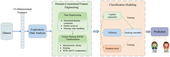
Figure 1.
The framework of credit default prediction model.
On top of this feature set, three base models were trained: a logistic regression model to capture the linearized WOE effects and preserve interpretability, a random forest model to represent complex nonlinear interactions through bagging, and an XGBoost model to enhance gradient-based learning and fine-grained feature discrimination. These base learners were further integrated using a two-layer stacking ensemble, which leverages the complementary strengths of linear and nonlinear models. This design effectively bridged domain-informed feature engineering with data-driven learning, yielding a coherent and high-performance framework for credit default prediction.
3.3. Exploratory Data Analysis
The Exploratory Data Analysis (EDA) constitutes a crucial initial step in the modeling pipeline, providing an overall understanding of the dataset prior to feature engineering and model construction [40]. In this work, EDA was conducted on all eleven features, including the target label distribution, to obtain a holistic view of both predictor behavior and class balance. This allowed not only characterizing each attribute but also early detecting of class imbalance, outliers, and anomalous patterns.
The analysis began with a preliminary cleaning of the raw dataset, followed by a systematic inspection of each feature. For each attribute, its type, range, and distribution were assessed through descriptive statistics and visual methods. This process helped flag violations of domain logic—such as infeasible values, extreme tails, or inconsistent ranges. Continuous variables were further examined for distributional shape and boundary violations, while categorical or count features were checked for rare categories or highly skewed frequencies. Missing data was evaluated in terms of both frequency and plausible mechanisms, informing decisions on imputation, or deletion strategies.
Insights derived from EDA played two foundational roles: First, they motivated the incorporation of domain-informed constraints in subsequent pre-processing: setting plausible thresholds, aligning the target variable with industry conventions, and selecting variables for discretizations. Second, they served as the empirical basis for the feature transformation stage—particularly binning, WOE encoding and IV screening [41]. In this way, EDA formed the bridge between raw data and modeling-ready features, ensuring the processing pipeline was grounded in both empirical evidence and domain logic.
3.4. Feature Binning and WOE/IV Transformation
To facilitate subsequent model construction and ensure consistency with credit scoring practices, all features were transformed through a binning and WOE encoding procedure. This process served two main purposes as follows: (i) It converted raw attributes into a log-odds scale that was directly compatible with logistic regression. (ii) It provided an objective measure of variable predictive strength through IV [41,42].
For continuous attributes, an automatic binning procedure was applied. Starting from an initial number of intervals, the variable was partitioned into equal-frequency bins and the monotonicity between bin means and default rates was checked using Spearman correlation. The number of bins was iteratively adjusted until monotonicity was satisfied. The final output consisted of bin boundaries, WOE values, and the IV score. The procedure is summarized in Algorithm 1. Methods enforcing monotonic binning were studied in the literature to improve scorecard stability and interpretability [43].
For discrete or long-tailed variables, bin boundaries were defined using domain knowledge and prior exploratory analysis. This custom binning procedure discretized the feature according to pre-defined cut-points, computed WOE values for each bin, and aggregated the IV score. The steps are outlined in Algorithm 2. Similar approaches blending domain rules with binning were advocated in scorecard development [44].
Given a feature partitioned into bins i, let and denote the proportions of positive and negative samples in bin i, respectively. The WOE and IV are computed as the following:
Figure 2 provides an overview of the complete feature engineering workflow, covering pre-processing, binning strategies, WOE/IV computation, and the replacement of raw features with WOE-encoded representations.
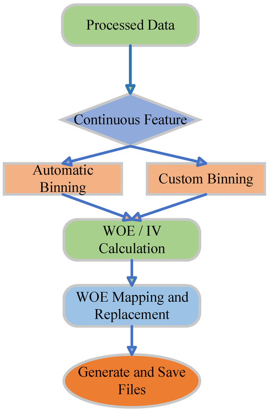
Figure 2.
Feature engineering workflow for binning and WOE/IV transformation, including automatic and custom binning, WOE encoding, and output generation.
Finally, original feature values are replaced with their corresponding WOE codes in both training and testing sets. This transformation not only aligns with industry conventions, but also helps reduce the influence of outliers and enforces a linear log-odds mapping to the default target, thereby enhancing modeling stability and interpretability [45,46].
| Algorithm 1 Monotonic automatic binning (mono_bin) |
|
| Algorithm 2 Custom binning algorithm (self_bin) |
|
3.5. Data-Driven Modeling
After domain-informed pre-processing and feature transformation, the modeling stage focused on capturing complementary patterns of default risk through three representative classifiers: logistic regression, random forest, and XGBoost. Each model contributed distinct learning mechanisms, and their integration within a stacking ensemble was designed to enhance predictive performance and robustness.
Logistic Regression (LR). Logistic regression models the conditional probability of default as a logistic function of the features as the following:
which leads to a probability form as the following:
Parameter estimation was performed by maximizing the log-likelihood:
with
LR offers high computational efficiency and strong compatibility with WOE-encoded features, as the linearized representation aligns with its modeling assumptions.
Random Forest (RF). Random forest is a bagging-based ensemble that constructs multiple decision trees from bootstrap resamples of the dataset, introducing feature-level randomness at each split. Its predictive mechanism can be expressed as the following:
where denotes the m-th tree’s prediction and M is the total number of trees. RF effectively modeled nonlinear dependencies and interaction effects while maintaining robustness to outliers and multicollinearity.
Extreme Gradient Boosting (XGBoost). XGBoost is a boosting-based algorithm that builds additive decision trees sequentially to minimize a regularized loss function:
where denotes the tree added at the t-th iteration and is a regularization term controlling tree complexity. The gradient-based optimization enables XGBoost to capture subtle feature interactions and improve convergence speed, making it well-suited for structured financial data.
Stacking Ensemble. Stacking (stacked generalization) integrates these heterogeneous base learners within a hierarchical architecture. In the first layer, optimized LR, RF, and XGBoost models serve as base classifiers. Using stratified K-fold cross-validation, out-of-fold predictions from each base learner are generated, forming three meta-features that collectively encode linear, bagging-based, and boosting-based perspectives of default risk. These meta-features are then fed into a second-layer logistic regression model (the meta-learner), which learns the optimal combination of base outputs. This layered integration allows the ensemble to balance interpretability, diversity, and nonlinear expressiveness, achieving improved generalization compared to any single model.
In summary, the data-driven component of the framework leverages complementary classifiers—logistic regression, random forest, and XGBoost—whose integration through stacking ensures that both linear regularities and complex nonlinear patterns of credit default risk are effectively captured.
4. Experimental Results and Analysis
4.1. Dataset Description
In this study, two publicly available benchmark datasets were employed for credit default prediction: the Give Me Some Credit (GMSC) dataset and the German Credit Data. The GMSC dataset (https://www.kaggle.com/c/GiveMeSomeCredit (accessed on 25 September 2025)) is a large-scale benchmark widely adopted in both academic and industrial research on credit risk modeling. Originally released through the 2011 Kaggle competition on credit scoring (competition period: 19 September 2011–16 December 2011), it aims to predict whether a borrower will experience serious delinquency (90 days or more past due) within the next two years. The dataset contains 150,000 training instances and 101,503 testing instances, as defined by the official competition split. Among the training samples, 10,026 correspond to defaults and 139,974 to non-defaults, yielding an imbalanced default rate of approximately 6.7%. Each record is described by ten predictive attributes (–) and one binary target label (), as summarized in Table 1. To ensure consistency with industry standards, the target variable SeriousDlqin2yrs was inverted (1 − SeriousDlqin2yrs) so that non-defaulters are represented by 1 and defaulters by 0. This transformation aligns with the convention used in WOE and IV computations, where the ratio of “good” to “bad” clients is defined with “good” corresponding to 1. For model evaluation, the datasets were randomly partitioned into training and testing subsets with a ratio of 7:30.
In addition to the GMSC dataset, the German Credit Data dataset was also incorporated to validate the generalization capability of the proposed framework across heterogeneous credit domains. This dataset served as a complementary benchmark characterized by a smaller scale and richer categorical representation, providing an interpretable perspective on model behavior. A comprehensive description of its variable composition, data pre-processing, and the exploratory data analysis (EDA) is provided in Appendix A.
4.2. Evaluation Metrics
To comprehensively evaluate both the baseline classifiers (logistic regression, random forest, and XGBoost) and the proposed ensemble framework (Stacking), a set of six well-established performance metrics was employed: accuracy, recall, F1-Score, Area Under the Receiver Operating Characteristic Curve (AUC-ROC), G-Mean, and Kolmogorov–Smirnov (KS) statistic. These metrics collectively capture both overall correctness and the discriminative capability of the models under class-imbalanced conditions.
- (1)
- Multi-dimensional Evaluation Metrics
Accuracy, recall, and the F1-Score were adopted as core scalar indicators of classification performance. Accuracy measures the overall proportion of correctly classified instances. Recall quantifies the model’s ability to identify actual defaulters, and the F1-Score provides a balanced summary by combining precision and recall through their harmonic mean. Their definitions are as follows:
- (2)
- Curve-based Evaluation Metrics
To further assess discriminative power, the AUC–ROC was employed. The ROC curve illustrates the trade-off between the True Positive Rate (TPR) and the False Positive Rate (FPR) across varying classification thresholds as the following:
The AUC–ROC aggregates this relationship into a single scalar value:
where higher values indicate stronger separation between defaulters and non-defaulters.
- (3)
- Geometric Mean (G-Mean)
The G-Mean metric evaluates the balance between sensitivity (recall) and specificity (true negative rate). It is particularly useful in imbalanced datasets, ensuring that the model performs well for both positive and negative classes as follows:
where . A higher G-Mean indicates that the classifier maintains consistent accuracy across both majority and minority classes.
- (4)
- KS Statistic
The Kolmogorov–Smirnov (KS) statistic measures the maximum distance between the cumulative distributions of predicted scores for defaulters and non-defaulters as follows:
where and denote the cumulative distribution functions of scores for non-defaulters and defaulters, respectively. A larger KS value reflects better discriminatory ability, with values above 0.3 generally regarded as acceptable in practical credit scoring applications.
Overall, these six complementary metrics provide a balanced and interpretable assessment of model performance, enabling a robust comparison between single learners and the proposed stacking ensemble.
4.3. Exploratory Data Analysis and Pre-Processing Results
This section presents the exploratory data analysis (EDA) conducted specifically on the GMSC dataset, along with the corresponding pre-processing strategies applied to improve data quality and ensure robust model training. The GMSC dataset comprises eleven predictive features (–, see Table 1) in addition to the binary target label. The EDA results reveal several important characteristics, including pronounced class imbalance, the existence of outliers, and heterogeneous patterns of missing values across features. These empirical observations directly guided the design of the subsequent pre-processing procedures and modeling pipeline, ensuring that the derived features are both statistically sound and operationally meaningful for credit default prediction.
Target distribution. As shown in Figure 3a, the dataset exhibits a pronounced class imbalance, where non-defaulters substantially outnumber defaulters. To alleviate this skew, the Synthetic Minority Oversampling Technique (SMOTE) was applied to the training set during pre-processing, generating synthetic minority samples to achieve a more balanced class distribution while preventing data leakage.
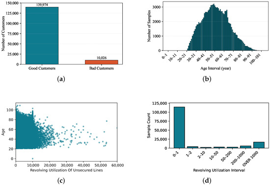
Figure 3.
Feature distributions of –: (a) class distribution of defaulted and non-defaulted; (b) age feature distribution; (c) joint distribution of revolving credit utilization and age; and (d) distribution of debt ratio categories.
Age. The distribution of Age (Figure 3b) approximates a normal shape but contains clear anomalies. Implausible records include borrowers with age as well as ages above 96 years, with the maximum observed at 109. Such outliers are considered noise and are removed. Table 2 further shows the default rates across age intervals: individuals aged 18–40 exhibit the highest default rate (10.08%), which declines monotonically with increasing age.
Table 2.
Default rate by age interval.
Credit utilization (Revolving Utilization Of Unsecured Lines). As a percentage, this variable should theoretically lie in , with values exceeding one indicating overdrawn accounts. To facilitate visualization, the horizontal axis in Figure 3c was scaled by multiplying by 10,000. A substantial fraction of data points fall above one, which may stem from missing denominators or reporting errors. We stratified the anomalous region into , , , , and . Table 3 reports default rates across these bins, with the peak (57.14%) observed in , suggesting potential error thresholds. Consequently, values exceeding 20 are treated as outliers.
Table 3.
Default rate by utilization interval.
Debt ratio. Empirical evidence indicates that values of debt ratio above two are highly anomalous. As shown in Figure 3d and Table 4, the data distribution and corresponding default rates indicate that default risk peaks in the interval but stabilizes thereafter. Accordingly, values greater than two are considered outliers.
Table 4.
Default rates across different debt ratio intervals.
Real estate loans (Number Real Estate Loans Or Lines). The distribution (Figure 4a) shows that values are clear anomalies. Hence, an upper cutoff of 50 was applied.
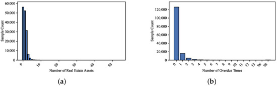
Figure 4.
Feature distributions of –: (a) distribution of real estate loan counts and (b) sample distribution of delinquency frequency.
Dependents (Number Of Dependents). This variable contains 3924 missing values (2.62%). Considering the relatively small proportion of missing entries, both deletion and simple imputation were initially feasible options. To determine the most appropriate strategy, we conducted a comparative experiment evaluating the effects of direct deletion versus median imputation under the same modeling pipeline.
Monthly income (Monthly Income). This feature exhibits 29,731 missing values (19.82%). Since the proportion approaches 20%, simple deletion would severely distort the dataset. Therefore, to preserve the predictive information contained in this variable, a random forest regression–based imputation method was employed to estimate the missing values using the remaining observed features.
Delinquency counts (Number of times 90 days late,Number of time 30–59 days past due not worse,Number of time 60–89 days past due not worse). As illustrated in Figure 4b and Table 5 and Table 6, extreme values exceeding 90 were implausible and treated as anomalies. These adjustments ensure that the processed dataset was both statistically reliable and suitable for subsequent model training.
Table 5.
Distribution of overdue times (Feature ).
Table 6.
Distribution of overdue times (Feature ).
As detailed in the preceding EDA analysis, all thresholds for outlier detection and discretization were determined empirically based on the observed feature distributions and default-rate patterns. Following these observations, a systematic pre-processing pipeline was developed to enhance data quality and ensure stable model training.
To determine the most reliable missing-value strategy, a controlled experiment was conducted comparing two alternatives: (i) deletion of samples containing missing entries, and (ii) median imputation, both implemented under an identical pipeline comprising binning, WOE transformation, and subsequent model construction. Predictive performance was assessed using ROC–AUC and complementary metrics. As shown in Table 7, the deletion-based approach consistently outperformed median imputation, indicating that removing limited missing samples yields more stable downstream performance. Consequently, this study adopts the deletion method for variables with few missing entries, while applying a random forest based imputation for variables with high missingness.
Table 7.
Comparison of AUC–ROC performance under different missing-value treatments.
Following the exploratory analysis, additional data-cleaning procedures were applied to remove inconsistencies and implausible records. An unused index column (Unnamed: 0) was deleted, and duplicate rows were dropped. Rule-based filtering was used to exclude unrealistic values, including samples with non-positive ages and extreme delinquency counts (number of time 30–59 days past due not worse, number of time 60–89 days past due not worse, or number of times 90 days late ) and excessively large values of number real estate loans or lines (≥50). The variable Monthly Income was imputed via a random forest regressor trained on remaining numerical features, while records missing number of dependents were removed. These pre-processing steps ensured that the dataset was internally consistent and suitable for subsequent modeling.
4.4. Feature Selection
To further enhance the interpretability of the proposed framework, a quantitative feature relevance analysis was conducted using the IV metric. IV provides a well-established measure of the predictive power of each variable with respect to the binary default outcome, offering a transparent means to evaluate the contribution of domain features within credit scoring tasks. In addition to interpretability, the IV metric also serves as an effective criterion for feature selection, enabling the identification and filtering of weak predictors prior to model training. In this study, the IV threshold was set to 0.20 for the GMSC dataset and 0.10 for the German Credit dataset.
For the GMSC dataset, the IV ranking revealed that revolving utilization of unsecured lines (0.9819), number of times 90 days late (0.8486), number of time 30–59 days past due not worse (0.7309), and number of time 60–89 days past due not worse (0.5658) were the most influential predictors, indicating that delinquency-related behaviors and credit utilization play a decisive role in default discrimination. In contrast, features such as debt ratio (0.0186) and number of dependents (0.0345) exhibited limited information value, suggesting a weaker association with credit risk. For the German Credit dataset, the analysis identified account status (0.6660), history credit (0.2932), saving account (0.1960), and credit purpose (0.1692) as the most informative features, reflecting their strong connection to repayment behavior and financial stability. Conversely, variables like dependents (0.0000) and Address (0.0036) contributed minimally to the prediction process.
The resulting IV distributions were visualized using horizontal bar plots (Figure 5), which clearly illustrate the ranking and relative importance of all features across datasets. This analysis not only complements the exploratory data analysis but also provides a practical and interpretable foundation for feature selection, offering insights into the feature-level determinants that drive model performance in credit default prediction.
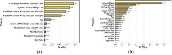
Figure 5.
Comparison of model performance under different missing-value treatments: (a) Information Value (IV) ranking of features on the GMSC dataset; and (b) Information Value (IV) ranking of features on the German Credit dataset.
4.5. Model Performance Evaluation
Experiment I: Baseline Performance Comparison. In this experiment, testing was conducted separately on two benchmark datasets, and the results are presented in Table 8 and Table 9. All reported values represent the mean ± 95% confidence interval obtained over five independent runs under identical experimental settings. The best results in each column are highlighted in bold.
Table 8.
Performance comparison of different models on the GMSC dataset.
Table 9.
Performance comparison of different models on the German Credit dataset. Bold values indicate the best performance within each column.
The experimental findings indicate that the proposed Stacking Ensemble consistently achieves the highest overall performance across both datasets. For the GMSC dataset, the ensemble model attains the best scores in AUC–ROC (0.8725), F1-Score (0.9761), and KS (0.587), demonstrating enhanced discriminative capability in distinguishing defaulters from non-defaulters. The random forest exhibits the highest recall (0.9880), highlighting its sensitivity to minority (default) samples, while logistic regression provides stable AUC and precision values. The XGBoost model also demonstrates strong predictive capability, confirming the effectiveness of boosting-based methods for structured financial data. Its competitive performance complements the strengths of logistic regression and random forest, jointly contributing to the ensemble’s stable and balanced predictive behavior. A similar trend is observed on the German Credit dataset, where the proposed approach achieves superior results in AUC–ROC (0.8951), accuracy (0.892), and KS (0.6012). The relatively narrow confidence intervals across all models indicate that the observed performance differences are statistically consistent rather than caused by random variation.
Overall, the Stacking Ensemble effectively integrates the complementary strengths of base learners—including linear (logistic regression), bagging-based (random forest), and boosting-based (XGBoost) algorithms—providing stable and reliable predictive performance across two credit default datasets.
The fitted meta-learner coefficients give an overview of how important the different models are within the ensemble. To further examine their relative contributions, we analyzed the learned coefficients across the two benchmark datasets, as summarized in Table 10. For the GMSC dataset, the logistic regression base learner receives a negative weight (), whereas both random forest () and XGBoost () obtain strong positive coefficients. This suggests that the meta-level model counterbalances the linear learner’s overconfident predictions by emphasizing the nonlinear corrections provided by the tree-based models. In contrast, for the German Credit dataset, all base learners exhibit positive coefficients (, , and for logistic regression, random forest, and XGBoost, respectively), with random forest again showing the largest contribution. This indicates that after domain-constrained pre-processing—such as WOE transformation and monotonic binning—the data become more linearly separable, allowing all models to contribute synergistically to the final prediction. Overall, the results confirm that while stacking ensembles consistently benefit from nonlinear learners, the relative importance and sign of each base model remain data-dependent. The meta-learner adaptively allocates weights according to the intrinsic structure and separability of each dataset, achieving a well-balanced trade-off between interpretability and predictive performance.
Table 10.
Meta-learner coefficients of the stacking ensemble across datasets.
Experiment II: Model Uncertainty Estimation. Traditional classifiers output a probability score for each class, yet such scores often fail to express the model’s confidence in its predictions. This limitation becomes particularly critical in financial risk management. For example, a predicted probability of 0.6 may carry different implications depending on whether it is consistently estimated or varies widely across models. Uncertainty estimation thus complements conventional performance metrics by quantifying prediction reliability and stability.
Gal and Ghahramani [47] introduced dropout-based Bayesian approximations for uncertainty estimation, leveraging predictive variance or entropy as proxies. Inspired by their framework, this study applied uncertainty estimation in a structured-data setting to enhance model interpretability and robustness.
- (1)
- Random Forest Ensembles
For random forest models, uncertainty was quantified by the dispersion of predicted probabilities across individual trees. A high degree of consensus among trees implies low uncertainty, whereas divergent outputs indicate high uncertainty.
Let M denote the number of independently trained random forest sub-models. For a test sample x, the m-th sub-model outputs the probability of belonging to the positive class. The mean prediction and standard deviation are given by the following equations:
where reflects the consensus probability, while quantifies the model’s predictive uncertainty. A higher implies greater disagreement among base learners and lower prediction confidence. The distribution of values across the dataset is presented in Figure 6.
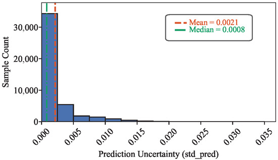
Figure 6.
Uncertainty distribution estimated from the random forest ensemble.
- (2)
- XGBoost Model
Gradient-boosting models such as XGBoost iteratively reduce residual errors through sequential additive learning. However, they typically output point estimates without explicit uncertainty quantification. To assess prediction reliability, this study adopted a bootstrapped ensemble inference strategy for XGBoost. Multiple models were trained on resampled subsets of the training data, and the variability among their predicted probabilities represented epistemic uncertainty.
Let T denote the number of bootstrap models. For each sample x, the t-th model yields , and the aggregated mean and dispersion are as the following:
where denotes the average predicted probability, while captures model disagreement. Figure 7 illustrates the resulting uncertainty distribution, where a sharp concentration near zero indicates that most XGBoost predictions are highly confident. Compared with random forest, XGBoost exhibits a slightly narrower uncertainty spread, reflecting smoother probabilistic calibration and stronger regularization effects.
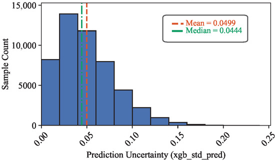
Figure 7.
Uncertainty distribution estimated from the XGBoost model.
- (3)
- Logistic Regression and Stacking Mode
Unlike ensemble methods, single models such as logistic regression cannot exploit variance across sub-models. Instead, their uncertainty is quantified using entropy of the predicted probability :
The Stacking ensemble in this study adopted logistic regression as the meta-learner. Its uncertainty estimation follows the same entropy-based approach:
where denotes the meta-learner’s predicted probability. Figure 8a,b illustrate the distribution of uncertainty scores for logistic regression and Stacking, respectively.
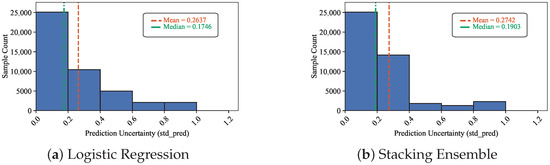
Figure 8.
Uncertainty distributions of logistic regression and Stacking models.
Uncertainty histograms reveal that lower median and mean entropy values correspond to higher model confidence. Moreover, a peak density near zero indicates that most predictions are highly certain. Combining classification metrics (Table 8 and Table 9) with uncertainty analyses (Figure 6, Figure 7 and Figure 8), the Stacking ensemble demonstrated superior overall performance. It not only achieved the highest AUC, KS, and F1-score but also maintained stable and reliable uncertainty distributions, outperforming both random forest and logistic regression. Therefore, the Stacking model was selected as the final classifier for subsequent applications.
Experiment III: Model Training Efficiency. To assess the computational efficiency of the proposed domain-constrained stacking framework, the training time of all compared models was measured on both datasets. The results, summarized in Table 11, reveal that simple models such as logistic regression and XGBoost exhibit very fast convergence due to their lightweight parameter structures and gradient-based optimization. Random forest requires slightly longer training time owing to iterative tree construction.
Table 11.
Training time comparison across different models on the GMSC and German Credit datasets.
The Stacking Ensemble represents the total training time of the proposed two-layer pipeline, including the base learners (LR, RF, and XGBoost) as well as the meta-level logistic regression. On the larger GMSC dataset, the entire pipeline completes within 2.55 s, whereas on the smaller German Credit dataset, the total time is approximately 1.23 s, reflecting the smaller data scale and lower model complexity. Overall, the results indicate that the proposed framework maintains high computational efficiency and demonstrates promising applicability in real-world credit risk modeling scenarios.
Experiment IV: IV Threshold Sensitivity Analysis. To further evaluate the robustness of the domain-constrained feature selection strategy, a sensitivity analysis was conducted by varying the IV threshold used for variable retention. Since IV quantifies the predictive power of individual features under monotonic Weight-of-Evidence encoding, different thresholds directly affect the number of selected variables and the final model performance. The stacking ensemble was re-trained under multiple IV cutoffs to investigate the stability of classification metrics.
Figure 9 illustrates the effect of IV thresholds on the GMSC dataset. As the IV threshold increases from 0.1 to 0.9, the number of retained variables gradually decreases from five to one. The model achieves its best overall discrimination performance around the threshold of 0.2, with both AUC and KS reaching peak values (0.8725 and 0.5879, respectively). Beyond this point, the removal of moderately informative variables leads to a decline in predictive capability, indicating that overly aggressive filtering may reduce model diversity.
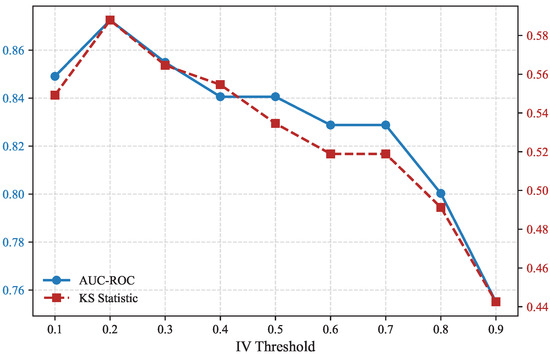
Figure 9.
IV threshold sensitivity analysis on the GMSC dataset.
A similar experiment was performed on the German Credit dataset (Figure 10). The results exhibit a consistent pattern, where moderate thresholds (0.09–0.11) yield the most balanced trade-off between AUC (0.8951) and KS (0.6012). When the threshold is too low, irrelevant features introduce noise; when it is too high, useful but weak predictors are discarded. These findings validate that the IV-based filtering mechanism is robust and that the model performance remains stable within a reasonable threshold range.
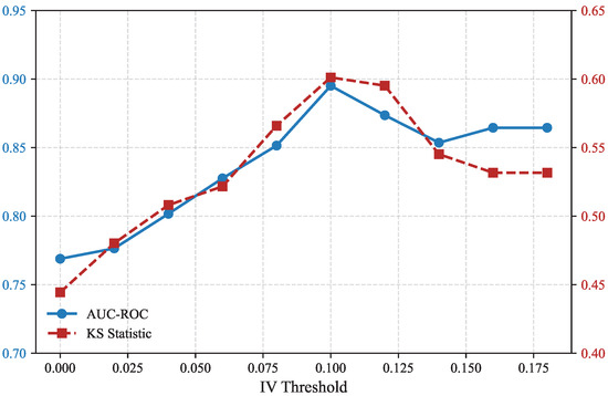
Figure 10.
IV threshold sensitivity analysis on the German Credit dataset.
Overall, the sensitivity results confirm that the proposed domain-constrained stacking framework maintains stable classification capability under varying IV selection rules. This robustness demonstrates that the model is not overly sensitive to specific threshold choices, ensuring its applicability across heterogeneous credit datasets.
Experiment V: Ablation Study on Feature Encoding Strategies. To further quantify the contribution of domain-informed feature transformations, an ablation study was conducted using both the GMSC and German Credit datasets. The experiment compared three configurations representing increasing levels of domain constraint: a baseline using raw numerical and label-encoded categorical variables, a version with unconstrained WOE transformation, and the proposed monotonic WOE encoding that enforces binning consistency with credit risk domain logic. All models were trained under the same stacking ensemble framework consisting of logistic regression, random forest, and XGBoost as base learners to ensure fair comparison.
As shown in Table 12, the domain-constrained monotonic WOE encoding consistently achieved the best predictive performance across both datasets. For the GMSC dataset, the AUC improved from 0.8450 to 0.8725 and the KS statistic increased from 0.5594 to 0.5879, demonstrating a clear enhancement in discriminatory power. Similarly, for the German Credit dataset, the AUC increased from 0.8849 to 0.8951 and the KS statistic rose from 0.5603 to 0.6012. These consistent improvements confirm that incorporating domain knowledge through monotonic binning not only strengthens interpretability but also enhances model generalization and stability. Overall, the ablation results validate that the domain-constrained feature transformation serves as a critical component of the proposed framework, bridging traditional credit scoring principles with modern ensemble learning.
Table 12.
Ablation study of different feature encoding strategies on two datasets.
4.6. Discussion
Overall, the experimental results across both benchmark datasets demonstrate that the proposed domain-constrained stacking framework achieves a well-balanced trade-off between predictive accuracy, interpretability, and computational efficiency. The Stacking Ensemble consistently outperforms individual base learners in terms of AUC–ROC, F1-Score, and KS statistics, indicating its superior discriminative power in identifying default risks. Notably, the relatively narrow confidence intervals across all experiments confirm the statistical reliability of the results. The ablation study further verifies that the domain-constrained monotonic WOE encoding contributes substantially to both model stability and generalization, bridging traditional credit risk principles with data-driven ensemble learning. Together, these findings substantiate the framework’s ability to integrate linear and nonlinear modeling paradigms into a unified, interpretable pipeline suitable for real-world credit scoring applications.
In addition to empirical performance, the proposed framework also reflects several characteristics valued in real-world financial governance. Although regulatory compliance was not the primary design objective, its emphasis on interpretability and decision traceability aligns well with the transparency principles highlighted in regulatory guidelines such as Basel II/III and GDPR. Strengthening this alignment through further methodological refinement would contribute to more transparent and accountable credit risk modeling practices.
Beyond quantitative performance, these results also invite broader reflections on fairness and responsible modeling. Although the WOE transformation provides a transparent and monotonic feature encoding scheme, correlated predictors may still act as proxies for sensitive attributes such as age, gender, or marital status, thereby introducing unintended biases into decision outcomes. Such risks echo recent literature emphasizing fairness-aware credit scoring and algorithmic accountability [39,48,49]. Embedding bias detection or mitigation mechanisms within interpretable modeling frameworks thus represents an important step toward regulatory compliance and socially equitable credit risk assessment. Finally, it is worth noting that the proposed framework has the potential to be integrated into existing banking credit evaluation workflows. Owing to its modular structure and reliance on interpretable feature transformations, such as WOE and IV-based encoding, it can align with the rule-based components commonly adopted in financial institutions. This potential integration would allow the framework to enhance analytical precision while maintaining consistency with practical decision-making processes.
5. Conclusions
This study addressed the problem of credit default prediction by developing a domain-constrained ensemble framework that systematically integrates exploratory analysis, industry-informed pre-processing, and advanced machine learning. Through an extensive investigation of the datasets, exploratory data analysis (EDA) was conducted to uncover distributional characteristics, class imbalance, and irregularities across eleven variables. Guided by these findings, pre-processing strategies were implemented, including outlier removal, missing-value treatment, and label redefinition. To further align with industry practice and enhance statistical rigor, feature transformation was performed using binning, Weight-of-Evidence (WOE) encoding, and Information Value (IV) evaluation, yielding a structured feature space suitable for both interpretable and data-driven models. On this foundation, four complementary classifiers were constructed—logistic regression, random forest, XGBoost, and a stacking ensemble integrating both. Logistic regression provided a transparent and stable baseline, while random forest and XGBoost captured nonlinear dependencies and interactions. The stacking ensemble leveraged the strengths of these approaches within a two-layer architecture, combining their outputs through a meta-level logistic regression to achieve superior predictive performance compared with individual models, as evidenced by improvements in AUC, KS, and related metrics.
In addition to empirical improvements, the framework helps bridge traditional scorecard methodologies with modern predictive analytics. By embedding domain-informed feature preparation within an ensemble pipeline, it aligns better with real-world business practices while enhancing model generalization. Overall, the results indicate that credit default prediction can benefit from approaches that integrate established industry experience with the predictive strengths of machine learning. Future research could further strengthen the proposed framework by incorporating regularization-based learners (e.g., LASSO or Elastic Net) and stochastic imputation techniques to enhance generalization and preserve feature variability. Moreover, integrating unstructured data sources such as textual credit applications or behavioral transaction logs, together with pilot validation in collaboration with financial institutions, would help demonstrate its practicality and robustness in real-world credit decision systems.
Author Contributions
Conceptualization, M.-L.D. and Y.-L.M.; methodology, M.-L.D. and Y.-L.M.; software, Y.-L.M. and M.-L.D.; validation, M.-L.D., Y.-L.M. and F.-Q.Y.; formal analysis, M.-L.D. and F.-Q.Y.; investigation, Y.-L.M.; resources, M.-L.D.; data curation, M.-L.D. and Y.-L.M.; writing—original draft preparation, M.-L.D. and Y.-L.M.; writing—review and editing, F.-Q.Y.; visualization, F.-Q.Y.; supervision, Y.-L.M.; project administration, Y.-L.M.; funding acquisition, Y.-L.M. All authors have read and agreed to the published version of the manuscript.
Funding
This research was supported in part by the Liaoning Provincial Natural Science Foundation Joint Fund under Grant 2023-MSBA-080, and the National Natural Science Foundation of China under Grants 62002054 and 62072087.
Data Availability Statement
The original data presented in this study are openly available in public repositories. The GMSC dataset is available at Kaggle: Give Me Some Credit (https://www.kaggle.com/c/GiveMeSomeCredit, accessed on 25 September 2025), and the German Credit dataset is available at the UCI Machine Learning Repository: Statlog (German Credit Data) (https://archive.ics.uci.edu/dataset/144/statlog+german+credit+data, accessed on 25 September 2025).
Conflicts of Interest
The authors declare no conflicts of interest.
Appendix A. Exploratory Data Analysis and Pre-Processing on the German Credit Dataset
Appendix A.1. Dataset Overview
The exploratory data analysis (EDA) was conducted on the German Credit Data from the UCI Machine Learning Repository (https://archive.ics.uci.edu/dataset/144/statlog+german+credit+data, accessed on 25 September 2025), which contains 1000 loan applicants with 20 attributes and a binary target variable (Credit Risk, where one denotes “Good” and two denotes “Bad” clients). The dataset provides both demographic and financial indicators such as account status, credit history, savings, employment duration, and loan purpose. Each record represents one individual’s credit situation assessed by a German bank.
The dataset includes 13 categorical and 7 numerical features. Table A1 summarizes the numerical variables, while Figure A1, Figure A2, Figure A3 and Figure A4 present the categorical feature distributions.
Table A1.
Variable description of the German Credit Data dataset.
Table A1.
Variable description of the German Credit Data dataset.
| Variable Name | Type | Missing Values | Description |
|---|---|---|---|
| Attribute 1 | Categorical | no | Status of existing checking account |
| Attribute 2 | Integer | no | Duration |
| Attribute 3 | Categorical | no | Credit history |
| Attribute 4 | Categorical | no | Purpose |
| Attribute 5 | Integer | no | Credit amount |
| Attribute 6 | Categorical | no | Savings account/bonds |
| Attribute 7 | Categorical | no | Present employment since |
| Attribute 8 | Integer | no | Installment rate in percentage of disposable income |
| Attribute 9 | Categorical | no | Personal status and sex |
| Attribute 10 | Categorical | no | Other debtors/guarantors |
| Attribute 11 | Integer | no | Present residence since |
| Attribute 12 | Categorical | no | Property |
| Attribute 13 | Integer | no | Age |
| Attribute 14 | Categorical | no | Other installment plans |
| Attribute 15 | Categorical | no | Housing |
| Attribute 16 | Integer | no | Number of existing credits at this bank |
| Attribute 17 | Categorical | no | Job |
| Attribute 18 | Integer | no | Number of people being liable to provide maintenance for |
| Attribute 19 | Binary | no | Telephone |
| Attribute 20 | Binary | no | Foreign worker |
| class | Binary | no | 1 = Good, 2 = Bad |
Appendix A.2. Target Distribution
The distribution of the target variable is illustrated in Figure A1. Among the 1000 samples, approximately 70% are labeled as “Good” and 30% as “Bad” credit risk cases, indicating a moderate class imbalance, which was addressed using an oversampling technique during data pre-processing.

Figure A1.
Distribution of credit risk categories in the German Credit dataset.
Figure A1.
Distribution of credit risk categories in the German Credit dataset.

Appendix A.3. Categorical Feature Analysis
Thirteen categorical variables describe applicants’ qualitative characteristics such as checking account status, credit history, purpose of the loan, and housing situation. Each categorical attribute was mapped from encoded values (A11, A12, A13, etc.) to semantically meaningful labels.

Figure A2.
Distributions of the first six categorical features (Status of checking account, Credit history, Purpose, Savings account/bonds, Employment since, Personal status and sex).
Figure A2.
Distributions of the first six categorical features (Status of checking account, Credit history, Purpose, Savings account/bonds, Employment since, Personal status and sex).


Figure A3.
Distributions of the next six categorical features (Other debtors/guarantors, Property, Other installment plans, Housing, Job, Telephone).
Figure A3.
Distributions of the next six categorical features (Other debtors/guarantors, Property, Other installment plans, Housing, Job, Telephone).


Figure A4.
Distribution of the last categorical feature: Foreign worker.
Figure A4.
Distribution of the last categorical feature: Foreign worker.

From the categorical feature analysis, several notable patterns were observed. Applicants who have no checking account or maintain a higher balance (≥200 DM) generally demonstrate lower default rates, suggesting that individuals with better liquidity or rational spending habits tend to be more creditworthy. In contrast, those with adverse credit histories—such as delayed or critical accounts—exhibit a higher likelihood of default. Regarding loan purposes, car-related financing constitutes the largest share of credit applications and is associated with a slightly elevated default tendency compared to household or education loans. Furthermore, applicants with savings account balances below 100 DM display a markedly higher default risk, consistent with limited financial reserves. Stable employment status (≥4 years) and home ownership also correlate positively with good credit performance, highlighting the importance of financial stability and asset ownership in risk assessment.
Appendix A.4. Numerical Feature Analysis
Seven numerical variables (duration in month, credit amount, installment rate, residence since, age, number of credits, number of dependents) were analyzed using histograms and descriptive statistics.
Figure A5 shows the probability density distributions for good and bad clients. In the analysis of numerical features, similar insights emerge. Shorter loan durations (less than 30 months) are dominated by good clients, while extended repayment periods correspond to increased default probabilities. The distribution of credit amounts exhibits right-skewness, where smaller loan sizes are associated with lower risk, whereas larger credits entail higher financial exposure and greater default tendencies. Additionally, age demonstrates a clear behavioral pattern: younger clients, particularly those under 30 years old, show a higher propensity to default, which may reflect limited borrowing experience and unstable income. These observations collectively underline the relevance of both demographic and financial characteristics in shaping credit risk profiles.

Figure A5.
Distribution of numerical features by credit risk category. Blue and red lines represent the distributions of good and bad credit clients, respectively.
Figure A5.
Distribution of numerical features by credit risk category. Blue and red lines represent the distributions of good and bad credit clients, respectively.

Table A2 reports descriptive statistics (mean, standard deviation, and quartiles) and group-wise averages for good and bad users. These statistics reveal that bad users tend to have higher average credit amounts and slightly longer durations.
Table A2.
Statistical summary of numerical variables.
Table A2.
Statistical summary of numerical variables.
| Statistic | Duration | Credit Amt. | Inst. Rate (%) | Res. Time (yrs) | Age | Num. Credits | Maint. People |
|---|---|---|---|---|---|---|---|
| Count | 1000 | 1000 | 1000 | 1000 | 1000 | 1000 | 1000 |
| Mean | 20.90 | 3271.26 | 2.97 | 2.85 | 35.55 | 1.41 | 1.16 |
| Std | 12.06 | 2822.74 | 1.12 | 1.10 | 11.38 | 0.58 | 0.36 |
| Min | 4.00 | 250.00 | 1.00 | 1.00 | 19.00 | 1.00 | 1.00 |
| 25% | 12.00 | 1365.50 | 2.00 | 2.00 | 27.00 | 1.00 | 1.00 |
| Median | 18.00 | 2319.50 | 3.00 | 3.00 | 33.00 | 1.00 | 1.00 |
| 75% | 24.00 | 3972.25 | 4.00 | 4.00 | 42.00 | 2.00 | 1.00 |
| Max | 72.00 | 18,424.00 | 4.00 | 4.00 | 75.00 | 4.00 | 2.00 |
| Good Mean | 19.21 | 2985.46 | 2.92 | 2.84 | 36.22 | 1.42 | 1.16 |
| Bad Mean | 24.86 | 3938.13 | 3.10 | 2.85 | 33.96 | 1.37 | 1.15 |
| Mean Diff (Bad–Good) | 5.65 | 952.67 | 0.18 | 0.01 | −2.26 | −0.06 | −0.00 |
Appendix A.5. Data Pre-Processing
The German Credit Data required only minimal pre-processing before model training. All variables were verified to be complete, with no missing values or invalid entries identified during exploratory analysis. No extreme outliers were observed, and thus no trimming or transformation was necessary. To mitigate the moderate imbalance between the “Good” and “Bad” credit classes (approximately 70% vs. 30%), the Synthetic Minority Over-sampling Technique (SMOTE) was applied to the training set. This procedure effectively balanced the class distribution and ensured adequate representation of both credit risk categories during model learning.
References
- Fuster, A.; Goldsmith-Pinkham, P.; Ramadorai, T.; Walther, A. Predictably Unequal? The Effects of Machine Learning on Credit Markets. J. Financ. 2022, 77, 5–47. [Google Scholar] [CrossRef]
- Anderson, R. The Credit Scoring Toolkit: Theory and Practice for Retail Credit Risk Management and Decision Automation; Oxford University Press: Oxford, UK, 2007. [Google Scholar] [CrossRef]
- Beninel, F.; Bouaguel, W.; Belmufti, G. Transfer learning using logistic regression in credit scoring. arXiv 2012, arXiv:1212.6167. [Google Scholar] [CrossRef]
- Lessmann, S.; Baesens, B.; Seow, H.V.; Thomas, L.C. Benchmarking State-of-the-Art Classification Algorithms for Credit Scoring: An Update of Research. Eur. J. Oper. Res. 2015, 247, 124–136. [Google Scholar] [CrossRef]
- Bellotti, T.; Crook, J. Support Vector Machines for Credit Scoring and Discovery of Significant Features. Expert Syst. Appl. 2009, 36, 3302–3308. [Google Scholar] [CrossRef]
- Khandani, A.E.; Kim, A.J.; Lo, A.W. Consumer credit-risk models via machine-learning algorithms. J. Bank. Financ. 2010, 34, 2767–2787. [Google Scholar] [CrossRef]
- Arik, S.Ö.; Pfister, T. TabNet: Attentive interpretable tabular learning. Proc. Aaai Conf. Artif. Intell. 2021, 35, 6679–6687. [Google Scholar] [CrossRef]
- Bussmann, N.; Giudici, P.; Marinelli, D.; Papenbrock, J. Explainable machine learning in credit risk management. Comput. Econ. 2021, 57, 203–216. [Google Scholar] [CrossRef]
- Chen, T.; Guestrin, C. XGBoost: A scalable tree boosting system. In Proceedings of the 22nd ACM SIGKDD International Conference on Knowledge Discovery and Data Mining, San Francisco, CA, USA, 13–17 August 2016; pp. 785–794. [Google Scholar] [CrossRef]
- Ke, G.; Meng, Q.; Finley, T.; Wang, T.; Chen, W.; Ma, W.; Ye, Q.; Liu, T.Y. LightGBM: A highly efficient gradient boosting decision tree. In Proceedings of the 31st International Conference on Neural Information Processing System, Long Beach, CA, USA, 4–9 December 2017; Volume 30. Available online: https://dl.acm.org/doi/10.5555/3294996.3295074 (accessed on 25 September 2025).
- Prokhorenkova, L.; Gusev, G.; Vorobev, A.; Dorogush, A.V.; Gulin, A. CatBoost: Unbiased boosting with categorical features. In Proceedings of the 32nd International Conference on Neural Information Processing Systems, Montreal, QC, Canada, 2–8 December 2018; Volume 31. Available online: https://dl.acm.org/doi/10.5555/3327757.3327770 (accessed on 25 September 2025).
- Breiman, L. Random forests. Mach. Learn. 2001, 45, 5–32. [Google Scholar] [CrossRef]
- Wolpert, D.H. Stacked generalization. In Proceedings of the Neural Networks; Elsevier: Amsterdam, The Netherlands, 1992; pp. 241–259. [Google Scholar] [CrossRef]
- Dietterich, T.G. Ensemble methods in machine learning. In International Workshop on Multiple Classifier Systems; Springer: Berlin/Heidelberg, Germany, 2000; pp. 1–15. [Google Scholar] [CrossRef]
- Ofori, K.S.; Fianu, E.; Omoregie, O.K.; Odai, N.A.; Oduro-Gyimah, F. Predicting credit default among micro borrowers in Ghana. Res. J. Financ. Account. 2014, 5, 1697–2222. [Google Scholar]
- Acquah, H.; Addo, J. Determinants of loan repayment performance of fishermen: Empirical evidence from Ghana. Cercet. Agron. Mold. 2011, 44, 89–97. [Google Scholar]
- Addisu, M. Micro-finance repayment problems in the informal sector in Addis Ababa. Ethiop. J. Bus. Dev. 2006, 1, 29–50. [Google Scholar]
- Bhandary, R.; Shenoy, S.S.; Shetty, A.; Shetty, A.D. Attitudes toward educational loan repayment among college students: A qualitative enquiry. J. Financ. Couns. Plan. 2023, 34, 281–292. [Google Scholar] [CrossRef]
- Hand, D.J.; Henley, W.E. Statistical classification methods in consumer credit scoring: A review. J. R. Stat. Soc. Ser. A Stat. Soc. 1997, 160, 523–541. [Google Scholar] [CrossRef]
- Maalouf, M. Logistic regression in data analysis: An overview. Int. J. Data Anal. Tech. Strateg. 2011, 3, 281–299. [Google Scholar] [CrossRef]
- Yeh, I.C.; Lien, C.h. The comparisons of data mining techniques for the predictive accuracy of probability of default of credit card clients. Expert Syst. Appl. 2009, 36, 2473–2480. [Google Scholar] [CrossRef]
- Cervantes, J.; Garcia-Lamont, F.; Rodríguez-Mazahua, L.; Lopez, A. A comprehensive survey on support vector machine classification: Applications, challenges and trends. Neurocomputing 2020, 408, 189–215. [Google Scholar] [CrossRef]
- More, A.; Rana, D.P. Review of random forest classification techniques to resolve data imbalance. In Proceedings of the 2017 1st International conference on intelligent systems and information management (ICISIM), Piscataway, NJ, USA, 5–6 October 2017; pp. 72–78. [Google Scholar] [CrossRef]
- Vanaja, S.; Rameshkumar, K. Performance analysis of classification algorithms on medical diagnoses—A survey. J. Comput. Sci. 2015, 11, 30–52. [Google Scholar] [CrossRef]
- Hamdi, M.; Mestiri, S.; Arbi, A. Artificial intelligence techniques for bankruptcy prediction of tunisian companies: An application of machine learning and deep learning-based models. J. Risk Financ. Manag. 2024, 17, 132. [Google Scholar] [CrossRef]
- Viswanathan, P.K.; Shanthi, S.K. Modelling credit default in microfinance—An indian case study. J. Emerg. Mark. Financ. 2017, 16, 246–258. [Google Scholar] [CrossRef]
- Netzer, O.; Lemaire, A.; Herzenstein, M. When words sweat: Identifying signals for loan default in the text of loan applications. J. Mark. Res. 2019, 56, 960–980. [Google Scholar] [CrossRef]
- Suhadolnik, N.; Ueyama, J.; Da Silva, S. Machine Learning for Enhanced Credit Risk Assessment: An Empirical Approach. J. Risk Financ. Manag. 2023, 16, 496. [Google Scholar] [CrossRef]
- Maehara, R.; Benites, L.; Talavera, A.; Aybar-Flores, A.; Muñoz, M. Predicting financial inclusion in peru: Application of machine learning algorithms. J. Risk Financ. Manag. 2024, 17, 34. [Google Scholar] [CrossRef]
- Ersoy, E.; Li, H.; Schaffer, M.E.; Szendrei, T. Stacking Regression for Time-Series, with an Application to Forecasting Quarterly US GDP Growth. In Optimal Transport Statistics for Economics and Related Topics; Ngoc Thach, N., Kreinovich, V., Ha, D.T., Trung, N.D., Eds.; Studies in Systems, Decision and Control; Springer: Cham, Switzerland, 2024; Volume 483, pp. 153–174. [Google Scholar] [CrossRef]
- Liu, X.; Yang, Q.; Yang, R.; Liu, L.; Li, X. Corn Yield Prediction Based on Dynamic Integrated Stacked Regression. Agriculture 2024, 14, 1829. [Google Scholar] [CrossRef]
- Chen, X.; Klusowski, J.M.; Tan, Y.S. Error Reduction from Stacked Regressions. arXiv 2023, arXiv:2309.09880. [Google Scholar] [CrossRef]
- Lundberg, S.M.; Lee, S.I. A unified approach to interpreting model predictions. In Proceedings of the 31st International Conference on Neural Information Processing Systems, NeurIPS, Long Beach, CA, USA, 4–9 December 2017; Volume 30. Available online: https://dl.acm.org/doi/10.5555/3295222.3295230 (accessed on 25 September 2025).
- Molnar, C. Interpretable Machine Learning: A Guide for Making Black Box Models Explainable; Christoph Molnar: Munich, Germany, 2022. [Google Scholar]
- Demajo, L.M. Explainable AI for Interpretable Credit Scoring. arXiv 2020, arXiv:2012.03749. [Google Scholar] [CrossRef]
- Bücker, M.; Szepannek, G.; Gosiewska, A.; Biecek, P. Transparency, Auditability and eXplainability of Machine Learning Models in Credit Scoring. arXiv 2020, arXiv:2009.13384. [Google Scholar] [CrossRef]
- Alonso, A.; Carbó, J.M. Accuracy of Explanations of Machine Learning Models for Credit Decision. 2022. Available online: https://www.bde.es/f/webbde/SES/Secciones/Publicaciones/PublicacionesSeriadas/DocumentosTrabajo/22/Files/dt2222e.pdf (accessed on 28 September 2025).
- Guan, C.; Suryanto, H.; Mahidadia, A.; Bain, M.; Compton, P. Responsible credit risk assessment with machine learning and knowledge acquisition. Hum.-Centric Intell. Syst. 2023, 3, 232–243. [Google Scholar] [CrossRef]
- Valdrighi, G.; M Ribeiro, A.; SB Pereira, J.; Guardieiro, V.; Hendricks, A.; Miranda Filho, D.; Nieto Garcia, J.D.; F Bocca, F.; B Veronese, T.; Wanner, L.; et al. Best practices for responsible machine learning in credit scoring. Neural Comput. Appl. 2025, 37, 20781–20821. [Google Scholar] [CrossRef]
- Komorowski, M.; Marshall, D.C.; Salciccioli, J.D.; Crutain, Y. Exploratory data analysis. In Secondary Analysis of Electronic Health Records; Springer: Cham, Switzerland, 2016; pp. 185–203. [Google Scholar] [CrossRef]
- Persson, R. Weight of Evidence Transformation in Credit Scoring Models: How Does It Affect the Discriminatory Power? Master’s Thesis, Lund University, Lund, Sweden, 2021. [Google Scholar]
- Zhang, L.; Ray, H.; Priestley, J.; Tan, S. A descriptive study of variable discretization and cost-sensitive logistic regression on imbalanced credit data. J. Appl. Stat. 2020, 47, 568–581. [Google Scholar] [CrossRef] [PubMed]
- Mironchyk, P.; Tchistiakov, V. Monotone optimal binning algorithm for credit risk modeling. Utr. Work Pap. 2017. [Google Scholar] [CrossRef]
- Fahner, G. Developing transparent credit risk scorecards more effectively: An explainable artificial intelligence approach. Data Anal. 2018, 2018, 17. [Google Scholar]
- Oliveira, I.; Chari, M.; Haller, S.; NC, C. SAS/OR: Rigorous constrained optimized binning for credit scoring. In Proceedings of the SAS Global Forum 2008 on Data Mining and Predictive Modeling, San Antonio, TX, USA, 16–19 March 2008. [Google Scholar]
- Navas-Palencia, G. Optimal binning: Mathematical programming formulation. arXiv 2020, arXiv:2001.08025. [Google Scholar] [CrossRef]
- Gal, Y.; Ghahramani, Z. Dropout as a bayesian approximation: Representing model uncertainty in deep learning. In Proceedings of the International Conference on Machine Learning. PMLR, New York, NY, USA, 19–24 June 2016; pp. 1050–1059. Available online: https://dl.acm.org/doi/10.5555/3045390.3045502 (accessed on 25 September 2025).
- Kleinberg, J.; Ludwig, J.; Mullainathan, S.; Rambachan, A. Algorithmic fairness. AEA Pap. Proc. 2018, 108, 22–27. [Google Scholar] [CrossRef]
- Moldovan, D. Algorithmic decision making methods for fair credit scoring. IEEE Access 2023, 11, 59729–59743. [Google Scholar] [CrossRef]


Disclaimer/Publisher’s Note: The statements, opinions and data contained in all publications are solely those of the individual author(s) and contributor(s) and not of MDPI and/or the editor(s). MDPI and/or the editor(s) disclaim responsibility for any injury to people or property resulting from any ideas, methods, instructions or products referred to in the content. |
© 2025 by the authors. Licensee MDPI, Basel, Switzerland. This article is an open access article distributed under the terms and conditions of the Creative Commons Attribution (CC BY) license (https://creativecommons.org/licenses/by/4.0/).