Abstract
Deep learning on graphs has emerged as a leading paradigm for intrusion detection, yet its performance in optical networks is often hindered by sparse labeled data and severe class imbalance, leading to an “under-reaching” issue where supervision signals fail to propagate effectively. To address this, we introduce Pseudo-Metapaths: dynamic, semantically aware propagation routes discovered on-the-fly. Our framework first leverages Beta-Wavelet spectral filters for robust, frequency-aware node representations. It then transforms the graph into a dynamic heterogeneous structure using the model’s own pseudo-labels to define transient ‘normal’ or ‘anomaly’ node types. This enables an attention mechanism to learn the importance of different Pseudo-Metapaths (e.g., Anomaly–Normal–Anomaly), guiding supervision signals along the most informative routes. Extensive experiments on four benchmark datasets demonstrate quantitative superiority. Our model achieves state-of-the-art F1-scores, outperforming a strong spectral GNN backbone by up to 3.15%. Ablation studies further confirm that our Pseudo-Metapath module is critical, as its removal causes F1-scores to drop by as much as 7.12%, directly validating its effectiveness against the under-reaching problem.
MSC:
68T07
1. Introduction
Modern global communications fundamentally depend on optical networks, which provide the high-capacity, long-haul infrastructure necessary to sustain today’s exponentially growing data demands [1,2,3,4]. Their continued advancement is not merely a technological imperative but a societal one, as they enable essential services—from broadband internet to the operation of national critical systems [5,6,7]. Yet, as these networks grow more intricate and indispensable, their role in transmitting sensitive, high-stakes information makes them prime targets for advanced cyber threats [8,9,10]. Attack vectors now extend beyond traditional service outages to include insidious physical-layer intrusions, jeopardizing both network reliability and broader security interests [10,11]. Consequently, fortifying the resilience and security of optical infrastructure against such adaptive—and often covert—adversarial tactics has emerged as a paramount challenge [11].
We select optical networks as the focal point of this study precisely because they create a “perfect storm” of challenges for intrusion detection, making them an ideal proving ground for advanced graph-based methods. Firstly, the high-stakes and critical nature of optical infrastructure demands extremely high reliability, meaning that successful intrusions are, by design, extremely rare events. This operational reality directly translates into datasets with severe class imbalance and sparse labels—the very conditions that cripple standard supervised learning models. Secondly, the sheer volume and speed of data transmission make traditional deep packet inspection infeasible, shifting the focus to relational and behavioral patterns among network devices. This naturally motivates modeling the system as a graph, where subtle, coordinated malicious activities can be identified. Therefore, fortifying optical networks necessitates a paradigm that can effectively learn from sparse, imbalanced relational data and propagate supervisory signals across vast topologies, which is the central challenge we address.
Recently, graph-based deep learning has become a compelling paradigm for intrusion detection. Communication systems can be naturally modeled as graphs where nodes represent network devices and edges capture traffic flows, control-plane associations, or physical-layer couplings. Graph Neural Networks (GNNs) excel at learning from such relational data, enabling context-aware detection that surpasses methods based on isolated features [12,13]. However, directly applying GNNs to real-world optical networks reveals critical limitations. The core challenge stems from the intersection of severe label sparsity—anomalies are inherently rare and expensive to annotate—and the need for supervision signals to propagate across vast, complex topologies [14].
This leads to a critical bottleneck we formalize as under-reaching: supervision signals from the few labeled nodes fail to effectively influence the predictions of distant, unlabeled nodes that may be semantically related. This issue is exacerbated by two intertwined phenomena. First, deep message-passing GNNs are hampered by over-smoothing and over-squashing, which respectively dilute discriminative features and create informational bottlenecks that prevent long-range signal transmission [15,16,17,18,19]. Second, intrusion patterns in optical networks frequently violate the homophily assumption [20,21], as malicious nodes often connect to predominantly benign neighborhoods. This heterophilous nature blunts the effectiveness of standard GNNs, which are optimized for homophilous connections [22,23,24].
Existing remedies address parts of this problem but are insufficient in isolation. Post hoc label propagation can improve local consistency but falters under the severe label scarcity [25,26]. Self-training with pseudo-labels amplifies supervision but risks propagating confirmation bias, especially under strong class imbalance [27,28,29,30]. On the representation side, spectral methods are adept at capturing high-frequency anomaly signatures but lack a mechanism to guide supervision along meaningful multi-hop routes [31,32]. Finally, while heterogeneous GNNs elegantly handle relational semantics, they require a predefined schema, which is absent in this dynamically evolving problem [33,34]. A unified framework that captures anomaly-specific signals while simultaneously learning where to propagate them remains a critical gap.
We address this gap by introducing Pseudo-Metapaths: dynamic, semantically aware propagation routes discovered on-the-fly. Our framework begins by using Beta-Wavelet spectral filtering to extract high-frequency components indicative of anomalies, producing robust initial node embeddings that are resilient to heterophily and local noise. The core of our innovation lies in then transforming the graph into a transiently heterogeneous structure. At each training epoch, we assign temporary “normal” or “anomaly” types to nodes using the model’s own pseudo-labels. This transformation enables an attention mechanism to automatically learn which Pseudo-Metapaths (e.g., ‘Anomaly–Normal–Anomaly‘) are most effective for conveying supervisory signals. By coupling high-frequency spectral cues with dynamic metapath attention, our framework delivers label information across semantically promising—not merely topologically adjacent—regions of the network, directly combating the under-reaching problem.
Our contributions are threefold:
- We introduce a formalization of the under-reaching problem for intrusion detection in optical networks, identifying its roots in the interplay of label sparsity, class imbalance, and network heterophily.
- We propose the concept of Pseudo-Metapaths—a novel mechanism to learn dynamic, pseudo-label-conditioned propagation channels. We integrate this into a framework with Beta-Wavelet filtering to both capture and intelligently route anomaly signals.
- We provide extensive empirical validation demonstrating that our method consistently outperforms remarkable GNNs and specialized graph anomaly detection techniques, showcasing superior robustness and long-range supervision propagation.
2. Background
Optical networks inherently exhibit a graph structure, where network devices can be naturally represented as nodes and their interconnections as edges. This structural correspondence makes Graph Neural Networks (GNNs) a compelling choice for intrusion detection, as they leverage message passing to capture relational dependencies that are invisible to traditional, feature-based models [12]. By aggregating information from local neighborhoods, GNNs learn contextualized representations that reflect both node attributes and topological context. This formulation situates the problem within the broader field of graph anomaly detection (GAD), which aims to identify nodes, edges, or subgraphs that deviate significantly from expected behavioral or structural patterns [31]. At its core, GAD relies on the principle that anomalies manifest as statistical or structural outliers in the graph [35].
However, applying this paradigm to intrusion detection in optical networks introduces significant practical challenges. Unlike typical GAD settings, security-related anomalies in optical infrastructures are not only rare and difficult to label but also exhibit complex, non-localized patterns that strain the assumptions and mechanisms of standard GNNs. Two interdependent issues stand out: the heterophilous nature of malicious activity and the limited capacity of GNNs to propagate supervision effectively across sparse and unbalanced graphs.
One major challenge is heterophily, where malicious nodes frequently reside in neighborhoods dominated by benign entities [35]. This contradicts the homophily bias embedded in most conventional GNN architectures, which assume that connected nodes are likely to share similar labels or features. As a result, these models tend to average out anomalous signals during neighborhood aggregation, leading to the suppression or complete loss of critical evidence [22]. In such scenarios, anomalies become harder to distinguish.
To mitigate this limitation, recent research has increasingly turned to spectral graph theory. Wavelet-based frameworks offer a powerful means to isolate specific frequency components of graph signals, thereby amplifying high-frequency patterns that are often indicative of anomalous behavior [24,36]. Several state-of-the-art methods have built upon this principle [37]. For example, BWGNN [38] employs Beta kernels to construct adaptive, localized band-pass filters specifically tuned for high-frequency anomalies. AMNet [39] integrates signals across multiple frequency bands to enrich node representations, while BernNet [40] leverages Bernstein polynomials to achieve more expressive and flexible spectral filtering. Although these approaches excel at capturing the spectral signatures of anomalies, they do not inherently address the challenge of propagating such discriminative information effectively across the graph, especially when supervision is limited to only a few labeled nodes.
Another remaining core bottleneck rooted in the GNN’s message-passing mechanism itself. Constrained to propagate information strictly along the graph’s explicit edges, standard GNNs are prone to over-smoothing, where node representations become indistinguishable after multiple hops, and over-squashing, where rich signals are compressed through narrow structural bottlenecks [17,18,41]. The consequences of these propagation issues are significantly exacerbated in domains such as intrusion detection, which suffer from sparse labels and severe class imbalance. In such challenging settings, this confluence of factors gives rise to what we term the under-reaching problem: supervision signals from the few labeled anomalies are too attenuated to effectively influence distant yet semantically relevant nodes [42,43]. Given the topological sparsity of malicious entities, critical discriminative cues must often traverse long, multi-hop paths, a task for which conventional message passing is fundamentally ill-suited, which is the central concern of this paper.
3. Preliminary
In this section, we introduce some necessary concepts used in this paper.
3.1. Heterogeneous Graph and Metapath
Much real-world data can be effectively represented as Heterogeneous Graphs (HeteGs). In contrast to homogeneous graphs, HeteGs encompass multiple types of nodes and edges, each conveying rich information and forming a complex topological structure. Motivated by the need to analyze such data, various well-performing Heterogeneous Graph Neural Networks (HeteGNNs) have been proposed [44,45]. HeteGNNs often adopt a metapath-centric framework to integrate the diverse attributes inherent in HeteGs. The core concept involves utilizing metapaths to semantically aggregate nodes that are distantly located from each other [44]. For example, as shown in Figure 1, with the metapath paper-author-paper, paper-typed node-P0 and {P4,5,6} can be viewed as neighbors directly while ignoring author-typed node-A2. Unlike traditional GNNs, which directly aggregate messages from adjacent nodes, most HeteGNNs employ a concept known as metapaths.

Figure 1.
HeteGNNs have two typical working steps: (1) Collect info in a specific metapath context. (2) Fuse the collected info and produce predictions. For example, with the metapath paper(P)-author(A)-paper(P), the features on paper-typed node-P0 can be propagated to paper-typed node-{P4,5,6} directly while ignoring author-typed node-A2.
3.2. Spectral Graph Processing
By treating the features on nodes as signals, regarding the smoothness of the signals as frequency, and associating it with the eigenvalues of the graph’s Laplacian matrix, spectral graph methods provide an alternative but effective aspect for graph data processing distinct from the topological domain [46,47].
An undirected and unweighted graph comprising N vertices can be formally described as . When we consider the features associated with each node, we denote the graph as , where X represents the node feature matrix. This distinction allows us to first discuss the topological properties and subsequently incorporate the node-level signal information required for our spectral analysis and GNN model, with V representing the set of vertices and E the collection of edges. The structure is encoded in the adjacency matrix . To analyze graph signals spectrally, we utilize the Laplacian matrix defined as , where the diagonal matrix D has entries . Given that L exhibits real, symmetric, and positive semi-definite properties, it can be factorized as . Here, U encompasses the eigenvectors while represents eigenvalues arranged in ascending order (). The eigenvectors contained in U constitute the Graph Fourier Basis, with eigenvalues corresponding to graph frequencies [48].
For a signal defined on the graph, its smoothness metric is expressed by Equation (1):
with . This formulation reveals that signal components associated with smaller eigenvalues exhibit smoother (lower-frequency) variations across the graph, whereas those linked to larger eigenvalues manifest higher-frequency fluctuations. The Graph Fourier Transform (GFT) facilitates spectral processing through , where functions as a component-wise filter in the spectral domain.
3.3. Graph Spectral Wavelet and Its Chebyshev Approximation
The Graph Wavelet Transform is constructed from two fundamental elements: a scaling function and a set of wavelet kernels. For any given scale , the wavelet kernel is formulated as an operator , and similarly, the scaling function is defined as the operator .
Direct computation of these transforms is often impractical for large graphs due to the high computational cost of eigen-decomposition, which scales cubically with the number of nodes (). To circumvent this bottleneck, a common strategy is to employ Chebyshev polynomial expansion to approximate the operators and . A prerequisite for applying Chebyshev approximation to a function is that its input domain must be confined to the interval . To meet this requirement, it is advantageous to utilize the normalized graph Laplacian, which is defined as
where D represents the diagonal degree matrix () and A is the adjacency matrix. The eigenvalues of this normalized Laplacian are guaranteed to fall within the range , a property that facilitates the necessary rescaling for the approximation of and . For the remainder of this paper, unless otherwise specified, the eigen-decomposition will refer to that of the normalized Laplacian
Both the wavelet kernels and the scaling function can be approximated using this polynomial expansion. For notational convenience, we can consolidate these operators into a single matrix:
As established in [36], these approximations, denoted as and , are formulated using a truncated Chebyshev series of order Z:
where represents the z-th order Chebyshev polynomial evaluated at the normalized Laplacian . These polynomials are generated via the recurrence relation:
with initial conditions and . The corresponding Chebyshev coefficients, and , are determined by the following integrals:
The resulting approximated transform operator can be written as
An important property of this transform is the Parseval tight frame condition, which is met if for all eigenvalues . When this condition holds, the transform is energy-preserving. This is typically realized by carefully choosing kernel functions, such as those from the Meyer or Mexican hat families. In cases where the tight frame property is not satisfied, signal reconstruction requires the Moore–Penrose pseudoinverse of the operator, , which is calculated as
Consequently, for a given signal on the graph, its wavelet coefficients are , and the signal can be reconstructed via the inverse transform:
where the operator has dimensions , while its pseudoinverse has dimensions , with N representing the total number of graph nodes.
The primary advantage of the Chebyshev approximation lies in its computational efficiency. For a graph comprising N nodes and E edges, a Z-order polynomial approximation requires a series of matrix-vector multiplications involving the sparse Laplacian matrix. This process has a computational cost of . Given that Z is a small constant (typically between 10 and 50) that does not depend on the graph size N, and for sparse graphs where E is often proportional to N, the overall complexity is nearly linear. This makes the method significantly more scalable and tractable for large-scale graphs than the computationally prohibitive complexity associated with direct eigen-decomposition.
It is important to acknowledge that the explicit computation of the graph Laplacian’s eigen-decomposition has a theoretical complexity of , which can be prohibitive for very large graphs. However, for the small-to-medium-scale datasets considered in our experiments (where the number of nodes ), this direct spectral approach remains computationally feasible. Thanks to modern hardware acceleration, particularly CUDA-enabled GPUs such as the NVIDIA H800, the practical execution time for this operation is well within an acceptable range for typical research workflows. Therefore, we adopt the direct eigen-decomposition method in our current framework for its precision. The exploration of approximation techniques to enhance scalability for larger graphs, such as the Chebyshev polynomial expansion, is deferred as a direction for future work.
3.4. Spectral Properties of Anomaly Signals: Anomalies as High-Frequency Components
A foundational challenge in applying GNNs to anomaly detection is that many conventional architectures, such as GCN, implicitly function as low-pass filters. By design, they smooth signals across neighborhoods, which is effective under the homophily assumption but counterproductive for anomaly detection. Anomalies, by definition, represent significant deviations from the norm, introducing sharp, localized changes into the graph signal. These abrupt variations are fundamentally high-frequency phenomena. The seminal work by Tang et al. [38] provides a rigorous spectral analysis of this behavior, mathematically proving a key characteristic: the presence of anomalies causes the signal’s spectral energy to concentrate in the high-frequency domain. To understand this, we delve into their theoretical framework. To formalize the analysis, given an unweighted, undirected homogeneous graph, we assume its node features (the signal) are drawn from a multivariate Gaussian distribution:
where is the mean vector (with being an all-ones vector) and is the variance. In this model, the degree of anomaly is quantified by the coefficient of variation, . A larger variance or a smaller absolute mean signifies greater deviation among node features, thus representing a more pronounced anomalous state in the overall graph signal.
3.4.1. Signal Analysis in the Spectral Domain
The analysis transitions from the spatial domain to the spectral domain via the Graph Fourier Transform (GFT), . Due to the rotational invariance of the Gaussian distribution, the transformed signal is also Gaussian: .
A crucial insight lies in the structure of . For a connected, undirected graph, the all-ones vector is the eigenvector corresponding to the smallest eigenvalue . Consequently, the vector is non-zero only at its first component, i.e., . This implies that the distributions of the spectral coefficients are not identical:
- The first spectral coefficient (the DC component) follows a non-central distribution: .
- All other coefficients (the AC components) are centered at zero: for .
This decomposition is key: the signal’s mean primarily influences the lowest frequency, while its variance—and thus, its anomalous nature—is captured by the higher frequencies.
3.4.2. Mathematical Proof of Increased High-Frequency Energy
To quantify how energy is distributed across frequencies, Tang et al. [38] introduce the low-frequency energy ratio:
which measures the proportion of signal energy within the first k lowest frequencies. The goal is to show that as the anomaly degree increases, decreases.
To achieve this, the Proposition 2 in [38] demonstrates that the expected inverse of this ratio, , is monotonically increasing with the anomaly degree . The logic is as follows: the term can be expressed as . By normalizing with and letting , we have and for . The expectation becomes dependent on the term . The sum follows a central chi-squared distribution, but follows a non-central chi-squared distribution whose non-centrality parameter is related to . The core of the proof is realizing that as the anomaly degree increases, the non-centrality parameter for decreases. This reduces the expected value of . A smaller denominator leads to a larger value for the entire expectation .
This chain of reasoning mathematically confirms that a higher degree of anomaly leads to a smaller proportion of energy in the low-frequency spectrum. Since the low-frequency and high-frequency energy components must add up to the total signal energy, a decrease in the proportion of low-frequency energy directly implies a corresponding increase in the proportion of high-frequency energy. This provides a strong theoretical justification for our approach: to effectively detect intrusions, it is not just beneficial but necessary to employ a mechanism capable of capturing these high-frequency spectral signatures. This motivates our choice of the Beta-Wavelet module, which is explicitly designed as a set of learnable band-pass filters, making it exceptionally well-suited to isolate the discriminative high-frequency components that characterize anomalous activities.
Discussion
To further justify our spectral approach, we contrast it with methods that rely on purely topological features. The key distinction lies in the nature of the anomalies we aim to detect: they manifest as high-frequency signals rather than distinctive topological structures. Consequently, a purely structural approach, such as one based on graph domination, would fail in two key scenarios:
- Camouflaged Anomalies: A node with a highly anomalous feature vector (a large deviation in its signal, leading to a large ) could be located in a structurally unremarkable part of the graph (e.g., low centrality, not part of a minimal dominating set). A structural method would miss it, whereas spectral filtering is designed to detect such high-frequency variations.
- Structural Outliers with Normal Behavior: A node could be a structural outlier (e.g., a bridge node, high centrality) but exhibit perfectly normal features. Its signal would be similar to its neighbors, resulting in a low . A structural parameter might flag it as important or suspicious, while spectral analysis would correctly identify its signal as low-frequency (smooth) and thus non-anomalous.
Therefore, while structural parameters are valuable for understanding graph topology, they are mathematically ill-equipped to detect anomalies defined by signal characteristics. The spectral approach, by its very formulation, is designed to analyze this crucial signal-structure relationship, making it the more appropriate and powerful choice for our task.
4. Methodology
Our proposed framework, PseudoMetapathNet, tackles the under-reaching problem in graph-based intrusion detection by creating and leveraging dynamic, semantically aware propagation routes. In contrast to methods that augment graph structures topologically, our approach learns to route supervision signals along “Pseudo-Metapaths” that are most informative for identifying anomalies. The entire process can be broken down into three main stages: (a) learning robust, frequency-aware node representations using Beta-Wavelet spectral filters; (b) dynamically transforming the graph into a pseudo-heterogeneous structure based on the model’s evolving predictions; and (c) propagating information via an attention mechanism that learns the importance of different Pseudo-Metapaths. Figure 2 provides a schematic overview of our framework.
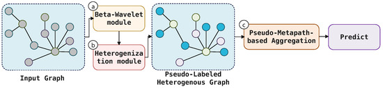
Figure 2.
An illustration of our proposed framework. (a) The Beta-Wavelet module generates initial node embeddings. (b) Based on pseudo-labels from the model, the graph is dynamically heterogenized with ‘Normal’ (N) and ‘Anomaly’ (A) node types. (c) An attention mechanism learns the importance of different Pseudo-Metapaths (e.g., A-N-A) to guide the aggregation of information and produce the final predictions, effectively mitigating the under-reaching issue.
We detail these three stages in the following three subsections.
4.1. Beta-Wavelet-Based Graph Representation Learning
As spectral graph theory suggests, anomalies often manifest as high-frequency signals relative to their local neighborhoods. To effectively isolate these discriminative spectral signatures, our framework is built upon a spectral GNN backbone. We specifically select a model inspired by the Beta-Wavelet Graph Neural Network (BWGNN) [38], leveraging its proven ability to construct precise, tunable band-pass filters ideal for graph-based anomaly detection (GAD).
The filter’s design is grounded in the scaled Beta kernel function, which provides mathematical control over its spectral response. This function is expressed as
where , and represents a scaled eigenvalue from the graph spectrum. As detailed in the work of Tang et al. [38], the two parameters, p and q, allow for precise control over the filter’s central frequency and bandwidth, analogous to the mean and variance of a Beta distribution.
First, the filter’s central frequency (), where its response is maximal, is determined by the ratio of p to q:
To target high-frequency signals, which correspond to the largest eigenvalues of the graph Laplacian (approaching 2), we can simply set . This ensures the filter is most sensitive to the spectral bands where anomaly signatures typically reside. Second, the filter’s bandwidth, or precision, is controlled by its variance ():
As the polynomial order increases, the variance approaches zero, concentrating the filter’s energy around its central frequency . This transforms it into a highly selective, narrow band-pass filter, crucial for distinguishing anomalous patterns from other innocuous high-frequency noise. In essence, by tuning p and q, we can engineer a filter that is both centered on the high-frequency regions and highly selective in its response.
This kernel is used to construct a family of wavelet base filters, which together form the multi-scale filter of our representation learning module . Each wavelet filter matrix, representing a specific instance of the general graph wavelet operator discussed previously, is defined as
The complete filtering operation on a d-dimensional input signal then produces an initial set of node embeddings , as defined in Equation (17):
where is the normalized graph Laplacian with eigen-decomposition .
While these initial embeddings are effective at capturing intrinsic node characteristics, relying solely on this module for prediction suffers from the “under-reaching” issue: the supervision signal from the few labeled nodes cannot effectively propagate to distant unlabeled nodes. This limitation motivates the subsequent steps of our methodology. It is also worth noting that our framework is modular. While we select BWGNN as a powerful spectral backbone, other GNNs adept at capturing high-frequency signals, such as ACM-GNN [49] or FAGCN [50], could serve as alternative feature extractors. As our experiments will demonstrate, the most significant performance gains stem from our novel propagation mechanism, which is agnostic to the specific choice of the initial encoder.
4.2. Dynamic Graph Heterogenization
To overcome the propagation limits of standard GNNs and enable more sophisticated, semantically driven message passing, we introduce a novel step: dynamic graph heterogenization. The core idea is to temporarily impose a heterogeneous structure onto the natively homogeneous graph, allowing us to leverage powerful semantic aggregation via metapaths.
This transformation is achieved dynamically at each training iteration k. First, using the node representations generated by the Beta-Wavelet module, the model computes a preliminary set of predictions (i.e., pseudo-labels) for all nodes. A node v is assigned a temporary type based on its predicted probability of being an anomaly:
where is a confidence threshold. This process transforms the input homogeneous graph G into a transient, pseudo-heterogeneous graph , where is the set of temporary node types .
Crucially, this heterogenization is not static. The node types are recalculated at every training step, evolving as the model’s understanding of the graph improves. This dynamic nature allows the model to self-correct and progressively refine the semantic structure it uses for information propagation, preventing early-stage prediction errors from causing permanent damage.
4.3. Propagating via Learnable Pseudo-Metapaths
With the dynamically induced heterogeneous structure, we propose a mechanism to automatically learn optimal composite Pseudo-Metapaths in an on-the-fly fashion. Specifically, we generate new adjacency matrices representing useful multi-hop relations and then perform propagations on these learned Pseudo-Metapaths.
First, based on the node types in , we define a set of candidate adjacency matrices . This set includes matrices for each possible pseudo-relation type:, namely , where if there is an edge from node j of type to node i of type . To learn variable-length metapaths, we also include the identity matrix I in this set.
A layer inspired by the Graph Transformer Network (GTN) [51] is then used to learn a soft selection of these candidate matrices. Specifically, we introduce a learnable weight vector , which is implemented as the kernel of a convolution. Each element in corresponds to a candidate matrix in the set . Applying a softmax function to this vector yields a normalized attention vector, , where each element represents the learned importance of the corresponding candidate matrix . These attention scores are then used to compute a weighted combination of the candidate matrices, forming a new graph structure , as expressed in Equation (19):
The resulting matrix represents a new graph structure defined by a weighted combination of the base pseudo-relations.
To discover longer and more complex Pseudo-Metapaths, we stack K GT layers. The output of the k-th layer, , is generated by multiplying the output of the previous layer with a new learned combination of base matrices. This composition allows the model to construct metapaths of up to length K, expressed as Equation (20):
To learn multiple distinct Pseudo-Metapaths simultaneously, we extend this operation to have channels.
Finally, we perform graph convolution on these newly generated graphs. For each learned metapath graph , we apply a GNN layer (e.g., GCN) to propagate information from the concatenated representations , where denotes the feature concatenation operator. This process can be expressed as Equation (21):
where , is its degree matrix, and W is a shared trainable weight matrix. The final, semantically enriched representation for each node, , is obtained by aggregating the outputs from all channels, as shown in Equation (22):
This final representation is then used for the ultimate intrusion detection prediction. By learning to construct the most salient propagation pathways automatically, our framework establishes powerful, long-range information highways that directly and effectively combat the under-reaching problem.
In contrast to fixed schemas, our work dynamically induces pseudo-types from model predictions and learns to route supervision along Pseudo-Metapaths, coupling frequency-aware representations with adaptive, semantically guided propagation to mitigate under-reaching in low-label, imbalanced, and heterophilous regimes.
The pseudo-code of the forward process of PseudoMetapathNet is shown in Algorithm 1, and the PseudoMetapathNet framework is trained end-to-end by optimizing a composite loss function. This objective is carefully designed to address two distinct but interconnected goals: (1) ensuring high accuracy on the final intrusion detection task and (2) regularizing the intermediate dynamic graph heterogenization stage to produce a coherent and meaningful semantic structure. To this end, our total loss function is composed of a primary supervised task loss and a self-supervised auxiliary contrastive loss .
| Algorithm 1 PseudoMetapathNet (Forward Process) |
|
4.3.1. Primary Task Loss
The primary objective is to correctly classify nodes as either normal or anomalous. This is achieved through a standard supervised learning setup. Given the final semantically enriched node representations from Equation (22), a final linear classifier is applied to produce the prediction logits. For the set of labeled training nodes, denoted as , we have
where is the true label for node v, and is the predicted probability of node v being an anomaly, derived from . This loss directly drives the model to learn effective Pseudo-Metapaths for the downstream task. Here, is a binary cross-entropy (BCE) loss, which is equivalent to the negative log-likelihood (NLL) of the predictions. The standard cross-entropy (CE) loss can also be adopted according to the dataset. The negative sign is necessary as the log-likelihood (the term inside the summation) is non-positive, and the training objective is to minimize this loss (i.e., maximize the likelihood). The formulation is numerically stable at boundary conditions: for a perfect prediction (e.g., ), the loss correctly evaluates to 0, as the term’s limit is 0.
4.3.2. Auxiliary Contrastive Loss for Stable Heterogenization
A critical challenge in our framework is that the quality of the learned Pseudo-Metapaths is highly dependent on the stability and semantic coherence of the pseudo-labels generated. Relying solely on the distant supervision from can lead to unstable training, as the pseudo-labeling process lacks a direct, immediate learning signal.
To address this, we introduce an auxiliary self-supervised loss, , which acts as a regularization term on the initial node embeddings . The goal of this loss is to enforce a more structured embedding space, providing a strong inductive bias for the dynamic heterogenization stage. Specifically, it encourages the representations of nodes that are assigned the same pseudo-type to be closer to each other, while pushing apart the representations of nodes with different pseudo-types.
We formulate this as a contrastive loss. For a given pair of nodes , we define their relationship based on their pseudo-labels and from Equation (18). The loss is defined over a batch of randomly sampled node pairs and consists of two components:
where is the initial embedding of node , is the squared Euclidean distance, is the indicator function, and m is a positive margin hyper-parameter. This loss minimizes the distance between positive pairs (nodes with the same pseudo-type) and enforces that negative pairs (nodes with different pseudo-types) are separated by at least the margin m. This provides a direct supervisory signal to the Beta-Wavelet module, ensuring it produces embeddings that are not only spectrally discriminative but also well-clustered according to the model’s own evolving semantic understanding.
4.3.3. Overall Objective
The final training objective is a weighted combination of the task loss and the auxiliary loss, controlled by a balancing hyperparameter :
By optimizing this composite objective, PseudoMetapathNet learns to simultaneously perform the classification task and refine its own internal representation of the graph’s semantic structure. This dual-objective approach ensures that the dynamic heterogenization process is stable and produces meaningful pseudo-types, which in turn allows the model to discover powerful and effective propagation pathways to combat the under-reaching problem.
5. Experiments
5.1. Settings
5.1.1. Environments
In this paper, all experiments are conducted on a server equipped with 8 NVIDIA Tesla A100 GPUs, and all reported results are averaged over five independent runs. The version of the software is Pytorch 2.4 and Pytorch Geometric 2.6.
5.1.2. Datasets
We utilize four real-world open-source benchmark datasets, including the following:
- NSL-KDD is a dataset that improves upon the KDD Cup 1999 dataset, containing various optical network traffic features and attack types.
- UNSW-NB15 is a comprehensive dataset with a wide range of modern attack types and normal optical network traffic.
- CICIDS2017 is a dataset that includes various optical network traffic data with different types of attacks.
- KDD Cup 1999 is a classic dataset used for intrusion detection, containing a large amount of optical network traffic data.
To apply our GNN-based framework, we first converted the above tabular datasets into graph structures. In this process, following [52], we make each unique IP address a node, and an undirected edge is created between two nodes if any network flow is recorded between their corresponding IP addresses. The initial node features for matrix X are constructed by aggregating the statistical attributes from all flow records associated with each IP address. Before final graph generation, the data undergoes a standardized preprocessing pipeline to ensure feature consistency and prevent data leakage from the test set. Specifically, categorical features are first transformed using an unsupervised target encoder that is fitted solely on the training data. Following this, all numerical features are normalized using an L2 normalizer, which is also fitted exclusively on the training set. Any resulting null or infinite values from these steps are imputed with 0. The final output is a graph, represented by an adjacency matrix A and a node feature matrix X, which serves as the direct input for our model.
5.1.3. Baselines
To provide a thorough analysis, we compare our method against a diverse set of baselines, which can be broadly categorized into two groups. The first group consists of classical machine learning methods, including RandomForest [53], SVM [54], MLPClassifier [55]; tree-based ensemble models like GradientBoosting [56] and XGBoost [57]; as well as DecisionTree [58] and LogisticRegression [59]. The second group comprises representative Graph Neural Network (GNN) models to cover state-of-the-art graph learning techniques. This suite includes SuperGAT [60], GraphSAGE [61], ARMA [62], GIN [63], BWGNN [38], ACM-GCN [49], FSGNN [50], and FAGCN [64]. This selection ensures a comprehensive evaluation against both fundamental and advanced techniques.
5.2. Comparative Study
To evaluate our proposed framework (PseudoMetapathNet), we conducted extensive comparisons against diverse baseline models across four network intrusion detection datasets. The baselines include traditional machine learning methods (RandomForest and SVM), classic GNN architectures (GraphSAGE and GIN), and a state-of-the-art spectral GNN (BWGNN). Results are summarized in Table 1, Table 2, Table 3 and Table 4.

Table 1.
Performance (%) on CICIDS2017 dataset.
Table 2.
Performance (%) on KDD CUP 1999 dataset.
Table 3.
Performance (%) on NSL-KDD dataset.
Table 4.
Performance (%) on UNSW-NB15 dataset.
A consistent observation across all datasets is that graph-based methods significantly outperform traditional machine learning approaches. Traditional methods rely solely on node features, ignoring network topology and traffic relationships. In contrast, GNNs leverage structural information through message passing to identify complex intrusion patterns. On CICIDS2017 (Table 1), most traditional models yield F1-scores below 56%, while leading GNNs exceed 80%.
Our PseudoMetapathNet demonstrates consistently superior performance across all datasets. On CICIDS2017, it achieves 93.46% F1-score and 99.56% Precision, outperforming SuperGAT (F1: 87.73%) and BWGNN (F1: 91.85%). On NSL-KDD, it secures the highest metrics with an F1-score of 97.80%. Similarly, it achieves state-of-the-art results on KDD CUP 1999 and UNSW-NB15 (F1-scores of 90.19% and 98.55% respectively).
The performance improvement over BWGNN, which serves as our framework’s spectral backbone, directly validates our core contributions: dynamic graph heterogenization and Pseudo-Metapath propagation. Beyond the gains on CICIDS2017, our model boosts the F1-score on UNSW-NB15 from 95.38% to 98.55%, and on NSL-KDD, from 97.43% to 97.80%. This confirms that relying solely on frequency-aware node features is insufficient; learning to route supervision signals along semantically relevant paths effectively combats the “under-reaching” problem caused by sparse labels.
To deconstruct our architecture’s advantages, we compare it specifically with two advanced GNNs: SuperGAT and BWGNN. Each possesses distinct strengths but also limitations that our framework overcomes:
BWGNN leverages Beta-Wavelet filters to capture high-frequency signals characteristic of anomalies. While it excels as a feature extractor, it remains constrained by standard message-passing, limiting propagation to distant nodes under sparse supervision.
SuperGAT addresses long-range dependencies by aggregating information from different neighborhood ranges. However, its multi-hop pathways are structurally fixed and semantically agnostic, unable to follow specific semantic patterns crucial for intrusion detection.
Our PseudoMetapathNet synthesizes these strengths while overcoming their limitations. It begins with a strong spectral foundation for robust initial representations, then transcends the propagation bottleneck with our dynamic Pseudo-Metapath mechanism. This allows the model to route supervision signals along semantically meaningful paths discovered on-the-fly—a capability both baselines lack.
The empirical results strongly validate this design:
- PseudoMetapathNet vs. BWGNN: Our consistent performance improvement over BWGNN (e.g., F1-score of 93.46% vs. 91.85% on CICIDS2017) demonstrates the benefit of our dynamic propagation mechanism.
- PseudoMetapathNet vs. SuperGAT: The larger gap between our model and SuperGAT (93.46% vs. 87.73% F1-score on CICIDS2017) highlights the superiority of adaptive, semantic propagation over fixed multi-scale aggregation.
As illustrated by the loss curves in Figure 3, PseudoMetapathNet exhibits a smooth and consistent convergence trend across all three datasets, comparable to the established baseline models. This demonstrates that despite the inclusion of the auxiliary loss , our model maintains excellent training stability and feasibility.
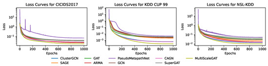
Figure 3.
Training loss curves for PseudoMetapathNet and baseline GNN models on the CICIDS2017, KDD CUP 99, and NSL-KDD datasets. The loss (y-axis) is plotted on a logarithmic scale against the number of training epochs (x-axis), illustrating the convergence behavior of each model.
In conclusion, our framework’s remarkable performance stems from synergistically combining a powerful spectral feature extractor with a novel, semantically aware propagation mechanism that directly addresses the limitations of existing GNNs.
We acknowledge that the performance gap on the original intrusion detection datasets could be further substantiated. To more rigorously test the robustness and generalizability of our framework, we carry out a broader evaluation on three widely-recognized benchmark datasets from the related domain of Graph Anomaly Detection (GAD): Amazon, T-Finance, and Questions. These datasets are known for their challenging characteristics, such as severe class imbalance and heterophily, making them an ideal testbed to validate the effectiveness of our Pseudo-Metapath mechanism beyond its initial application domain. In these datasets, we following the setting from [65], using three metrics: Area Under the Receiver Operating Characteristic Curve (AUROC) and Area Under the Precision–Recall Curve (AUPRC), calculated by average precision, and the Recall score within top-K predictions (Rec@K). We set K as the number of anomalies within the test set. In all metrics, anomalies are treated as the positive class, with higher scores indicating better model performance.
As shown in Table 5 and Table 6, our framework demonstrates a consistently strong, and often superior, performance against a comprehensive suite of GNN baselines. Specifically, on the Amazon and T-Finance datasets, PseudoMetapathNet achieves state-of-the-art results by securing the top performance across all three evaluation metrics (AUROC, AUPRC, and Rec@K). For instance, on T-Finance, it obtains the highest AUROC of 96.40%, AUPRC of 86.62%, and Rec@K of 81.55%, decisively outperforming all competitors. On the challenging Questions dataset, where performance is highly competitive, our model achieves the highest AUPRC of 18.09%. This result is particularly significant, as AUPRC is a more informative metric than AUROC for evaluating models on severely imbalanced datasets, a key feature of this benchmark. These comprehensive results strongly corroborate our central claim: the dynamic Pseudo-Metapath mechanism is a powerful and generalizable strategy for enhancing node anomaly detection in complex graph structures.
Table 5.
Performance comparison of Graph Neural Network models on three different graph anomaly detection datasets. For each dataset and metric, the highest value is indicated in bold and the second-highest in underline. Since the source code of BWMixup is not publicly available, we report its performance as they claimed in their paper [65].
Table 6.
Performance comparison of various models on a optical failure dataset [66].
5.3. Ablation Study
To verify the individual contributions of the key components within our proposed framework, we conducted a series of ablation experiments on all four datasets. We investigated the impact of two core modules: (1) the Beta-Wavelet spectral filter module, responsible for learning frequency-aware node representations and (2) our novel Pseudo-Metapath propagation module, which dynamically routes supervision signals. We evaluated two variants of our model: one without the spectral module and another without the metapath module. The performance degradation relative to the full model is presented in Figure 4.
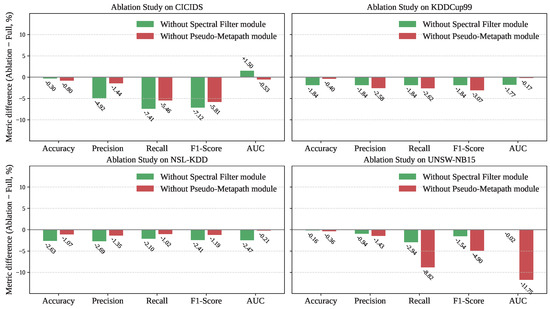
Figure 4.
Ablation analysis on CICIDS, KDDCup99, NSL-KDD, and UNSW-NB15. The bar charts illustrate the performance degradation in Accuracy, Precision, Recall, F1-Score, and AUC when either the Spectral module (green) or the Metapath module (red) is removed from the full model. All values represent the difference (Ablation − Full Model) in percentage (%) relative to the full model’s performance. The zero baseline indicates no change; negative values denote performance decline due to module removal.
The Pseudo-Metapath module, as illustrated by the results, are unequivocally the most critical component of our framework. Removing this module resulted in a substantial and consistent performance drop across all datasets and nearly all metrics. The impact was particularly dramatic on the UNSW-NB15 dataset, where its removal led to a catastrophic decrease in Recall by 8.92% and in AUC by 11.75%. Similarly, on CICIDS, the F1-score plummeted by 7.12%. These significant degradations strongly validate our central hypothesis: standard message passing is insufficient for this task. The dynamic, semantically aware propagation routes learned by the Pseudo-Metapath module are essential for effectively combating the “under-reaching” problem and ensuring that supervision signals reach relevant nodes throughout the network.
The Beta-Wavelet spectral filter also proved to be a vital component for achieving optimal performance. Disabling this module consistently led to a noticeable drop in performance, confirming its role in generating robust initial node embeddings. For instance, on the CICIDS dataset, removing the spectral filter caused a 4.92% drop in Precision. On the NSL-KDD dataset, Accuracy and Precision decreased by 2.53 and 2.09%, respectively. This demonstrates that effectively capturing the high-frequency signals characteristic of network anomalies provides a strong and necessary foundation for the subsequent propagation and classification steps. The synergy between a powerful feature extractor and an intelligent propagation mechanism is therefore key to the model’s success.
In summary, our ablation studies confirm that both the spectral filter and the Pseudo-Metapath module are integral and synergistic components. The spectral filter provides a robust feature basis by capturing anomaly signatures, while the Pseudo-Metapath module provides an indispensable mechanism for effective, long-range information propagation, with the latter being the primary driver of our model’s superior performance.
5.4. Hyper-Parameter Study
In this section, we conduct a comprehensive study to investigate the impact of two critical hyper-parameters on the performance of our proposed model: the number of Dynamic Metapath Learning Layers (aka, Num Layers) and the pseudo-labeling cutoff threshold (aka, Cutoff).
The number of layers determines the model’s complexity and receptive field, while the cutoff threshold controls the confidence required for assigning pseudo-labels during the training process. The model’s performance is measured using Accuracy and Recall, with the results visualized as 3D surface plots to illustrate the interplay between these two parameters. As illustrated in Figure 5 and Figure 6, we can draw several key insights from the experimental results.
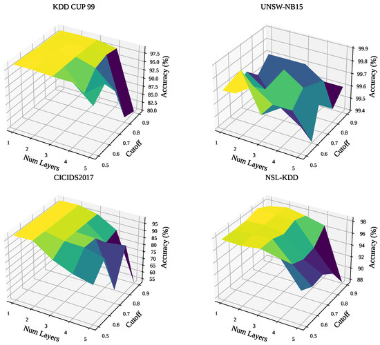
Figure 5.
The impact of varying the number of GNN layers and the cutoff threshold on model Accuracy across the four datasets.
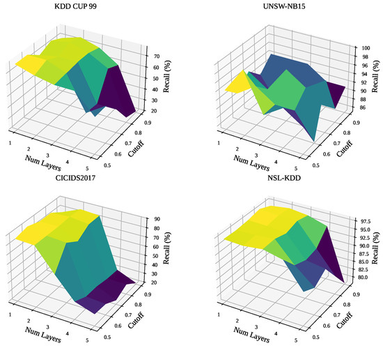
Figure 6.
The impact of varying the number of GNN layers and the cutoff threshold on model Recall across the four datasets.
First, a striking observation is the high degree of consistency between the optimal hyper-parameter regions for maximizing accuracy and recall. Across all datasets, the parameter combinations that yield the highest accuracy also tend to produce the highest recall. This indicates that our model does not require a significant trade-off between these two crucial metrics, simplifying the tuning process.
Second, the Cutoff threshold emerges as the most dominant factor influencing performance. For all four datasets, setting the threshold to a high value (e.g., greater than 0.8) invariably leads to a sharp decline in both accuracy and recall. This is intuitive, as a stricter criterion for classifying positive instances causes the model to miss more potential threats, thereby increasing the number of false negatives and degrading overall performance. The results suggest that a lower-to-mid-range cutoff (approximately 0.5 to 0.7) is optimal.
Third, the ideal model complexity, dictated by the Num Layers, varies depending on the characteristics of the dataset. For KDD CUP 99 and its subset NSL-KDD, a simpler model with two to three layers achieves the best results. Increasing the model’s depth beyond this point leads to a performance drop, likely due to over-smoothing or overfitting. Conversely, for the CICIDS2017 dataset, the model’s performance is largely insensitive to the number of layers, provided that the cutoff threshold is set appropriately. This suggests that the features in this dataset are robust enough to be effectively captured by models of varying depths. The UNSW-NB15 dataset shows a more complex relationship, but a model with 2 layers still provides a reliable and high-performing baseline.
In summary, this study underscores the importance of careful hyper-parameter tuning. The primary guideline for our model is to maintain the Cutoff threshold within a moderate range of [0.5, 0.7]. Within this range, the PseudoMetapathNet with 2 to 3 layers offers a robust and effective configuration for achieving high accuracy and recall across diverse network intrusion detection environments.
5.5. Case Study
To provide a qualitative and intuitive understanding of how PseudoMetapathNet overcomes the limitations of standard GNNs, we conduct a detailed case study on a representative subgraph extracted from the dataset. As illustrated in Figure 7, we selected a homophilous cluster consisting of four interconnected anomaly nodes. This scenario is particularly insightful as it tests a model’s ability to recognize and amplify signals within a group of coordinated malicious entities, a situation where simpler models can surprisingly fail.
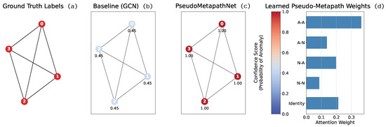
Figure 7.
A case study on a homophilous subgraph with four anomaly nodes. From left to right: (a) The ground truth labels, where all nodes are anomalies (red). (b) The prediction confidence from the baseline GCN, which catastrophically fails by classifying all anomalies as normal (blue). (c) The prediction confidence from our PseudoMetapathNet, which correctly identifies all nodes with maximum confidence (red). (d) The learned attention weights of PseudoMetapathNet for different Pseudo-Metapaths, revealing the high importance assigned to the A-A (Anomaly–Anomaly) path.
The results of the case study clearly demonstrate the superiority of our proposed framework. The leftmost panel of Figure 7 shows the ground truth, a cluster where all four nodes are anomalies. The second panel reveals the surprising failure of the baseline Graph Convolutional Network (GCN) model [67]. Despite the absence of any normal nodes to cause confusion, the GCN misclassifies every single anomaly as normal, yielding a low confidence score of 0.45 for each. This suggests that the standard message-passing mechanism is insufficient for creating a signal reinforcement loop among anomalous peers and may be biased by the globally prevalent normal class.
In stark contrast, the third panel shows the decisive success of our PseudoMetapathNet. It correctly identifies all four nodes as anomalies with the highest possible confidence score of 1.00. The key to this success is revealed in the rightmost panel, which visualizes the learned attention weights. Our model has learned to assign the highest importance to the A-A (Anomaly-Anomaly) metapath, with a weight significantly greater than other path types.
This learned knowledge is critical. When processing this subgraph, PseudoMetapathNet’s dynamic typing and attention mechanism explicitly amplify the information flow along these high-weight A-A paths. This creates a powerful positive feedback loop where each anomaly node mutually reinforces its neighbors’ anomalous status, rapidly driving the prediction confidence to its maximum. This case provides strong qualitative evidence that the Pseudo-Metapath mechanism is crucial for identifying not only isolated threats in heterophilous environments but also coordinated patterns of malicious activity by learning and exploiting the underlying semantic graph structure.
6. Conclusions
In this paper, we propose PseudoMetapathNet, a novel GNN framework that tackles the “under-reaching” problem in optical network intrusion detection by learning dynamic, semantically aware propagation routes—Pseudo-Metapaths. Leveraging Beta-Wavelet spectral filters for high-frequency anomaly capture and a dynamic heterogenization module that assigns transient node types via pseudo-labels, our model guides supervision signals along adaptive, meaningful paths beyond fixed topology. Experiments on four benchmarks show remarkable performance over ML and GNN baselines, with ablations confirming the critical role of Pseudo-Metapath propagation.
Limitations & Future Work
A primary limitation, common to research in this area, is the reliance on general-purpose network intrusion benchmarks due to the scarcity of large-scale, public datasets specific to the physical or control layers of optical networks. While our experiments on these proxies effectively demonstrate our method’s ability to handle the core structural challenges of label sparsity and heterophily, a crucial avenue for future work is to validate PseudoMetapathNet on multiple large-scale real-world optical network traffic data as it becomes accessible, which would confirm its practical utility in the target domain. From a technical perspective, future research should explore scalable spectral approximations to improve efficiency. Second, the model’s performance shows sensitivity to the fixed pseudo-labeling cutoff threshold. A promising future direction is to develop an adaptive thresholding mechanism that can adjust dynamically based on model confidence. Finally, the core concept of learning dynamic propagation routes is highly generalizable. We plan to extend the Pseudo-Metapaths framework to other challenging, label-scarce, and heterophilic domains such as financial fraud detection and online misinformation tracking.
Author Contributions
Conceptualization, G.Q. and H.J.; Methodology, G.Q. and L.Z.; Software, M.G. and X.W.; Validation, H.J., L.Z. and J.X.; Formal analysis, G.Q., M.G. and J.X.; Investigation, H.L. and J.X.; Resources, G.Q.; Data curation, X.W. and H.L.; Writing—original draft, H.L.; Writing—review and editing, H.J., L.Z., H.L. and J.X.; Visualization, X.W. and H.L.; Supervision, G.Q.; Project administration, G.Q. and J.X.; Funding acquisition, G.Q. All authors have read and agreed to the published version of the manuscript.
Funding
This work is supported by the science and technology project of State Grid Corporation of China East China Branch “Research on Key Technologies of Security Protection Architecture System for Optical Transmission System” (Project No. 52992424000L).
Data Availability Statement
The original data presented in the study are openly available in Kaggle.com at https://www.kaggle.com/datasets/hassan06/nslkdd (accessed on 1 September 2025), https://www.kaggle.com/datasets/mrwellsdavid/unsw-nb15 (accessed on 1 September 2025), https://www.kaggle.com/datasets/chethuhn/network-intrusion-dataset (accessed on 1 September 2025), and https://www.kaggle.com/datasets/galaxyh/kdd-cup-1999-data (accessed on 1 September 2025). The GAD dataset, including Amazon, T-Finance, Questions are openly available in https://github.com/squareRoot3/GADBench (accessed on 1 September 2025). The Optical Failure Dataset is openly available in https://github.com/Network-And-Services/optical-failure-dataset (accessed on 1 September 2025).
Conflicts of Interest
Authors Gang Qu, Haochun Jin, Liang Zhang, Minhui Ge and Xin Wu were employed by the State Grid Corporation of China East China Branch. The remaining authors declare that the research was conducted in the absence of any commercial or financial relationships that could be construed as a potential conflict of interest.
References
- Wang, D.; Wang, Y.; Jiang, X.; Zhang, Y.; Pang, Y.; Zhang, M. When large language models meet optical networks: Paving the way for automation. Electronics 2024, 13, 2529. [Google Scholar] [CrossRef]
- Al-Tarawneh, L.; Alqatawneh, A.; Tahat, A.; Saraereh, O. Evolution of optical networks: From legacy networks to next-generation networks. J. Opt. Commun. 2024, 44, s955–s970. [Google Scholar] [CrossRef]
- Agrawal, G.P. Fiber-Optic Communication Systems, 4th ed.; Wiley: Hoboken, NJ, USA, 2012. [Google Scholar]
- O’Mahony, M.J.; Politi, C.; Klonidis, D.; Nejabati, R.; Simeonidou, D. Future optical networks. J. Light. Technol. 2006, 24, 4684–4696. [Google Scholar] [CrossRef]
- Wang, Z.; Raj, A.; Huang, Y.K.; Ip, E.; Borraccini, G.; D’Amico, A.; Han, S.; Qi, Z.; Zussman, G.; Asahi, K.; et al. Toward Intelligent and Efficient Optical Networks: Performance Modeling, Co-Existence, and Field Trials. In Proceedings of the 2025 30th OptoElectronics and Communications Conference (OECC) and 2025 International Conference on Photonics in Switching and Computing (PSC), Sapporo, Japan, 29 June–3 July 2025; IEEE: Piscataway, NJ, USA, 2025; pp. 1–4. [Google Scholar]
- Saleh, B.E.A.; Teich, M.C. Fundamentals of Photonics, 2nd ed.; Wiley: Hoboken, NJ, USA, 2007. [Google Scholar]
- Essiambre, R.J.; Tkach, R.W. Capacity trends and limits of optical communication networks. Proc. IEEE 2012, 100, 1035–1055. [Google Scholar] [CrossRef]
- Mukherjee, B. Optical WDM Networks; Springer: Berlin/Heidelberg, Germany, 2006. [Google Scholar]
- Mohsan, S.A.H.; Mazinani, A.; Sadiq, H.B.; Amjad, H. A survey of optical wireless technologies: Practical considerations, impairments, security issues and future research directions. Opt. Quantum Electron. 2022, 54, 187. [Google Scholar] [CrossRef]
- Skorin-Kapov, N.; Furdek, M.; Zsigmond, S.; Wosinska, L. Physical-layer security in evolving optical networks. IEEE Commun. Mag. 2016, 54, 110–117. [Google Scholar] [CrossRef]
- Kartalopoulos, S.V. Optical network security: Countermeasures in view of attacks. In Optics and Photonics for Counterterrorism and Crime Fighting II; SPIE: Bellingham, WA, USA, 2006; Volume 6402, pp. 49–55. [Google Scholar]
- Wu, Z.; Pan, S.; Chen, F.; Long, G.; Zhang, C.; Yu, P.S. A Comprehensive Survey on Graph Neural Networks. IEEE Trans. Neural Netw. Learn. Syst. 2020, 32, 4–24. [Google Scholar] [CrossRef]
- Akoglu, L.; Tong, H.; Koutra, D. Graph-based Anomaly Detection and Description: A Survey. Data Min. Knowl. Discov. 2015, 29, 626–688. [Google Scholar] [CrossRef]
- Fu, T.; Zhang, J.; Sun, R.; Huang, Y.; Xu, W.; Yang, S.; Zhu, Z.; Chen, H. Optical neural networks: Progress and challenges. Light. Sci. Appl. 2024, 13, 263. [Google Scholar] [CrossRef]
- Li, J.; Zhang, Q.; Liu, W.; Chan, A.B.; Fu, Y.G. Another perspective of over-smoothing: Alleviating semantic over-smoothing in deep GNNs. IEEE Trans. Neural Netw. Learn. Syst. 2024, 36, 6897–6910. [Google Scholar] [CrossRef]
- Li, Q.; Han, Z.; Wu, X. Deeper Insights into Graph Convolutional Networks for Semi-Supervised Learning. In Proceedings of the Thirty-Second AAAI Conference on Artificial Intelligence (AAAI-18), New Orleans, LA, USA, 2–7 February 2018. [Google Scholar]
- Alon, U.; Yahav, E. On the Bottleneck of Graph Neural Networks and its Practical Implications. arXiv 2021, arXiv:2006.05205. [Google Scholar] [CrossRef]
- Topping, J.; Giovanni, F.D.; Chamberlain, B.P.; Dong, X.; Bronstein, M.M. Understanding Over-Squashing and Bottlenecks on Graphs. arXiv 2022, arXiv:2111.14522. [Google Scholar] [CrossRef]
- Peng, J.; Lei, R.; Wei, Z. Beyond over-smoothing: Uncovering the trainability challenges in deep graph neural networks. In Proceedings of the 33rd ACM International Conference on Information and Knowledge Management, Boise, ID, USA, 21–25 October 2024; pp. 1878–1887. [Google Scholar]
- Zheng, Y.; Luan, S.; Chen, L. What is missing for graph homophily? disentangling graph homophily for graph neural networks. Adv. Neural Inf. Process. Syst. 2024, 37, 68406–68452. [Google Scholar]
- Rey, S.; Navarro, M.; Tenorio, V.M.; Segarra, S.; Marques, A.G. Redesigning graph filter-based GNNs to relax the homophily assumption. In Proceedings of the ICASSP 2025-2025 IEEE International Conference on Acoustics, Speech and Signal Processing (ICASSP), Hyderabad, India, 6–11 April 2025; IEEE: Piscataway, NJ, USA, 2025; pp. 1–5. [Google Scholar]
- Zhu, Q.; Han, B.; Zhu, J.; Wen, Y.; Pei, J. Beyond Homophily in Graph Neural Networks: Current Limitations and Effective Designs. In Advances in Neural Information Processing Systems (NeurIPS); Curran Associates, Inc.: Red Hook, NY, USA, 2020. [Google Scholar]
- Pei, H.; Wei, B.; Chang, K.C.; Lei, Y.; Yang, B. Geom-GCN: Geometric Graph Convolutional Networks. arXiv 2020, arXiv:2002.05287. [Google Scholar] [CrossRef]
- Shuman, D.I.; Narang, S.K.; Frossard, P.; Ortega, A.; Vandergheynst, P. The Emerging Field of Signal Processing on Graphs: Extending High-Dimensional Data Analysis to Networks and Other Irregular Domains. IEEE Signal Process. Mag. 2013, 30, 83–98. [Google Scholar] [CrossRef]
- Huang, Q.; Yin, H.; Cui, B.; Cui, Z.; Zhang, Z.; Wang, H.; Wang, E.; Zhou, X. Combining Label Propagation and Simple Models Out-performs Graph Neural Networks. arXiv 2020, arXiv:2010.13993. [Google Scholar] [CrossRef]
- Zhou, D.; Bousquet, O.; Lal, T.N.; Weston, J.; Schölkopf, B. Learning with Local and Global Consistency. In Advances in Neural Information Processing Systems (NIPS); Curran Associates, Inc.: Red Hook, NY, USA, 2004; pp. 321–328. [Google Scholar]
- Li, M.; Jia, L.; Su, X. Global-local graph attention with cyclic pseudo-labels for bitcoin anti-money laundering detection. Sci. Rep. 2025, 15, 22668. [Google Scholar] [CrossRef] [PubMed]
- Yang, S.; Liao, Z.; Chen, R.; Lai, Y.; Xu, W. Multi-view fair-augmentation contrastive graph clustering with reliable pseudo-labels. Inf. Sci. 2024, 674, 120739. [Google Scholar] [CrossRef]
- Lee, D.H. Pseudo-Label: The Simple and Efficient Semi-Supervised Learning Method for Deep Neural Networks. In Proceedings of the ICML 2013 Workshop on Challenges in Representation Learning, Atlanta, GA, USA, 21 June 2013. [Google Scholar]
- Sohn, K.; Berthelot, D.; Carlini, N.; Zhang, Z.; Zhang, H.; Raffel, C.; Cubuk, E.D.; Kurakin, A. FixMatch: Simplifying Semi-Supervised Learning with Consistency and Confidence. In Advances in Neural Information Processing Systems (NeurIPS); Curran Associates, Inc.: Red Hook, NY, USA, 2020. [Google Scholar]
- Qiao, H.; Tong, H.; An, B.; King, I.; Aggarwal, C.; Pang, G. Deep graph anomaly detection: A survey and new perspectives. IEEE Trans. Knowl. Data Eng. 2025, 37, 5106–5126. [Google Scholar] [CrossRef]
- Tu, B.; Yang, X.; He, B.; Chen, Y.; Li, J.; Plaza, A. Anomaly detection in hyperspectral images using adaptive graph frequency location. IEEE Trans. Neural Netw. Learn. Syst. 2024, 36, 12565–12579. [Google Scholar] [CrossRef]
- Zhang, C.; Song, D.; Huang, C.; Swami, A.; Chawla, N.V. Heterogeneous Graph Neural Network. In Proceedings of the KDD’19: Proceedings of the 25th ACM SIGKDD International Conference on Knowledge Discovery & Data Mining, Anchorage, AK, USA, 4–8 August 2019. [Google Scholar]
- Fu, T.; Chen, W.; Sun, Y. MAGNN: Metapath Aggregated Graph Neural Network for Heterogeneous Graph Embedding. In Proceedings of the Web Conference (WWW), Taipei, Taiwan, 20–24 April 2020; pp. 2331–2341. [Google Scholar] [CrossRef]
- Guo, R.; Zou, M.; Zhang, S.; Zhang, X.; Yu, Z.; Feng, Z. Graph Local Homophily Network for Anomaly Detection. In Proceedings of the 33rd ACM International Conference on Information and Knowledge Management, Boise, ID, USA, 21–25 October 2024; pp. 706–716. [Google Scholar]
- Hammond, D.K.; Vandergheynst, P.; Gribonval, R. Wavelets on Graphs via Spectral Graph Theory. Appl. Comput. Harmon. Anal. 2011, 30, 129–150. [Google Scholar] [CrossRef]
- Ruhan, A.; Shen, D.; Liu, L.; Yin, J.; Lin, R. Hyperspectral anomaly detection based on a beta wavelet graph neural network. IEEE MultiMedia 2024, 31, 69–79. [Google Scholar] [CrossRef]
- Tang, J.; Li, J.; Gao, Z.; Li, J. Rethinking graph neural networks for anomaly detection. In Proceedings of the 39th International Conference on Machine Learning, PMLR, Baltimore, MD, USA, 17–23 July 2022; pp. 21076–21089. [Google Scholar]
- Chai, Z.; You, S.; Yang, Y.; Pu, S.; Xu, J.; Cai, H.; Jiang, W. Can abnormality be detected by graph neural networks? In Proceedings of the Thirty-First International Joint Conference on Artificial Intelligence (IJCAI-22), Vienna, Austria, 23–29 July 2022; pp. 1945–1951. [Google Scholar]
- He, M.; Wei, Z.; Xu, H. Bernnet: Learning arbitrary graph spectral filters via bernstein approximation. Adv. Neural Inf. Process. Syst. 2021, 34, 14239–14251. [Google Scholar]
- Shen, D.; Qin, C.; Zhang, Q.; Zhu, H.; Xiong, H. Handling over-smoothing and over-squashing in graph convolution with maximization operation. IEEE Trans. Neural Netw. Learn. Syst. 2024, 36, 8743–8756. [Google Scholar] [CrossRef]
- Jamadandi, A.; Rubio-Madrigal, C.; Burkholz, R. Spectral graph pruning against over-squashing and over-smoothing. Adv. Neural Inf. Process. Syst. 2024, 37, 10348–10379. [Google Scholar]
- Huang, K.; Wang, Y.G.; Li, M. How universal polynomial bases enhance spectral graph neural networks: Heterophily, over-smoothing, and over-squashing. arXiv 2024, arXiv:2405.12474. [Google Scholar] [CrossRef]
- Bing, R.; Yuan, G.; Zhu, M.; Meng, F.; Ma, H.; Qiao, S. Heterogeneous graph neural networks analysis: A survey of techniques, evaluations and applications. Artif. Intell. Rev. 2023, 56, 8003–8042. [Google Scholar] [CrossRef]
- Sang, L.; Wang, Y.; Zhang, Y.; Wu, X. Denoising heterogeneous graph pre-training framework for recommendation. ACM Trans. Inf. Syst. 2025, 43, 1–31. [Google Scholar] [CrossRef]
- Ding, L.; Li, C.; Jin, D.; Ding, S. Survey of spectral clustering based on graph theory. Pattern Recognit. 2024, 151, 110366. [Google Scholar] [CrossRef]
- Wan, G.; Tian, Y.; Huang, W.; Chawla, N.V.; Ye, M. S3GCL: Spectral, swift, spatial graph contrastive learning. In Proceedings of the 41st International Conference on Machine Learning, Vienna, Austria, 21–27 July 2024. [Google Scholar]
- Chung, F.R. Spectral Graph Theory; American Mathematical Society: Providence, RI, USA, 1997; Volume 92. [Google Scholar]
- Luan, S.; Hua, C.; Lu, Q.; Zhu, J.; Zhao, M.; Zhang, S.; Chang, X.W.; Precup, D. Revisiting heterophily for graph neural networks. Adv. Neural Inf. Process. Syst. 2022, 35, 1362–1375. [Google Scholar]
- Maurya, S.K.; Liu, X.; Murata, T. Simplifying approach to node classification in graph neural networks. J. Comput. Sci. 2022, 62, 101695. [Google Scholar] [CrossRef]
- Yun, S.; Jeong, M.; Kim, R.; Kang, J.; Kim, H.J. Graph Transformer Networks. In Advances in Neural Information Processing Systems; Curran Associates, Inc.: Red Hook, NY, USA, 2019. [Google Scholar]
- Caville, E.; Lo, W.W.; Layeghy, S.; Portmann, M. Anomal-E: A self-supervised network intrusion detection system based on graph neural networks. Knowl.-Based Syst. 2022, 258, 110030. [Google Scholar] [CrossRef]
- Biau, G.; Scornet, E. A random forest guided tour. Test 2016, 25, 197–227. [Google Scholar] [CrossRef]
- Xue, H.; Yang, Q.; Chen, S. SVM: Support vector machines. In The Top Ten Algorithms in Data Mining; Chapman and Hall/CRC: Boca Raton, FL, USA, 2009; pp. 51–74. [Google Scholar]
- Windeatt, T. Accuracy/diversity and ensemble MLP classifier design. IEEE Trans. Neural Netw. 2006, 17, 1194–1211. [Google Scholar] [CrossRef] [PubMed]
- Natekin, A.; Knoll, A. Gradient boosting machines, a tutorial. Front. Neurorobot. 2013, 7, 21. [Google Scholar] [CrossRef] [PubMed]
- Chen, T.; Guestrin, C. XGBoost: A scalable tree boosting system. In Proceedings of the ACM SIGKDD International Conference on Knowledge Discovery and Data Mining (KDD ’16), San Francisco, CA, USA, 13–17 August 2016; Association for Computing Machinery: New York, NY, USA, 2016; pp. 785–794. [Google Scholar]
- Quinlan, J.R. Learning decision tree classifiers. ACM Comput. Surv. (CSUR) 1996, 28, 71–72. [Google Scholar] [CrossRef]
- LaValley, M.P. Logistic regression. Circulation 2008, 117, 2395–2399. [Google Scholar] [CrossRef]
- Kim, D.; Oh, A. How to Find Your Friendly Neighborhood: Graph Attention Design with Self-Supervision. arXiv 2022, arXiv:2204.04879. [Google Scholar] [CrossRef]
- Hamilton, W.L.; Ying, R.; Leskovec, J. Inductive Representation Learning on Large Graphs. In Advances in Neural Information Processing Systems; Curran Associates, Inc.: Red Hook, NY, USA, 2017; pp. 1024–1034. [Google Scholar]
- Bianchi, F.M.; Grattarola, D.; Livi, L.; Alippi, C. Graph neural networks with convolutional arma filters. IEEE Trans. Pattern Anal. Mach. Intell. 2021, 44, 3496–3507. [Google Scholar] [CrossRef]
- Hu, W.; Liu, B.; Gomes, J.; Zitnik, M.; Liang, P.; Pande, V.; Leskovec, J. Strategies for Pre-training Graph Neural Networks. arXiv 2019, arXiv:1905.12265. [Google Scholar]
- Bo, D.; Wang, X.; Shi, C.; Shen, H. Beyond low-frequency information in graph convolutional networks. In Proceedings of the AAAI Conference on Artificial Intelligence, Palo Alto, CA, USA, 2–9 February 2021; Volume 35, pp. 3950–3957. [Google Scholar]
- Do, T.U.; Ta, V.C. Tackling under-reaching issue in Beta-Wavelet filters with mixup augmentation for graph anomaly detection. Expert Syst. Appl. 2025, 275, 127033. [Google Scholar] [CrossRef]
- Silva, M.F.; Pacini, A.; Sgambelluri, A.; Valcarenghi, L. Learning long- and short-term temporal patterns for ML-driven fault management in optical communication networks. IEEE Trans. Netw. Serv. Manag. 2022, 19, 2195–2206. [Google Scholar] [CrossRef]
- Kipf, T.N.; Welling, M. Semi-Supervised Classification with Graph Convolutional Networks. arXiv 2016, arXiv:1609.02907. [Google Scholar]
Disclaimer/Publisher’s Note: The statements, opinions and data contained in all publications are solely those of the individual author(s) and contributor(s) and not of MDPI and/or the editor(s). MDPI and/or the editor(s) disclaim responsibility for any injury to people or property resulting from any ideas, methods, instructions or products referred to in the content. |
© 2025 by the authors. Licensee MDPI, Basel, Switzerland. This article is an open access article distributed under the terms and conditions of the Creative Commons Attribution (CC BY) license (https://creativecommons.org/licenses/by/4.0/).