Article

Spectral Collocation Method for Solving Nonlinear Riesz Distributed-Order Fractional Differential Equations

by
Ammar Lachin
1,
Mohammed A. Abdelkawy
2 and
Saratha Sathasivam
1,*
1
School of Mathematical Sciences, Universiti Sains Malaysia, Penang 11800 USM, Malaysia
2
Department of Mathematics and Statistics, Faculty of Science, Imam Mohammad Ibn Saud Islamic University (IMSIU), Riyadh 11623, Saudi Arabia
*
Author to whom correspondence should be addressed.
Mathematics 2025, 13(21), 3425; https://doi.org/10.3390/math13213425
Submission received: 26 September 2025 / Revised: 18 October 2025 / Accepted: 22 October 2025 / Published: 27 October 2025
(This article belongs to the Section E: Applied Mathematics)

Abstract

In this article, we present an efficient and highly accurate numerical scheme that achieves exponential convergence for solving nonlinear Riesz distributed-order fractional differential equations (RDFDEs) in one- and two-dimensional initial–boundary value problems. The proposed method is based on a two-stage collocation framework. In the first stage, spatial discretization is performed using the shifted Legendre–Gauss–Lobatto (SL-G-L) collocation method, where the approximate solutions and spatial derivatives are expressed in terms of shifted Legendre polynomial expansions. This reduces the original problem to a system of fractional differential equations (FDEs) for the expansion coefficients. Then, the temporal discretization is achieved in the second stage via Romanovski–Gauss–Radau collocation approach, which converts the system into a system of algebraic equations that can be solved efficiently. The method is applied to one- and two-dimensional nonlinear RDFDEs, and numerical experiments confirm its spectral accuracy, computational efficiency, and reliability. Existing numerical approaches to distributed-order fractional models often suffer from poor accuracy, instability in nonlinear settings, and high computational costs. By combining the efficiency of Legendre polynomials for bounded spatial domains with the stability of Romanovski polynomials for temporal discretization, the proposed two-stage framework effectively overcomes these limitations and achieves superior accuracy and stability.

1. Introduction

Fractional calculus has evolved into an effective mathematical framework for modeling physical [1], biological [2], and engineering systems [3] characterized by memory effects [4], anomalous diffusion [5], and long-range interactions. Unlike classical models based on integer-order derivatives, fractional differential equations incorporate nonlocal operators that enable more accurate and flexible descriptions of complex dynamic phenomena. The foundations of fractional calculus were laid by early mathematicians such as Leibniz, Riemann, and Liouville, and were significantly extended by Caputo [6] in a form that became direct applicable in modeling physical processes. In recent decades, FDEs have been broadly applied to describe sub-diffusive transport in porous media [7], and viscoelastic behavior in complex materials [8], among many other phenomena.
A significant extension of traditional FDEs is the class of distributed-order fractional differential equations (DOFDEs), in which the derivative order is distributed over a continuous range rather than being a fixed value. This allows for the modeling of systems where the degree of memory or diffusion is not uniform but varies across time or space [9]. Time-DOFDEs are commonly used to model ultra-slow diffusion and complex viscoelastic responses for which traditional single-order models are insufficient. Space-distributed-order FDEs, on the other hand, are useful for capturing spatial heterogeneity in anomalous transport and diffusion [10].
When nonlinearities are introduced, fractional partial differential equations (FPDEs)—especially those including the Riesz fractional operator—become even more powerful in describing real-world processes [11] such as anomalous heat transfer, nonlinear wave propagation, and reaction-diffusion systems in biological and physical media [12]. However, the presence of both nonlocality and nonlinearity makes these equations analytically intractable in most cases, necessitating robust numerical solutions.
The present study introduces a novel spectral collocation framework that combines Legendre and Romanovski polynomials to solve nonlinear RDFDEs. This hybrid formulation represents a new methodological contribution, enabling exponential convergence, high numerical accuracy, and efficient computation with only a few terms in the approximate solution. The proposed approach effectively addresses the long-standing challenges of handling both nonlocality and nonlinearity while maintaining stability and computational efficiency in one- and two-dimensional problems. The principal contributions of this work include the development of this new collocation strategy, a thorough validation through benchmark examples, and a detailed complexity analysis confirming its computational advantages.
The remainder of this paper is organized as follows. Section 2 reviews related studies and discusses the motivation, challenges, and problem context of the nonlinear RDFDEs. Section 3 introduces the necessary preliminaries and theoretical foundations. In Section 4, we present the proposed spectral collocation method based on the combined use of Romanovski and Legendre polynomials, including its one-dimensional formulation, two-dimensional extension, and reduction to a system of time-ordinary differential equations. Section 5 provides comprehensive numerical experiments that demonstrate the accuracy and efficiency of the proposed approach, including a detailed computational complexity analysis. Finally, Section 6 summarizes the main conclusions and emphasizes the overall effectiveness and significance of the proposed method.

2. Related Work and Problem Statement

Various numerical approaches have been developed to address the challenges mentioned in the previous section. Wang and Cai [13] proposed a finite difference method to solve nonlinear time–space DOFDEs, where an implicit difference scheme was used to achieve convergence in both time and space. Khan et al. [14] developed a higher-order implicit finite difference iterative approach to solve the two-dimensional time fractional Cable equation. Fei and Huang [15] introduced a Galerkin spectral method using Legendre polynomials for distributed order time-fractional fourth-order PDE. Luo et al. [16] developed a robust and accurate second-order ADI Galerkin technique to solve the three-dimensional nonlocal heat model. A spectral Tau method was used in [17] to find a solution of a family of FDEs. To solve nonlinear time-fractional Burgers’ equations, Hadhoud et al. [18] used a collocation approach with non-polynomial B-spline method and obtained highly accurate results. M. A. Abdelkawy et al. [19] used a spectral collocation technique to solve the nonlinear DOFDE of Bagley–Torvik numerically, validating the spectral accuracy of their approach. They demonstrated the method’s efficacy in resolving both fractional dynamics and nonlinear effects. In [20] a unified spectral Galerkin-collocation technique was utilized to handle high-order singular boundary value problems, yielding highly accurate approximations. More recently, Lachin et al. [21] proposed an efficient collocation method for solving Riesz distributed FDEs. Their approach employs a two-step spectral strategy: spatial discretization is handled using SL-G-L collocation method, while temporal discretization uses a Romanovski–Gauss–Radau collocation technique. This technique simplifies the original problem into a set of algebraic equations, offering exponential convergence and high spectral accuracy in both one- and two-dimensional settings, as confirmed through numerical examples.
Despite these developments, several limitations persist in existing numerical methods for distributed-order FPDEs. Many techniques are tailored to either time- or space-distributed formulations, but few address the fully coupled time–space distributed-order models, particularly in the nonlinear case. Most current schemes are designed for linear or weakly nonlinear equations and struggle when extended to problems with strong nonlinearities or spatial heterogeneity. Furthermore, commonly used methods such as low-order finite differences and basic Galerkin schemes often suffer from low accuracy near boundaries, inefficient handling of singularities, and high computational costs for fine-scale resolution. Many approaches also assume uniform fractional order distributions, which limits their ability to model realistic systems with space- or time-dependent distribution densities. Additionally, theoretical guarantees like convergence and stability are often lacking, especially for nonlinear multidimensional problems.
Spectral methods have shown promise in overcoming these issues due to their high-order accuracy and global approximation properties. Spectral methods approximate the solution using global orthogonal polynomials, leading to exponential convergence for a smooth solution [22]. In the fractional calculus context, these methods are well-suited for handling the nonlocal nature of fractional operators. Adaptive collocation strategies have further enhanced their applicability by refining the approximation near singularities and localized features. Legendre, Jacobi, and Chebyshev polynomials [23] are among the most commonly used bases due to their orthogonality and numerical stability, while Romanovski polynomials offer additional flexibility in capturing solution behavior over unbounded or singular domains [21]. When applied to nonlinear distributed-order problems, these polynomial-based spectral schemes not only improve accuracy but also reduce computational cost, making them effective tools for modeling complex systems in various scientific fields.
Nonlinear Riesz distributed-order FPDEs pose significant challenges due to the simultaneous presence of nonlocal operators and nonlinear terms, which often leads to high computational costs and limited accuracy in existing schemes. In this work, we address these limitations by developing a spectral collocation method that combines Legendre and Romanovski polynomials in a two-stage framework. The proposed approach achieves exponential convergence while substantially reducing computational cost, and it is capable of efficiently handling both one- and two-dimensional problems. The method has the remarkable advantage of producing highly accurate results with only a limited number of terms in the approximate solution, further highlighting its efficiency. Numerical experiments on benchmark RDFDEs confirm the method’s spectral accuracy, stability, and efficiency, with clear improvements over existing approaches. By advancing the numerical treatment of this challenging class of equations, our work contributes both a novel methodology and practical evidence of its effectiveness, thereby enhancing the modeling and simulation of memory-driven, heterogeneous, and nonlinear systems.

3. Preliminaries and Theories

This section presents the essential mathematical concepts and tools that form the basis of the proposed numerical method. We begin with a review of key definitions and properties from fractional calculus, with particular emphasis on the Riesz fractional derivative, which plays a central role in modeling anomalous diffusion and nonlocal dynamics. Additionally, we introduce the Romanovski polynomials, highlighting their analytical properties and associated quadrature rules. These foundational elements collectively provide the theoretical framework for constructing an accurate and efficient spectral collocation method for solving nonlinear RDFDEs.
Definition 1.
For ν > 0 , the Riemann–Liouville fractional integral is defined [24] as
J ν G ( ξ ) = 1 Γ ( ν ) 0 ξ ( ξ ψ ) ( ν 1 ) G ( ψ ) d ψ , ν > 0 , ξ > 0 , J 0 G ( ξ ) = G ( ξ ) ,
where Γ is the Gamma function
Γ ( ν ) = 0 ξ ν 1 e ξ d ξ .
Some of the integral J ν properties are
J θ J ν G ( ξ ) = J θ + ν G ( ξ ) , J θ J ν G ( ξ ) = J ν J θ G ( ξ ) , J ν ξ θ = Γ ( θ + 1 ) Γ ( ν + θ + 1 ) ξ ν + θ .
Definition 2.
Ref. [24] defines Caputo fractional derivative for ν > 0 as
D ν G ( ξ ) = 1 Γ ( r ν ) 0 ξ ( ξ ψ ) r ν 1 d r d ψ r G ( ψ ) d ψ , r 1 < ν r , ξ > 0 .
Some of the fractional differential operator D ν properties:
J ν D ν G ( ξ ) = G ( ξ ) j = 0 r 1 G ( j ) ( 0 + ) ξ j j !
D ν ξ θ = 0 for θ N 0 and θ < ν , Γ ( θ + 1 ) Γ ( θ ν + 1 ) ξ θ ν for θ N 0 and θ ν or θ > ν or θ N ,
where the floor and ceiling functions are ν and ν respectively, N 0 = { 0 , 1 , 2 , } , and N = { 1 , 2 , 3 , } .
Definition 3.
Refs. [25,26] define Riesz fractional derivative for a function G ( ξ , η ) and ν > 0 as
ν G ( ξ , η ) | ξ | ν = 1 2 c o s ( ν π 2 ) ( D L ν ξ G ( ξ , η ) + D R ν ξ G ( ξ , η ) ) ,
where D L ν ξ G ( ξ , η ) and D R ν ξ G ( ξ , η ) represent the Riemann–Liouville fractional derivative (R-LFD) for the first spatial variable ξ with m 1 < ν < m , are given as
D L ν ξ G ( ξ , η ) = 1 Γ ( m ν ) m ξ m a ( η ) ξ ( ξ χ ) ( m ν 1 ) G ( χ , η ) d χ , D R ν ξ G ( ξ , η ) = ( 1 ) m Γ ( m ν ) m ξ m ξ b ( η ) ( χ ξ ) ( m ν 1 ) G ( χ , η ) d χ ,
and the fractional derivative operators for the second space variable η can be similarly defined and denoted by D L ν η G ( ξ , η ) , D R ν η G ( ξ , η ) .
Legendre polynomials L i ( ξ ) , i N are defined on [ 1 , 1 ] and satisfy Rodrigues formula
L i ( ξ ) = ( 1 ) i 2 i i ! D i ( ( 1 ξ 2 ) i ) .
These polynomials can be obtained by the recursive relation
L 0 ( ξ ) = 1 , L 1 ( ξ ) = ξ , L i + 2 ( ξ ) = 2 i + 3 i + 2 x L i + 1 ( ξ ) k + 1 k + 2 L i ( ξ ) .
The nth derivative of Legendre polynomials can be expressed as a summation of these polynomials
L i ( m ) ( ξ ) = j = 0 ( i + j = e v e n ) i m C m ( i , j ) L j ( ξ ) ,
where
C m ( i , j ) = 2 m 1 ( 2 j + 1 ) Γ ( m + i j 2 ) Γ ( m + i + j + 1 2 ) Γ ( m ) Γ ( 2 m + i j 2 ) Γ ( 3 m + i + j 2 ) .
Moreover, Legendre polynomials satisfy the orthogonality relation
( L i ( ξ ) , L j ( ξ ) ) = 1 1 L i ( ξ ) L j ( ξ ) w ( ξ ) = h i δ i j ,
where w ( ξ ) = 1 , h i = 2 2 i + 1 .
The Legendre–Gauss–Lobatto quadratures are the zeros of the derivative of Legendre polynomial ξ L N ( ξ ) can be written as
ξ N , 0 = 1 , ξ N , N = 1 , ξ N , i ( i = 1 , 2 , , N 1 ) ,
and the corresponding Christoffel numbers (quadrature wights) are
ϖ N , i = 2 N ( N + 1 ) ( L N ( ξ N , i ) ) 2 .
Those nodes and weights can be used to convert the previous integrals into summations as follows:
1 1 ϕ ( ξ ) d ξ = i = 0 N ϖ N , i ϕ ( ξ N , i ) , ϕ S 2 N 1 [ 1 , 1 ] ,
where S 2 N 1 [ 1 , 1 ] is the set of all polynomials with degrees less than or equal 2 N 1 . Those quadratures also can be used to write the discrete inner product on [ 1 , 1 ] in the form of a summation as
( ϕ , ψ ) w = i = 0 N ϕ ( ξ N , i ) ψ ( ξ N , i ) ϖ N , i .
Similarly, Legendre Gauss Radau quadratures ξ N , i ( i = 0 , 1 , , N ) are the zeros of L N ( ξ ) + L N + 1 ( ξ ) , their corresponding Christoffel numbers are ϖ N , 0 = 2 ( N + 1 ) 2 , ϖ N , i = 1 ξ i ( N + 1 ) 2 ( L N ( ξ i ) ) 2 .
The shifted Legendre polynomials can be used for the purpose of using the interval [ 0 , 1 ] in the models under study. They can be obtained by using the transformation ξ = 2 ξ L 1 on Legendre polynomials. For simplicity we will denote them as L L , j ( ξ ) = L j ( 2 ξ L 1 ) . Additionally, those polynomials have the analytical form
L L , j ( ξ ) = l = 0 j ( 1 ) j + l ( j + l ) ! ( j l ) ! ( l ! ) 2 L l ξ l ,
and satisfy the recursive formula
( j + 1 ) L L , j + 1 ( ξ ) = ( 2 j + 1 ) ( 2 ξ L 1 ) L L , j ( ξ ) j L L , j 1 ( ξ ) , j = 1 , 2 ,
and the orthogonality condition
0 L L L , i ( ξ ) L L , l ( ξ ) w L ( ξ ) d ξ = l L δ i l ,
where w L ( ξ ) = 1 and l L = L 2 l + 1 .
The shifted Legendre polynomials can be used to express a square integrable function G ( ξ ) on the interval [ 0 , L ] as
G ( ξ ) = k = 0 a k L L , k ( ξ ) ,
where the coefficients ak are
a k = 1 k L 0 L G ( ξ ) L L , k ( ξ ) w k ( ξ ) d ξ , k N 0 .
In approximations, usually, only the first N + 1 terms of the polynomial are taken. So a function G ( ξ ) can be written as an expansion using shifted Legendre polynomials as
G N ( ξ ) k = 0 N a k L L , k ( ξ ) .
Definition 4.
Romanovski polynomials of degree i and type ( α , β ) are denoted by R i ( α , β ) , and defined as [27]
R i ( α , β ) : = ( α + 1 ) i i ! 2 F 1 ( i , α + β + i + 1 ; α + 1 , t ) .
The following formula produces ( N + 1 ) one dimensional Romanovski-Jacobi polynomials (RJPs), denoted by R i ( α , β ) ( t ) , with α > 1 and β < 2 N α 1 , defined on [ 0 , )
R i ( α , β ) ( t ) = k = 0 i ( 1 ) k Γ ( α β i ) Γ ( α + i + 1 ) Γ ( α + k + 1 ) Γ ( α β i k ) Γ ( i k + 1 ) k ! t k , i = 0 , , N .
RJPs are orthogonal on [ 0 , ) with the weight function W ( t ) = t α ( 1 + t ) β , and satisfy the orthogonality condition
0 R n ( α , β ) ( x ) R m ( α , β ) ( x ) w ( x ) d x = h n δ n m .
Here, δ n m denotes the Kronecker delta function, and h i = Γ ( i + α + 1 ) Γ ( i α β ) Γ ( 2 i + α + β + 1 ) i ! Γ ( i β ) is the normalization constant.
Theorem 1.
For α > 1 , 0 i , m N 2 and α + β + N + 1 < 0 ,
0 R i ( α , β ) ( t ) R m ( α , β ) ( t ) w α , β ( t ) d t = ( 1 ) i + 1 Γ ( i α β ) Γ ( i + α + 1 ) ( β + 1 ) i i ! ( 2 i + α + β + 1 ) Γ ( β ) δ i m ,
where w α , β ( t ) = t α ( 1 + t ) β is the weight function [27].
The formula
R i ( α , β ) ( t ) = J i ( α , β ) ( 1 + 2 t )
shows the relationship between Romanovski polynomials R i ( α , β ) ( t ) and Jacobi polynomials J i ( α , β ) ( t ) . The explicit form of Romanovski polynomials is
R i ( α , β ) ( t ) : = m = 0 i a i , m ( α , β ) t m , a i , m ( α , β ) = α + β + m + i m α + i m + i .
Lemma 1
([28]). RJPs can be obtained by the recursive formula
R i + 1 ( α , β ) ( t ) = R i ( α , β ) ( t ) A i ( α , β ) ( t ) B i ( α , β ) C i ( α , β ) R i 1 ( α , β ) ( t ) , i 1 , R 0 ( α , β ) ( t ) , R 1 ( α , β ) ( t ) = 1 + α + t ( α + β + 2 ) ,
where
A i ( α , β ) = ( β + α + 2 i + 1 ) ( β + α + 2 i + 2 ) ( β + α + i + 1 ) ( i + 1 ) , B i ( α , β ) = ( β + α + 2 i + 1 ) ( ( β + α ) ( α + 2 i + 1 ) + 2 i ( i + 1 ) ) ( β + α + i + 1 ) ( β + α + 2 i ) ( i + 1 ) , C i ( α , β ) = ( β + α + 2 i + 2 ) ( α + i ) ( β + i ) ( β + α + 2 i ) ( β + α + i + 1 ) ( i + 1 ) .
Lemma 2.
For the eigenvalues δ i α , β = i ( i + α + β + 1 ) < 0 of Sturm–Liouville’s singluar problem, RJPs are the eigenfunctions
S α , β R i α , β ( t ) = δ i α , β R i α , β ( t ) .
Theorem 2
([28]). For
A i α , β = ( i + α ) ( i + β ) ( i + α + β + 1 ) ( 2 i + α + β + 1 ) ( 2 i + α + β ) , B i α , β = ( β α ) ( β + α + i + 1 ) i ( β + α + 2 i ) ( β + α + 2 i + 2 ) , C i α , β = i ( i + 1 ) ( β + α + i + 1 ) ( β + α + 2 i + 1 ) ( β + α + 2 i + 2 ) ,
Romanovski–Jacobi polynomials saticfy
t ( t + 1 ) t R i α , β ( t ) = A i α , β R i 1 α , β ( t ) + B i α , β R i α , β ( t ) + C i α , β R i + 1 α , β ( t ) .
Theorem 3
([29]). The derivatives of RJPs are
d r d t r R m α , β ( t ) = l = 0 m r C l , m α , β , r R l α , β ( t ) ,
where
C l , m α , β , r = ( 1 ) r Γ ( m α β ) Γ ( m α β r ) c k n r ( r + α , r + β , α , β ) ,
and
c k n r ( r + α , r + β , α , β ) = Γ ( m + α + 1 ) Γ ( m α β r ) ( β + α + 2 k + 1 ) Γ ( α + k + 1 ) Γ ( α β k ) × n = 0 m + r k ( 1 ) ( n + 1 ) Γ ( 2 k n β α + 1 ) Γ ( n + k + α + 1 ) Γ ( n m k r β α ) Γ ( m n k r + 1 ) Γ ( n + k + r + α + 1 ) n ! .
Theorem 4
([29]). Denoted by t i i = 0 M , the Romanovski–Jacobi-Gauss nodes are the zeros of R M + 1 α , β . The corresponding weights are
ϖ i α , β = G M α , β R M α , β ( t i ) t R M + 1 α , β ( t i ) = G ˜ M α , β t i ( 1 + t i ) t R M + 1 α , β ( t i ) 2 ,
where
G M α , β = ( α + β + 2 M + 2 ) Γ ( α β M 1 ) Γ ( α + M + 1 ) Γ ( β M ) ( M + 1 ) ! , G ˜ M α , β = Γ ( α β M 1 ) Γ ( α + M + 2 ) Γ ( β M 1 ) ( M + 1 ) ! .

4. Proposed Spectral Collocation Method

4.1. One-Dimensional Formulation

In this subsection, we will solve numerically the nonlinear initial–boundary value problem presented below over the region Ω = ( a , b ) :
u t = 1 2 Q 1 ( ν 1 ) ν 1 u | x | ν 1 d ν 1 + 0 1 Q 2 ( ν 2 ) ν 2 u | x | ν 2 d ν 2 + f ( u , x , t ) , where , x Ω , t 0 ,
with ν 1 ( 1 , 2 ) and ν 2 ( 0 , 1 ) representing the fractional derivative’s order, and
u ( a , t ) = ϕ 1 ( t ) , u ( b , t ) = ϕ 2 ( t ) , u ( x , 0 ) = χ ( x ) , x Ω .
In this method, we aim to simplify the nonlinear coupled system (8) and (9) into a system of FDEs. To achieve this, we will be using the Legendre–Gauss–Lobatto quadrature nodes over the interval ( a , b ) , which guarantees that the boundary conditions are satisfied without any need of using additional equations. Thus, this approach improves the numerical solutions accuracy. Additionally, we will approximate the solution u ( x , t ) using a finite series of shifted Legendre polynomials L L , i ( x )
u ( x , t ) = i = 0 N c i ( t ) L L , i ( x ) .
The coefficients (2) and the orthogonality condition (1) allows us to write
c i ( t ) = 1 i L 0 L w L ( x ) L L , i ( x ) u ( x , t ) d x .
To estimate the previous integral, we will use the SL-G-L quadrature formula. For all ψ S 2 N 1 [ 0 , L ] ,
0 L w ( x ) ψ ( x ) d x = i = 0 N ϖ N , i L ψ ( x N , i L ) ,
where we represent the nodes as x N , i L ( i = 0 , 1 , , N ) and the corresponding Christoffel numbers of SL-G-L quadrature formula over [ 0 , L ] by ϖ N , i L ( i = 0 , 1 , , N ) .
Moreover, the property (12) allows us to write the coefficients c i as a finite summation as follows:
c i ( t ) = 1 i L j = 0 N L i ( x N , j L ) ( ϖ N , j L ) u ( x N , j L , t ) ,
which allows the approximate solution to have the form
u ( x , t ) = i , j = 0 N ϖ N , j L i L L L , i ( x ) L L , i ( x N , j L ) u ( x N , j L , t ) .
Riesz fractional derivative ν u ( x , t ) | x | ν can be presented as
ν u ( x , t ) | x | ν = 1 2 c o s ( ν π 2 ) ( D L ν x u ( x , t ) + D R ν x u ( x , t ) ) ,
where D L ν x u ( x , t ) and D R ν x u ( x , t ) are left and right R-LFD for x respectively, given as
D L ν x u ( x , t ) = 1 Γ ( 1 ν ) x 0 x ( x χ ) ν u ( χ , t ) d χ = i , j = 0 N ϖ N , j L i L D L ν x L L , i ( x ) L L , i ( x N , j L ) u ( x N , j L , t ) ,
D R ν x u ( x , t ) = 1 Γ ( 1 ν ) x x 1 ( χ x ) ν u ( χ , t ) d χ = i , j = 0 N ϖ N , j L i L D R ν x L L , i ( x ) L L , i ( x N , j L ) u ( x N , j L , t ) .
From the previous series of steps we can write
ν u ( x , t ) | x | ν = 1 2 c o s ( ν π 2 ) i , j = 0 N ϖ N , j L i L L L , i ( x N , j L ) D L ν x L L , i ( x ) + D R ν x L L , i ( x ) u ( x N , j L , t ) = i , j = 0 N ϖ N , j L i L L L , i ( x N , j L ) B i ν ( x ) u ( x N , j L , t ) .
where B i ν ( x ) = 1 2 c o s ( ν π 2 ) D L ν x L L , i ( x ) + D R ν x L L , i ( x ) , see [23], and
D L ν x L L , i ( x ) = Γ ( i + 1 ) x ν Γ ( i ν + 1 ) J i ( ν , ν ) 2 x L 1 , D R ν x L L , i ( x ) = Γ ( i + 1 ) ( L x ) ν Γ ( i ν + 1 ) J i ( ν , ν ) 2 x L 1 ,
such that J i ( ν , ν ) represents Jacobi polynomials.
For the time derivative in (14),
u ( x , t ) t = i , j = 0 N ϖ N , j L i L L L , i ( x ) L L , i ( x N , j L ) d u L , N ( t ) d t ,
by denoting u ( x N , j L , t ) as u L , N ( t ) and substituting in (8), one can write
i , j = 0 N ϖ N , j L i L L L , i ( x ) L L , i ( x N , j L ) d u L , N ( t ) d t = 1 2 Q 1 ( ν 1 ) i , j = 0 N ϖ N , j L i L L L , i ( x N , j L ) B i ν 1 ( x ) u L , N ( t ) d ν 1 + 0 1 Q 2 ( ν 2 ) i , j = 0 N ϖ N , j L i L L L , i ( x N , j L ) B i ν 2 ( x ) u L , N ( t ) d ν 2 + f ( u , x , t ) .
Denoting
F 1 ( ν 1 ) = Q 1 ( ν 1 ) i , j = 0 N ϖ N , j L i L L L , i ( x N , j L ) B i ν 1 ( x ) u L , N ( t ) , F 2 ( ν 2 ) = Q 2 ( ν 2 ) i , j = 0 N ϖ N , j L i L L L , i ( x N , j L ) B i ν 2 ( x ) u L , N ( t ) ,
we get
i , j = 0 N ϖ N , j L i L L L , i ( x N , j L ) L L , i ( x ) d u L , N ( t ) d t = 1 2 F 1 ( ν 1 ) d ν 1 + 0 1 F 2 ( ν 2 ) d ν 2 + f ( u , x , t ) .
With the variable change α 1 = ν 1 1 , we can write
i , j = 0 N ϖ N , j L i L L L , i ( x N , j L ) L L , i ( x ) d u L , N ( t ) d t = 0 1 F 1 ( α 1 + 1 ) d α 1 + 0 1 F 2 ( ν 2 ) d ν 2 + f ( u , x , t ) .
We can represent the integral in the previous equation, which is the distributed order fractional term, as a summation using the SL-G-L as follows:
i , j = 0 N ϖ N , j L i L L L , i ( x ) L L , i ( x N , j L ) d u L , N ( t ) d t = s 1 = 0 S 1 ϖ S 1 , s 1 F 1 ( α S 1 , s 1 + 1 ) + s 2 = 0 S 2 ϖ S 2 , s 2 F 2 ( α S 2 , s 2 ) + f ( u , x , t ) .

4.2. Two-Dimensional Extension

This subsection contains an efficient numerical approach to solve the following nonlinear two-dimensional RDFDE:
u t = 1 2 Q 1 ( ν 1 ) ν 1 u | x | ν 1 d ν 1 + 0 1 Q 2 ( ν 2 ) ν 2 u | x | ν 2 d ν 2 + 1 2 P 1 ( θ 1 ) θ 1 u | y | θ 1 d θ 1 + 0 1 P 2 ( θ 2 ) θ 2 u | y | θ 2 d θ 2 + f ( u , x , y , t ) ,
with the boundary and initial conditions
u ( x , y , t ) = 0 f o r ( x , y , t ) Ω × ( 0 , T ] , u ( x , y , 0 ) = ψ ( x , y ) , ( x , y ) Ω ,
and ( x , y ) Ω , t ( 0 , T ] , ν 1 , θ 1 ( 1 , 2 ) , ν 2 , θ 2 ( 0 , 1 ) . The nonnegative weight functions Q 1 ( ν 1 ) , Q 2 ( ν 2 ) , P 1 ( θ 1 ) and P 2 ( θ 2 ) , respectively, satisfy 0 < 1 2 Q 1 ( ν 1 ) d ν 1 < , 0 < 0 1 Q 2 ( ν 2 ) d ν 2 < , 0 < 1 2 P 1 ( θ 1 ) d θ 1 < , and 0 < 0 1 P 2 ( θ 2 ) d θ 2 < .
We will reduce this equation combined with its initial and boundary conditions into a system of FDEs using SL-G-L collocation approach. The resulting system can be easily solved using the known methods in the numerical analysis literature.
We begin our method by writing the approximate solution as
u ( x , y , t ) = j = 0 M i = 0 N c i , j ( t ) L L 1 , i ( x ) L L 2 , j ( y ) .
Besides the orthogonality relation, we will use shifted Legendre polynomials L L 1 , N ( x ) and L L 2 , M ( y ) with the corresponding SL-G-L nodes x N , i L 1 ( i = 0 , 1 , , N ) and y M , j L 2 ( j = 0 , 1 , , M ) respectively, so we will be able to write the coefficients as
c i , j ( t ) = 1 i L 1 j L 2 l = 0 M k = 0 N ϖ N , k L 1 L L 1 , i ( x N , k L 1 ) ϖ M , l L 2 L L 2 , j ( y M , l L 2 ) u ( x N , k L 1 , y M , l L 2 , t ) .
By denoting u k , l ( t ) = u ( x N , k L 1 , y M , l L 2 , t ) , we will be able to write the approximate solution (19) as
u ( x , y , t ) = j , l = 0 M i , k = 0 N ϖ N , k L 1 L L 1 , i ( x N , k L 1 ) ϖ M , l L 2 L L 2 , j ( y M , l L 2 ) i L 1 j L 2 L L 1 , i ( x ) L L 2 , j ( y ) u k , l ( t ) .
Riesz fractional derivative ν u ( x , y , t ) | x | ν can be expressed by using R-LFD as
ν u ( x , y , t ) | x | ν = 1 2 c o s ( ν π 2 ) ( x D L ν u ( x , y , t ) + D R ν x u ( x , y , t ) ) ,
where the left and right R-LFD for the variable x are D L ν x u ( x , y , t ) and D R ν x u ( x , y , t ) respectively, given as follows:
D L ν x u ( x , y , t ) = 1 Γ ( 1 ν ) x 0 x ( x χ ) ν u ( χ , y , t ) d χ = j , l = 0 M i , k = 0 N ϖ N , k L 1 L L 1 , i ( x N , k L 1 ) ϖ M , l L 2 L L 2 , j ( y M , l L 2 ) i L 1 j L 2 D L ν x L L 1 , i ( x ) L L 2 , j ( y ) u k , l ( t ) ,
D R ν x u ( x , y , t ) = 1 Γ ( 1 ν ) x x 1 ( χ x ) ν u ( χ , y , t ) d χ = j , l = 0 M i , k = 0 N ϖ N , k L 1 L L 1 , i ( x N , k L 1 ) ϖ M , l L 2 L L 2 , j ( y M , l L 2 ) i L 1 j L 2 D R ν x L L 1 , i ( x ) L L 2 , j ( y ) u k , l ( t ) .
The previous series of steps allows us to write
ν u ( x , y , t ) | x | ν = j , l = 0 M i , k = 0 N ϖ N , k L 1 L L 1 , i ( x N , k L 1 ) ϖ M , l L 2 L L 2 , j ( y M , l L 2 ) i L 1 j L 2 B i ν ( x ) L L 2 , j ( y ) u k , l ( t ) .
Similarly, the Riesz fractional derivative ν u ( x , y , t ) | y | ν can be expressed as
ν u ( x , y , t ) | y | ν = 1 2 c o s ( ν π 2 ) ( y D L ν u ( x , y , t ) + D R ν y u ( x , y , t ) ) ,
where the left and right R-LFD for the variable y are D L ν y u ( x , y , t ) and D R ν y u ( x , y , t ) respectively, given as follows:
D L ν y u ( x , y , t ) = 1 Γ ( 1 ν ) y 0 y ( y η ) ν u ( x , η , t ) d η = j , l = 0 M i , k = 0 N ϖ N , k L 1 L L 1 , i ( x N , k L 1 ) ϖ M , l L 2 L L 2 , j ( y M , l L 2 ) i L 1 j L 2 L L 1 , i ( x ) D L ν y L L 2 , j ( y ) u k , l ( t ) ,
D R ν y u ( x , y , t ) = 1 Γ ( 1 ν ) y y 1 ( η y ) ν u ( x , η , t ) d η = j , l = 0 M i , k = 0 N ϖ N , k L 1 L L 1 , i ( x N , k L 1 ) ϖ M , l L 2 L L 2 , j ( y M , l L 2 ) i L 1 j L 2 L L 1 , i ( x ) D R ν y L L 2 , j ( y ) u k , l ( t ) .
Accordingly, we can write
ν u ( x , y , t ) | y | ν = j , l = 0 M i , k = 0 N ϖ N , k L 1 L L 1 , i ( x N , k L 1 ) ϖ M , l L 2 L L 2 , j ( y M , l L 2 ) i L 1 j L 2 L L 1 , i ( x ) B j ν ( y ) u k , l ( t ) .
Using (20) for the time fractional derivative, we get
u ( x , y , t ) t = j , l = 0 M i , k = 0 N ϖ N , k L 1 L L 1 , i ( x N , k L 1 ) ϖ M , l L 2 L L 2 , j ( y M , l L 2 ) i L 1 j L 2 L L 1 , i ( x ) L L 2 , j ( y ) d u k , l ( t ) d t .
Substituting in (17) gives us
j , l = 0 M i , k = 0 N ϖ N , k L 1 L L 1 , i ( x N , k L 1 ) ϖ M , l L 2 L L 2 , j ( y M , l L 2 ) i L 1 j L 2 L L 1 , i ( x ) L L 2 , j ( y ) d u k , l ( t ) d t = 1 2 Q 1 ( ν 1 ) j , l = 0 M i , k = 0 N ϖ N , k L 1 L L 1 , i ( x N , k L 1 ) ϖ M , l L 2 L L 2 , j ( y M , l L 2 ) i L 1 j L 2 B i ν 1 ( x ) L L 2 , j ( y ) u k , l ( t ) d ν 1 + 0 1 Q 2 ( ν 2 ) j , l = 0 M i , k = 0 N ϖ N , k L 1 L L 1 , i ( x N , k L 1 ) ϖ M , l L 2 L L 2 , j ( y M , l L 2 ) i L 1 j L 2 B i ν 2 ( x ) L L 2 , j ( y ) u k , l ( t ) d ν 2 + 1 2 P 1 ( θ 1 ) j , l = 0 M i , k = 0 N ϖ N , k L 1 L L 1 , i ( x N , k L 1 ) ϖ M , l L 2 L L 2 , j ( y M , l L 2 ) i L 1 j L 2 L L 1 , i ( x ) B j θ 1 ( y ) u k , l ( t ) d θ 1 + 0 1 P 2 ( θ 2 ) j , l = 0 M i , k = 0 N ϖ N , k L 1 L L 1 , i ( x N , k L 1 ) ϖ M , l L 2 L L 2 , j ( y M , l L 2 ) i L 1 j L 2 L L 1 , i ( x ) B j θ 2 ( y ) u k , l ( t ) d θ 2 + f ( u , x , y , t ) .
Denoting
H 1 ( ν 1 ) = Q 1 ( ν 1 ) j , l = 0 M i , k = 0 N ϖ N , k L 1 L L 1 , i ( x N , k L 1 ) ϖ M , l L 2 L L 2 , j ( y M , l L 2 ) i L 1 j L 2 B i ν 1 ( x ) L L 2 , j ( y ) u k , l ( t ) H 2 ( ν 2 ) = Q 2 ( ν 2 ) j , l = 0 M i , k = 0 N ϖ N , k L 1 L L 1 , i ( x N , k L 1 ) ϖ M , l L 2 L L 2 , j ( y M , l L 2 ) i L 1 j L 2 B i ν 2 ( x ) L L 2 , j ( y ) u k , l ( t ) K 1 ( θ 1 ) = P 1 ( θ 1 ) j , l = 0 M i , k = 0 N ϖ N , k L 1 L L 1 , i ( x N , k L 1 ) ϖ M , l L 2 L L 2 , j ( y M , l L 2 ) i L 1 j L 2 L L 1 , i ( x ) B j θ 1 ( y ) u k , l ( t ) K 2 ( θ 2 ) = P 2 ( θ 2 ) j , l = 0 M i , k = 0 N ϖ N , k L 1 L L 1 , i ( x N , k L 1 ) ϖ M , l L 2 L L 2 , j ( y M , l L 2 ) i L 1 j L 2 L L 1 , i ( x ) B j θ 2 ( y ) u k , l ( t ) ,
we can write
j , l = 0 M i , k = 0 N ϖ N , k L 1 L L 1 , i ( x N , k L 1 ) ϖ M , l L 2 L L 2 , j ( y M , l L 2 ) i L 1 j L 2 L L 1 , i ( x ) L L 2 , j ( y ) d u k , l ( t ) d t = 1 2 H 1 ( ν 1 ) d ν 1 + 0 1 H 2 ( ν 2 ) d ν 2 + 1 2 K 1 ( θ 1 ) d θ 1 + 0 1 K 2 ( θ 2 ) d θ 2 + f ( u , x , y , t ) .
By changing the variables α 1 = ν 1 1 , γ 1 = θ 1 1 , we can write
j , l = 0 M i , k = 0 N ϖ N , k L 1 L L 1 , i ( x N , k L 1 ) ϖ M , l L 2 L L 2 , j ( y M , l L 2 ) i L 1 j L 2 L L 1 , i ( x ) L L 2 , j ( y ) d u k , l ( t ) d t = 0 1 H 1 ( α 1 + 1 ) d α 1 + 0 1 H 2 ( ν 2 ) d ν 2 + 0 1 K 1 ( γ 1 + 1 ) d γ 1 + 0 1 K 2 ( θ 2 ) d θ 2 + f ( u , x , y , t ) .
This equation can be written as
j , l = 0 M i , k = 0 N ϖ N , k L 1 L L 1 , i ( x N , k L 1 ) ϖ M , l L 2 L L 2 , j ( y M , l L 2 ) i L 1 j L 2 L L 1 , i ( x ) L L 2 , j ( y ) d u k , l ( t ) d t = r 1 = 0 R 1 ϖ R 1 , r 1 H 1 ( α 1 R 1 , r 1 + 1 ) + r 2 = 0 R 2 ϖ R 2 , r 2 H 2 ( ν 2 R 2 , r 2 ) + s 1 = 0 S 1 ϖ S 1 , s 1 K 1 ( γ 1 S 1 , s 1 + 1 ) + s 2 = 0 S 2 ϖ S 2 , s 2 K 2 ( θ 2 S 2 , s 2 ) + f ( u , x , y , t ) .

4.3. Reduction to Time-Ordinary Systems

This section introduces a numerical integration method that uses Romanovski polynomials and Gauss–Radau interpolation to solve time-based systems of ordinary differential equations with initial values. We will generalize the systems presented in (16) and (21). Consider
d u r ( t ) d t = G r ( t , u 1 ( t ) , , u R ( t ) ) , t 0 , r = 1 , , R ,
with
u r ( 0 ) = τ r , r = 1 , , R ,
where G r ( t , u 1 ( t ) , , u R ( t ) ) , r = 1 , , R , are given functions.
The approximate solution can be expressed as
u r ( t ) = i = 0 K b r , i R T , i ( t ) , r = 1 , , R ,
and the first derivative will be
d u r ( t ) d t = i = 0 K b r , i d R T , i ( t ) d t , r = 1 , , R .
From (22)–(25), we get
i = 0 K b r , i d R T , i ( t ) d t = G r t , i = 0 K b 1 , i R T , i ( t ) , , i = 0 K b R , i R T , i ( t ) , r = 1 , , R , t 0 ,
i = 0 K b r , i R T , i ( 0 ) = τ r , r = 1 , , R ,
where we set the residual to zero in (22) at R K collocation points, which gives us R K algebraic equations
i = 0 K b r , i d R T , i ( t K , s T ) d t = G r ( t K , s T , i = 0 K b 1 , i R T , i ( t K , s T ) , , i = 0 K b R , i R T , i ( t K , s T ) ) , r = 1 , , R , s = 1 , , K .
Additionally, we will collocate the initial conditions using Gauss Radau interpolation nodes in (23) which will give another R algebraic equations
i = 0 K b r , i R T , i ( t K , 0 T ) = τ r , r = 1 , , R .
Combining the previous algebraic systems gives us a directly solvable system of R ( K + 1 ) algebraic equations. This demonstrates that the approximated solutions (24) can be evaluated.

5. Numerical Experiments and Discussion

This section presents a set of numerical experiments designed to illustrate the robustness and high precision of the proposed collocation method when applied to one- and two-dimensional nonlinear RDFDEs. These results serve to validate the theoretical properties of the algorithm and to illustrate its practical effectiveness. All numerical computations and graphical visualizations were performed using Wolfram Mathematica 13.3 on a standard desktop computer equipped with an Intel Core i7 processor and 8 GB RAM.

5.1. One-Dimensional Test Problem

Example 1.
Let us take the problem
u t = 1 2 Q 1 ( ν 1 ) ν 1 u | x | ν 1 d ν 1 + 0 1 Q 2 ( ν 2 ) ν 2 u | x | ν 2 d ν 2 + f ( u , x , t ) , ( x , t ) [ 0 , 1 ] × [ 0 , T ]
under the listed conditions below:
u ( 1 , t ) = u ( 0 , t ) = 0 ,
u ( x , 0 ) = x 2 ( 1 x ) 2 ,
with
Q 1 ( ν 1 ) = 2 λ 1 cos ( ν 1 π / 2 ) Γ ( 5 ν 1 ) , Q 2 ( ν 2 ) = 2 λ 2 cos ( ν 2 π / 2 ) Γ ( 5 ν 2 ) .
Let f ( u , x , t ) be defined to yield an exact solution of the form
u ( x , t ) = ( e t + r t r ) ( 1 x ) 2 x 2 .
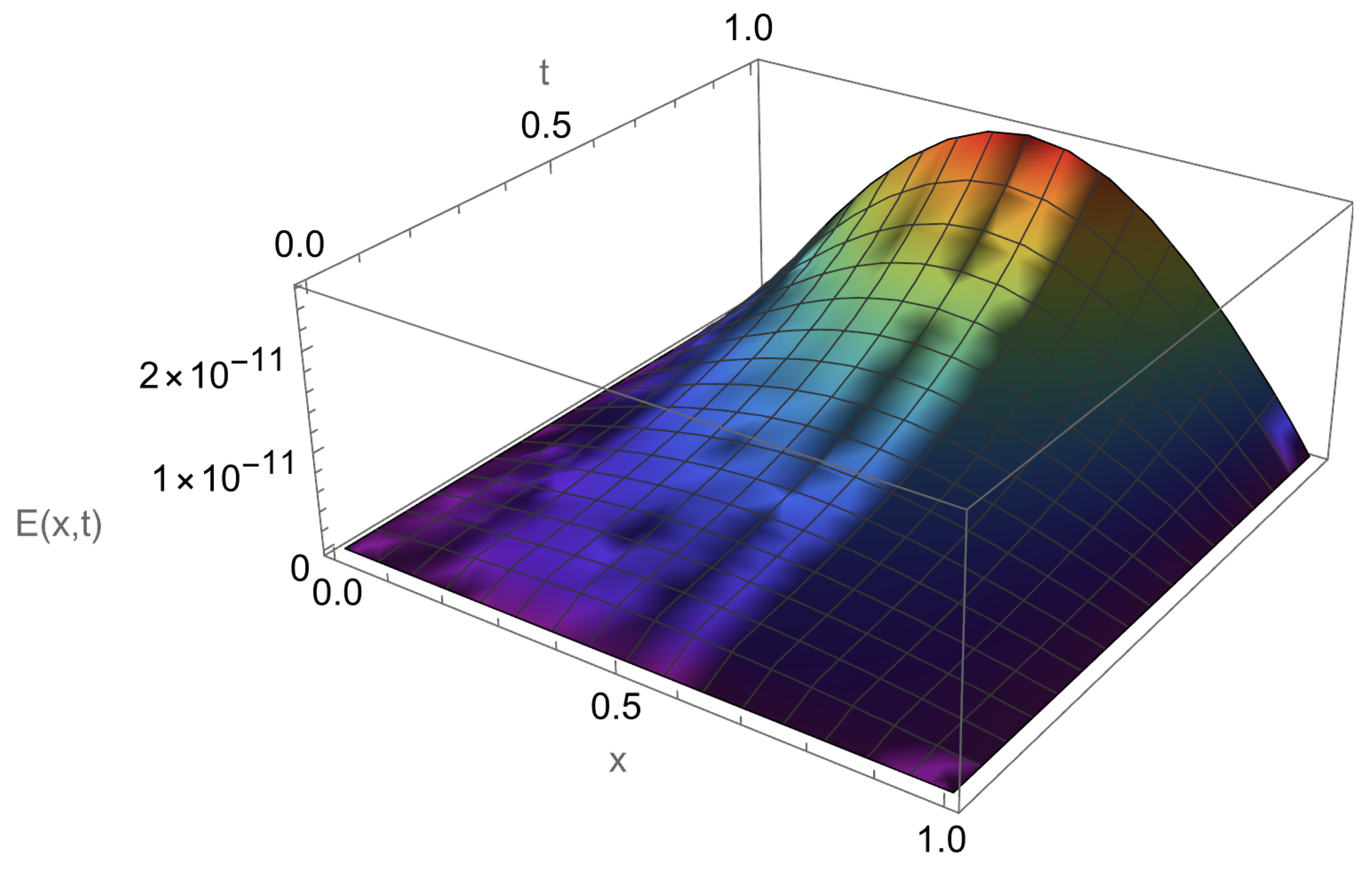
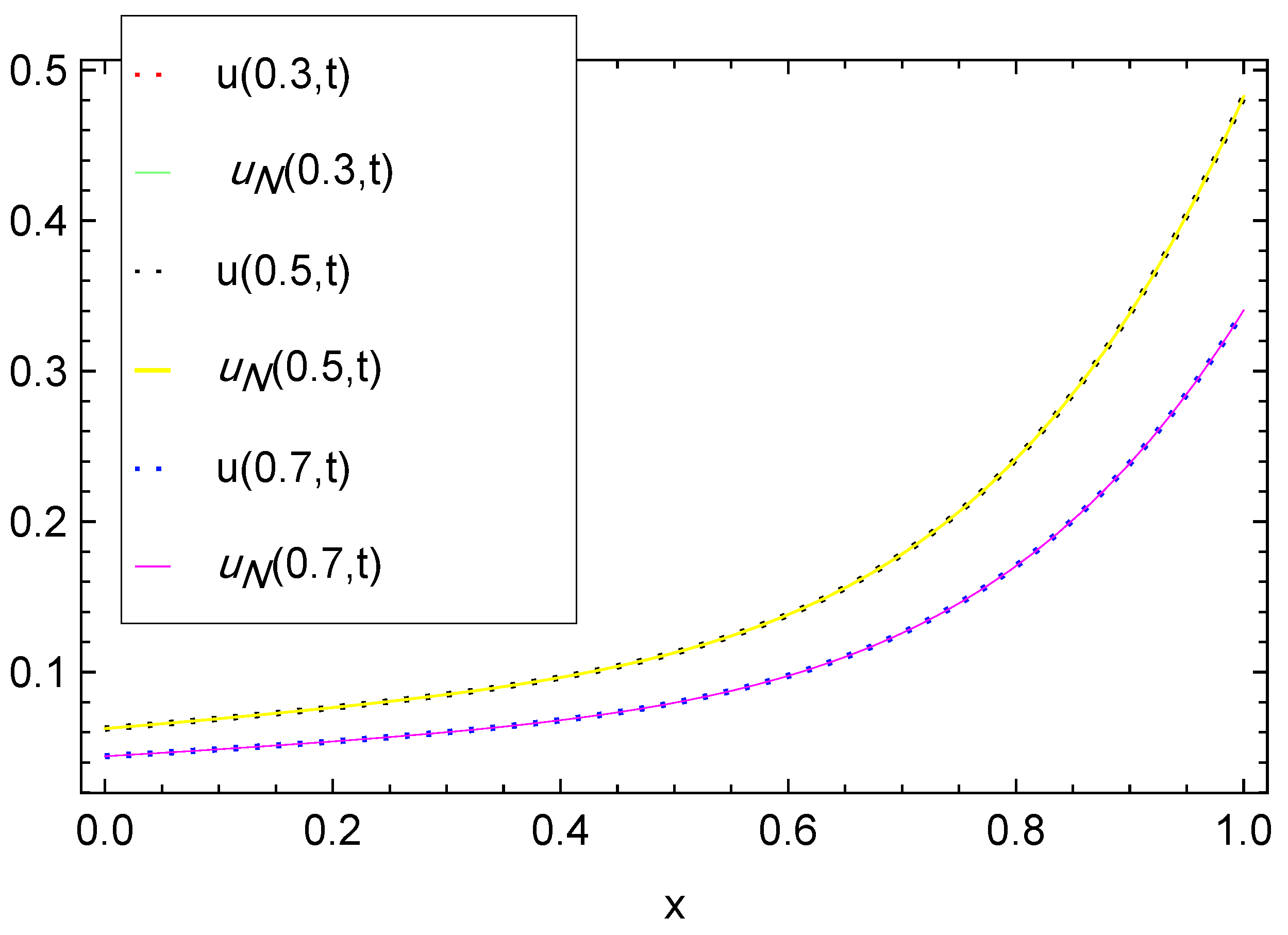
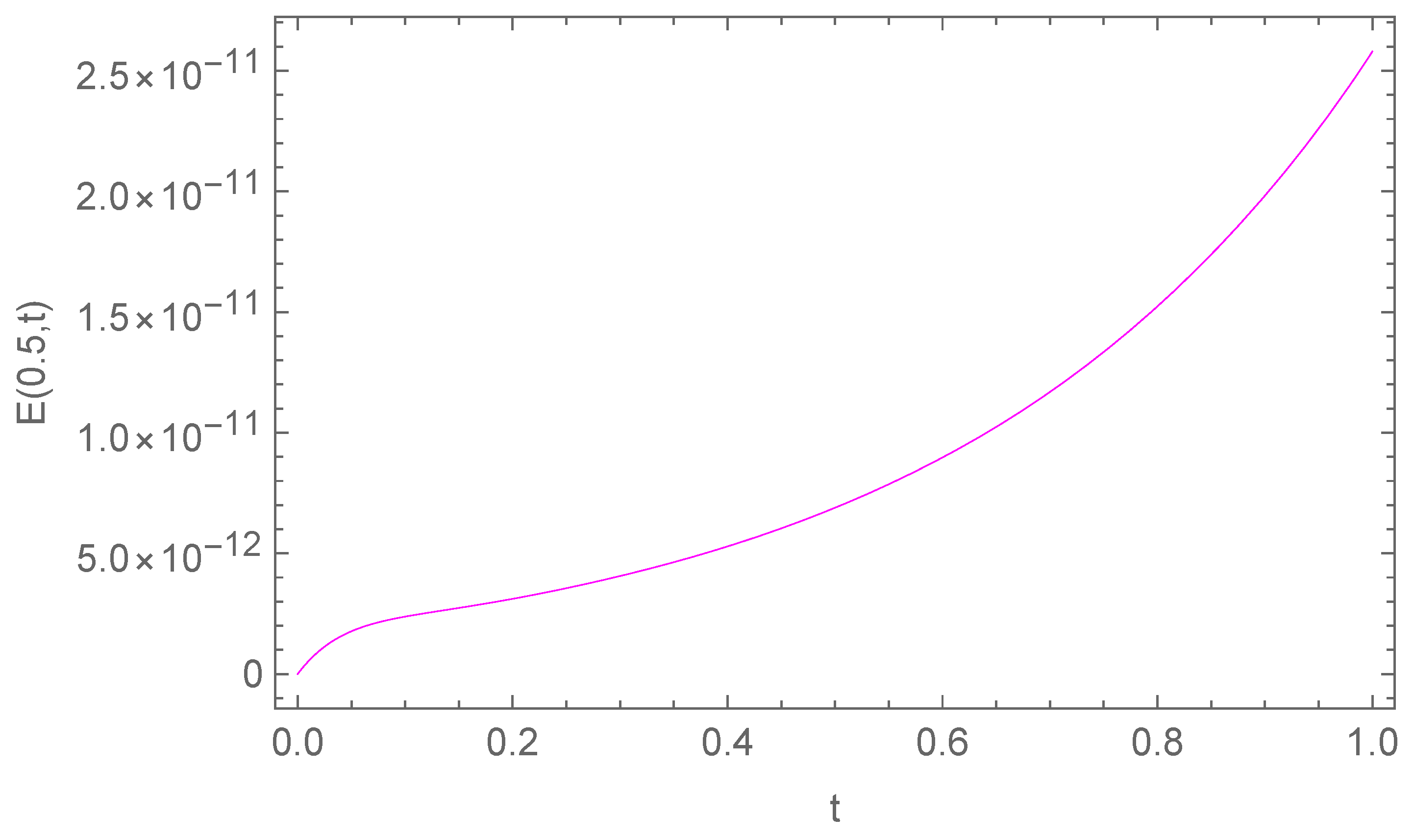
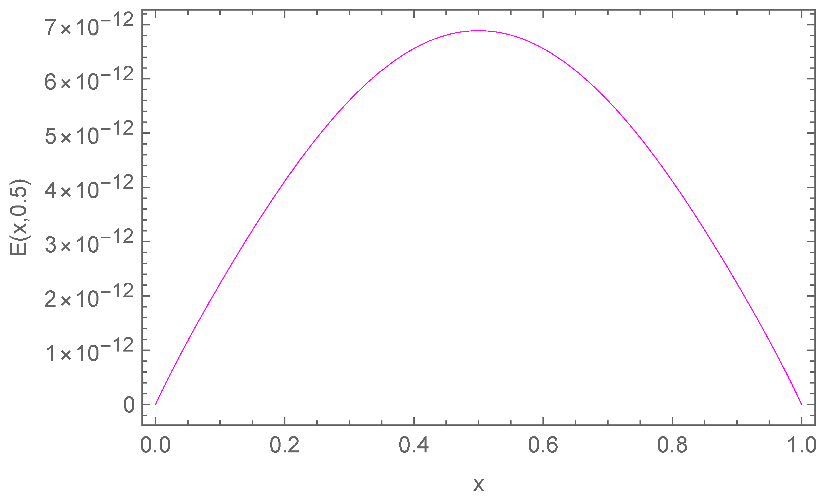
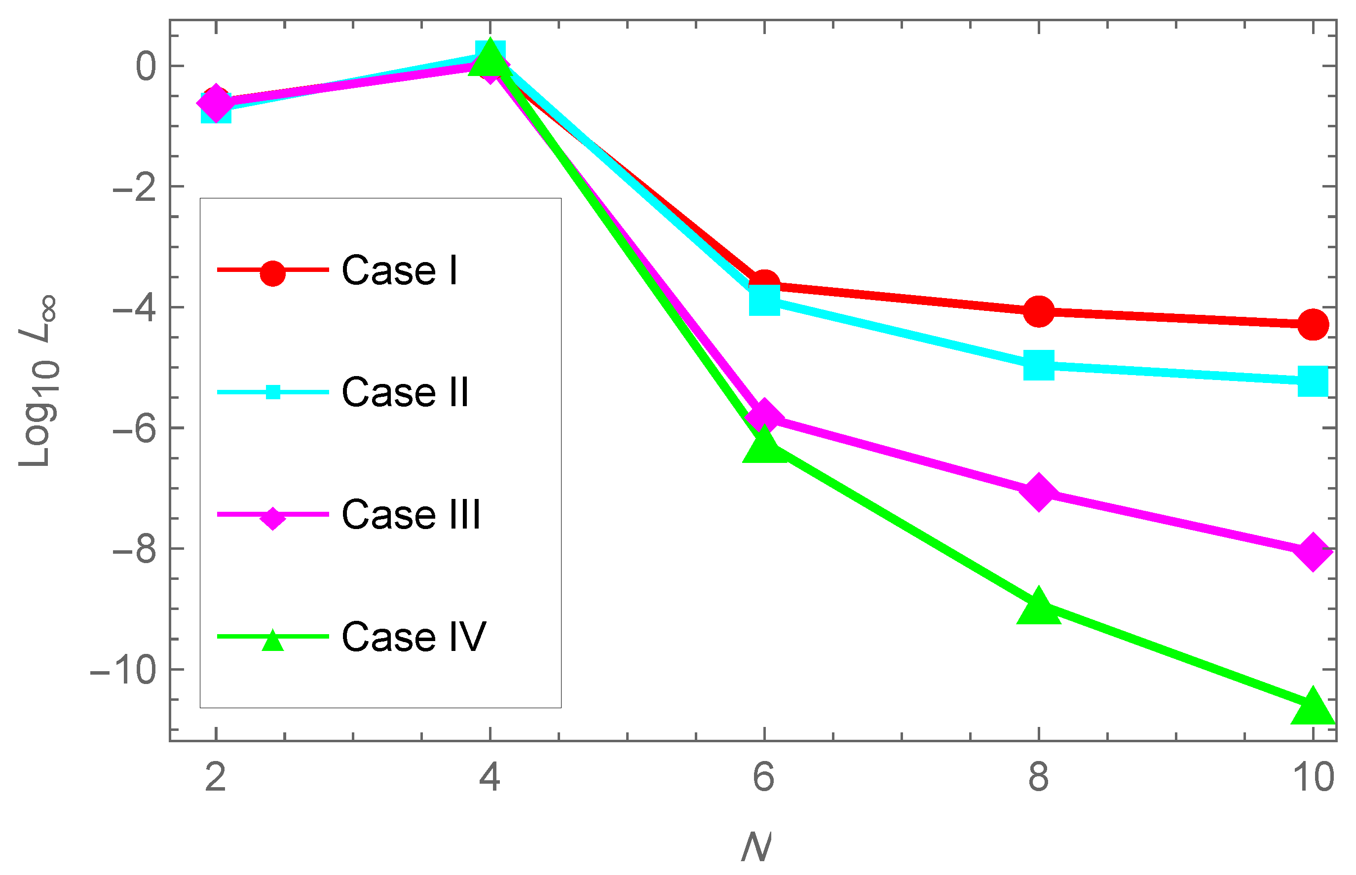
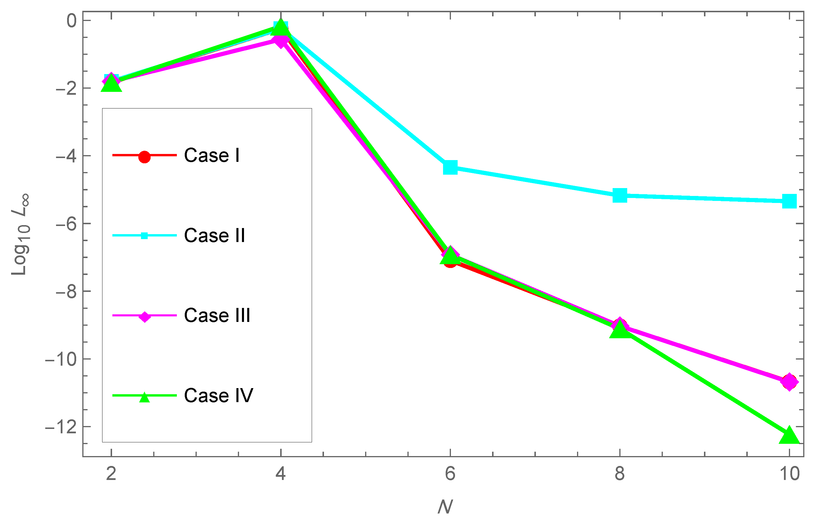
In Table 1, we report the maximum absolute errors generated by applying the proposed algorithm to Example 1. Figure 1 displays the approximate solution u N ( x , t ) for the chosen case N = 10 , α = 5 , β = 60 , λ 0 = 0 , λ 1 = λ 2 = 1 , r = 5 . For selected points within the domain, Figure 2 illustrates the absolute error E ( x , t ) along the x t -plane. Figure 3 and Figure 4 demonstrate excellent agreement between the numerical approximation and the exact solution u ( x , t ) . Figure 5 and Figure 6 show the corresponding absolute errors along the t- and the x-direction, respectively. The convergence decay curve in Figure 7 confirms the exponential and rapid convergence of the proposed method. As the number of collocation points N increases, the error decreases exponentially, which aligns with the smoothness of both the exact solution and the Romanovski–Legendre basis functions. Consistent results across all parameter sets further verify the accuracy and stability of the two-stage spectral collocation formulation for smooth problems.

5.2. Two-Dimensional Test Problem

Example 2.
Consider Equation (17) with Ω = ( 0 , 1 ) × ( 0 , 1 ) ,
Q 1 ( ν 1 ) = 2 λ 1 cos ( ν 1 π / 2 ) Γ ( 5 ν 1 ) , Q 2 ( ν 2 ) = 2 λ 2 cos ( ν 2 π / 2 ) Γ ( 5 ν 2 ) , P 1 ( θ 1 ) = 2 λ 1 cos ( θ 1 π / 2 ) Γ ( 5 θ 1 ) , P 2 ( θ 2 ) = 2 λ 2 cos ( θ 2 π / 2 ) Γ ( 5 θ 2 ) ,
f ( u , x , y , t ) = x 2 y 2 ( 1 x 2 ) ( 1 y 2 ) ( t r 1 r 2 + e t ) λ 0 sin ( t x 2 y 2 ( 1 x 2 ) ( 1 y 2 ) ( t r r + e t ) ) + λ 0 sin ( t u ) e t y 2 ( 1 y ) 2 ( r t r + e t ) [ λ 1 ( W 1 ( 1 x ) + W 1 ( x ) ) + λ 2 ( W 2 ( 1 x ) + W 2 ( x ) ) ] x 2 ( 1 x ) 2 ( r t r + e t ) [ λ 1 ( W 1 ( 1 y ) + W 1 ( y ) ) + λ 2 ( W 2 ( 1 y ) + W 2 ( y ) ) ]
and u 0 ( x , y ) = x 2 y 2 ( 1 x ) 2 ( 1 y ) 2 , where
W 1 ( ρ ) = Γ ( 5 ) ρ 3 ρ 2 ln ( ρ ) 2 Γ ( 4 ) 3 ρ 2 2 ρ ln ( ρ ) ρ 2 ρ ( ln ( ρ ) ) 2 + Γ ( 3 ) 6 ρ 2 ln ( ρ ) 5 ρ 3 ( ln ( ρ ) ) 2 + 2 ρ 2 ( ln ( ρ ) ) 3 , W 2 ( ρ ) = Γ ( 5 ) ρ 4 ρ 3 ln ( ρ ) 2 Γ ( 4 ) 4 ρ 3 3 ρ 2 ln ( ρ ) ρ 3 ρ 2 ( ln ( ρ ) ) 2 + Γ ( 3 ) 12 ρ 2 6 ρ ln ( ρ ) 7 ρ 2 5 ρ ( ln ( ρ ) ) 2 + 2 ρ 2 2 ρ ( ln ( ρ ) ) 3 .
The exact solution has the form u ( x , y , t ) = x 2 y 2 ( 1 x 2 ) ( 1 y 2 ) ( r t r + e t ) .
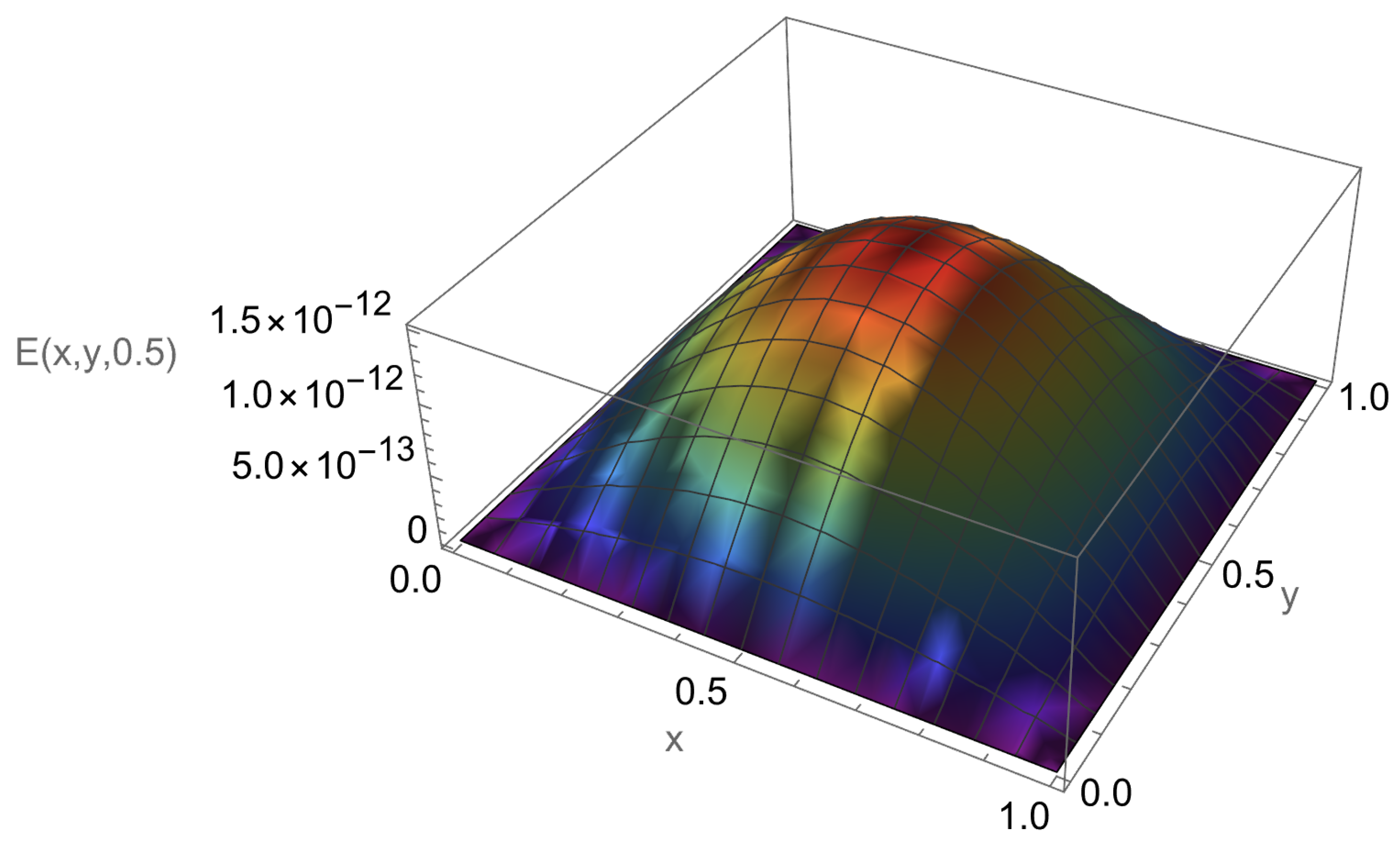
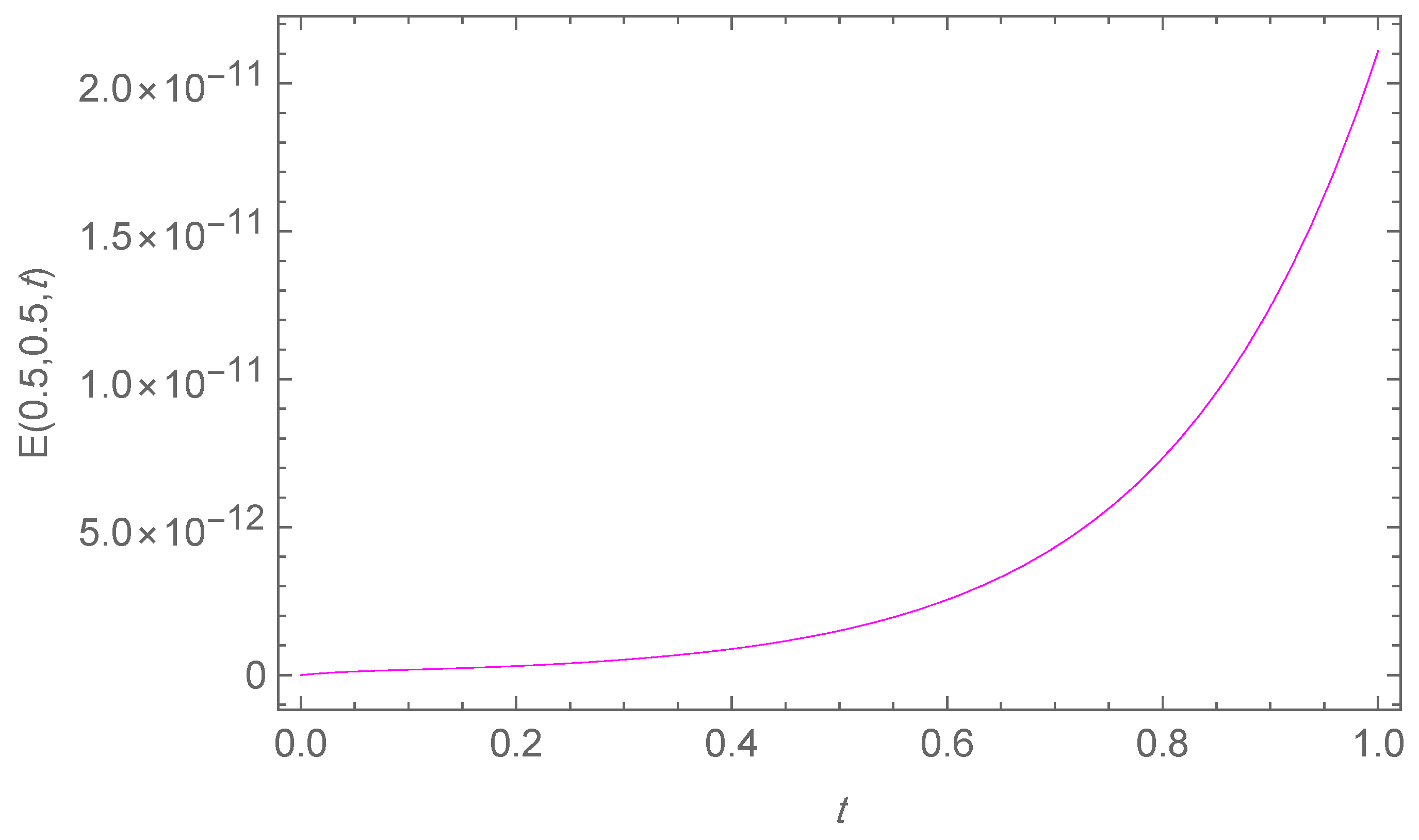
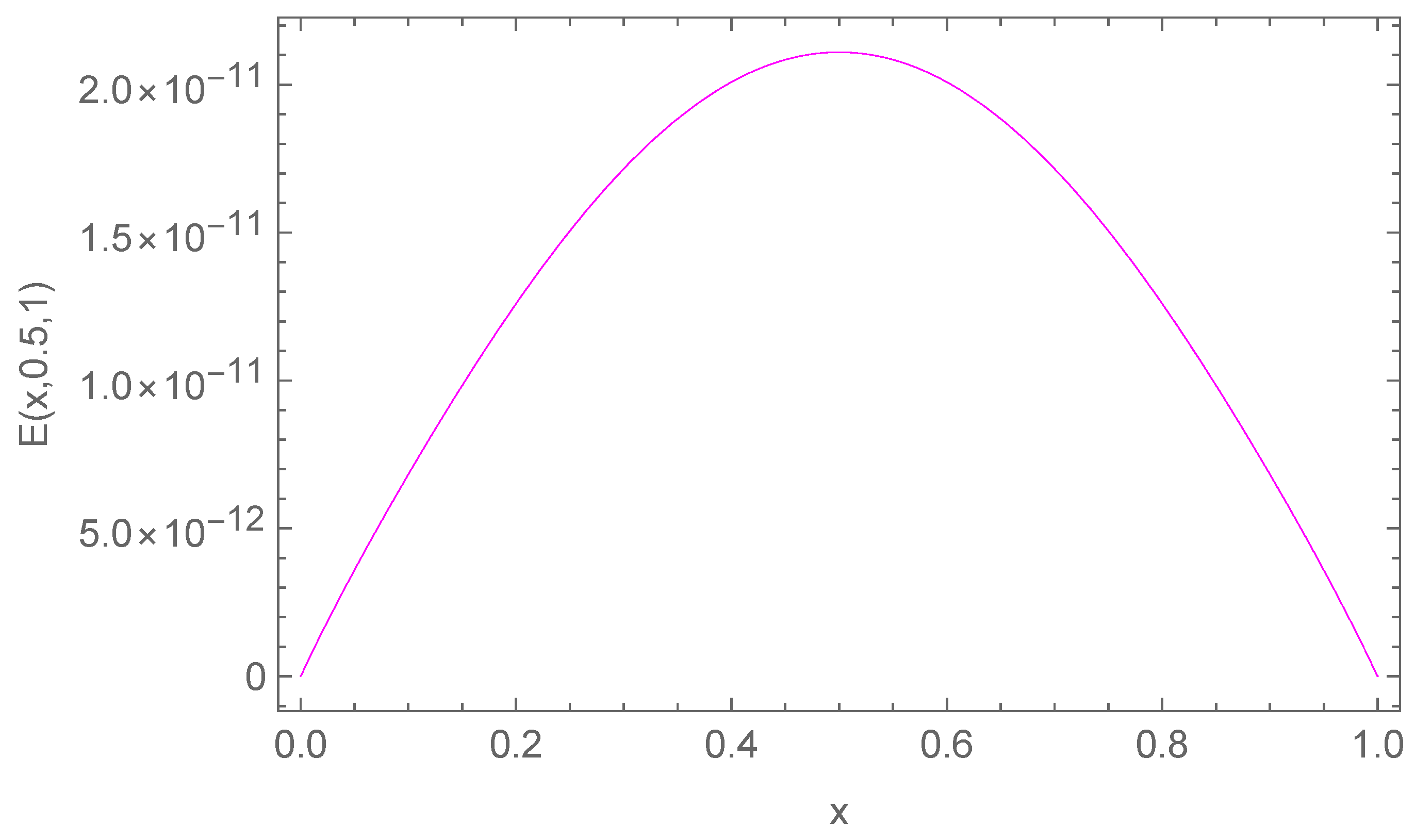
In Table 2, we present the maximum absolute errors obtained for Example 2, alongside the corresponding results from the Crank–Nicolson ADI Galerkin spectral method (CN-ADI-GSM) reported in [30]. Figure 8 illustrates the approximate solution u N ( x , y , t ) for the chosen parameter set N = 10 , α = 5 , β = 60 , λ 0 = r = 0 , λ 1 = λ 2 = 1 . The numerical solution closely matches the exact solution u ( x , y , t ) at selected points of y and t as shown in Figure 9. The associated absolute errors E ( x , y , t ) are depicted in Figure 10, Figure 11 and Figure 12 for the x y -plane, the t-direction, and the x-direction, respectively. The convergence decay curve in Figure 13 confirms the spectral accuracy of the method.
The presented results and graphs, across various test scenarios, confirm that the proposed method consistently yields solutions that closely approximate the exact values using only a small number of terms in the series expansion. This reflects its high accuracy and exponential convergence. The method’s robust algorithmic structure and efficient computational implementation significantly minimize numerical errors. Consequently, the high level of precision achieved makes the approach reliable for researchers and practitioners seeking accurate solutions in diverse scientific and engineering applications.

5.3. Computational Complexity Analysis

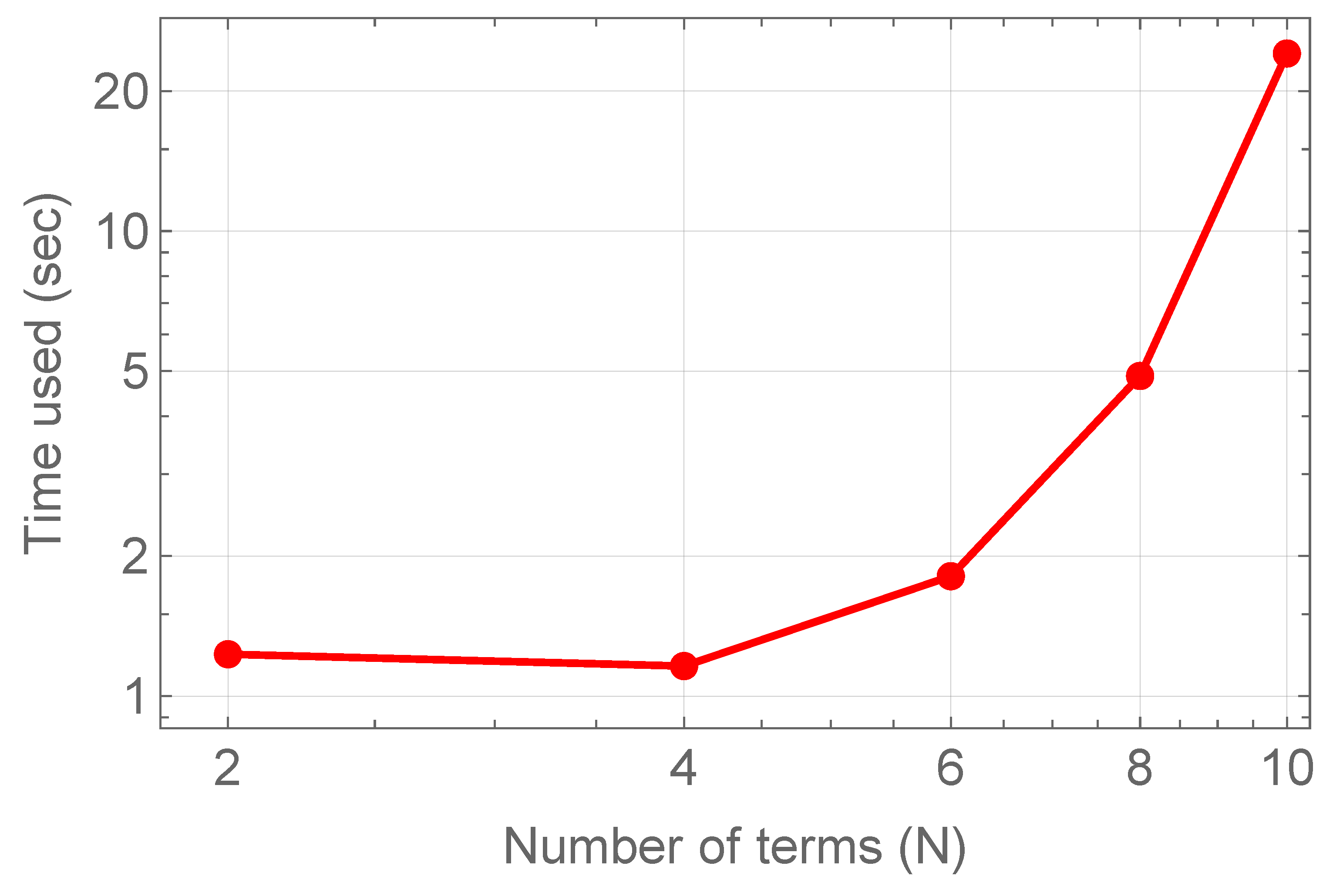
To further evaluate the performance of the proposed Legendre–Romanovski spectral collocation method, we analyzed the processing time based on the number of terms used in the approximate solution. In both the one- and two-dimensional cases, the approximate solution is expressed as a summation of orthogonal basis functions. A key advantage of this representation is that highly accurate results can be obtained with only a small number of terms, which significantly reduces the computational effort compared to many conventional approaches.
The one-dimensional results, summarized in Table 1 and illustrated in Figure 14, demonstrate that the required CPU time grows moderately with increasing N, following an empirical trend close to O ( N 1.6 ) . This indicates that the method can efficiently achieve spectral accuracy while keeping the computational cost low. In the two-dimensional case, presented in Table 3 and visualized in Figure 15, the timings increase more noticeably with the number of basis terms. However, the essential observation is that very accurate solutions are already achieved at relatively small values of ( N , M ) . This confirms that the method remains practical and effective for multidimensional problems, since only a limited number of basis functions is needed to reach high accuracy.
Overall, the complexity analysis highlights the efficiency of the proposed approach: a remarkably small number of terms is required to obtain an exponential convergence, making the method computationally attractive for solving nonlinear RDFDEs in both one and two dimensions.

6. Conclusions

In this study, we introduced a novel collocation-based spectral approach for solving one- and two-dimensional nonlinear RDFDEs. The scheme employs SL-G-L collocation for spatial discretization and a Romanovski-based collocation strategy for temporal discretization, reducing the problems to efficiently solvable algebraic systems. Numerical experiments confirmed the method’s spectral accuracy and effectiveness compared to existing approaches. The complexity analysis further demonstrated that remarkably accurate results can be achieved with only a few terms used in the approximate solution, underscoring the efficiency and practicality of the approach. Taken together, these results show that the proposed method combines accuracy, efficiency, and robustness, making it a valuable tool for numerically simulating nonlinear fractional models in science and engineering.

Author Contributions

Conceptualization, A.L., M.A.A. and S.S.; methodology, A.L., M.A.A. and S.S.; software, A.L., M.A.A. and S.S.; validation, A.L., M.A.A. and S.S.; formal analysis, A.L., M.A.A. and S.S.; investigation, A.L., M.A.A. and S.S.; resources, A.L., M.A.A. and S.S.; writing—original draft preparation, A.L., M.A.A. and S.S.; writing—review and editing, A.L., M.A.A. and S.S.; visualization, A.L., M.A.A. and S.S.; supervision, A.L., M.A.A. and S.S.; funding acquisition, M.A.A. All authors have read and agreed to the published version of the manuscript.

Funding

This work was supported and funded by the Deanship of Scientific Research at Imam Mohammad Ibn Saud Islamic University (IMSIU) (grant number IMSIU-DDRSP2502).

Data Availability Statement

The original contributions presented in this study are included in the article. Further inquiries can be directed to the corresponding author.

Conflicts of Interest

The authors declare no conflicts of interest.

Abbreviations

The following abbreviations are used in this manuscript:
DOFDEsDistributed order fractional differential equations
FDEsFractional differential equations
FPDEsFractional partial differential equations
RDFDEsReisz distributed order fractional differential equations
RJPsRomanovski–Jacobi polynomials
R-LFDRiemann–Liouville fractional derivative
SL-G-LShifted Legendre–Gauss–Lobatto

References

  1. Sarwar, N.; Asjad, M.I.; Sitthiwirattham, T.; Patanarapeelert, N.; Muhammad, T. A Prabhakar fractional approach for the convection flow of Casson fluid across an oscillating surface based on the generalized Fourier law. Symmetry 2021, 11, 2039. [Google Scholar] [CrossRef]
  2. Ionescu, C.; Lopes, A.; Copot, D.; Machado, J.A.T.; Bates, J.H.T. The role of fractional calculus in modeling biological phenomena: A review. Commun. Nonlinear Sci. Numer. Simul. 2017, 51, 141–159. [Google Scholar] [CrossRef]
  3. Raghavendran, P.; Gunasekar, T.; Balasundaram, H.; Santra, S.S.; Majumder, D.; Baleanu, D. Solving fractional integro-differential equations by Aboodh transform. J. Math. Comput. Sci. 2024, 32, 229–240. [Google Scholar] [CrossRef]
  4. Rihan, F.A. Fractional-order delay differential equations with predator-prey systems. In Delay Differential Equations and Applications to Biology; Springer: Berlin/Heidelberg, Germany, 2021; pp. 211–232. [Google Scholar]
  5. Alkandari, M.; Loutchko, D.; Luchko, Y. Anomalous Diffusion Models Involving Regularized General Fractional Derivatives with Sonin Kernels. Alex. Eng. J. 2025, 9, 363. [Google Scholar] [CrossRef]
  6. Caputo, M. Mean fractional-order-derivatives differential equations and filters. Ann. Dell’Universita Di Ferrara 1995, 41, 73–84. [Google Scholar] [CrossRef]
  7. Carrillo, J.A.; Fronzoni, S.; Süli, E. Finite element scheme for the fractional porous medium equation with fractional pressure. Numer. Math. 2025, 157, 1537–1614. [Google Scholar] [CrossRef]
  8. Ferrás, L.L. Fractional Derivatives: The ultimate operator for modelling complex viscoelastic materials? Fract. Calc. Appl. Anal. 2025. [Google Scholar] [CrossRef]
  9. Chechkin, A.V.; Gorenflo, R.; Sokolov, I.M. Retarding subdiffusion and accelerating superdiffusion governed by distributed-order fractional diffusion equations. Phys. Rev. E 2002, 66, 046129. [Google Scholar] [CrossRef]
  10. Caputo, M. Diffusion with space memory modelled with distributed order space fractional differential equations. Ann. Geophys. 2003, 46, 223–234. [Google Scholar] [CrossRef]
  11. Jian, H.-Y.; Huang, T.-Z.; Gu, X.-M.; Zhao, X.-L.; Zhao, Y.-L. Fast second-order implicit difference schemes for time distributed-order and Riesz space fractional diffusion-wave equations. Comput. Math. Appl. 2021, 94, 136–154. [Google Scholar] [CrossRef]
  12. Gao, Y.; Yin, D.; Zhao, B. A variable-order fractional constitutive model to characterize the rate-dependent mechanical behavior of soft materials. Fractal Fract. 2022, 6, 590. [Google Scholar] [CrossRef]
  13. Wang, Y.; Cai, M. Finite difference schemes for time-space fractional diffusion equations in one-and two-dimensions. Commun. Appl. Math. Comput. 2023, 5, 1674–1696. [Google Scholar] [CrossRef]
  14. Khan, M.A.; Alias, N.; Khan, I.; Salama, F.M.; Eldin, S.M. A new implicit high-order iterative scheme for the numerical simulation of the two-dimensional time fractional cable equation. Sci. Rep. 2023, 13, 1549. [Google Scholar] [CrossRef]
  15. Fei, M.; Huang, C. Galerkin–Legendre spectral method for the distributed-order time fractional fourth-order partial differential equation. Int. J. Comput. Math. 2020, 97, 1183–1196. [Google Scholar] [CrossRef]
  16. Luo, M.; Qiu, W.; Nikan, O.; Avazzadeh, Z. Second-order accurate, robust and efficient ADI Galerkin technique for the three-dimensional nonlocal heat model arising in viscoelasticity. Appl. Math. Comput. 2023, 440, 127655. [Google Scholar] [CrossRef]
  17. Srivastava, H.M.; Gusu, D.M.; Mohammed, P.O.; Wedajo, G.; Nonlaopon, K.; Hamed, Y.S. Solutions of general fractional-order differential equations by using the spectral Tau method. Fractal Fract. 2021, 6, 7. [Google Scholar] [CrossRef]
  18. Hadhoud, A.R.; Srivastava, H.M.; Rageh, A.A.M. Non-polynomial B-spline and shifted Jacobi spectral collocation techniques to solve time-fractional nonlinear coupled Burgers’ equations numerically. Adv. Differ. Equ. 2021, 2021, 439. [Google Scholar] [CrossRef]
  19. Amin, A.Z.; Abdelkawy, M.A.; Solouma, E.; Al-Dayel, I. A spectral collocation method for solving the non-linear distributed-order fractional Bagley–Torvik differential equation. Fractal Fract. 2023, 7, 780. [Google Scholar] [CrossRef]
  20. Ahmed, H.; Abd-Elhameed, W. Spectral Solutions of Specific Singular Differential Equations Using A Unified Spectral Galerkin-Collocation Algorithm. J. Nonlinear Math. Phys. 2024, 31, 42. [Google Scholar] [CrossRef]
  21. Lachin, A.; Abdelkawy, M.A.; Sathasivam, S. An efficient collocation method based on Legendre and Romanovski polynomials for solving Riesz distributed fractional differential equations. Alex. Eng. J. 2025, 129, 312–328. [Google Scholar] [CrossRef]
  22. Shen, J.; Tang, T.; Wang, L.-L. Spectral Methods: Algorithms, Analysis and Applications; Springer Science & Business Media: Berlin/Heidelberg, Germany, 2011; Volume 41. [Google Scholar]
  23. Abdelkawy, M.A.; Alyami, S.A. Legendre-Chebyshev spectral collocation method for two-dimensional nonlinear reaction-diffusion equation with Riesz space-fractional. Chaos Solitons Fractals 2021, 151, 111279. [Google Scholar] [CrossRef]
  24. Miller, K.S.; Ross, B. An Introduction to the Fractional Calculus and Fractional Differential Equations; Wiley–Blackwell: Hoboken, NJ, USA, 1993. [Google Scholar]
  25. Huang, X.; Fang, Z.-W.; Sun, H.-W.; Zhang, C.-H. A circulant preconditioner for the Riesz distributed-order space-fractional diffusion equations. Linear Multilinear Algebra 2022, 70, 3081–3096. [Google Scholar] [CrossRef]
  26. Zhao, J.; Zhang, Y.; Xu, Y. Implicit Runge–Kutta and spectral Galerkin methods for Riesz space fractional/distributed-order diffusion equation. Comput. Appl. Math. 2020, 39, 47. [Google Scholar] [CrossRef]
  27. Izadi, M.; Veeresha, P.; Adel, W. The fractional-order marriage–divorce mathematical model: Numerical investigations and dynamical analysis. Eur. Phys. J. Plus 2024, 139, 205. [Google Scholar] [CrossRef]
  28. Nazari, J.; Heydari, M.H.; Hosseininia, M. Romanovski–Jacobi polynomials for the numerical solution of multi-dimensional multi-order time fractional telegraph equations. Results Phys. 2023, 53, 106937. [Google Scholar] [CrossRef]
  29. Abdelkawy, M.A.; Menaem, A.A.; Matoog, R.T.; Tedjani, A.H. Romanovski–Jacobi spectral collocation schemes for distributed order differential problems. Alex. Eng. J. 2024, 101, 98–107. [Google Scholar] [CrossRef]
  30. Zhang, H.; Liu, F.; Jiang, X.; Zeng, F.; Turner, I. A Crank–Nicolson ADI Galerkin–Legendre spectral method for the two-dimensional Riesz space distributed-order advection–diffusion equation. Comput. Math. Appl. 2018, 76, 2460–2476. [Google Scholar] [CrossRef]
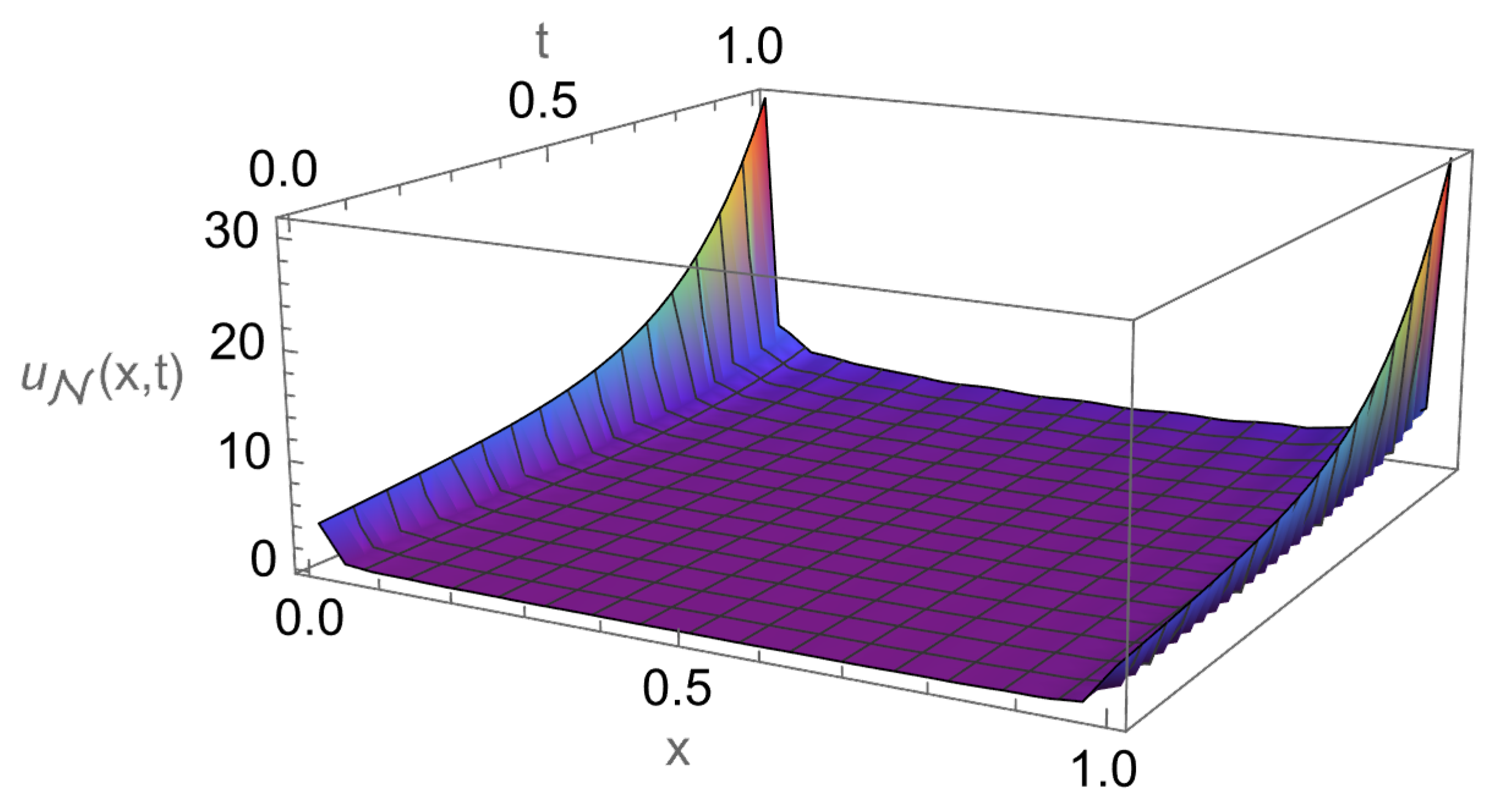
Figure 1. Approximate solution of Example 1.
Mathematics 13 03425 g001
Figure 2. Absolute error distribution for Example 1.
Mathematics 13 03425 g002
Figure 3. Exact vs. numerical solutions along the x-direction for Example 1.
Mathematics 13 03425 g003
Figure 4. Exact vs. numerical solutions along the t-direction for Example 1.
Mathematics 13 03425 g004
Figure 5. Absolute error along the t-direction when x = 0.5 for Example 1.
Mathematics 13 03425 g005
Figure 6. Absolute error along the x-direction when t = 0.5 for Example 1.
Mathematics 13 03425 g006
Figure 7. Convergence decay for Example 1.
Mathematics 13 03425 g007
Figure 8. Approximate solution of Example 2.
Mathematics 13 03425 g008
Figure 9. Exact vs. numerical solutions along the x-direction for Example 2.
Mathematics 13 03425 g009
Figure 10. Absolute error for Example 2.
Mathematics 13 03425 g010
Figure 11. Absolute error along the t-direction when x = y = 0.5 for Example 2.
Mathematics 13 03425 g011
Figure 12. Absolute error along the x-direction when y = 0.5 , t = 1 for Example 2.
Mathematics 13 03425 g012
Figure 13. Convergence decay for Example 2.
Mathematics 13 03425 g013
Figure 14. CPU time versus number of terms N for the one-dimensional case of Example 1.
Mathematics 13 03425 g014
Figure 15. CPU time versus number of terms ( N , M ) for the two-dimensional case of Example 2.
Mathematics 13 03425 g015
Table 1. Maximum absolute errors and CPU time for Example 1.
N α = 5 , r = 4.9 α = 5 , r = 5 Average CPU
β = 45 β = 60 β = 45 β = 60 Time (s)
20.24360.19800.24070.19631.23
4 1.0587 1.45251.04851.43951.16
5 5.89 × 10 4 7.60 × 10 4 6.57 × 10 6 9.53 × 10 6 1.50
6 2.30 × 10 4 1.30 × 10 4 1.48 × 10 6 5.57 × 10 7 1.81
8 8.48 × 10 5 1.09 × 10 5 8.58 × 10 8 1.18 × 10 9 4.88
10 5.13 × 10 5 5.92 × 10 6 8.76 × 10 9 2.58 × 10 11 24.095
Table 2. Maximum absolute errors for Example 2.
Romanovski Legendre Collocation MethodCN-ADI-GSM [30]
( N , M ) α = 5 , β = 60 , λ 0 = 0 α = 5 , β = 60 , λ 0 = 1 λ 0 = 0 , r = 0
r = 0 r = 4 . 9 r = 0 N L 2 errors
(4, 4)0.56960.57090.6696
(5, 5) 1.95 × 10 7 2.09 × 10 5 3.73 × 10 7 8 5.5639 × 10 5
(6, 6) 8.11 × 10 8 4.57 × 10 5 1.20 × 10 7 16 1.6841 × 10 5
(8, 8) 9.32 × 10 10 6.71 × 10 6 7.77 × 10 10 32 1.0670 × 10 6
(10, 10) 2.11 × 10 11 4.52 × 10 6 5.90 × 10 13 64 2.4951 × 10 8
Table 3. CPU time and maximum absolute errors in the two-dimensional case of Example 2.
α = 5 , β = 60 , λ 0 = 0 , r = 5
( N , M ) ErrorTime Used (s)
(2, 2)    0.0156     1.11
(4, 4)    0.5696     5.66
(5, 5)    1.95 × 10 7    44.50
(6, 6)    1.20 × 10 7    232.30
(8, 8)    9.32 × 10 10    1810.41
Disclaimer/Publisher’s Note: The statements, opinions and data contained in all publications are solely those of the individual author(s) and contributor(s) and not of MDPI and/or the editor(s). MDPI and/or the editor(s) disclaim responsibility for any injury to people or property resulting from any ideas, methods, instructions or products referred to in the content.