Optimization of Rainfall Monitoring Network in Northern Thailand Through Centrality-Weighted Graph Analysis with Simulated Annealing

Abstract

The development of an optimally designed rain gauge network is crucial for achieving cost-efficient operation and maintenance and maintaining the overall accuracy of rainfall estimation. Traditional rainfall monitoring network optimization relies primarily on statistical methods without consideration of the underlying network configuration. This study presents a hybrid optimization approach integrating graph theory related to centrality (betweenness and clustering coefficient), minimum spanning tree (MST) and simulated annealing (SA) for monitoring station reduction. The proposed hybrid MST-SA algorithm with adaptive graph weighting applies to 317 monitoring stations in the northern Thailand using 11 years of wet-season rainfall data (2012–2022). Six main scenarios, involving the removal of 5 to 30 stations, are analyzed through the adjustment of the trade-off parameter between correlation and centrality. The results indicate that the proposed method outperforms the approach based solely on the correlation coefficient. This hybrid MST-SA approach achieves faster convergence and effectively preserves the continuity of spatial information throughout the domain. Furthermore, as the number of reduced stations increases, the influence of centrality becomes increasingly pronounced compared to that obtained solely from correlation analysis.

1. Introduction

Current extreme climate events pose significant threats to both natural and human systems. Such events are anticipated to exemplify the impacts of climate change. These climatic shifts contribute to the increasing intensity, frequency of rainfall, and irregular monsoon patterns, as well as more severe and prolonged droughts in some areas [1]. Rainfall data serves as a critical component for analyzing the spatial and temporal patterns of precipitation changes in response to climate change. Such analysis can essentially facilitate water resources planning, rainfall-runoff forecasting, and reservoir operation. In relation to this, rain gauge networks are typically established to enable the direct measurement of rainfall, capturing both the spatial and temporal variability of precipitation within a catchment area. Given the inherently high variability of rainfall and its complex spatial distribution, the development of a well-designed rain gauge network is important for cost-effective operation and maintenance while enhancing the overall accuracy of rainfall data. A wide range of techniques have been proposed for the optimal design of rain gauge station networks. These methods primarily include statistical methods [2,3], entropy-based techniques [4,5,6], satellite-based remote sensing technologies [7,8], machine learning [9,10], and optimization approaches.

Among them, statistical methodologies constitute some of the most extensively developed approaches for rain gauge network design. These include copula, cross-correlation analysis, generalized least squares, and variance reduction techniques. Kriging-based geostatistical methods, in particular, are the most widely applied for both the design and evaluation of rain gauge networks. The kriging techniques alone were employed in earlier studies due to its well-balanced combination of flexibility and statistical optimality. The Best Linear Unbiased Estimator (BLUE) property of kriging under the unbiasedness condition ensures that the minimum variance of estimation error is achieved. This property makes it particularly effective in identifying stations within specific regions that do not substantially contribute to reducing the estimated variance. It also provides guidance for the strategic placement of additional stations at selected locations to minimize the overall estimation error. Kassim and Kottegoda [11] compared simple kriging and disjunctive kriging in selecting the optimal configuration of rain gauges over an area of approximately 1800 square kilometers surrounding Birmingham, United Kingdom, using rainfall data from 13 stations recorded during storm events. Adhikary et al. [12] employed the variance reduction method within the framework of ordinary kriging (OK), utilizing standard parametric variogram functions for the design of a rain gauge network in the Middle Yarra River catchment in Victoria, Australia. Their study was further extended through the application of ordinary cokriging and kriging with external drift (KED), incorporating digital elevation data as a secondary variable, to interpolate monthly rainfall in two Australian catchments [13]. These two cokriging models outperformed deterministic interpolation methods.

Another advancement of kriging within the context of optimal network design lies in its integration with other optimization techniques. In such a framework, the kriging variance can be employed as an objective function or performance metric, enabling more effective and systematic network optimization. Because station design problems are often complex, large-scale, and nonlinear, conventional and simple heuristic optimization methods are generally unsuitable for large-scale spatial optimization. Consequently, metaheuristic approaches such as particle swarm optimization, genetic algorithms (GA), and simulated annealing (SA), are commonly utilized to address these challenges. The study by Aziz et al. [14] applied a particle swarm optimization technique integrated with geostatistics to design a rain gauge network in Johor State. The approach minimized kriging variance by examining other meteorological variables, including rainfall, elevation, humidity, solar radiation, temperature, and wind speed. While the Artificial Bee Colony (ABC) algorithm was utilized with the block OK approach by the work of Attar et al. [15] for the rain gauge network design in the southwestern part of Iran. A key focus of their study was to mitigate the curse of dimensionality via a hybrid framework that combines various objective functions with the ABC algorithm. Bayat et al. [16] introduced a two-phase methodology to analyze the spatiotemporal structure of precipitation within the Namak Lake watershed in central Iran, based on three decades of data collected from 105 rainfall monitoring stations. In the initial phase, the entropy was employed as a decision-making tool to determine the optimal number of rain gauge stations required for effective coverage. The subsequent phase coupled GA with geostatistical approaches, namely OK and Bayesian maximum entropy, to optimize the spatial configuration of the rain gauge network. This optimization process was guided by three objective functions, which are the minimization of the expected estimation variance, the minimization of the mean squared error, and the maximization of the coefficient of determination ($R^2$). Pardo-Igúzquiza [17] combined the kriging method with SA to derive an optimal rainfall configuration. The objective function was formulated based on two key criteria, which are the kriging variance estimated from synthetic rainfall datasets and the associated economic cost. The optimization process addressed two scenarios, which are the optimal selection of a subset from the existing stations and the optimal augmentation of the current network. The use of SA was also employed in the work by Wadoux et al. [18]. They extended the geostatistical interpolation of rainfall data through the use of the KED model by merging rain gauge and radar data in the north of England for a one-year period. The rain gauge sampling design was optimized by minimizing the space-time average KED variance. Omer et al. [19] compared SA and GA methods coupled with OK and universal kriging (UK) based on data from more than 90 stations over the period from 1998 to 2019. The SA exhibits a lower average kriging variance (AKV) compared to GA when adding the optimal or removing the redundant locations from the monitoring network.

From another perspective on station reduction, the station network can be represented within a graph-based framework. Donges et al. [20] and Scarsoglio et al. [21] investigated the placement of monitoring stations in climate networks, where nodes correspond to stations and edges capture the relationships between station pairs. Their studies utilized graph representations solely for descriptive purposes, rather than as a means of facilitating station reduction. Several studies have also explored the integration of correlation analysis with graph-theoretic approaches for various applications related to climate patterns. Building upon the concept of correlation-based graph construction, Ebert-Uphoff and Deng [22] introduced correlation graphs that synthesize traditional graph structures with correlation coefficients derived from climate data. This foundational work was further developed by [23], who utilized correlation matrices computed from data correlation coefficients as weight matrices for connected graphs, leading to the identification of small-world network properties within the underlying data structure. In 2009, Sukharev et al. [24] applied k-means clustering and graph partitioning algorithms to analyze correlation structures of variable pairs through pointwise correlation coefficients and canonical correlation analysis. Traditional graph approaches often depend on correlation coefficients, which may fail to capture the full structural complexity and hierarchy of networks, while these methods typically cluster nearby stations exhibiting similar meteorological patterns, they may overlook deeper, less apparent interrelationships. To date, numerous studies have employed graph-based approaches primarily to represent various types of networks, particularly correlation or climate networks. Clustering techniques have also been frequently utilized to identify influential nodes or to extract specific network properties. However, there remains a noteworthy gap in the existing research, which stems from the lack of a systematic integration of fundamental graph-theoretic concepts, such as connectedness and centrality, into station design. The application of these concepts can help preserve the continuity of spatial information across the domain when certain stations are removed.

The primary objective of this research is the augmentation of the SA optimization technique through the integration of the graph theory, with the AKV serving as the objective function. In the preprocessing stage, potential station removals are determined via the minimum spanning tree (MST) problem, where the importance of each station within the network is assessed using graph-theoretic weights. Instead of relying solely on correlation coefficients to compute these weights, we incorporate centrality analysis by including both the clustering coefficient and betweenness centrality. The clustering coefficient quantifies the local interconnectedness of node’s neighbors, whereas the betweenness centrality measures the frequency with which a station appears on the shortest paths between other nodes in the network. To evaluate performance, monthly rainfall data from 317 stations across Thailand over the period 2012–2022 were employed, with 9 years (2012–2020) allocated for training and 2 years (2021–2022) for validation.

The remainder of this paper is organized as follows. Section 2 describes the study area and the data utilized for the analysis. Section 3 provides a description of techniques related to our proposed method. Section 4 presents the detailed algorithm of the hybrid MST-SA approach with adaptive graph weighting. In Section 5, the performance of our proposed method is discussed. Conclusions of this study are drawn in Section 6. List of all variables and parameters is provided in

Table 1. List of all variables and parameters.

Symbols	Description
V	Set of vertices
E	Set of edges
$G=(V,E)$	Graph that has nodes as elements in set V and edges in set E
$w_{ij}$	Weight of the edge between nodes i and j
$cut\left(G\right)$	Cut set of graph G
$cc\left(v\right)$	Clustering coefficient of vertex v
$e\left(v\right)$	The number of edges between neighbors of v
$deg\left(v\right)$	The number of edges that connect to vertex v
$b\left(v\right)$	Betweenness value of vertex v
$\rho (i,j)$	The total number of shortest paths from i to j
${\rho }_v(i,j)$	The number of shortest paths from i to j that pass through v
$L\left(G\right)$	Line graph of graph G
$x_{ij}$	Binary decision variable
${\mathbf{s}}_i$	Location at node i
$Z\left({\mathbf{s}}_i\right)$	Data sampling at node i
${\lambda }_i$	Kriging weight assigned to $Z\left({\mathbf{s}}_i\right)$
${\sigma }_k^2$	Kriging variance
T	SA temperature parameter
$\eta$	SA cooling rate
$\alpha$	Trade-off parameter between correlation and centrality
S	Set of all stations
R	Set of removed stations
$M^{*}$	Set of the removing stations ordered by descending kriging variance
$\delta$	Weight-adjustable parameter
$t_{max}$	Maximum iteration

.

2. Study Area and Data

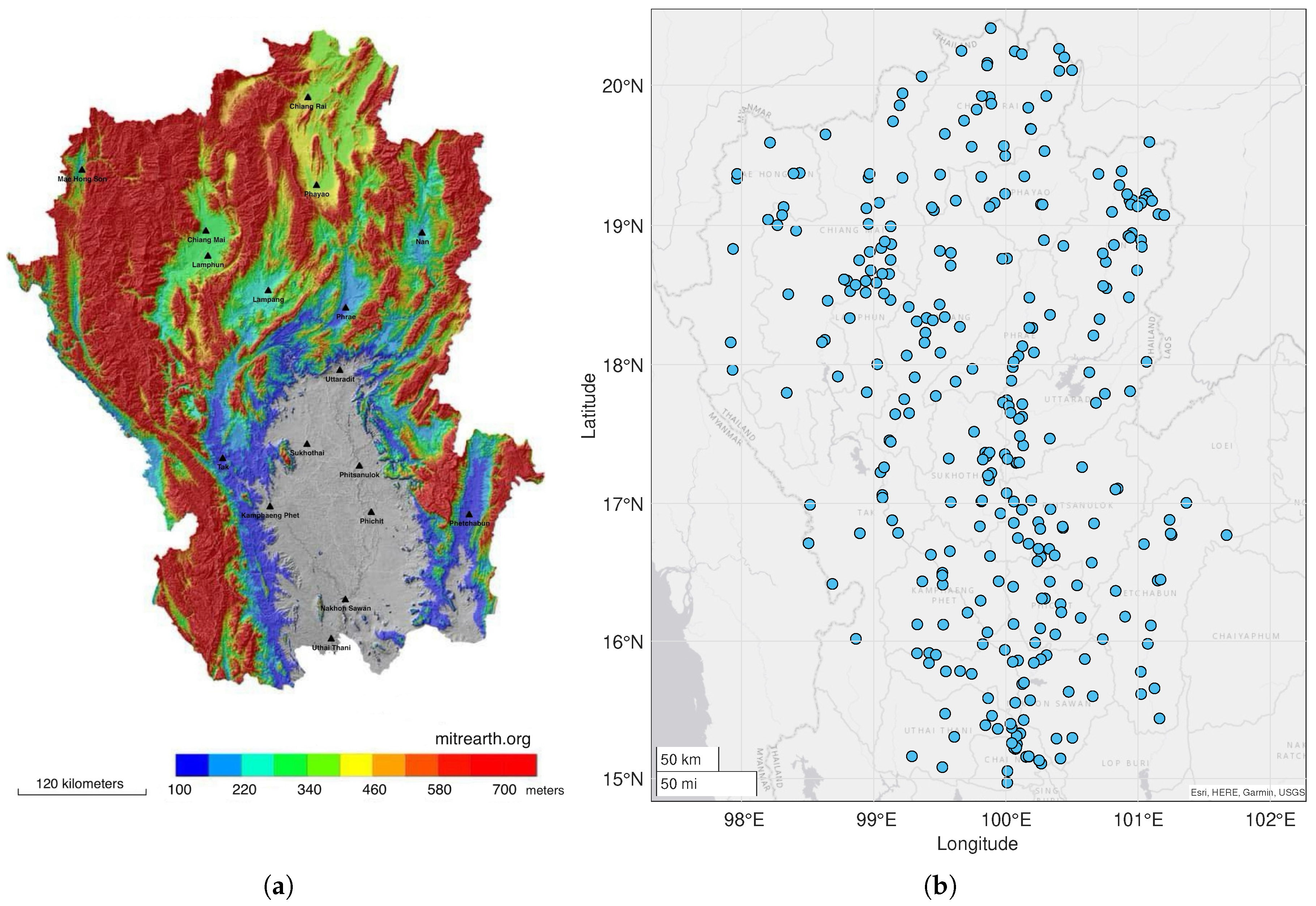
Our domain of study is located in the northern region of Thailand, which lies between latitudes 14°56′17″–20°27′5″ North and longitudes 97°20′38″–101°47′31″ East, covering 17 provinces with an area of 172,277 km². The northern region of Thailand can be divided into upper and lower parts. Topographically, see Figure 1a (adapted from www.mitrearth.org), the upper north is characterized as a mountainous zone, dominated by north–south oriented ranges. Between these ranges lie fertile intermontane basins and river valleys, which give rise to four principal tributaries (Ping, Wang, Yom and Nan) that form the headwaters of the Chao Phraya River in central Thailand. In contrast, the lower-north region serves as a transition zone between the rugged highlands of the upper north and the flat central plain, characterized by broad river valleys and extensive floodplains.

The annual rainfall variation across this region is highly heterogenous, with between 70% and 80% of its total annual rainfall occurring during the wet season from May to September. These rainfalls are influenced from the Intertropical Convergence Zone (ITCZ) and the monsoon trough, which dominate during the wet season. Two primary mechanisms account for most of the rainfall include the southwest monsoons prevailing from mid-May to early-June, and westward-propagating tropical stroms originating in the south China sea and western Pacific, which reach their peak in September. Notably, rainfall associated with tropical storms contributes nearly 70% of the total rainfall in Thailand during September [25].

Monthly data used in this study includes rainfall, humidity, atmospheric pressure, and temperature, were obtained from the Thai Meteorological Department (TMD) and the National Hydroinformatics and Climate Data Center, developed by the Hydro-Informatics Institute (HII). To mitigate the effects of misleading correlations that may arise from prolonged periods without rainfall, our analysis focuses on wet-season characteristics (April–October) for the years 2012–2022. Within the 11-year dataset, the first 9 years served as the training dataset, while the final 2 years are treated as the interpolation testing set. Each dataset was attained from 317 monitoring stations as shown in Figure 1b, consisting of both human-operated and self-automated stations. Based on the frequency of westward-propagating tropical storms, this has led to a high density of rain gauge networks on the eastern side of the study region. Another dense cluster is noticeable in the central area, where major cities and densely populated communities are situated. On the other hand, the network is less concentrated along the western border adjacent to Myanmar, as this region is characterized by high mountain ranges and sparse population.

Table 2. Descriptive statistics of monthly mean daily rainfall (mm/day) from 2012 to 2022.

Month	Mean	Max	Min	SD	Var	Skewness	Kurtosis
April	58.31	420.60	0	32.49	1055.51	2.15	9.68
May	87.93	909.00	0	34.93	1220.35	1.97	10.50
June	88.81	849.00	0	36.68	1345.14	3.07	21.99
July	125.24	820.40	0	46.88	2197.52	1.16	4.87
August	159.21	636.00	0	57.30	3283.63	1.18	5.89
September	148.42	719.60	0	58.29	3398.28	1.67	7.69
October	92.70	403.00	0	33.61	1129.44	1.66	8.50

presents the statistical summary of the mean daily rainfall for each month across 317 rain gauges. Throughout the seven-month study period spanning 11 years, higher monthly mean daily rainfall values were observed during July to September, with the peak value of 159.21 mm recorded in August. In contrast, the lowest monthly mean daily rainfall, amounting to 58.31 mm, occurred in April. Moreover, the standard deviation of the mean daily rainfall data were generally consistent with the mean. In other words, higher mean values tended to correspond to higher standard deviations. All months in the study exhibit positive skewness, indicating that the distribution of rainfall values across the domain is right-skewed. This suggests that a small number of stations experience relatively high rainfall intensities compared to the majority of observations.

3. Preliminaries

This section presents fundamental concepts related to graph theory and optimization and their uses in this study. Topics include some graph definitions, centrality measures, the minimum spanning tree, and simulated annealing.

3.1. Graph Definitions

Definition 1

(Ref. [26]). Given an undirected and connected graph $G=(V,E)$, where V is the set of vertices and E is the set of edges. Let $w_{ij}$ denote the weight of the edge between nodes i and j, where $(i,j)\in E$. Let $\tau =(V,E_{\tau })$ be a spanning tree of G. A tree ${\tau }^{\prime }\subseteq \tau$ is said to be minimum spanning tree (MST) if its total edge weight is minimized among all possible spanning trees of G, i.e.,

$$\sum _{(i,j)\in E_{{\tau }^{\prime }}}{w}_{ij}\le \sum _{(i,j)\in E_{\tau }}{w}_{ij}.$$

(1)

Definition 2

(Ref. [27]). A set of vertices is a cut set if its deletion increases the number of connected components in a graph. The cut set of graph G is denoted $cut\left(G\right)$.

A cut set refers to a set of nodes whose removal results in the division of a connected graph into two or more disconnected components. Examining cut sets enables the identification of critical links or stations within the monitoring network, highlighting points where failure could disrupt the overall connectivity and significantly hinder data collection or communication.

Definition 3

(Ref. [28]). The clustering coefficient of vertex v, denoted by $cc\left(v\right)$, is defined as the number of edges between the vertices within the immediate neighborhood of the vertex divided by the number of all possible edges between them. It can be computed by

$$cc\left(v\right)={\displaystyle \frac{2·e\left(v\right)}{deg\left(v\right)·\left(deg\right(v)-1)}}$$

(2)

where $e\left(v\right)$ is the number of edges between neighbors of v and $deg\left(v\right)$ is the number of edges that connect to vertex v.

Clustering Coefficient is a metric assessing how strongly nodes in a graph tend to form clusters. It reflects the probability that two neighbors of a given node are also directly connected to each other. A low clustering coefficient signifies the sparse local connectivity of a node, indicating that the node’s neighbors are poorly connected to one another, thereby reducing the node’s embeddedness within densely interconnected substructures.

Definition 4

(Ref. [29]). The betweenness of vertex v, denoted by $b\left(v\right)$, is defined as the proportion of the shortest paths between every pair of vertices that pass through the given vertex v towards all the shortest paths. It can be written as

$$b\left(v\right)=\sum _{i\ne j\ne v}{\displaystyle \frac{{\rho }_v(i,j)}{\rho (i,j)}}$$

(3)

where i and j are two distinct vertices of G not equal to v, ${\rho }_v(i,j)$ is the number of shortest paths from i to j that pass through v, and $\rho (i,j)$ is the total number of shortest paths from i to j.

Betweenness centrality measures how frequently a node appears on all shortest paths between other pairs of nodes. Nodes with high betweenness are vital for facilitating the flow of information throughout the network, as they frequently serve as bridges along crucial communication routes.

The clustering coefficient and betweenness together offer valuable insights into the significance of various locations and connections within the weather monitoring network, thereby aiding in the identification of optimal sites for station deployment. This complementary combination allows our optimization framework to simultaneously manage global connectivity (from betweenness) and local redundancy (from clustering coefficient), which cannot achieve by a single metric alone.

Definition 5

(Ref. [30]). Given an undirected graph G, the line graph $L\left(G\right)$ has the edges of G as its vertices, i.e., $V\left(L\right(G\left)\right)=E\left(G\right)$. Two vertices in $L\left(G\right)$ are adjacent if and only if the corresponding edges in G share a common endpoint.

A line graph is a transformed representation of the original graph where edges are converted to nodes, enabling the analysis of edge properties. By applying centrality measures to line graphs, we can assess the importance of edges, i.e., the relationships between nodes in the original graph.

3.2. Minimum Spanning Tree Problem

The MST problem aims to find a subset of edges in a connected and undirected graph $G=(V,E)$ that connects all vertices together, without any cycles and with the minimum possible total edge weight. The common formulation of MST can be represented in the form of linear integer programming as follows:

$$\begin{array}{cc}\hfill & \mathrm{minimize}\sum _{(i,j)\in E}{w}_{ij}{x}_{ij}\hfill \end{array}$$

(4)

$$\begin{array}{cc}\hfill & \mathrm{subject}\mathrm{to}\sum _{(i,j)\in E}{x}_{ij}=\left|V\right|-1\hfill \end{array}$$

(5)

$$\begin{array}{cc}\hfill & \sum _{i\in V^{*},j\in V\setminus V^{*},(i,j)\in E}{x}_{ij}\ge 1,\forall V^{*}\subset V,V^{*}\ne \varnothing \hfill \end{array}$$

(6)

$$\begin{array}{cc}\hfill & x_{ij}\in \{0,1\},\forall (i,j)\in E.\hfill \end{array}$$

(7)

Each edge $(i,j)\in E$ has a weight $w_{ij}>0$. We define binary decision variables

$$x_{ij}=\left\{\begin{array}{cc}1\hfill & \mathrm{if}\mathrm{edge}(i,j)\mathrm{is}\mathrm{included}\mathrm{in}\mathrm{the}\mathrm{MST},\hfill \\ 0\hfill & \mathrm{otherwise}.\hfill \end{array}\right.$$

(8)

Constraints (5) and (6) keep the graph as a tree and ensure it remains connected, respectively.

The application of MST problem for node selection problems is appropriate when the objective is to maintain connectivity while minimizing total edge weights.

3.3. Ordinary Kriging

Suppose that $\{Z\left(\mathbf{s}\right):\mathbf{s}\in D\subset {\mathbb{R}}^d\}$ is a spatial random process over a spatial domain D and $d\ge 1$. Let $\{Z\left({\mathbf{s}}_1\right),Z\left({\mathbf{s}}_2\right),\dots ,Z\left({\mathbf{s}}_n\right)\}$ be a collection of samples at observed locations $1,2,\dots ,n$. The estimate $Z^{*}\left(\mathbf{s}\right)$ at non-visited site $\mathbf{s}$ can be expressed as a linear combination of n measurements

$$Z^{*}\left(\mathbf{s}\right)=\sum _{i=1}^n{\lambda }_{i}Z\left({\mathbf{s}}_i\right)$$

(9)

where ${\lambda }_i$ represents the kriging weight assigned to $Z\left({\mathbf{s}}_i\right)$.

The OK approach satisfies the property of intrinsically stationarity, in which the expected value of the difference between $Z\left(\mathbf{s}\right)$ and $Z(\mathbf{s}+\mathbf{h})$ is zero, and the variance of this difference is determined by the lag vector $\mathbf{h}$. Moreover, the kriging variance, which is the variance of the estimation error, can be formulated using the semivariogram, which describes the covariance structure among the sampled data points. It is given by [31]

$${\sigma }_k^2\left(\mathbf{s}\right)=Var[Z^{*}\left(\mathbf{s}\right)-Z\left(\mathbf{s}\right)]=2\sum _{i=1}^n{\lambda }_i\gamma ({\mathbf{s}}_i-\mathbf{s})-\sum _{j=1}^n\sum _{j=1}^n{\lambda }_j{\lambda }_i\gamma ({\mathbf{s}}_i-{\mathbf{s}}_j).$$

(10)

By employing the Lagrange multiplier technique on Equation (10) under the unbiasedness constraint ${\sum }_{i=1}^n{\lambda }_i=1$, we obtain

$$\sum _{i=1}^n{\lambda }_i\gamma ({\mathbf{s}}_i-\mathbf{s})+\mu =\gamma ({\mathbf{s}}_i-\mathbf{s})$$

(11)

where $\mu$ denotes the Lagrange multiplier, and the kriging weight can be computed from [32]

$$\widehat{\gamma }\left(\mathbf{h}\right)={\displaystyle \frac{1}{2N\left(\mathbf{h}\right)}}\sum _i^{N\left(\mathbf{h}\right)}(Z\left({\mathbf{s}}_i\right)-Z({\mathbf{s}}_i+\mathbf{h}))$$

(12)

where $N\left(\mathbf{h}\right)$ represents the number of distinct pairs separated by the lag vector $\mathbf{h}$. Under the assumption of isotropy, the semivariogram estimator $\widehat{\gamma }\left(\mathbf{h}\right)$ depends only on the Euclidear distance $h=\Vert \mathbf{h}\Vert$. Based on the empirical semivariogram, the spatial continuity over the domain can be approximated using smooth parametric models, including exponential, spherical and Gaussian functions. In this study, we adopt the exponential model, expressed as

$${\gamma }^{*}\left(h\right)=\left\{\begin{array}{cc}{c}_0+c_1\left(1-exp\left(-{\displaystyle \frac{h}{c_2}}\right)\right),\hfill & h>0\hfill \\ 0,\hfill & h=0\hfill \end{array}\right.$$

(13)

where the parameters $c_0,c_1$ and $c_2$ are nonnegative and are determined by applying the least squares method to achieve their optimal values.

3.4. Simulated Annealing

The SA technique is a probabilistic heuristic optimization method introduced by Kirkpatrick et al. [33] and Černý, V. [34]. The algorithm is inspired by the metallurgical process of annealing, wherein a material is rapidly heated and subsequently gradually cooled until it attains the ground state. Throughout this process, the atoms within the metal rearrange themselves toward a configuration that minimizes the system’s energy. In the optimization analogy, the atomic or molecular structure represents the configuration of sampling points, while the objective function reflects the energy level of the system. The SA algorithm aims to prevent entrapment in a local optimal solution by utilizing the Metropolis criterion and generating new candidate solutions within the vicinity of the current solution. The algorithm’s performance is significantly influenced by the selection of the cooling schedule and the neighborhood structure. The SA algorithm based on the linear cooling schedule is detailed in Algorithm 1.

Algorithm 1 Simulated Annealing

Initialize the solution $\theta$ and the initial temperature T Set the cooling rate $\eta$, $0<\eta <1$ while termination is not satisfied do     Generate a candidate solution ${\theta }^{*}$     Calculate the change in energy $\Delta F=f\left({\theta }^{*}\right)-f\left(\theta \right)$     if $\Delta F<0$ then         Accept the candidate solution ${\theta }^{*}$     else         Accept ${\theta }^{*}$ with probability $P=e^{-\Delta F/T}$     end if     Update the current solution $\theta ={\theta }^{*}$     Update the temperature $T^{*}=\eta T$ end while Return the optimal solution

4. Methodology

In this section, we present the procedure of the removing redundant monitoring station problem.

4.1. Graph Creation

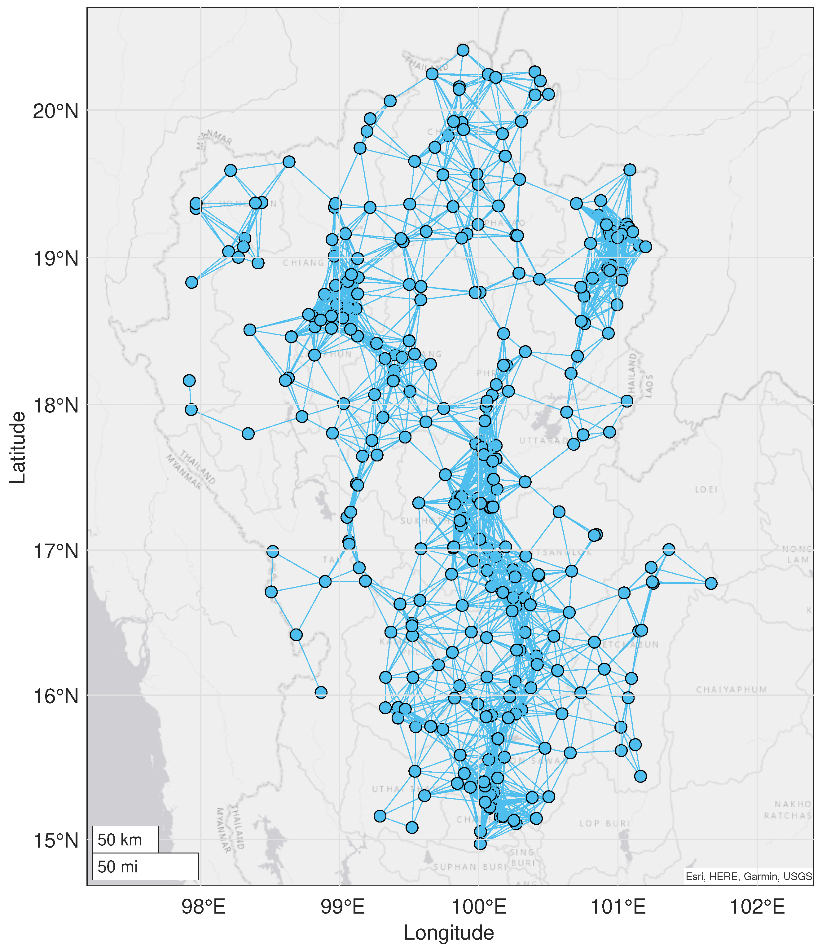
In this framework, each station’s location is modeled as a node of the graph, represented by $G=(S,E_S)$, where S is set of all stations and $E_S$ is set of all edges between them. An undirected edge is established between any pair of stations if their separation distance is less than a predefined threshold, which is the minimum distance allowing all stations in our study to form a connected graph. The minimum predefined threshold to create the graph G in our study area is $D=48.2175$, which is demonstrated in Figure 2.

Since we intend to apply the MST strategy for selecting which nodes to retain in the graph, it is necessary to assign low weight values to edges adjacent to important stations. In other words, one assigns high weight values to edges connected to unnecessary stations. In our study, the weights consist of two main components. One is assigned by Pearson’s correlation coefficient [35] of rainfall measurements between each pair of connected stations $(i,j)\in E_S$ denoted by $C(i,j)$. The other part is related to centrality, which is computed from betweenness, $b\left(\right(i,j\left)\right)$, and clustering coefficient, $cc\left(\right(i,j\left)\right)$, through line graph $L\left(G\right)$. The proposed adaptive weight used in this study is given by

$$w_{ij}=\alpha \left|C(i,j)\right|+{\displaystyle \frac{(1-\alpha )}{2}}\left[B_{ij}+cc\left((i,j)\right)\right],$$

(14)

$$B_{ij}=1-{\displaystyle \frac{b\left(\right(i,j\left)\right)}{\underset{(i,j)\in E_S}{max}b\left((i,j)\right)}}$$

where $0\le \alpha \le 1$ is a trade-off parameter between correlation and centrality and $B_{ij}$ is defined to ensure that stations connected with low-weight edges has high possibility remain in the network.

4.2. Optimization

Following completion of the graph construction phase, we obtain the graph $G=(S,E_S)$ with assigned weight as Equation (14). It is obvious that there are

$$\left({\displaystyle \genfrac{}{}{0pt}{}{\left|S\right|}{\left|S\right|-\left|R\right|}}\right)$$

possibilities of feasible solution with $R\subset S$ denoting the set of removed stations and $|·|$ representing the number of members in the set. Notably, the number of candidate solutions increases exponentially as the size of R approaches $\left|S\right|/2$.

In the next phase, we let $G_0=G$ be an initial graph. We identify the first unnecessary station location, excluding those that are part of the $cut\left(G\right)$, and its removal leads to the maximal increase in the network’s MST value as a constraint (18). The resulting updated network is formulated $(S\setminus \left\{r_1\right\},E_{S\setminus \left\{r_1\right\}})\subset G_0$, where $r_1\in R$. This process is iteratively repeated on the new network to identify the next station for removal from the updated network. The procedure continues until we obtain $(S\setminus \{r_1,\dots ,r_N\},E_{S\setminus \{r_1,\dots ,r_N\}})\subset G_0$, i.e., the desired number N of monitoring stations has been excluded from the network. The modified MST problem for generating a set of selected nodes in the network can be summarized as follows:

$$\begin{array}{cc}\hfill & \mathrm{minimize}\sum _{(i,j)\in E_{S\setminus R}}{w}_{ij}{x}_{ij}\hfill \end{array}$$

(15)

$$\begin{array}{cc}\hfill & \mathrm{subject}\mathrm{to}\sum _{(i,j)\in E_{S\setminus R}}{x}_{ij}=\left|S\right|-N-1\hfill \end{array}$$

(16)

$$\begin{array}{cc}\hfill & \sum _{i\in S^{*},j\in S\setminus (R\cup S^{*}),(i,j)\in E_{S\setminus R}}{x}_{ij}\ge 1,\forall S^{*}\subset S\setminus R,S^{*}\ne \varnothing \hfill \end{array}$$

(17)

$$\begin{array}{cc}\hfill & \{R\cap R_{cut}\mid R_{cut}\subseteq cut\left(G\right)\}=\varnothing \hfill \end{array}$$

(18)

$$\begin{array}{cc}\hfill & x_{ij}\in \{0,1\},\forall (i,j)\in E_{S\setminus R}\hfill \end{array}$$

(19)

where $x_{ij}$ is binary decision variables defined as follows:

$$x_{ij}=\left\{\begin{array}{cc}1\hfill & \mathrm{if}\mathrm{edge}(i,j)\mathrm{is}\mathrm{included}\mathrm{in}\mathrm{the}\mathrm{MST},\hfill \\ 0\hfill & \mathrm{otherwise}.\hfill \end{array}\right.$$

(20)

This problem yields the first candidate solution as a set of removing station $R_0\subset S$.

In the context of optimal network design, the objective function of the SA method is to minimize the average kriging variance (AKV) on a set R. Then, the objective value is computed from the removed stations from the network as in Equation (21). This concludes the first iteration, i.e., $t=0$.

$$\begin{array}{c}\hfill f\left(R_t\right)={\displaystyle \frac{1}{N}}\sum _{r_i\in R_t}{\sigma }_k^2\left({\mathbf{s}}_{r_i}\right),\end{array}$$

(21)

where ${\sigma }_k^2\left({\mathbf{s}}_{r_i}\right)$ denotes the variance at station $r_i$, as defined in Equation (10) and $f\left(R_t\right)$ represents the objective function of the set of removed stations at the t-iteration.

For the next iteration, we consider the graph $G_{t+1}$ with revised edge weights linked to the N stations removed in the preceding step. For weight adjusting, the algorithm identifies a set of the top-M nodes with the highest individual errors, denoted as $M_t^{*}=\{r_1,\dots ,r_M\}\subset R_t$ and $M\le N$, where ${\sigma }_k^2\left({\mathbf{s}}_{r_1}\right)\ge \cdots \ge {\sigma }_k^2\left({\mathbf{s}}_{r_M}\right)\ge {\sigma }_k^2\left({\mathbf{s}}_i\right)$ for all $i\in R_t\setminus M_t^{*}$. Thus, weights in $G_{t+1}$ are the weights in $G_t$ that are multiplied by a factor as in Equation (22), thereby reinforcing the selection of stations previously excluded from the network, even after their weightings have been reduced in the current iteration

$$w_{ij}^{new}=\delta w_{ij}^{old},\forall i\in M_t^{*},$$

(22)

where $0\le \delta \le 1$ is weight-adjustable parameter. This adjustment serves to validate that the stations removed in the prior iteration are consistently identified as candidates for removal under the updated weighting scheme.

Next, we perform sequentially removing stations until the desired number of stations has been excluded and obtain the AKV value for the $(t+1)$-th iteration. To determine whether the current selection of removed station should be accepted, the objective function values from the t-th iteration and the $(t+1)$-th iteration are compared. If the AKV value in the t-iteration is greater than that of the $(t+1)$-th iteration, the solution from the $(t+1)$-th iteration is accepted as the current best solution. If the AKV value in the t-th iteration is less than that of the $(t+1)$-th iteration, the SA approach is employed to decide whether to accept the new solution. In this case, the station removals in the $(t+1)$-th iteration are accepted as the latest solution with a probability given by

$$P_t=e^{-(f\left(R_t\right)-f\left(R_{t-1}\right))/T_t}.$$

(23)

The temperature at the following iteration is expressed as

$$T_{t+1}=\eta T_t$$

(24)

and the initial temperature is formulated using the method described in [36] and it is defined as

$$T_0\ge T^{*}=\underset{\eta }{max}\left(-{\displaystyle \frac{\mathrm{average}(\Delta F)}{ln\left(\eta \right)}}\right).$$

(25)

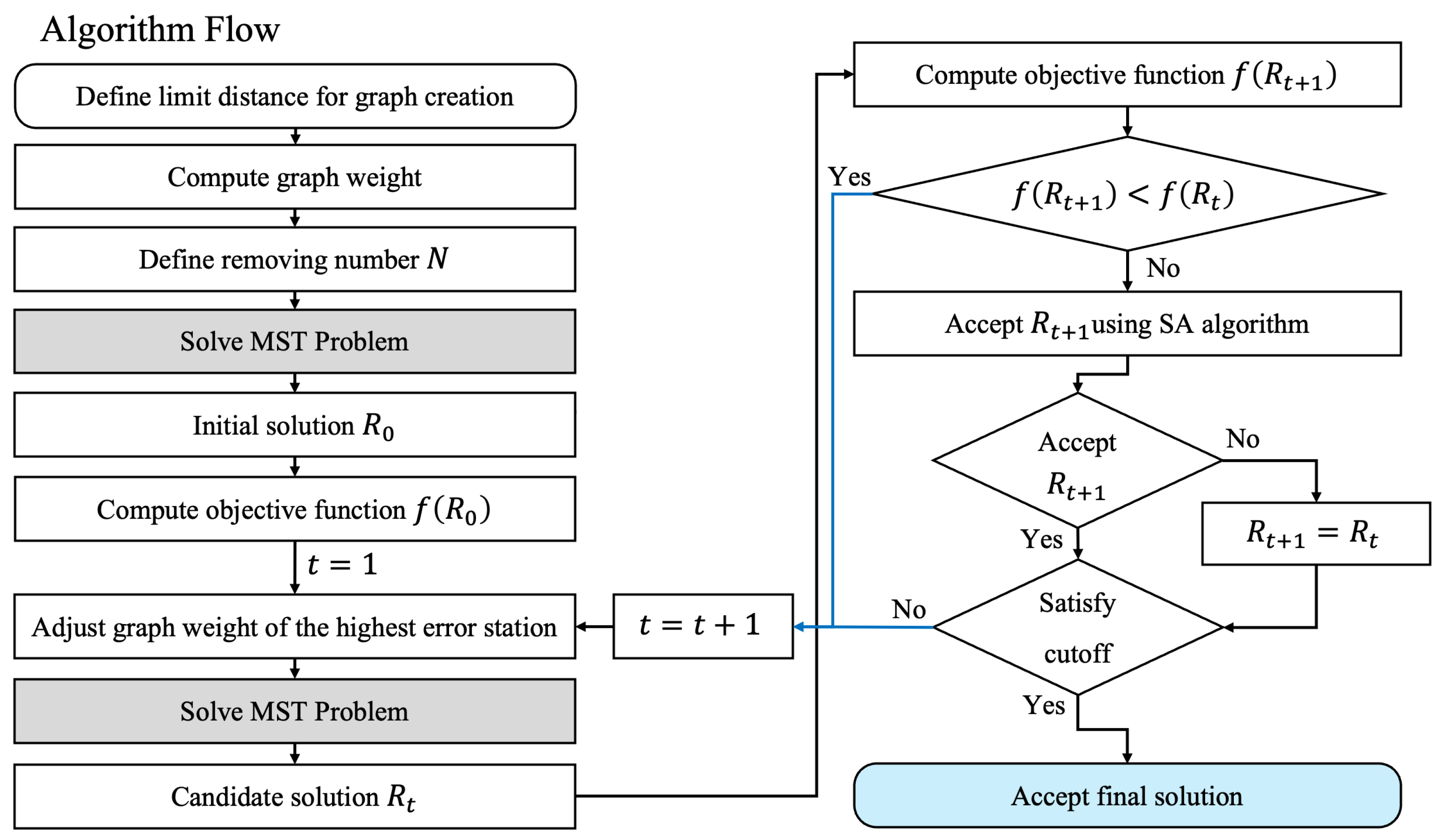
To accomplish the station selection objective, there are various stopping criteria that can be applied, such as terminating the process after obtaining the same solution for consecutive iterations, or halting the procedure after a predetermined number of repetitions. In this study, the stopping condition is based on the number of iterations. That is, the process is terminated after predefined iterations of step $t_{max}$. Algorithm 2 illustrates the workflow of the entire process for finding the optimal station selection in the network and the flowchart of Algorithm 2 is provided in Figure 3.

Algorithm 2 Hybrid MST-SA Algorithm with Adaptive Graph Weighting

Require:  Max iteration $t_{max}$, Removing number N, Cooling rate $\eta$   1: Construct an initial graph $G_0$   2: for $t=0$ to $t_{max}$ do   3:     Generate a candidate solution $R_t$ by solving system (15)–(19) with respect to $G_t$   4:     Interpolate the missing data of $R_t$ and compute $f\left(R_t\right)$   5:     if $t\ne 0$ then   6:         if $f\left(R_t\right)<f\left(R_{t-1}\right)$ then   7:            Accept the candidate solution $R_t$   8:         else   9:            Accept the candidate solution $R_t$ with probability (23) 10:            if Not accept $R_t$ then 11:                Replace $R_t$ with $R_{t-1}$ 12:            end if 13:         end if 14:         Update temperature with cooling rate in (24) 15:     end if 16:     Define the set $M_t^{*}$ corresponding to $R_t$ 17:     Assign adjusting weights to $G_{t+1}$ using (22) 18: end for 19: Obtain the final solution of removed stations $R_{t_{max}}$

5. Results

This section presents the performance of the proposed optimization method-based on two experimental scenarios. The first experiment investigates the impact of centrality applying as the edge weights of the monitoring network, while the second result shows the sensitivity of the algorithm to different cooling rates in the SA procedure. All experiments aim to minimize the AKV after the removal of selected monitoring stations. In all numerical simulations, we set the limit distance $D=50$ for preserving the connectivity of graph G and $\delta =0.8$ for the adjusting weight parameter in Equation (22). Since the $T^{*}$ in Equation (25) is $99.66$, we define the initial temperature $T_0=100$. The computational environment consisted of a system equipped with an eitgh-core CPU and 8GB of memory. Our computational analysis revealed that every five removed stations required approximately 50–70 min to complete 1000 iterations.

5.1. Effect of Centrality-Weighted Edge Adjustment

To assess the effect of centrality on the optimization process, as defined in Equation (14), the trade-off parameter $\alpha$ is varied from 0 to 1 with an increment of 0.2. With the cooling rate fixed at $\eta =0.97$, we examine the convergence of the SA optimization in achieving the local optimal AKV for specific numbers of excluded stations with $N=5,10,15,20,25$, and 30. For the purpose of clarity in presentation, six values of the parameter $\alpha$ are considered for each N, as displayed in Figure 4.

As illustrated in Figure 4a,b, the solutions converge to identical values for all $\alpha$ values when $N=5$ and 10, with $\alpha =0$ yielding the fastest convergence in both cases. One can also observe that the AKVs corresponding to $\alpha =1$, which rely solely on correlation, eventually converge to the same AKV values as those for $\alpha =0$, although they require a greater number of iterations. This suggests a difference in the efficiency of the iterative process depending on the value of $\alpha$. A similar pattern is observed for $N=25$ and 30, where $\alpha =0$ produces the lowest AKV, while other values of $\alpha$ converge to higher AKV values. For $N=15$ and $N=20$, the minimum AKV is attained at $\alpha =0.4$. These results highlight the significance of utilizing betweenness and the clustering coefficient to enhance convergence rates and local optima, rather than relying only on correlation-based weights.

5.2. Effect of Cooling Rate in SA

The cooling rate, $\eta \in [0,1]$, is a critical parameter that determines the efficiency of the algorithm. When $\eta$ approaches 1, the search process becomes more explorative, which may slow down the convergence. This occurs because SA process permits the acceptance of new candidate solutions with higher AKV values than the current one. Conversely, smaller $\eta$ values accelerate convergence but increase the risk of entrapment in local minima. In this study, cooling rates $\eta =0.8,0.9,0.95$, and $0.97$, with the last three values being suggested in [37], are selected to balance efficiency and solution quality. The results, presented in

Table 3. AKV values under different SA cooling rates $\eta$ with iteration count t at which solution convergence of case $N=30$.

$\mathit{\alpha }$	$\mathit{\eta }\mathbf{=}\mathbf{0.80}$		$\mathit{\eta }\mathbf{=}\mathbf{0.90}$		$\mathit{\eta }\mathbf{=}\mathbf{0.95}$		$\mathit{\eta }\mathbf{=}\mathbf{0.97}$
	AKV	$\mathit{t}$	AKV	$\mathit{t}$	AKV	$\mathit{t}$	AKV	$\mathit{t}$
0	68.2824	183	68.2824	200	68.2824	376	68.2824	182
0.2	73.3089	320	73.3089	361	73.3089	367	73.3089	628
0.4	73.3089	607	73.3089	609	73.3089	656	73.3089	568
0.6	73.3089	221	73.3089	307	73.3089	331	73.3089	324
0.8	73.3089	292	73.3089	351	72.9761	720	72.9761	744
1	72.7372	183	73.3089	595	73.3089	611	73.3089	733

, focus on the scenario where the number of removed monitoring stations is $N=30$, where only $\alpha =0$ converges to the optimal solution. The results compare AKV values and the number of iterations at which the AKV begins to converge, evaluated across different trade-off parameter $\alpha$ values.

One can observe that, for each $\alpha$, the AKV values are identical or very close across all cooling rates. The AKV values for $\alpha =0$ reach the local optimal solution (AKV = $68.2824$) within the maximum number of iterations. For $\alpha =0.8$, we observe that more iteration allow the process to reach better AKV values. However, this is not always the case because the SA may accept the lastest solution with higher AKV with probability. These findings suggest that larger $\eta$ in SA may give the discovery of better solutions, though at the cost of increased computational iterations.

6. Conclusions

Previous studies on optimal station network design have primarily focused on correlation-based graph methods to assess data similarity, without explicitly accounting for the underlying network structure. The main objective of this study is to incorporate centrality measures with correlation analysis within a graph-based optimization framework for monitoring network reduction. The comparative performance of correlation-based and centrality-enhanced approaches is demonstrated in the case of the rain gauge network in the northern Thailand over the period 2012–2022. The proposed method consistently attains optimal solutions with faster convergence across all scenarios compared to those obtained solely through correlation-based analysis. Notably, in cases involving the removal of 15, 20, 25, and 30 stations, only the centrality-integrated approaches achieved optimal solutions within the limited number of computational iterations. This finding underscores the importance of incorporating centrality measures, particularly as the number of removed stations increases. Furthermore, the cooling rate sensitivity analysis validates centrality integration’s importance across different algorithmic parameters. A higher cooling rate, $\eta$, typically results in a larger number of iterations for the algorithm to reach convergence. However, in certain instances, the SA method may accept suboptimal solutions during the search, which leads to the overall computational cost. This suggests that slower temperature decreases enhance the algorithm’s ability to explore broader solution space.

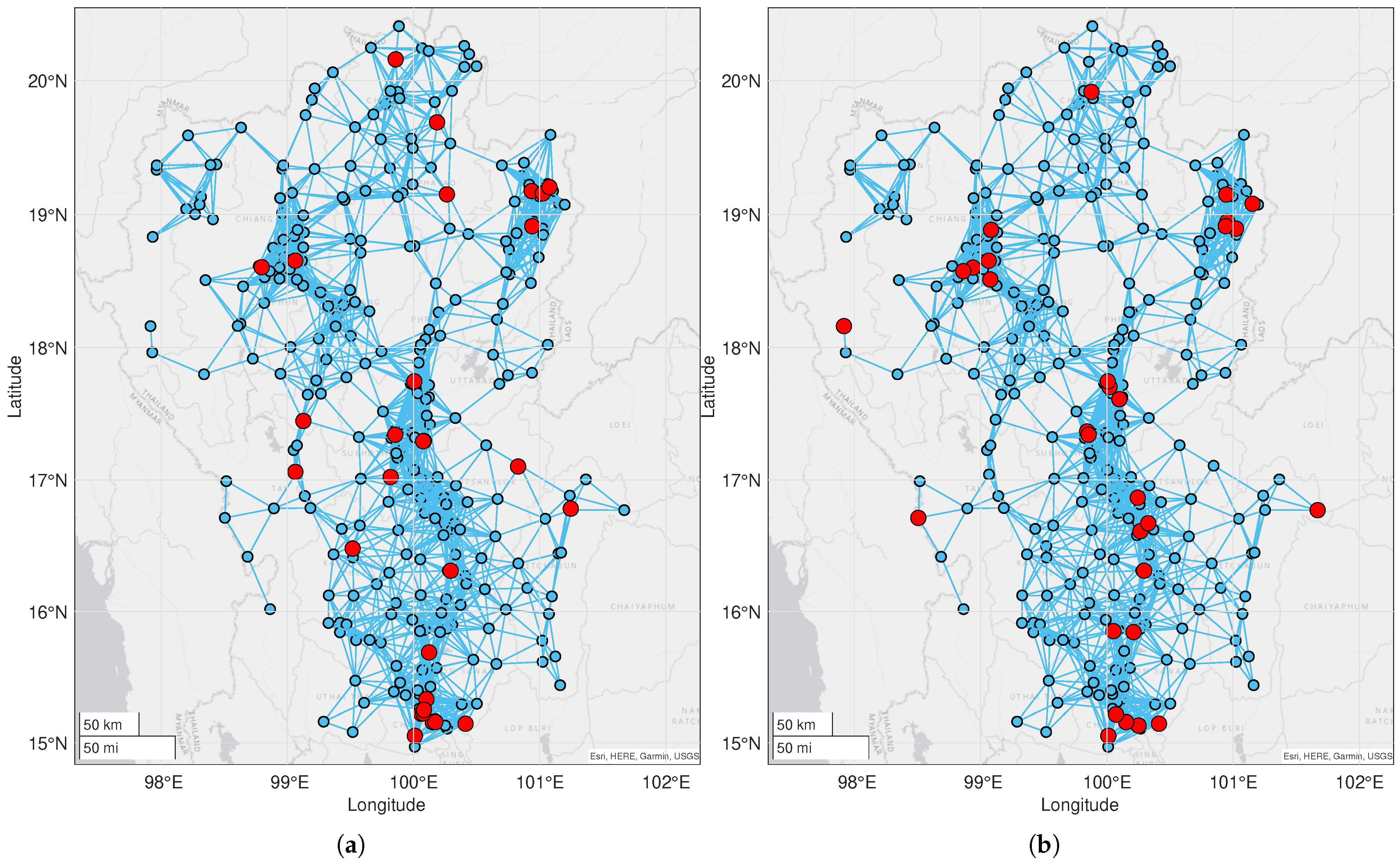
By combining betweenness centrality and clustering coefficient, the approach enables balanced node selection that offers additional structural insights into node importance within the network. At the same time, it preserves structural connectivity and ensures comprehensive spatial representation, resulting in distributed removal patterns that mitigate coverage gaps often encountered in traditional methods. The comparison in Figure 5 reveals that the centrality-integrated approach (Figure 5a) selects removal nodes distributed across the network coverage area in which it avoids the isolation of nodes within the network. In contrast, when centrality is not considered (Figure 5b), the removed stations tend to cluster in the central part of the map, with additional removals occurring at locations distant from these clusters. To ensure a well-distributed coverage of the monitoring stations across the study area, the trade-off parameter other than $\alpha =1$ should be used.

In addition to supporting cost-effective operation and maintenance, the proposed method also facilitates water resource management planning through dynamic, topology-aware scenarios for network contraction and expansion. This helps ensuring the network remains informative and connected even when stations are added or removed. Moreover, government agencies responsible for managing monitoring stations, such as the Department of Water Resources, the TMD, and the Pollution Control Department, can leverage this approach to plan and adjust monitoring networks in response to environmental changes and budgetary constraints. This approach can also enhance data connectivity and integration, enabling more effective analysis and supporting sustainable water resource management. Despite the favorable results of this study, a common limitation of hybrid approaches lies in the requirement for an optimally tuned weighting parameter. Future research should therefore explore adaptive weighting schemes, data-driven optimization algorithms, and the integration of artificial intelligence (AI) and machine learning techniques to enhance analytical capabilities and overall model performance. Extensions to dynamic networks and validation across diverse geographical and climatic contexts are also recommended to further demonstrate the practical applicability of the methodology. Additionally, more advanced kriging techniques should be explored to better match the specific characteristics of different variable types.

References

1. IPCC. IPCC Scoping Meeting on Short-Lived Climate Forcers; Institute for Global Environmental Strategies (IGES): Hayama, Japan, 2024; Available online: https://www.ipcc-nggip.iges.or.jp/public/mtdocs/pdfiles/2402_SLCF_Scoping/IPCC_SLCF_ScopingMeetingReport.pdf (accessed on 26 September 2025).
2. Nour, M.H.; Smit, D.W.; Gamal El-Din, M. Geostatistical mapping of precipitation: Implications for rain gauge network design. Water Sci. Technol. 2006, 53, 101–110. [Google Scholar] [CrossRef]
3. Cheng, K.S.; Lin, Y.C.; Liou, J.J. Rain-gauge network evaluation and augmentation using geostatistics. Hydrol. Processes Int. J. 2008, 22, 2554–2564. [Google Scholar] [CrossRef]
4. Krstanovic, P.F.; Singh, V.P. Evaluation of rainfall networks using entropy: II. Application. Water Resour. Manag. 1992, 6, 295–314. [Google Scholar] [CrossRef]
5. Yoo, C.; Jung, K.; Lee, J. Evaluation of rain gauge network using entropy theory: Comparison of mixed and continuous distribution function applications. J. Hydrol. Eng. 2008, 13, 226–235. [Google Scholar] [CrossRef]
6. Vivekanandan, N.; Jagtap, R.S. Evaluation and selection of rain gauge network using entropy. J. Inst. Eng. (India) Ser. A 2012, 93, 223–232. [Google Scholar] [CrossRef]
7. Dai, Q.; Bray, M.; Zhuo, L.; Islam, T.; Han, D. A scheme for rain gauge network design based on remotely sensed rainfall measurements. J. Hydrometeorol. 2017, 18, 363–379. [Google Scholar] [CrossRef]
8. Huang, Y.; Zhao, H.; Jiang, Y.; Lu, X. A method for the optimized design of a rain gauge network combined with satellite remote sensing data. Remote Sens. 2020, 12, 194. [Google Scholar] [CrossRef]
9. Morsy, M.; Taghizadeh-Mehrjardi, R.; Michaelides, S.; Scholten, T.; Dietrich, P.; Schmidt, K. Optimization of rain gauge networks for arid regions based on remote sensing data. Remote Sens. 2021, 13, 4243. [Google Scholar] [CrossRef]
10. Erdélyi, D.; Hatvani, I.G.; Jeon, H.; Jones, M.; Tyler, J.; Kern, Z. Predicting spatial distribution of stable isotopes in precipitation by classical geostatistical-and machine learning methods. J. Hydrol. 2023, 617, 129129. [Google Scholar] [CrossRef]
11. Kassim, A.H.M.; Kottegoda, N.T. Rainfall network design through comparative kriging methods. Hydrol. Sci. J. 1991, 36, 223–240. [Google Scholar] [CrossRef]
12. Adhikary, S.K.; Yilmaz, A.G.; Muttil, N. Optimal design of rain gauge network in the Middle Yarra River catchment, Australia. Hydrol. Processes 2015, 29, 2582–2599. [Google Scholar] [CrossRef]
13. Adhikary, S.K.; Muttil, N.; Yilmaz, A.G. Cokriging for enhanced spatial interpolation of rainfall in two Australian catchments. Hydrol. Processes 2017, 31, 2143–2161. [Google Scholar] [CrossRef]
14. Aziz, M.K.B.M.; Yusof, F.; Daud, Z.M.; Yusop, Z.; Kasno, M.A. Optimal design of rain gauge network in Johor by using geostatistics and particle swarm optimization. Geomate J. 2016, 11, 2422–2428. [Google Scholar]
15. Attar, M.; Abedini, M.J.; Akbari, R. Optimal prioritization of rain gauge stations for areal estimation of annual rainfall via coupling geostatistics with artificial bee colony optimization. J. Spat. Sci. 2019, 64, 257–274. [Google Scholar] [CrossRef]
16. Bayat, B.; Hosseini, K.; Nasseri, M.; Karami, H. Challenge of rainfall network design considering spatial versus spatiotemporal variations. J. Hydrol. 2019, 574, 990–1002. [Google Scholar] [CrossRef]
17. Pardo-Igúzquiza, E. Optimal selection of number and location of rainfall gauges for areal rainfall estimation using geostatistics and simulated annealing. J. Hydrol. 1998, 210, 206–220. [Google Scholar] [CrossRef]
18. Wadoux, A.M.C.; Brus, D.J.; Rico-Ramirez, M.A.; Heuvelink, G.B. Sampling design optimisation for rainfall prediction using a non-stationary geostatistical model. Adv. Water Resour. 2017, 107, 126–138. [Google Scholar] [CrossRef]
19. Omer, T.; Hassan, M.U.; Hussain, I.; Ilyas, M.; Hashmi, S.G.M.D.; Khan, Y.A. Optimization of monitoring network to the rainfall distribution by using stochastic search algorithms: Lesson from Pakistan. Tellus A Dyn. Meteorol. Oceanogr. 2022, 74, 333–345. [Google Scholar] [CrossRef]
20. Donges, J.F.; Schultz, H.C.; Marwan, N.; Zou, Y.; Kurths, J. Investigating the topology of interacting networks: Theory and application to coupled climate subnetworks. Eur. Phys. J. B 2011, 84, 635–651. [Google Scholar] [CrossRef]
21. Scarsoglio, S.; Laio, F.; Ridolfi, L. Climate dynamics: A network-based approach for the analysis of global precipitation. PLoS ONE 2013, 8, e71129. [Google Scholar] [CrossRef]
22. Ebert-Uphoff, I.; Deng, Y. Causal discovery for climate research using graphical models. J. Clim. 2012, 25, 5648–5665. [Google Scholar] [CrossRef]
23. Hlinka, J.; Hartman, D.; Jajcay, N.; Tomeček, D.; Tintěra, J.; Paluš, M. Small-world bias of correlation networks: From brain to climate. Chaos Interdiscip. J. Nonlinear Sci. 2017, 27, 035812. [Google Scholar] [CrossRef]
24. Sukharev, J.; Wang, C.; Ma, K.L.; Wittenberg, A.T. Correlation study of time-varying multivariate climate data sets. In Proceedings of the 2009 IEEE Pacific Visualization Symposium, Beijing, China, 20–23 April 2009; pp. 161–168. [Google Scholar]
25. Takahashi, H.G.; Yasunari, T. Decreasing trend in rainfall over Indochina during the late summer monsoon: Impact of tropical cyclones. J. Meteorol. Soc. Jpn. Ser. II 2008, 86, 429–438. [Google Scholar] [CrossRef]
26. Zhang, P.; Chartrand, G. Introduction to Graph Theory; Tata McGraw-Hill: New York, NY, USA, 2006; Volume 2, No. 2.1. [Google Scholar]
27. Ariyoshi, H. Cut-set graph and systematic generation of separating sets. IEEE Trans. Circuit Theory 2003, 19, 233–240. [Google Scholar] [CrossRef]
28. Watts, D.J.; Strogatz, S.H. Collective dynamics of ‘small-world’networks. Nature 1998, 393, 440–442. [Google Scholar] [CrossRef]
29. Freeman, L.C. A set of measures of centrality based on betweenness. Sociometry 1977, 40, 35–41. [Google Scholar] [CrossRef]
30. Beineke, L.W.; Bagga, J.S. Line Graphs and Line Digraphs; Springer: Cham, Switzerland, 2021. [Google Scholar]
31. Cressie, N. Spatial prediction and ordinary kriging. Math. Geol. 1988, 20, 405–421. [Google Scholar] [CrossRef]
32. Matheron, G. Principles of geosatistics. Econ. Geol. 1963, 58, 1246–1266. [Google Scholar] [CrossRef]
33. Kirkpatrick, S.; Gelatt, C.D., Jr.; Vecchi, M.P. Optimization by simulated annealing. Science 1983, 220, 671–680. [Google Scholar] [CrossRef] [PubMed]
34. Černý, V. Thermodynamical approach to the traveling salesman problem: An efficient simulation algorithm. J. Optim. Theory Appl. 1985, 45, 41–51. [Google Scholar] [CrossRef]
35. Sedgwick, P. Pearson’s correlation coefficient. BMJ 2012, 345, e4483. [Google Scholar] [CrossRef]
36. Ben-Ameur, W. Computing the initial temperature of simulated annealing. Comput. Optim. Appl. 2004, 29, 369–385. [Google Scholar] [CrossRef]
37. Amorim, A.M.; Gonçalves, A.B.; Nunes, L.M.; Sousa, A.J. Optimizing the location of weather monitoring stations using estimation uncertainty. Int. J. Climatol. 2012, 32, 941–952. [Google Scholar] [CrossRef]
Figure 1. (a) Northern Thailand area height above sea level. (b) Current 317 monitoring stations’ locations (blue nodes) in the Northern Thailand.
Mathematics 13 03421 g001
Figure 2. Connected graph of monitoring stations (blue nodes) with an edge distance limit of 48.2175 km.
Mathematics 13 03421 g002
Figure 3. Flowchart of Algorithm 2 for removing redundant stations.
Mathematics 13 03421 g003
Figure 4. Iterative AKV in node removal process for monitoring networks with (a) 5 stations, (b) 10 stations, (c) 15 stations, (d) 20 stations, (e) 25 stations, and (f) 30 stations.
Mathematics 13 03421 g004
Figure 5. Spatial distribution of the remaining stations (blue nodes) with 30 removed stations (red nodes) at η = 0.80 for different values of trade-off parameter α (a) centrality-integrated case, α = 0.5 , and (b) no-centrality case, α = 1 .
Mathematics 13 03421 g005