A Hybrid TLBO-Cheetah Algorithm for Multi-Objective Optimization of SOP-Integrated Distribution Networks
Abstract
1. Introduction
- One of the major issues in the field is the premature convergence problem of metaheuristic algorithms in the high-dimensional, non-convex search space. The proposed hTLBO–CO introduces a critical architectural novelty through its parallel cooperative architecture. Unlike sequential hybrids, this approach enables concurrent execution of specialized search phases—TLBO for exploitation [27], CO for exploration [28], and a social learning phase—supported by a collaborative knowledge repository. This arrangement enables continuous, bidirectional information sharing and dynamic resource pooling, effectively resolving premature convergence and stagnation issues affecting other solvers.
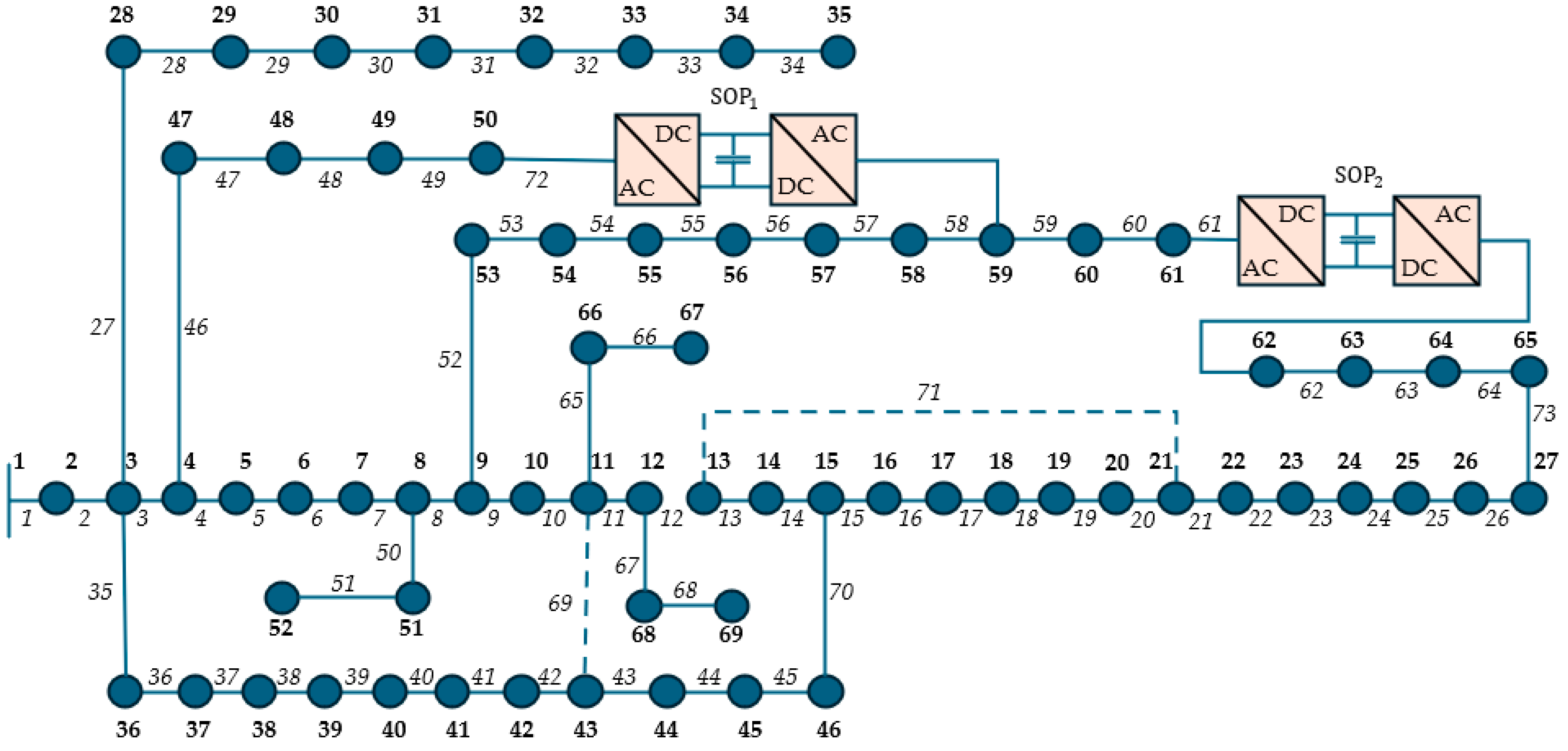
- The existing models are likely to lack effectiveness in modeling the realistic integration of SOPs. The new formulation takes a significant step by allowing the adaptive placement of SOPs on a wider range of network switches, thereby expanding the network of feasible solutions. A principal innovation is the introduction of a new topological compatibility constraint, one that systematically captures the important physical requirement that an SOP must be installed in an open branch. This ensures that all solutions derived are topologically correct and physically viable, which counteracts the prevalent source of infeasibility in other approaches.
- Moving beyond standard single-objective optimization, this work introduces an entire multi-objective analysis that precisely quantifies the trade-offs between key performance metrics, such as power loss, voltage profile, and capital expenditure. This offers system planners a robust decision-making framework. Moreover, the demonstrated performance excellence is tightly supported by extensive statistical testing and provides high confidence in the algorithm’s robustness and reliability across various independent runs.
- Computational intractability of the underlying problem for large-scale networks is a main practical hindrance. The design of the framework involves an evolved multi-stage approach to dealing with sophisticated constraints and computational acceleration algorithms. This integrated solution confronts the scalability challenge head-on, enabling efficient optimization of realistically scaled distribution networks, where conventional methods typically become ineffective or fail.
- A novel hTLBO–CO hybrid algorithm with a parallel cooperative design.
- A comprehensive mathematical model with an innovative topological compatibility constraint.
- A robust constraint-handling and computational strategy for scalability.
- Extensive validation, such as multi-objective Pareto analysis and statistical significance testing, to demonstrate consistent supremacy.
2. Mathematical Formulation of SOP-Integrated Network Reconfiguration
2.1. Objective Function
2.2. Decision Vector Construction
2.3. Constraints
2.3.1. SOP Operational Constraints
2.3.2. Voltage Constraints
2.3.3. Topological Constraints
2.3.4. Switch Status Constraints
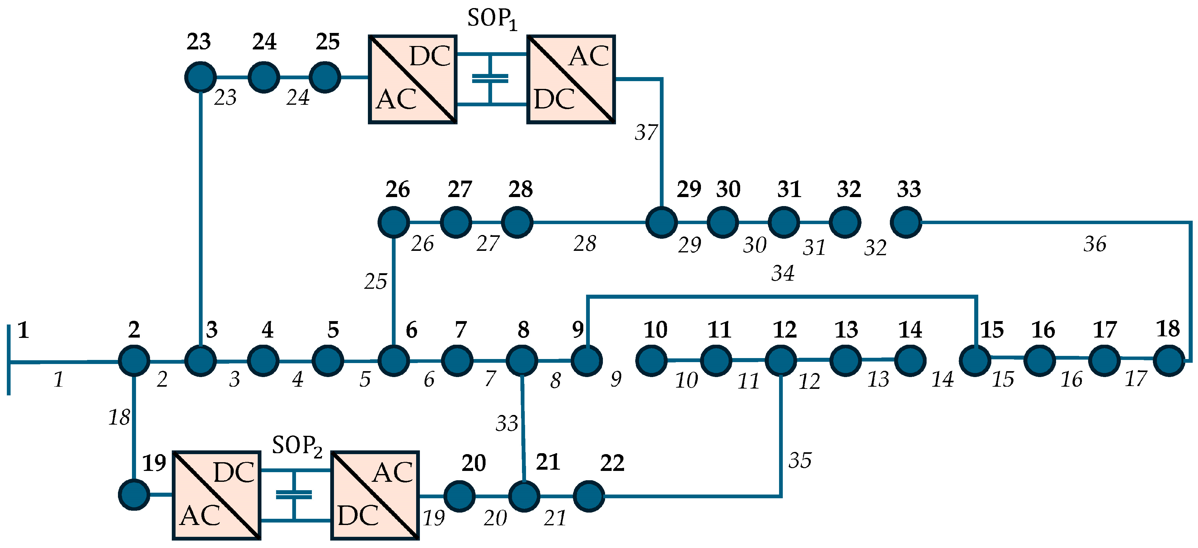
2.3.5. SOP Installation Constraints
2.3.6. Topological Compatibility
2.4. Solution Space Characterization
- A combinatorial component with possible configurations;
- A continuous component, forming a -dimensional polytope bounded by the SOP capacity constraints.
2.5. Computational Complexity Analysis
3. Proposed Hybrid TLBO-CO Algorithm
3.1. Algorithm Overview
3.2. Population Initialization and Management
3.3. TLBO Teacher Phase (Focused Exploitation)
3.4. CO Hunting Phase (Intelligent Exploration)
3.5. TLBO Learner Phase (Social Learning)
3.6. Constraint Handling
- Boundary Correction: Values out of variable bounds are set through component-wise clamping:
- Feasibility Projection: Infeasible solutions of nonlinear constraints are projected onto the set of feasible solutions byThis is accomplished through an efficient active-set method.
- Lexicographic Selection: A feasibility-first rule is imposed during selection, ensuring that the algorithm always prefers and converges towards feasible regions.
3.7. Computational Complexity
3.8. Convergence Analysis
- It provides the global best solution that guides the update equations in both the Teacher Phase (Equation (18)) and the CO’s pursuit mode (Equation (21));
- It serves as a source for re-injecting high-quality, diverse solutions back into the sub-populations, preventing stagnation and fostering cooperative learning.
| Algorithm 1: Pseudocode of the hTLBO-CO algorithm |
| Input: Population Size N, Max Iterations tmax, Lower Bounds lb, Upper Bounds ub Output: Best solution Xbest 1: Initialize population P of size N using Equation (14)//Section 3.2 2: Evaluate fitness f(X) for all individuals X ∈ P 3: Xbest ← argmin_{X ∈ P} f(X) 4: for iteration t = 1 to tmax do 5: Partition P into P1, P2, P3 using ratios from Equation (15)//Section 3.2 6: 7: % Phase 1: TLBO Teacher Phase (P1- Exploitation) 8: for each individual in sub-population P1 do 9: Calculate adaptive TF (Equation (16)) 10: Calculate fitness-weighted mean (Equation (17)) 11: Update solution: ← Apply Equation (18) 12: Enforce constraints on (Section 3.6) 13: Evaluate f() and update if improved 14: end for 15: 16: % Phase 2: CO Hunting Phase (P2- Exploration) 17: Calculate current survey probability (Equation (22)) 18: for each individual in sub-population P2 do 19: if rand() < then 20: Update via Survey Mode: ← Apply Equations (19) and (20) 21: else 22: Update via Pursuit Mode: ← Apply Equation. (21) 23: end if 24: Enforce constraints on (Section 3.6) 25: Evaluate f() and update if improved 26: end for 27: 28: % Phase 3: TLBO Learner Phase (P3—Social Learning) 29: Calculate current learning rate r (Equation (23)) 30: for each individual in sub-population P3 do 31: Randomly select a partner from P (j ≠ i) via tournament selection 32: Update solution: ← Apply Equation (24) 33: Enforce constraints on (Section 3.6) 34: Evaluate f() and update if improved 35: end for 36: 37: Update the best global solution: Xbest ← argmin(f(Xbest), min_{X ∈ P} f(X)) 38: Update moving averages , , and for adaptive ratios (Equation (15)) 39: end for 40: Return Xbest |
4. Implementation Framework for SOP-Integrated Reconfiguration
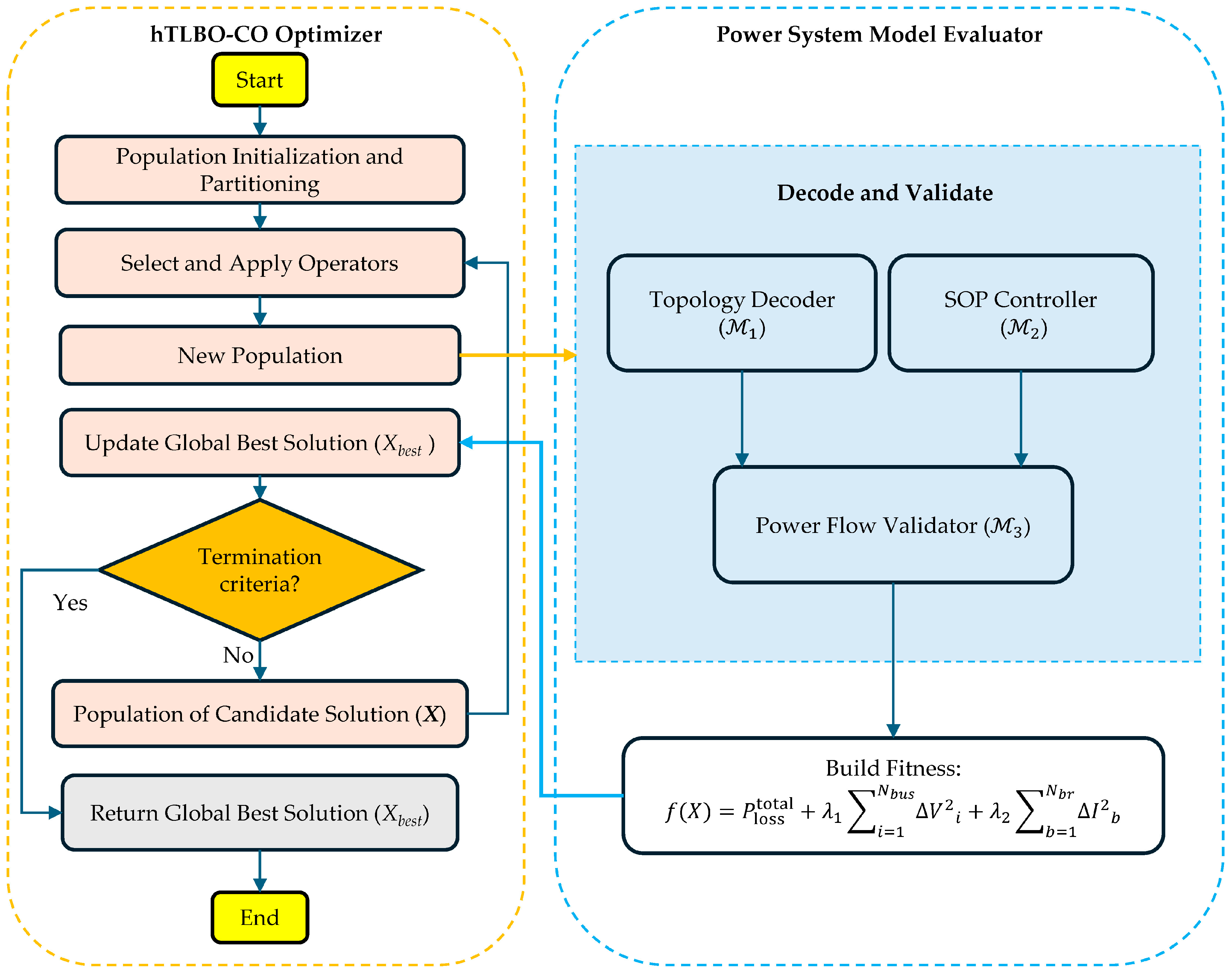
4.1. Algorithmic Integration with Power System Model
- Topology Decoder (): This module translates the binary part of the decision vector X (switch state and SOP placement flags ) to a valid radial network topology. This module constructs the network graph associated with iteration t with primitives of graph theory:Here, is the set of buses (nodes) and is the set of energized branches (edges) determined by the closed switches.
- SOP Controller (): This module is responsible for the continuous part of X, which computes the active and reactive power setpoints () of every installed SOP. It also ensures the setpoints are within the operating envelope of the device prior to presenting them to the power flow solver.
- Power Flow Validator (): This is the principal computational engine that assesses the efficiency and feasibility of a possible solution. It calculates the power flow equations of the topology input provided from with the SOP injections from to determine the bus voltages, branch flows, and total power loss. It also checks for constraint violations.
4.2. Solution Representation and Initialization
- Switch States (): Initialized via a Bernoulli distribution, , to randomly generate radial configurations.
- SOP Placement (): Set with an initially biased Bernoulli distribution, , to encourage diversity while being respectful of the constraints.
- SOP Power Setpoints (): Initialized with a uniform distribution within their operational limits, .
4.3. Constraint Handling Mechanism
- Topological Feasibility: Radiality constraints are enforced throughwhere A represents the incidence matrix. If a solution violates radiality, then a repair mechanism is initiated with the help of an MST algorithm:The MST uses branch resistances as edge weights to compute the radial topology with the least possible resist losses while preserving connectivity, restoring the solution.
- SOP-Placement Coupling: The logical constraint (meaning an SOP can only be placed onto an open branch) is enforced directly in the following solution representation:This basic projection guarantees feasibility without substantially altering the optimizer’s direction of search.
- Power Flow and Device Constraints: The power flow checker checks violations of voltage constraints () and branch current constraints (). SOP capacity constraints are enforced via a direct projection of their power setpoints onto the feasible circle defined by :
- Penalty Function: Infeasible solutions corresponding to violation of the soft constraints (e.g., voltage limit violations) are penalized but not eliminated to steer the search towards feasible regions again. The fitness function becomeswhere and are the magnitudes of voltage and current limit violations, respectively, and and are large penalty coefficients.
4.4. Fitness Evaluation Pipeline
- Topology Validation and Repair: The switch states are decoded to a graph . If non-radial, then MST repair is applied.
- SOP Activation: The power injections corresponding to every unplaced SOP () are initialized to zero.
- Power Flow Solution: A balanced three-phase power flow is solved using a current injection method, which is also effective for radial distribution networks.
- Loss Computation: The overall power loss is determined from branch flows.
- Application of Penalty: All remaining constraint violations’ penalty terms are added to the loss value to obtain the final fitness .
4.5. Solution Evaluation and Iterative Convergence
4.6. Computational Acceleration Techniques
- Topology Catching: Radiality status and power flow outcomes of frequent switch configurations are saved in a hash-map to avoid redundant calculation.
- Warm Starts: The power flow solver is initialized with the last evaluation’s corresponding topology voltage profile, significantly reducing the number of iterations required to converge.
- Parallel Assessment: The assessment of the fitness of the population is divided across many CPU cores since these assessments do not occur sequentially but are independent of each other. This leads to almost linear speedup with the number of cores present.
4.7. Convergence Monitoring
- Centroid Motion (): Assesses the swarm’s center of mass movement over an iteration window to check if the swarm is still exploring.
- Population Diversity (): Calculates the rank of the covariance matrix of the population, scaled by the dimension D. A low value indicates convergence and loss of diversity.
- Improvement Rate (): Relative improvement of the best global solution during a window of iterations.
5. Simulation Results and Discussion
5.1. Experimental Setup
5.2. Parameter Sensitivity Analysis
5.3. Results for the IEEE 33-Bus Test System
5.4. Results for the IEEE 69-Bus Test System
5.5. 119-Bus Large-Scale Test System
5.6. Convergence Analysis and Algorithmic Stability
5.7. Statistical Analysis and Computational Efficiency
5.8. Multi-Objective Analysis and Pareto Front Evaluation
5.9. Comparison with State-of-the-Art
5.10. Discussion of Challenges
6. Conclusions
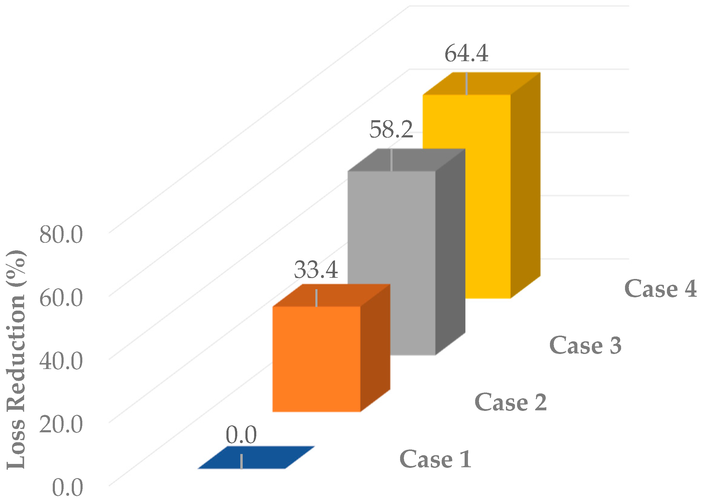
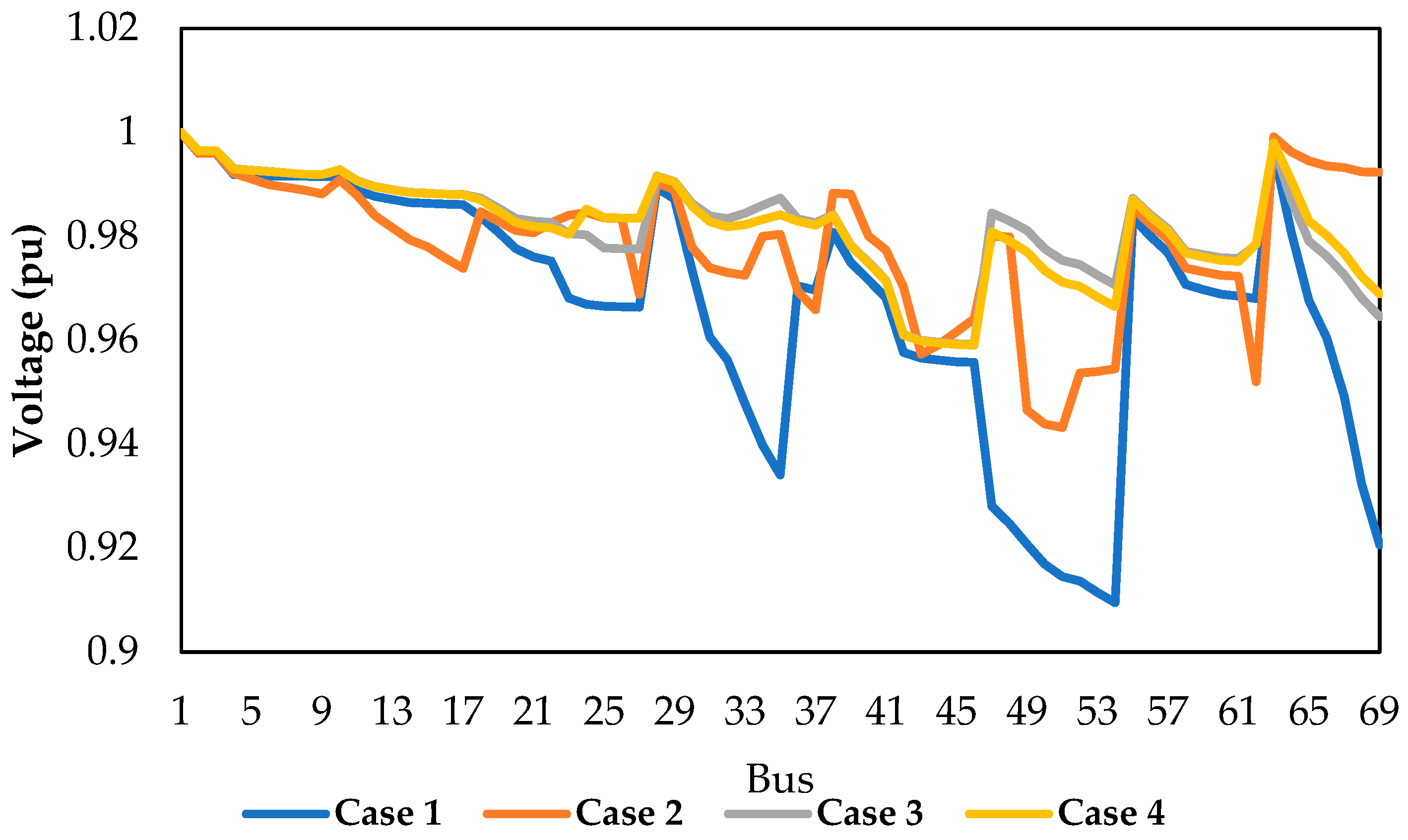
- The proposed hTLBO-CO on the IEEE 33-bus network led to a total loss of 74.14 kW for the collaborative DNR-SOP optimization scenario, a 64.44% improvement over the base case and a winning outcome against all opponents.
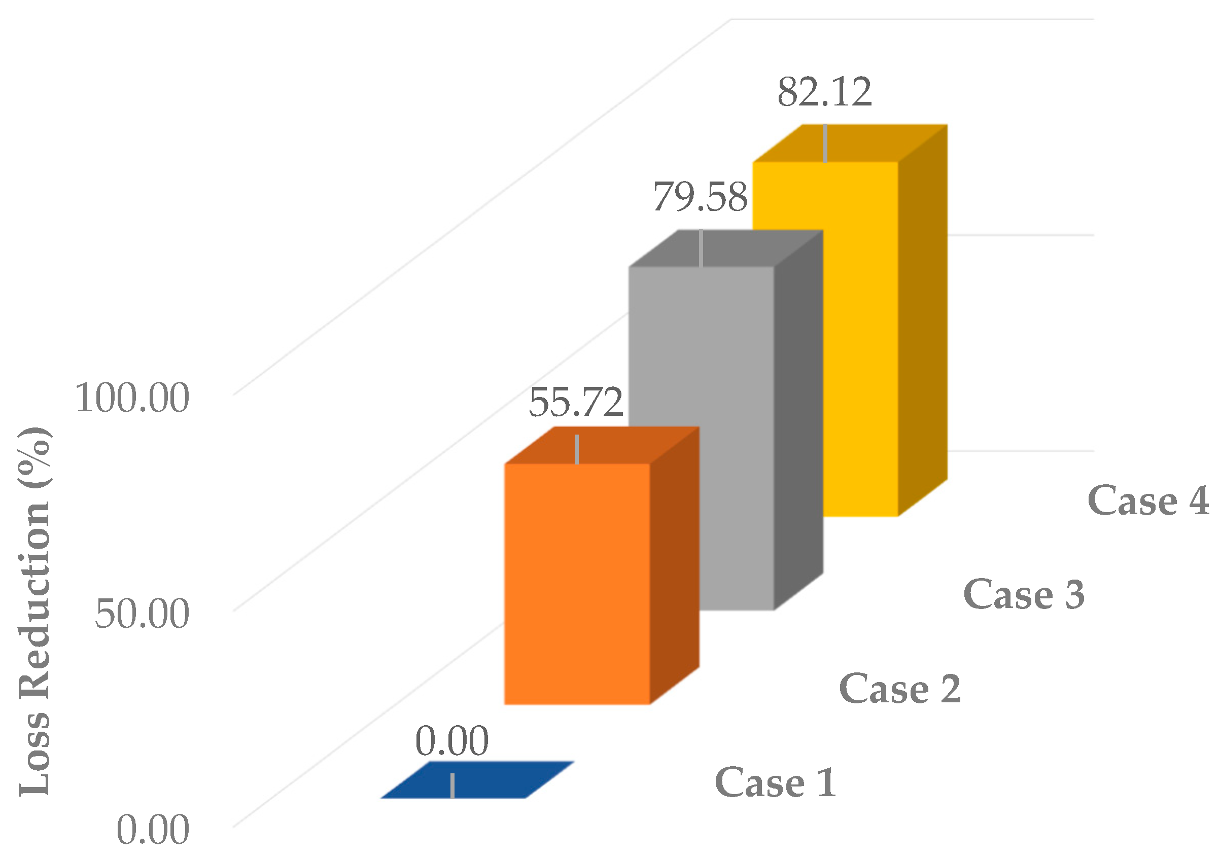
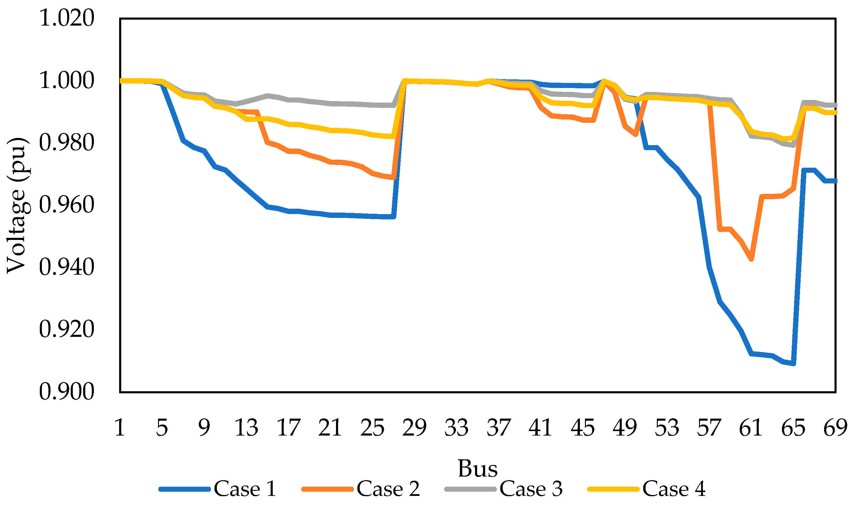
- For the expanded IEEE 69-bus system, losses reduced further to 40.23 kW for the joint optimization case, an impressive 82.12% improvement.
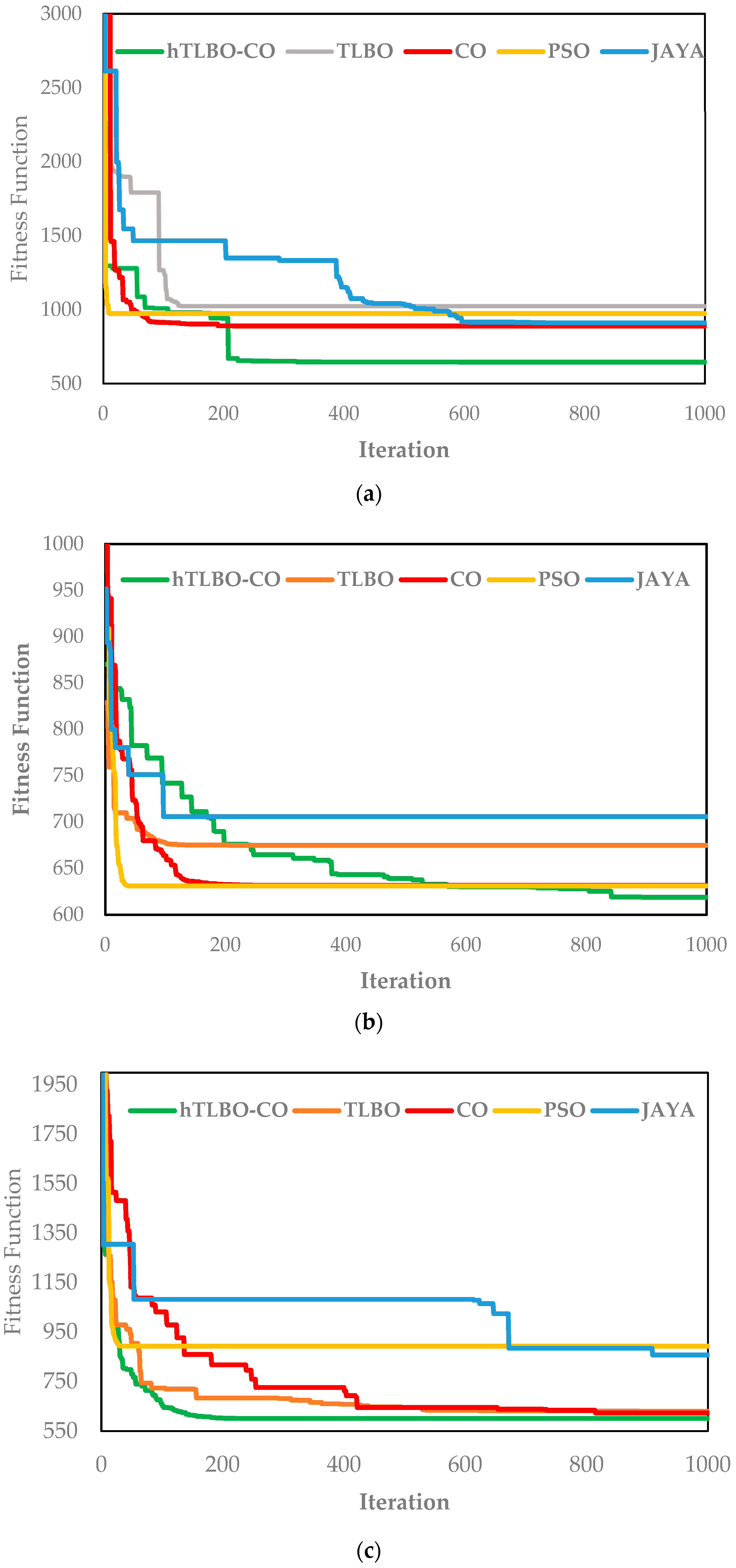
- Remarkably, on the large-scale 119-bus system—a test case for scalability—the hTLBO-CO performed outstandingly. In the reconfiguration-only scenario, it cut loss by 50.30% (645.09 kW), surpassing the ARO algorithm’s best-reported solution of 34.36% reduction by more than 15 percentage points. This result, from a new switching configuration, demonstrates the algorithm’s strongest exploration capability in big combinatorial spaces.
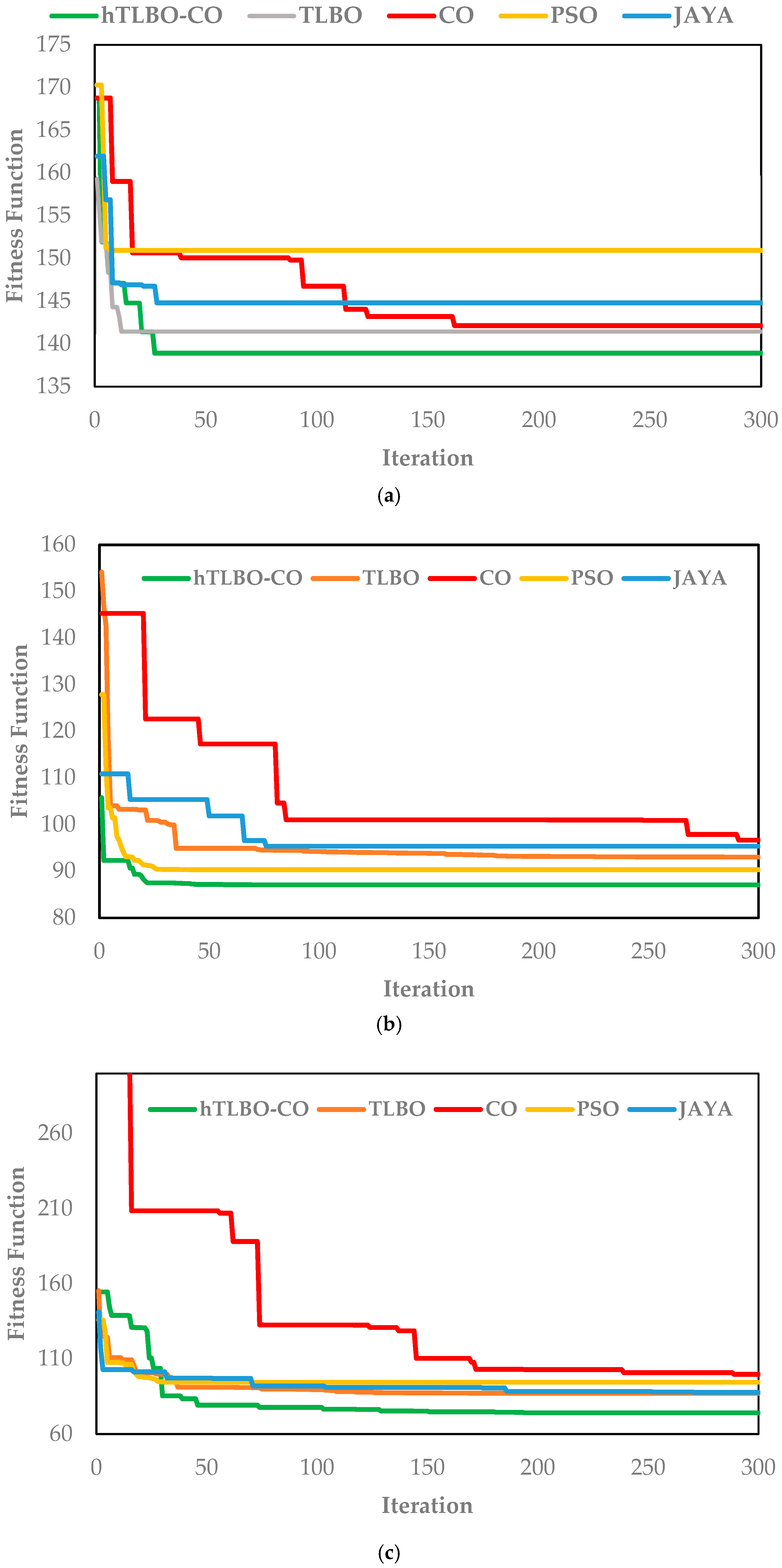
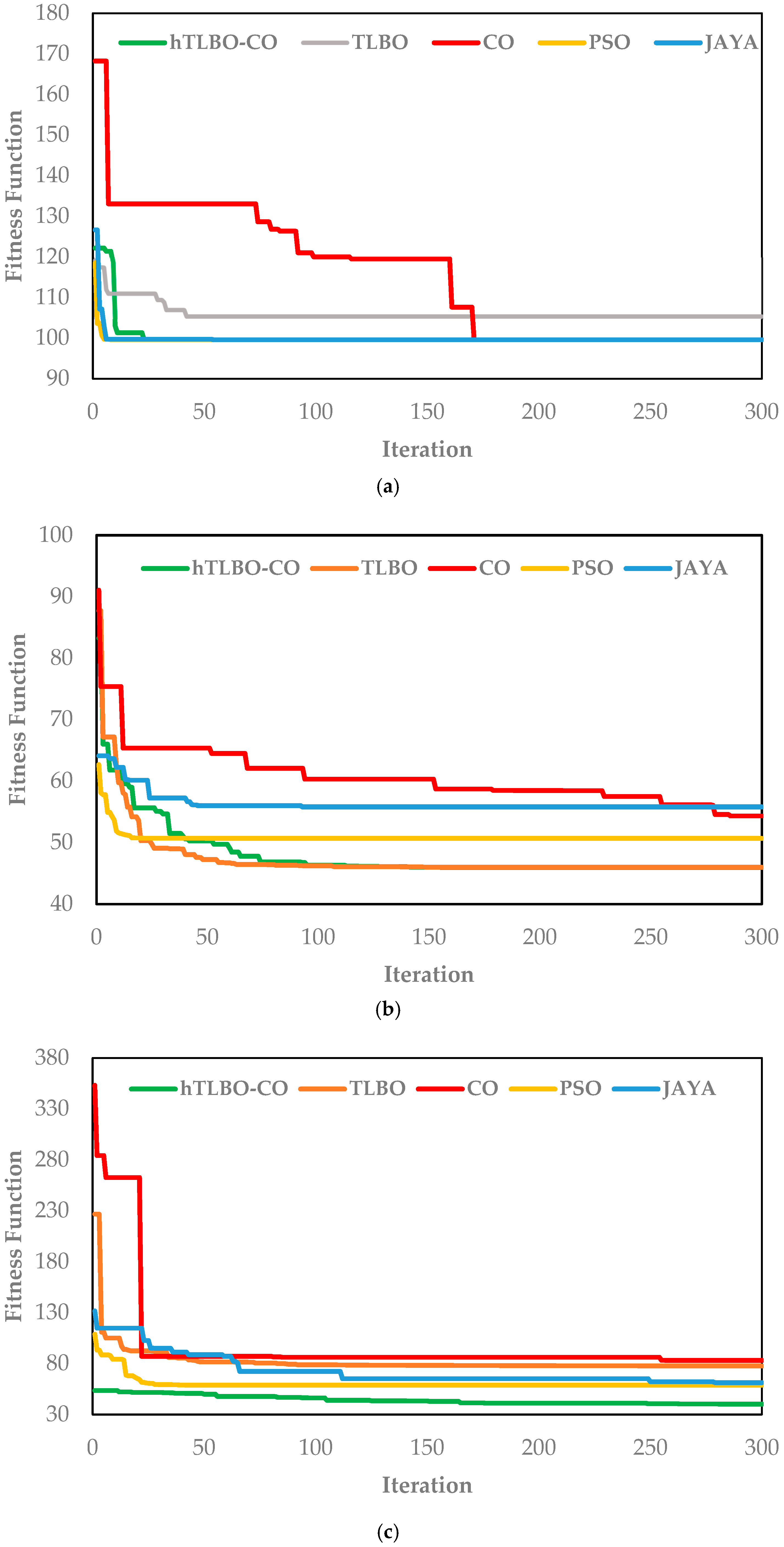
- A tight convergence analysis revealed that hTLBO-CO achieved 99% of the ultimate solution much faster and more reliably than competitors, with very minimal final-phase fluctuation (e.g., <0.05% for the 33-bus system), which speaks to its algorithmic efficiency and stability.
- Detailed statistical tests, including Friedman and Wilcoxon signed-rank tests, consistently confirmed the dominance of hTLBO-CO with near-zero p-values (p < 0.05), indicating that its performance improvements are statistically significant and not by random chance.
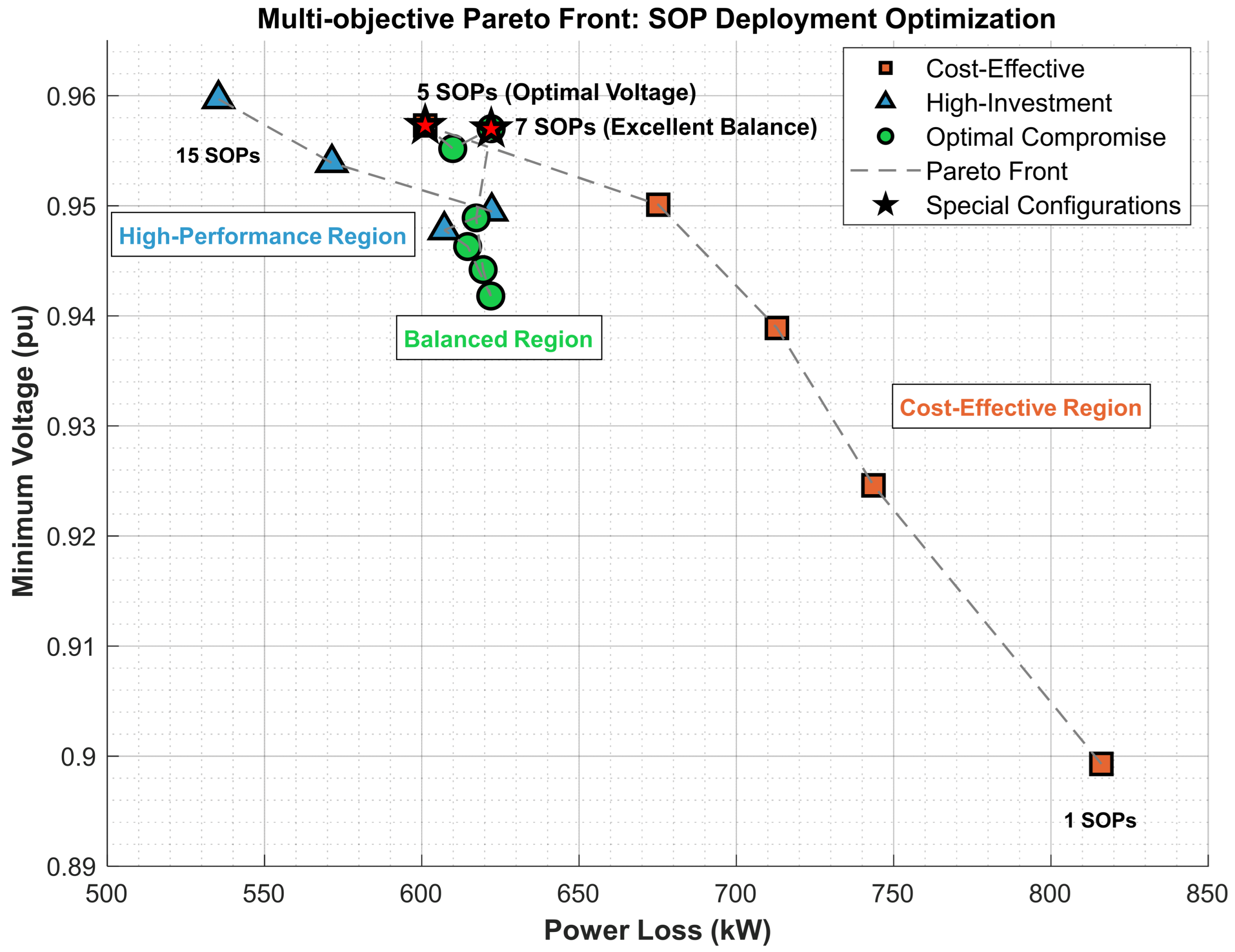
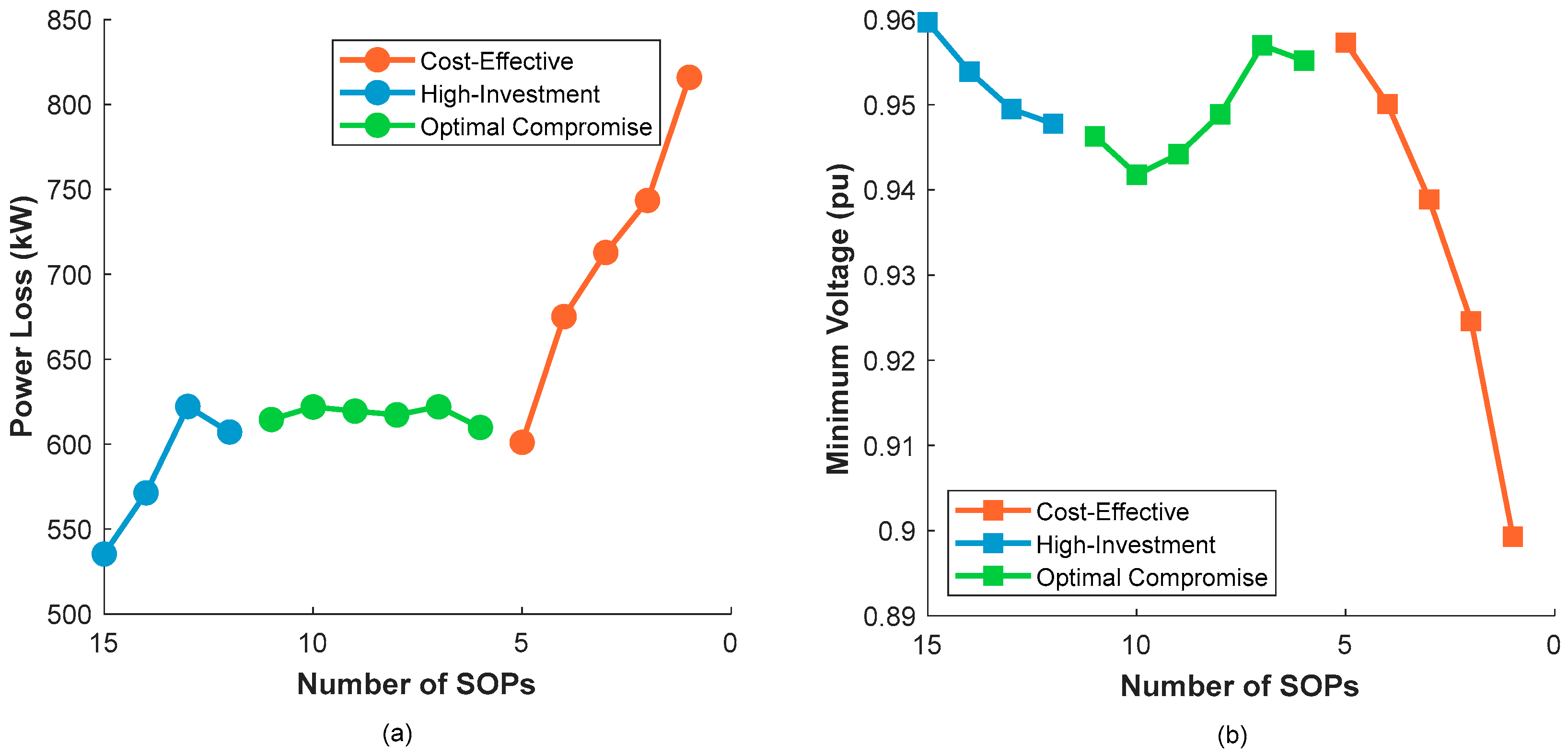
- The Pareto front analysis of the 119-bus system provides system planners with a clear, quantitative trade-off between performance and cost. It identifies strategic zones of compromise, such as the 5-SOP scheme that provided the best voltage profile (0.9573 p.u.) with highly competitive power losses (601.10 kW), providing a data-driven foundation for cost-effective investment planning.
Author Contributions
Funding
Data Availability Statement
Acknowledgments
Conflicts of Interest
References
- Jayabarathi, T.; Raghunathan, T.; Mithulananthan, N.; Cherukuri, S.H.C.; Sai, G.L. Enhancement of Distribution System Performance with Reconfiguration, Distributed Generation and Capacitor Bank Deployment. Heliyon 2024, 10, e26343. [Google Scholar] [CrossRef] [PubMed]
- Sambaiah, K.S.; Jayabarathi, T. Optimal Reconfiguration of Distribution Network in Presence of D-STATCOM and Photovoltaic Array Using a Metaheuristic Algorithm. Eur. J. Electr. Eng. Comput. Sci. 2020, 4. [Google Scholar] [CrossRef]
- Haggar, M.F.A.; Beshr, E.; Eteiba, M.B. Minimizing Power Loss in Distribution System by Optimal Sizing and Sitting of Distributed Generators with Network Reconfiguration Using Grey Wolf and Particle Swarm Optimizers. In Proceedings of the 2018 IEEE International Conference on Environment and Electrical Engineering and 2018 IEEE Industrial and Commercial Power Systems Europe (EEEIC/I&CPS Europe), Palermo, Italy, 12–15 June 2018; pp. 1–6. [Google Scholar]
- Adetunji, K.; Hofsajer, I.; Cheng, L. Trends in the Optimal Location and Sizing of Electrical Units in Smart Grids Using Meta-Heuristic Algorithms. arXiv 2019, arXiv:1910.09312. [Google Scholar]
- Jordehi, A.R. DG Allocation and Reconfiguration in Distribution Systems by Metaheuristic Optimisation Algorithms: A Comparative Analysis. In Proceedings of the 2018 IEEE PES Innovative Smart Grid Technologies Conference Europe (ISGT-Europe), Sarajevo, Bosnia and Herzegovina, 21–25 October 2018; pp. 1–6. [Google Scholar]
- HassanzadehFard, H.; Jalilian, A. A Novel Objective Function for Optimal DG Allocation in Distribution Systems Using Meta-Heuristic Algorithms. Int. J. Green Energy 2016, 13, 1615–1625. [Google Scholar] [CrossRef]
- Quintero-Duran, M.; Candelo, J.E.; Sousa, V. Recent Trends of the Most Used Metaheuristic Techniques for Distribution Network Reconfiguration. J. Eng. Sci. Technol. Rev. 2017, 10, 159–173. [Google Scholar] [CrossRef]
- Divya, M.; Bindu, R. Ant Colony Optimization Method Applied to Distribution Network Reconfiguration. Int. J. Adv. Res. Comput. Commun. Eng. 2013, 2, 3817–3824. [Google Scholar]
- Kouzou, A.; Mohammedi, R.D. Optimal Reconfiguration of a Radial Power Distribution Network Based on Meta-Heuristic Optimization Algorithms. In Proceedings of the 2015 4th International Conference on Electric Power and Energy Conversion Systems (EPECS), Sharjah, United Arab Emirates, 24–26 November 2015; pp. 1–6. [Google Scholar]
- Helmi, A.M.; Carli, R.; Dotoli, M.; Ramadan, H.S. Efficient and Sustainable Reconfiguration of Distribution Networks via Metaheuristic Optimization. IEEE Trans. Autom. Sci. Eng. 2021, 19, 82–98. [Google Scholar] [CrossRef]
- Cikan, M.; Kekezoglu, B. Comparison of Metaheuristic Optimization Techniques Including Equilibrium Optimizer Algorithm in Power Distribution Network Reconfiguration. Alex. Eng. J. 2022, 61, 991–1031. [Google Scholar] [CrossRef]
- Kamel, S.; Hamour, H.; Ahmed, M.H.; Nasrat, L. Atom Search Optimization Algorithm for Optimal Radial Distribution System Reconfiguration. In Proceedings of the 2019 International Conference on Computer, Control, Electrical, and Electronics Engineering (ICCCEEE), Khartoum, Sudan, 21–23 September 2019; pp. 1–5. [Google Scholar]
- Tatipally, S.; Ankeshwarapu, S.; Maheswarapu, S. Swarm Intelligence Methods for Optimal Network Reconfiguration of Distribution System. In Proceedings of the 2022 IEEE International Power and Renewable Energy Conference (IPRECON), Kollam, India, 16–18 December 2022; pp. 1–6. [Google Scholar]
- Ahanch, M.; Asasi, M.S.; Amiri, M.S. A Grasshopper Optimization Algorithm to Solve Optimal Distribution System Reconfiguration and Distributed Generation Placement Problem. In Proceedings of the 2017 IEEE 4th International Conference on Knowledge-Based Engineering and Innovation (KBEI), Kollam, India, 16–18 December 2017; pp. 659–666. [Google Scholar]
- Gomes, Y.R.; Belati, E.A.; Vargas, R. Flower Pollination Algorithm for Distribution System Reconfiguration Problem. In Proceedings of the 2021 IEEE PES Innovative Smart Grid Technologies Conference-Latin America (ISGT Latin America), Lima, Peru, 15–17 September 2021; pp. 1–5. [Google Scholar]
- Gomes, Y.R.; Belati, E.A.; Castilla, H.A.P.; Pinto, F.R.; Costa, L.P.M.R. Análise Das Meta-Heurísticas SOS e PSO Aplicadas Ao Problema de Reconfiguração de Rede de Distribuição de Energia Elétrica. In Proceedings of the 2023 15th IEEE International Conference on Industry Applications (INDUSCON), Sao Bernardo do Campo, Brazil, 22–24 November 2023; pp. 997–1004. [Google Scholar]
- Mahdavi, M.; Alhelou, H.H.; Bagheri, A.; Djokic, S.Z.; Ramos, R.A.V. A Comprehensive Review of Metaheuristic Methods for the Reconfiguration of Electric Power Distribution Systems and Comparison with a Novel Approach Based on Efficient Genetic Algorithm. IEEE Access 2021, 9, 122872–122906. [Google Scholar] [CrossRef]
- Silva, L.I.; Belati, E.A.; Gerez, C.; Silva Junior, I.C. Reduced Search Space Combined with Particle Swarm Optimization for Distribution System Reconfiguration. Electr. Eng. 2021, 103, 1127–1139. [Google Scholar] [CrossRef]
- Macedo, L.H.; Franco, J.F.; Mahdavi, M.; Romero, R. A Contribution to the Optimization of the Reconfiguration Problem in Radial Distribution Systems. J. Control Autom. Electr. Syst. 2018, 29, 756–768. [Google Scholar] [CrossRef]
- Takano, H.; Murata, J.; Asano, H.; Tuyen, N.D. Reconfiguration of Electric Power Distribution Networks: A Typical Application of Metaheuristics in Electrical Power Field. In Frontiers in Nature-Inspired Industrial Optimization; Springer: Singapore, 2021; pp. 111–139. [Google Scholar]
- Nassef, A.M.; Abdelkareem, M.A.; Maghrabie, H.M.; Baroutaji, A. Review of Metaheuristic Optimization Algorithms for Power Systems Problems. Sustainability 2023, 15, 9434. [Google Scholar] [CrossRef]
- Adetunji, K.E.; Hofsajer, I.W.; Abu-Mahfouz, A.M.; Cheng, L. A Review of Metaheuristic Techniques for Optimal Integration of Electrical Units in Distribution Networks. IEEE Access 2020, 9, 5046–5068. [Google Scholar] [CrossRef]
- Wang, X.; Wang, C.; Xu, T.; Guo, L.; Li, P.; Yu, L.; Meng, H. Optimal Voltage Regulation for Distribution Networks with Multi-Microgrids. Appl. Energy 2018, 210, 1027–1036. [Google Scholar] [CrossRef]
- Gebru, Y.; Bitew, D.; Aberie, H.; Gizaw, K. Performance Enhancement of Radial Distribution System Using Simultaneous Network Reconfiguration and Switched Capacitor Bank Placement. Cogent Eng. 2021, 8, 1897929. [Google Scholar] [CrossRef]
- Civanlar, S.; Grainger, J.J.; Yin, H.; Lee, S.S.H. Distribution Feeder Reconfiguration for Loss Reduction. IEEE Trans. Power Deliv. 2002, 3, 1217–1223. [Google Scholar] [CrossRef]
- Bhandari, A.S.; Kumar, A.; Ram, M. Grey Wolf Optimizer and Hybrid PSO-GWO for Reliability Optimization and Redundancy Allocation Problem. Qual. Reliab. Eng. Int. 2023, 39, 905–921. [Google Scholar] [CrossRef]
- Rao, R.V.; Savsani, V.J.; Vakharia, D.P. Teaching–Learning-Based Optimization: An Optimization Method for Continuous Non-Linear Large Scale Problems. Inf. Sci. 2012, 183, 1–15. [Google Scholar] [CrossRef]
- Akbari, M.A.; Zare, M.; Azizipanah-Abarghooee, R.; Mirjalili, S.; Deriche, M. The Cheetah Optimizer: A Nature-Inspired Metaheuristic Algorithm for Large-Scale Optimization Problems. Sci. Rep. 2022, 12, 10953. [Google Scholar] [CrossRef]
- Qi, Q.; Wu, J.; Long, C. Multi-Objective Operation Optimization of an Electrical Distribution Network with Soft Open Point. Appl. Energy 2017, 208, 734–744. [Google Scholar] [CrossRef]
- Ji, H.; Wang, C.; Li, P.; Ding, F.; Wu, J. Robust Operation of Soft Open Points in Active Distribution Networks with High Penetration of Photovoltaic Integration. IEEE Trans. Sustain. Energy 2018, 10, 280–289. [Google Scholar] [CrossRef]
- Baran, M.E.; Wu, F.F. Network Reconfiguration in Distribution Systems for Loss Reduction and Load Balancing. IEEE Trans. Power Deliv. 1989, 4, 1401–1407. [Google Scholar] [CrossRef]
- Chiang, H.-D.; Jean-Jumeau, R. Optimal Network Reconfigurations in Distribution Systems. I. A New Formulation and a Solution Methodology. IEEE Trans. Power Deliv. 2002, 5, 1902–1909. [Google Scholar] [CrossRef]
- Zhang, D.; Fu, Z.; Zhang, L. An Improved TS Algorithm for Loss-Minimum Reconfiguration in Large-Scale Distribution Systems. Electr. Power Syst. Res. 2007, 77, 685–694. [Google Scholar] [CrossRef]
- Gupta, N.; Swarnkar, A.; Niazi, K.R. Reconfiguration of Distribution Systems for Real Power Loss Minimization Using Adaptive Particle Swarm Optimization. Electr. Power Compon. Syst. 2011, 39, 317–330. [Google Scholar] [CrossRef]
- Zhu, J.Z. Optimal Reconfiguration of Electrical Distribution Network Using the Refined Genetic Algorithm. Electr. Power Syst. Res. 2002, 62, 37–42. [Google Scholar] [CrossRef]
- Mohamed, E.; Mohamed, A.-A.A.; Mitani, Y. MSA for Optimal Reconfiguration and Capacitor Allocation in Radial/Ring Distribution Networks. Int. J. Interact. Multimedia Artif. Intell. 2018, 5, 107–122. [Google Scholar] [CrossRef]
- Bayat, A.; Bagheri, A.; Noroozian, R. Optimal Siting and Sizing of Distributed Generation Accompanied by Reconfiguration of Distribution Networks for Maximum Loss Reduction by Using a New UVDA-Based Heuristic Method. Int. J. Electr. Power Energy Syst. 2016, 77, 360–371. [Google Scholar] [CrossRef]
- Niknam, T. An Efficient Hybrid Evolutionary Algorithm Based on PSO and ACO for Distribution Feeder Reconfiguration. Eur. Trans. Electr. Power 2010, 20, 575–590. [Google Scholar] [CrossRef]
- Rajaram, R.; Kumar, K.S.; Rajasekar, N. Power System Reconfiguration in a Radial Distribution Network for Reducing Losses and to Improve Voltage Profile Using Modified Plant Growth Simulation Algorithm with Distributed Generation (DG). Energy Rep. 2015, 1, 116–122. [Google Scholar] [CrossRef]
- Tran, T.T.; Truong, K.H.; Vo, D.N. Stochastic Fractal Search Algorithm for Reconfiguration of Distribution Networks with Distributed Generations. Ain Shams Eng. J. 2020, 11, 389–407. [Google Scholar] [CrossRef]
- Zhan, J.; Liu, W.; Chung, C.Y.; Yang, J. Switch Opening and Exchange Method for Stochastic Distribution Network Reconfiguration. IEEE Trans. Smart Grid 2020, 11, 2995–3007. [Google Scholar] [CrossRef]
- Vai, V.; Suk, S.; Lorm, R.; Chhlonh, C.; Eng, S.; Bun, L. Optimal Reconfiguration in Distribution Systems with Distributed Generations Based on Modified Sequential Switch Opening and Exchange. Appl. Sci. 2021, 11, 2146. [Google Scholar] [CrossRef]
- Thanh Nguyen, T.; Nguyen, T.T.; Nguyen, N.A. Optimal Network Reconfiguration to Reduce Power Loss Using an Initial Searching Point for Continuous Genetic Algorithm. Complexity 2020, 2020, 2420171. [Google Scholar] [CrossRef]
- Rao, G.P.C.; Krishna, P.V.R.; Rupesh, M.; Karike, S.; Polisetty, S.; Reddy, S.V.R.; Sreedhar, J. Reconfiguration of the Radial Distribution Network Using an Artificial Rabbits Optimization Approach. Bull. Electr. Eng. Inform. 2024, 13, 3888–3896. [Google Scholar] [CrossRef]


| Test System | Population Size | Max Iterations | Max SOPs | SOP Capacity (MW) |
|---|---|---|---|---|
| IEEE 33-bus | 30 | 300 | 2 | 2.5 |
| IEEE 69-bus | 30 | 300 | 2 | 2.5 |
| IEEE 119-bus | 50 | 1000 | 5 | 2.5 |
| Parameter | Symbol | Recommended Value | Sensitivity Range | Note |
|---|---|---|---|---|
| Teaching Factor | 1.8 | 1.5–2.2 | Dynamically adapted via Equation (16) | |
| Base Survey Probability | 0.5 | 0.3–0.7 | Dynamically adapted via Equation (22) | |
| Momentum Coefficient | 0.7 | 0–1 | Equation (18) | |
| Social Learning Weight | 0.6 | 0–1 | Equation (24) |
| Algorithm | Parameter Name | Value |
|---|---|---|
| TLBO | Teaching Factor | 1.8 |
| CO | Sensitivity Coef. | 2.0 |
| PSO | Inertia Weight (w) | 0.7 |
| Cognitive Const. (c1) | 1.5 | |
| Social Const. (c2) | 1.5 | |
| JAYA | Perturbation Factor | 0.1 |
| Parameter | Value Tested | Best Power Loss (kW) | Mean Power Loss (kW) | Max Power Loss (kW) | Std. Dev. (kW) |
|---|---|---|---|---|---|
| ) | 1.5 | 75.68 | 77.42 | 80.11 | 1.58 |
| 1.8 | 74.14 | 75.86 | 78.12 | 1.21 | |
| 2.0 | 75.22 | 77.05 | 79.68 | 1.61 | |
| 2.2 | 76.85 | 78.71 | 81.44 | 1.79 | |
| ) | 0.5 | 75.91 | 77.65 | 80.28 | 1.52 |
| 0.7 | 74.31 | 76.04 | 78.45 | 1.28 | |
| 0.9 | 74.76 | 76.43 | 78.90 | 1.24 | |
| ) | 0.3 | 77.14 | 79.02 | 81.85 | 1.81 |
| 0.5 | 74.27 | 75.99 | 78.35 | 1.26 | |
| 0.7 | 75.45 | 77.18 | 79.73 | 1.47 | |
| ) | 0.4 | 75.23 | 77.01 | 79.68 | 1.55 |
| 0.6 | 74.19 | 75.91 | 78.27 | 1.23 | |
| 0.8 | 74.68 | 76.37 | 78.95 | 1.29 |
| Algorithm | Case | Power Loss (kW) | Min Voltage (p.u.) | SOP Location (Node s/Node r) | SOP Active Power (MW) | SOP Reactive Power (MVAR) | Open Switches |
|---|---|---|---|---|---|---|---|
| 1 | 208.459 | 0.9108 | 33, 34, 35, 36, 37 | ||||
| hTLBO-CO | 2 | 138.928 | 0.9423 | 7, 14, 9, 32, 37 | |||
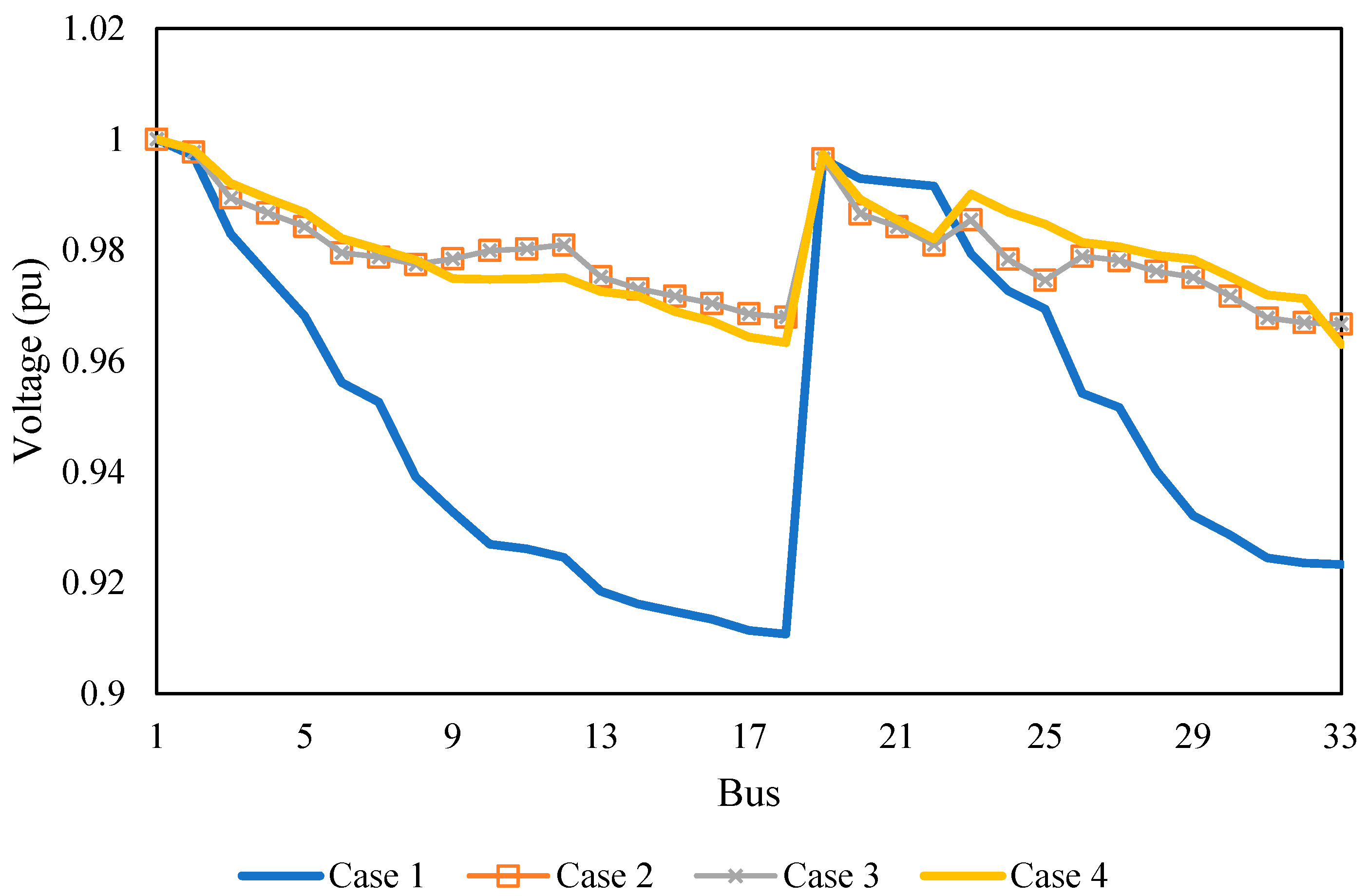
| 3 | 87.049 | 0.9667 | 12–22, 25–29 | 0.76/−0.76, −0.40/0.40 | 0.42/0.12, 0.41/1.03 | 33, 34, 35, 36, 37 | |
| 4 | 74.137 | 0.9630 | 25–29, 19–20 | 2.49/−1.89, −1.29/1.29 | 0.15/1.33, 0.58/0.24 | 19, 14, 9, 32, 37 | |
| TLBO | 2 | 141.431 | 0.9383 | 7, 14, 9, 36, 37 | |||
| 3 | 93.032 | 0.9622 | 30–31, 19–20 | −0.47/0.47, −1.31/1.31 | 0.66/0.43, 0.37/0.41 | 19, 34, 35, 30, 37 | |
| 4 | 87.092 | 0.9682 | 25–29, 12–13 | −0.40/0.40, −0.31/0.31 | 0.51/1.02, 0.18/0.28 | 7, 12, 10, 36, 37 | |
| CO | 2 | 142.135 | 0.9400 | 7, 34, 11, 32, 37 | |||
| 3 | 96.652 | 0.9606 | 25–29, 8–21 | −0.12/0.12, −1.16/1.16 | 0.73/0.79, 0.15/0.64 | 33, 34, 35, 36, 37 | |
| 4 | 99.761 | 0.9630 | 14–15, 28–29 | −0.24/0.24, −0.54/0.54 | 0.61/0.19, 0.00/0.87 | 7, 14, 10, 36, 28 | |
| PSO | 2 | 150.941 | 0.9316 | 33, 34, 9, 17, 28 | |||
| 3 | 90.310 | 0.9528 | 19–20, 25–29 | −1.23/1.23, −0.37/0.37 | 0.19/0.44, 0.42/1.09 | 19, 34, 35, 36, 37 | |
| 4 | 94.525 | 0.9620 | 12–22, 5–6 | 0.65/−0.65, −1.29/1.29 | 0.50/0.16, 0.32/0.99 | 5, 34, 35, 10, 37 | |
| JAYA | 2 | 144.811 | 0.9397 | 33, 34, 11, 32, 28 | |||
| 3 | 95.343 | 0.9490 | 25–29, 7–8 | −0.23/0.23, −1.29/1.29 | 0.46/1.03, 0.26/0.39 | 5, 34, 35, 36, 37 | |
| 4 | 87.821 | 0.9662 | 25–29, 3–4 | −0.42/0.42, −1.10/1.10 | 0.22/1.05, 0.60/0.43 | 3, 14, 9, 36, 37 |
| Algorithm | Case | Power Loss (kW) | Min Voltage (p.u.) | SOP Location (Node s/Node r) | SOP Active Power (MW) | SOP Reactive Power (MVAR) | Open Switches |
|---|---|---|---|---|---|---|---|
| 1 | 224.992 | 0.9092 | 69, 70, 71, 72, 73 | ||||
| hTLBO-CO | 2 | 99.619 | 0.9428 | 69, 70, 14, 57, 61 | |||
| 3 | 45.941 | 0.9793 | (15–46), (50–59) | 0.44/−0.44, −1.59/1.59 | 0.36/0.07, 0.55/1.28 | 69, 70, 71, 72, 73 | |
| 4 | 40.234 | 0.9814 | (50–59), (61–62) | −1.39/1.39, −0.16/0.16 | 0.54/0.43, 0.64/0.31 | 69, 70, 12, 72, 61 | |
| TLBO | 2 | 105.313 | 0.9428 | 10, 70, 14, 58, 61 | |||
| 3 | 45.980 | 0.9797 | (15–46), (50–59) | 0.44/−0.44, −1.61/1.61 | 0.36/0.09, 0.64/1.27 | 69, 70, 71, 72, 73 | |
| 4 | 77.705 | 0.9610 | (5–6), (27–65) | −0.94/0.94, −0.47/0.47 | 0.82/0.34, 0.24/0.86 | 5, 20, 71, 58, 73 | |
| CO | 2 | 99.619 | 0.9428 | 69, 70, 14, 57, 61 | |||
| 3 | 54.326 | 0.9796 | (27–65), (50–59) | 0.01/−0.01, −1.76/1.76 | 0.43/0.49, 0.56/0.74 | 69, 70, 71, 72, 73 | |
| 4 | 83.248 | 0.9614 | (7–8), (54–55) | −1.09/1.09, −0.50/0.50 | 0.72/0.75, 0.37/0.59 | 7, 18, 14, 54, 62 | |
| PSO | 2 | 99.619 | 0.9428 | 69, 70, 14, 57, 61 | |||
| 3 | 50.698 | 0.9791 | (50–59), (15–46) | −1.59/1.59, 0.44/−0.44 | 0.55/1.35, 0.00/0.07 | 69, 70, 71, 72, 73 | |
| 4 | 58.889 | 0.9805 | (50–59), (27–65) | −1.67/1.67, −0.02/0.02 | 0.55/0.00, 0.35/0.95 | 69, 16, 71, 72, 73 | |
| JAYA | 2 | 99.619 | 0.9428 | 69, 70, 14, 57, 61 | |||
| 3 | 55.794 | 0.9782 | (50–59), (27–65) | −1.77/1.77, 0.22/−0.22 | 0.44/1.07, 0.39/0.38 | 69, 70, 71, 72, 73 | |
| 4 | 61.391 | 0.9580 | (50–59), (11–43) | −1.38/1.38, 0.66/−0.66 | 0.03/1.06, 0.95/0.18 | 69, 70, 71, 72, 63 |
| Algorithm | Case | Power Loss (kW) | Min Voltage (p.u.) | SOP Location (Branch) | SOP Active Power (MW) | SOP Reactive Power (MVAR) | Open Switches |
|---|---|---|---|---|---|---|---|
| 1 | 1298.09 | 0.86880 | 118, 119, 120, 121, 122, 123, 124, 125, 126, 127, 128, 129, 130, 131, 132 | ||||
| hTLBO-CO | 2 | 645.0853797 | 0.932287185 | 42, 25, 20, 51, 47, 61, 39, 125, 89, 78, 90, 129, 130, 108, 32 | |||
| 3 | 618.9295667 | 0.954703163 | 120, 127, 122, 132, 131 | −2.32/2.32, −1.44/1.44, −0.04/0.04, −2.21/2.21, 1.69/−1.69 | 0.44/0.24, 1.09/1.74, 0.43/2.32, 0.37/0.56, 1.85/0.26 | 118, 119, 120, 121, 122, 123, 124, 125, 126, 127, 128, 129, 130, 131, 132 | |
| 4 | 601.0983882 | 0.957333363 | 122, 130, 126, 109, 132 | −0.11/0.11, −0.46/0.46, 0.40/−0.40, −0.19/0.19, −1.67/1.67 | 0.55/1.87, 0.81/2.39, 0.71/1.17, 0.73/1.50, 0.71/1.09 | 118, 119, 23, 121, 122, 123, 124, 125, 126, 73, 128, 129, 130, 109, 132 | |
| TLBO | 2 | 1023.286911 | 0.904298915 | 41, 119, 22, 48, 50, 59, 37, 57, 68, 73, 97, 82, 104, 109, 32 | |||
| 3 | 639.3315537 | 0.952421454 | 131, 129, 126, 122, 127 | 1.45/−1.45, −0.14/0.14, 0.41/−0.41, −0.48/0.48, −1.14/1.14 | 1.46/0.22, 1.08/0.79, 1.54/1.18, 0.59/2.45, 0.67/0.00 | 118, 119, 120, 121, 122, 123, 124, 125, 126, 127, 128, 129, 130, 131, 132 | |
| 4 | 629.9023748 | 0.943755842 | 127, 131, 132, 132, 120 | −1.07/1.07, 1.34/−1.34, −0.26/0.26, −1.71/1.71, −2.31/2.31 | 1.35/1.62, 2.11/0.00, 0.30/2.48, 0.05/0.00, 0.96/0.21 | 118, 119, 120, 121, 122, 123, 124, 125, 71, 127, 128, 129, 130, 131, 132 | |
| CO | 2 | 888.9398521 | 0.931624171 | 42, 26, 22, 51, 122, 58, 38, 90, 70, 87, 128, 129, 130, 109, 33 | |||
| 3 | 631.6124428 | 0.943894417 | 131, 132, 124, 126, 127 | 1.33/−1.33, −0.32/0.32, −1.59/1.59, 0.45/−0.45, −1.10/1.10 | 2.11/0.24, 0.58/2.48, 1.67/1.35, 1.04/1.21, 1.16/0.49 | 118, 119, 120, 121, 122, 123, 124, 125, 126, 127, 128, 129, 130, 131, 132 | |
| 4 | 623.1575736 | 0.94499893 | 125, 131, 130, 132, 122 | −0.70/0.70, 1.69/−1.69, −0.52/0.52, −1.73/1.73, 0.05/−0.05 | 0.38/1.99, 1.84/0.99, 1.54/2.01, 1.81/2.05, 0.91/0.83 | 118, 119, 20, 121, 122, 58, 124, 125, 72, 73, 75, 129, 130, 131, 132 | |
| PSO | 2 | 973.4293657 | 0.894487966 | 45, 119, 120, 121, 32, 123, 5, 90, 66, 87, 128, 129, 130, 109, 9 | |||
| 3 | 630.9999426 | 0.953725123 | 120, 131, 123, 127, 122 | −0.54/0.54, 1.28/−1.28, −1.63/1.63, −1.38/1.38, −1.59/1.59 | 0.00/0.59, 2.15/0.05, 0.00/0.56, 1.33/1.59, 0.00/2.02 | 118, 119, 120, 121, 122, 123, 124, 125, 126, 127, 128, 129, 130, 131, 132 | |
| 4 | 893.865821 | 0.89934752 | 132, 132, 132, 131, 132 | −1.93/1.93, −2.50/2.50, 1.78/−1.78, 1.42/−1.42, 2.50/−2.50 | 0.00/1.59, 0.01/1.51, 0.78/0.00, 2.06/0.00, 0.00/0.00 | 118, 12, 120, 121, 122, 123, 124, 125, 126, 127, 73, 82, 85, 131, 132 | |
| JAYA | 2 | 910.9940056 | 0.932115899 | 42, 15, 23, 50, 47, 57, 124, 90, 71, 127, 76, 81, 130, 108, 132 | |||
| 3 | 705.7003877 | 0.942542197 | 124, 126, 132, 127, 131 | −2.50/2.50, 0.69/−0.69, −0.36/0.36, −0.64/0.64, 1.93/−1.93 | 0.05/0.36, 1.88/0.40, 0.67/2.41, 0.99/0.12, 1.59/0.93 | 118, 119, 120, 121, 122, 123, 124, 125, 126, 127, 128, 129, 130, 131, 132 | |
| 4 | 857.935727 | 0.913523291 | 131, 132, 132, 125, 132 | 1.00/−1.00, 0.93/−0.93, −2.48/2.48, 0.19/−0.19, 1.92/−1.92 | 2.00/0.58, 0.00/1.64, 0.34/0.06, 0.00/0.67, 1.60/1.43 | 118, 12, 22, 121, 122, 123, 124, 125, 71, 127, 128, 129, 85, 131, 132 |
| Algorithm | Final Solution (kW) | Total Improvement (%) | Iterations to 95% | Iterations to 99% | Phase 1 Rate (kW/iter) | Relative Performance * |
|---|---|---|---|---|---|---|
| Case 2 | ||||||
| hTLBO-CO | 138.928 | 17.69 | 14 | 27 | 0.4975 | Benchmark |
| TLBO | 141.431 | 11.21 | 6 | 12 | 0.2977 | +1.80% |
| CO | 142.135 | 15.79 | 94 | 123 | 0.3117 | +2.31% |
| PSO | 150.942 | 11.36 | 5 | 5 | 0.3224 | +8.65% |
| JAYA | 144.811 | 10.59 | 8 | 28 | 0.2858 | +4.24% |
| Case 3 | ||||||
| hTLBO-CO | 87.049 | 17.64 | 14 | 21 | 0.3101 | Benchmark |
| TLBO | 93.032 | 39.64 | 35 | 132 | 0.9873 | +6.87% |
| CO | 96.652 | 33.47 | 85 | 291 | 0.4671 | +11.03% |
| PSO | 90.310 | 29.35 | 11 | 23 | 0.6254 | +3.75% |
| JAYA | 95.343 | 13.98 | 66 | 76 | 0.1510 | +9.53% |
| Case 4 | ||||||
| hTLBO-CO | 74.137 | 52.06 | 74 | 151 | 1.2564 | Benchmark |
| TLBO | 87.092 | 44.00 | 37 | 118 | 1.0725 | +17.47% |
| CO | 99.761 | 70.84 | 172 | 289 | 2.2512 | +34.56% |
| PSO | 94.525 | 30.45 | 19 | 28 | 0.6898 | +27.50% |
| JAYA | 87.821 | 37.85 | 71 | 186 | 0.7392 | +18.46% |
| Algorithm | Final Solution (kW) | Total Improvement (%) | Iterations to 95% | Iterations to 99% | Phase 1 Rate (kW/iter) | Convergence Efficiency |
|---|---|---|---|---|---|---|
| Case 2 | ||||||
| hTLBO-CO | 99.629 | 18.46 | 10 | 23 | 0.3759 | Balanced |
| TLBO | 105.323 | 11.59 | 29 | 42 | 0.2301 | Inefficient |
| CO | 99.629 | 40.78 | 171 | 171 | 0.5863 | Very Slow |
| PSO | 99.629 | 15.95 | 2 | 5 | 0.3151 | Very Fast |
| JAYA | 99.629 | 21.33 | 5 | 6 | 0.4503 | Fast |
| Case 3 | ||||||
| hTLBO-CO | 45.941 | 44.81 | 65 | 95 | 0.5682 | Best Solution |
| TLBO | 45.980 | 47.58 | 40 | 69 | 0.6833 | Very Close |
| CO | 54.326 | 40.34 | 255 | 279 | 0.4432 | Poor |
| PSO | 50.698 | 19.07 | 9 | 14 | 0.1991 | Fast but Suboptimal |
| JAYA | 55.794 | 12.95 | 24 | 43 | 0.1353 | Inefficient |
| Case 4 | ||||||
| hTLBO-CO | 40.234 | 25.07 | 165 | 261 | 0.0990 | Benchmark |
| TLBO | 77.705 | 65.73 | 64 | 124 | 2.4189 | +93.13% |
| CO | 83.248 | 76.42 | 22 | 255 | 4.4327 | +106.91% |
| PSO | 58.889 | 45.95 | 22 | 28 | 0.8344 | +46.37% |
| JAYA | 61.391 | 53.38 | 250 | 279 | 0.7452 | +52.58% |
| Algorithm | Final Solution (kW) | Total Improvement (%) | Iterations to 95% | Iterations to 99% | Performance Gap vs. Best | |
|---|---|---|---|---|---|---|
| Case 2 | ||||||
| hTLBO-CO | 645.085 | 50.30 | 208 | 277 | Benchmark | |
| TLBO | 1023.287 | 55.85 | 106 | 125 | +58.63% | |
| CO | 888.940 | 99.99 | 74 | 191 | +37.80% | |
| PSO | 973.429 | 99.79 | 9 | 9 | +50.90% | |
| JAYA | 910.994 | 100.00 | 586 | 596 | +41.22% | |
| Case 3 | ||||||
| hTLBO-CO | 618.930 | 28.87 | 377 | 842 | 0.9723 | Benchmark |
| TLBO | 674.709 | 18.58 | 36 | 83 | 0.7695 | +9.01% |
| CO | 631.612 | 47.32 | 102 | 132 | 2.8321 | +2.05% |
| PSO | 631.000 | 30.56 | 22 | 28 | 1.3885 | +1.95% |
| JAYA | 705.700 | 25.84 | 97 | 97 | 1.2293 | +14.02% |
| Case 4 | ||||||
| hTLBO-CO | 601.098 | 99.08 | 125 | 181 | 324.662 | Benchmark |
| TLBO | 629.902 | 94.36 | 364 | 536 | 52.411 | +4.79% |
| CO | 623.158 | 80.49 | 422 | 815 | 11.881 | +3.67% |
| PSO | 893.866 | 82.15 | 22 | 27 | 20.564 | +48.71% |
| JAYA | 857.936 | 76.81 | 672 | 909 | 13.082 | +42.73% |
| Algorithm | Best (kW) | Mean ± Std (kW) | Max (kW) | Mean Rank | Computation Time (s) | Statistical Significance vs. hTLBO-CO |
|---|---|---|---|---|---|---|
| Case 2 | ||||||
| hTLBO-CO | 138.928 | 140.912 ± 1.351 | 142.950 | 1.0 | 81.9 | Benchmark |
| TLBO | 141.431 | 146.725 ± 5.462 | 157.230 | 2.4 | 101.4 | p = 0.001953 * |
| CO | 142.135 | 146.151 ± 2.698 | 150.180 | 2.7 | 67.9 | p = 0.001953 * |
| PSO | 150.941 | 156.851 ± 5.644 | 170.780 | 4.9 | 49.2 | p = 0.001953 * |
| JAYA | 144.811 | 150.202 ± 5.464 | 161.650 | 4.0 | 70.8 | p = 0.001953 * |
| Case 3 | ||||||
| hTLBO-CO | 87.049 | 88.714 ± 1.180 | 90.470 | 1.0 | 97.8 | Benchmark |
| PSO | 90.310 | 96.928 ± 7.977 | 114.510 | 2.6 | 91.0 | p = 0.001953 * |
| TLBO | 93.032 | 96.677 ± 3.316 | 103.460 | 3.1 | 169.5 | p = 0.001953 * |
| JAYA | 95.343 | 99.340 ± 3.880 | 108.220 | 3.7 | 96.0 | p = 0.001953 * |
| CO | 96.652 | 100.774 ± 3.686 | 108.650 | 4.6 | 94.8 | p = 0.001953 * |
| Case 4 | ||||||
| hTLBO-CO | 74.137 | 76.080 ± 1.326 | 78.120 | 1.0 | 85.7 | Benchmark |
| TLBO | 87.092 | 89.857 ± 1.874 | 92.860 | 2.3 | 112.3 | p = 0.001953 * |
| JAYA | 87.821 | 91.213 ± 2.176 | 94.660 | 3.1 | 98.4 | p = 0.001953 * |
| PSO | 94.525 | 98.642 ± 2.654 | 102.790 | 3.8 | 75.9 | p = 0.001953 * |
| CO | 99.761 | 103.754 ± 2.654 | 107.780 | 4.8 | 83.2 | p = 0.001953 * |
| Algorithm | Best (kW) | Mean ± Std (kW) | Max (kW) | Mean Rank | Computation Time (s) | Statistical Significance vs. hTLBO-CO |
|---|---|---|---|---|---|---|
| Case 2 | ||||||
| hTLBO-CO | 99.62 | 102.56 ± 2.83 | 109.42 | 1.35 | 87.00 | Benchmark |
| CO | 99.62 | 105.30 ± 4.48 | 112.85 | 2.65 | 66.30 | p = 0.044 * |
| JAYA | 99.62 | 109.52 ± 9.91 | 125.20 | 2.85 | 91.08 | p = 0.058 |
| PSO | 99.62 | 109.66 ± 7.04 | 121.05 | 3.95 | 78.90 | p = 0.009 * |
| TLBO | 105.31 | 110.35 ± 4.21 | 118.63 | 4.20 | 95.40 | p = 0.001953 * |
| Case 3 | ||||||
| hTLBO-CO | 45.94 | 48.32 ± 2.15 | 53.29 | 1.1 | 128.40 | Benchmark |
| TLBO | 45.98 | 51.91 ± 7.05 | 66.03 | 2.3 | 219.10 | p = 0.049 * |
| PSO | 50.70 | 60.84 ± 14.82 | 89.14 | 3.3 | 122.07 | p = 0.001953 * |
| CO | 54.33 | 59.33 ± 6.29 | 76.30 | 3.8 | 121.40 | p = 0.001953 * |
| JAYA | 55.79 | 66.06 ± 15.38 | 98.40 | 4.5 | 121.50 | p = 0.001953 * |
| Case 4 | ||||||
| hTLBO-CO | 40.23 | 45.59 ± 6.30 | 60.11 | 1.0 | 79.80 | Benchmark |
| PSO | 58.89 | 75.72 ± 20.60 | 113.40 | 2.6 | 126.60 | p = 0.001953 * |
| JAYA | 61.39 | 80.24 ± 23.22 | 124.22 | 3.1 | 99.30 | p = 0.001953 * |
| TLBO | 77.71 | 89.37 ± 10.58 | 108.11 | 3.7 | 138.57 | p = 0.001953 * |
| CO | 83.25 | 101.53 ± 8.48 | 111.01 | 4.6 | 83.70 | p = 0.001953 * |
| Algorithm | Best (kW) | Mean ± Std (kW) | Max (kW) | Mean Rank | Computation Time (s) | Statistical Significance vs. hTLBO-CO |
|---|---|---|---|---|---|---|
| Case 2 | ||||||
| hTLBO-CO | 645.085 | 670.213 ± 18.010 | 702.536 | 1.0 | 514.00 | Benchmark |
| CO | 888.940 | 937.586 ± 32.812 | 986.232 | 2.0 | 328.40 | p = 0.001953 * |
| JAYA | 910.994 | 965.929 ± 37.298 | 1017.087 | 3.0 | 316.02 | p = 0.001953 * |
| PSO | 973.429 | 1034.220 ± 48.786 | 1123.560 | 4.1 | 702.60 | p = 0.001953 * |
| TLBO | 1023.287 | 1079.254 ± 37.736 | 1135.220 | 4.9 | 508.80 | p = 0.001953 * |
| Case 3 | ||||||
| hTLBO-CO | 618.93 | 640.036 ± 14.254 | 661.141 | 1.0 | 1301.6 | Benchmark |
| CO | 631.61 | 657.464 ± 20.904 | 701.200 | 2.5 | 1163.8 | p = 0.001953 * |
| PSO | 631.00 | 669.846 ± 36.204 | 752.350 | 2.9 | 1228.8 | p = 0.001953 * |
| TLBO | 639.33 | 665.134 ± 19.552 | 700.650 | 3.7 | 2068.1 | p = 0.001953 * |
| JAYA | 705.70 | 739.425 ± 34.177 | 824.520 | 4.9 | 1185.7 | p = 0.001953 * |
| Case 4 | ||||||
| hTLBO-CO | 601.098 | 626.410 ± 20.099 | 663.360 | 1.2 | 512.35 | Benchmark |
| CO | 623.158 | 649.175 ± 26.666 | 715.700 | 2.0 | 528.03 | p = 0.003906 * |
| TLBO | 629.902 | 662.684 ± 38.370 | 763.540 | 2.8 | 694.30 | p = 0.003906 * |
| JAYA | 857.936 | 908.110 ± 72.973 | 1108.780 | 4.1 | 385.50 | p = 0.001953 * |
| PSO | 893.866 | 947.815 ± 60.689 | 1105.400 | 4.9 | 808.84 | p = 0.001953 * |
| Number of SOPs | Minimum Voltage (pu) | Power Loss (kW) | Performance Classification |
|---|---|---|---|
| 15 | 0.9597 | 535.37 | High-Investment Region |
| 14 | 0.9539 | 571.41 | High-Investment Region |
| 13 | 0.9495 | 622.22 | High-Investment Region |
| 12 | 0.9478 | 607.18 | High-Investment Region |
| 11 | 0.9463 | 614.58 | Optimal Compromise Region |
| 10 | 0.9418 | 621.94 | Optimal Compromise Region |
| 9 | 0.9442 | 619.50 | Optimal Compromise Region |
| 8 | 0.9489 | 617.28 | Optimal Compromise Region |
| 7 | 0.9570 | 622.06 | Optimal Compromise Region |
| 6 | 0.9552 | 609.85 | Optimal Compromise Region |
| 5 | 0.9573 | 601.10 | Cost-Effective Region |
| 4 | 0.9501 | 675.16 | Cost-Effective Region |
| 3 | 0.9389 | 712.89 | Cost-Effective Region |
| 2 | 0.9246 | 743.59 | Cost-Effective Region |
| 1 | 0.8993 | 816.01 | Cost-Effective Region |
| Method | Opened Switches | Power LOSS (kW) | Loss Reduction (%) | Min Voltage (p.u.) |
|---|---|---|---|---|
| Initial | 118–119–120–121–122–123–124–125–126–127–128–129–130–131–132 | 1298.09 | – | 0.8688 |
| ITS [34] | 42–26–23–51–122–58–39–95–74–71–97–129–130–109–34 | 867.40 | 33.18 | 0.9323 |
| MTS [35] | 42–26–23–51–122–58–39–95–74–71–97–129–130–109–34 | 867.40 | 33.18 | 0.9323 |
| FWA [36] | 42–25–23–121–50–58–39–95–71–74–97–129–130–109–34 | 854.06 | 34.20 | 0.9298 |
| CSA [37] | 42–25–23–121–50–58–39–95–71–74–97–129–130–109–34 | 855.04 | 34.13 | 0.9298 |
| HSA [38] | 23–27–33–43–53–62–72–75–123–125–126–129–130–131–132 | 854.21 | 34.19 | 0.9323 |
| FA [39] | 24–26–35–40–43–51–59–72–75–96–98–110–122–130–131 | 854.06 | 34.20 | 0.9323 |
| SFS [40] | 23–25–34–39–42–50–58–71–74–95–97–109–121–129–130 | 854.04 | 34.20 | 0.9323 |
| SSOE [41] | 23–25–34–39–42–50–58–71–74–95–97–109–121–129–130 | 853.60 | 34.16 | 0.9323 |
| MSSOE [42] | 23–26–34–39–42–50–58–71–74–95–97–109–121–129–130 | 854.03 | 34.13 | 0.9323 |
| CGA-ISP [43] | 23–25–34–39–42–50–58–71–74–95–97–109–121–129–130 | 855.04 | 34.00 | 0.9290 |
| ARO [44] | 23–43–120–51–122–61–39–95–71–74–97–129–130–109–132 | 851.01 | 34.36 | 0.9412 |
| Proposed hTLBO-CO | 42–25–20–51–47–61–39–125–89–78–90–129–130–108–32 | 645.09 | 50.30 | 0.9323 |
Disclaimer/Publisher’s Note: The statements, opinions and data contained in all publications are solely those of the individual author(s) and contributor(s) and not of MDPI and/or the editor(s). MDPI and/or the editor(s) disclaim responsibility for any injury to people or property resulting from any ideas, methods, instructions or products referred to in the content. |
© 2025 by the authors. Licensee MDPI, Basel, Switzerland. This article is an open access article distributed under the terms and conditions of the Creative Commons Attribution (CC BY) license (https://creativecommons.org/licenses/by/4.0/).
Share and Cite
Alanazi, A.; Alanazi, M.; Alruwaili, M. A Hybrid TLBO-Cheetah Algorithm for Multi-Objective Optimization of SOP-Integrated Distribution Networks. Mathematics 2025, 13, 3419. https://doi.org/10.3390/math13213419
Alanazi A, Alanazi M, Alruwaili M. A Hybrid TLBO-Cheetah Algorithm for Multi-Objective Optimization of SOP-Integrated Distribution Networks. Mathematics. 2025; 13(21):3419. https://doi.org/10.3390/math13213419
Chicago/Turabian StyleAlanazi, Abdulaziz, Mohana Alanazi, and Mohammed Alruwaili. 2025. "A Hybrid TLBO-Cheetah Algorithm for Multi-Objective Optimization of SOP-Integrated Distribution Networks" Mathematics 13, no. 21: 3419. https://doi.org/10.3390/math13213419
APA StyleAlanazi, A., Alanazi, M., & Alruwaili, M. (2025). A Hybrid TLBO-Cheetah Algorithm for Multi-Objective Optimization of SOP-Integrated Distribution Networks. Mathematics, 13(21), 3419. https://doi.org/10.3390/math13213419


