Asymptotic Analysis of the Bias–Variance Trade-Off in Subsampling Metropolis–Hastings

Abstract

Markov chain Monte Carlo (MCMC) methods are fundamental to Bayesian inference but are often computationally prohibitive for large datasets, as the full likelihood must be evaluated at each iteration. Subsampling-based approximate Metropolis–Hastings (MH) algorithms offer a popular alternative, trading a manageable bias for a significant reduction in per-iteration cost. While this bias–variance trade-off is empirically understood, a formal theoretical framework for its optimization has been lacking. Our work establishes such a framework by bounding the mean squared error (MSE) as a function of the subsample size (m), the data size (n), and the number of epochs (E). This analysis reveals two optimal asymptotic scaling laws: the optimal subsample size is $m^{★}=O\left(E^{1/2}\right)$, leading to a minimal MSE that scales as ${\mathrm{MSE}}^{★}=O\left(E^{-1/2}\right)$. Furthermore, leveraging the large-sample asymptotic properties of the posterior, we show that when augmented with a control variate, the approximate MH algorithm can be asymptotically more efficient than the standard MH method under ideal conditions. Experimentally, we first validate the two optimal asymptotic scaling laws. We then use Bayesian logistic regression and Softmax classification models to highlight a key difference in convergence behavior: the exact algorithm starts with a high MSE that gradually decreases as the number of epochs increases. In contrast, the approximate algorithm with a practical control variate maintains a consistently low MSE that is largely insensitive to the number of epochs.

1. Introduction

The scalability of standard Markov chain Monte Carlo (MCMC) methods for posterior inference is a critical challenge in the era of large datasets. The primary bottleneck is the computational cost of evaluating the full likelihood, $\pi \left(\theta \right)\propto p\left(\theta \right){\prod }_{i=1}^{n}p\left(x_i\right|\theta )$, at each iteration, a task that becomes prohibitive as the data size n grows. This computational bottleneck is the central challenge in modern Bayesian inference. To address this, a significant research effort has shifted towards developing scalable MCMC algorithms, a field comprehensively reviewed in [1,2]. These approaches generally follow two main paradigms. The former adapts the MCMC framework for parallel execution, decomposing the computational problem into tasks that can be processed concurrently [3,4,5,6,7,8,9]. The latter focuses on fundamentally modifying the algorithm itself, rendering it scalable by avoiding a full evaluation of the likelihood [10,11,12,13,14,15]. Delving deeper into the latter approach, a significant thrust involves the development of approximate MCMC. Many of these methods build upon the foundational MH framework, adapting it for large-scale problems [16,17,18]. The central idea is to replace the exact, but costly, likelihood calculation over the entire dataset with a more tractable approximation. Two prominent strategies have emerged in this area. One involves constructing a surrogate model to approximate the likelihood function [18,19,20], a method whose primary limitation lies in the challenge of building a sufficiently accurate surrogate and quantifying its approximation error. Another approach, into which the research of this paper falls, directly computes the likelihood on a smaller subset of the data. The use of such a subset, however, often relies on a biased or noisy likelihood estimator. As established in [21], this introduces a discrepancy between the stationary distribution of the resulting Markov chain and the true target distribution. This inherent approximation gap is precisely why this class of methods is termed “approximate MH” or “noisy MH” algorithms [22].

The performance of such subsampling methods critically depends on the composition and size of the chosen subset. Regarding composition, some strategies are motivated by the principle that not all data points contribute equally to the final estimator [16,23]. These methods, therefore, aim to construct more informative subsets by selecting points based on their respective contributions, rather than purely at random. In contrast, another prominent approach, explored in works such as [24,25], uses a uniformly random subset of data to form an unbiased log-likelihood estimate. A key feature of these latter frameworks is that the subset size is dynamically adjusted in each iteration, governed by the criterion that the resulting bias must be kept below a pre-specified constant. However, this tuning criterion does not account for computational complexity. Subsequent work [17] addressed this by using a criterion based on minimizing the time required to generate one effectively independent posterior sample. While theoretically appealing, this approach has its own limitations due to its reliance on the pseudo-marginal MCMC framework [21,26,27]. A significant drawback of the pseudo-marginal method is the risk of the Markov chain becoming trapped in regions where the likelihood is overestimated. Moreover, its requirement for a positive, unbiased likelihood estimator is notoriously difficult to satisfy in practice, as highlighted by [28], with some approaches only yielding nearly unbiased estimators [17].

In this study, we conduct a rigorous analysis of the approximate MH algorithm. As our primary evaluation criterion, we use a cost-aware MSE of the posterior estimator. Building upon the general framework of Johndrow et al. [29], we specialize the analysis to well-behaved MCMC kernels with small approximation errors. We establish a theoretical framework that bounds the MSE as a function of the subsample size m, the total data size n, and the number of epochs E. This analysis of the bias–variance trade-off reveals the optimal asymptotic scaling laws: the ideal subsample size is $m^{★}=O\left(E^{1/2}\right)$, resulting in a minimal MSE that scales as ${\mathrm{MSE}}^{★}=O\left(E^{-1/2}\right)$. Furthermore, our analysis reveals that the variance of the subsampling-based estimator is a primary driver of the final posterior MSE. This insight motivates the application of variance-reduction techniques, such as control variates, whose theoretical underpinnings are entirely different from those of the pseudo-marginal MCMC framework [17]. Under the large-sample asymptotic regime of the posterior [30], we find that applying the control variate method under ideal conditions can render the approximate algorithm asymptotically more efficient than the exact algorithm, even permitting the optimal subsample size to be chosen independently of the total data size n. We demonstrate this convergence advantage on Generalized Linear Models, which are the subject of extensive research for various statistical challenges [31].

The remainder of this paper is structured as follows. Section 2 develops a theoretical framework for the MSE of the approximate Metropolis–Hastings estimator. Our analysis of the asymptotic bias–variance trade-off establishes the optimal scaling laws for the algorithm. We show that the ideal subsample size scales as $m^{★}=O\left(E^{1/2}\right)$, which in turn yields a minimal MSE with a convergence rate of $O\left(E^{-1/2}\right)$. We conclude the section with a simple toy example that provides an empirical validation of these theoretical scaling relationships. In Section 3, we extend this analysis to the asymptotic regime of the posterior distribution. We find that a key quantity affecting the MSE, the uniform expected standard deviation of the log-likelihood ratio, decreases as a function of the total data size, n. We further demonstrate that, under ideal conditions, incorporating a control variate allows the approximate algorithm to become asymptotically more efficient than the exact algorithm. Finally, Section 4 presents extensive experiments that empirically validate our theoretical findings.

2. Asymptotic Optimization of the Approximate MH

This section develops a rigorous theoretical framework for analyzing the MSE of the approximate MH algorithm’s posterior estimates. We establish a formal bound on the MSE as a function of several key factors, including the subsample size, the total data size, and the computational budget. This framework is crucial as it enables the subsequent asymptotic optimization of the algorithm. Prior to this analysis, we briefly review the fundamental concepts of the relevant MH algorithms.

2.1. Approximate MH Algorithm

The MH algorithm is a foundational MCMC method, valued for its simplicity and ease of implementation. It is designed to generate samples from a target posterior distribution $\pi \left(\theta \right)\propto p\left(\theta \right){\prod }_{i=1}^{n}p(x_i\mid \theta )$, where $p\left(\theta \right)$ is the prior and $p(x_i\mid \theta )$ is the likelihood for each data point.

The algorithm proceeds by initializing a Markov chain at a starting point ${\theta }^{\left(0\right)}$. At each subsequent iteration, a candidate state ${\theta }^{\prime }$ is drawn from a proposal distribution $q({\theta }^{\prime }\mid \theta )$ that depends on the current state $\theta$. This candidate is then accepted with a probability given by

$$\alpha (\theta ,{\theta }^{\prime })=min\left(1,{\displaystyle \frac{\pi \left({\theta }^{\prime }\right)q(\theta \mid {\theta }^{\prime })}{\pi \left(\theta \right)q({\theta }^{\prime }\mid \theta )}}\right).$$

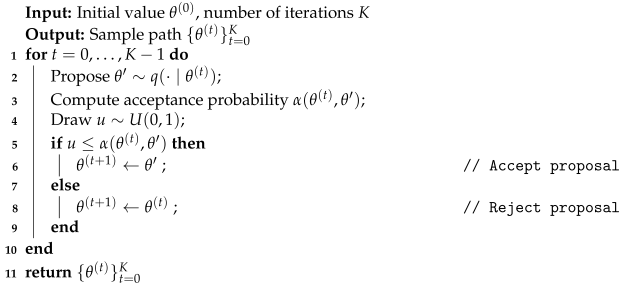
If the candidate is accepted, the chain moves to the new state; otherwise, it remains at the current state. This process generates a Markov chain whose stationary distribution is the desired posterior $\pi \left(\theta \right)$. The specific procedure is outlined in Algorithm 1. To distinguish it from the approximate variants discussed later, we will refer to this as the exact algorithm.

Algorithm 1: The Metropolis–Hastings Algorithm

The primary computational bottleneck in the MH algorithm is the evaluation of the full likelihood, which is required to compute the acceptance probability at each iteration. To analyze its dependence on the sample size n, we first express the acceptance probability in terms of the log-likelihood ratio, $\ell (\theta ,{\theta }^{\prime })$. This ratio is the sum of contributions from each data point:

$$\ell (\theta ,{\theta }^{\prime })=\sum _{i=1}^n{\ell }_i(\theta ,{\theta }^{\prime })=\sum _{i=1}^n\left(logp(x_i\mid {\theta }^{\prime })-logp(x_i\mid \theta )\right).$$

(1)

The acceptance probability can then be written compactly as $\alpha (\theta ,{\theta }^{\prime })=1\wedge e^{\mathcal{L}(\theta ,{\theta }^{\prime })}$, where $\mathcal{L}(\theta ,{\theta }^{\prime })$ contains the log-prior and log-proposal ratios in addition to $\ell (\theta ,{\theta }^{\prime })$.

Approximate MH algorithms mitigate this bottleneck by replacing the exact log-likelihood ratio with an estimate. Specifically, at each iteration, a small subset of data $U_m=\{x_{u_1},\dots ,x_{u_m}\}$ is drawn uniformly at random with replacement. This reduces the per-iteration computational complexity from $\mathrm{\Theta }\left(n\right)$ to $\mathrm{\Theta }\left(m\right)$. The full log-likelihood ratio $\ell (\theta ,{\theta }^{\prime })$ is then replaced by its unbiased estimator:

$${\widehat{\ell }}_{U_m}(\theta ,{\theta }^{\prime })={\displaystyle \frac{n}{m}}\sum _{i=1}^m\left(logp(x_{u_i}\mid {\theta }^{\prime })-logp(x_{u_i}\mid \theta )\right).$$

This yields the approximate acceptance probability:

$$\widehat{\alpha }(\theta ,{\theta }^{\prime };U_m)=1\wedge e^{\widehat{\mathcal{L}}(\theta ,{\theta }^{\prime })},$$

(2)

where $\widehat{\mathcal{L}}(\theta ,{\theta }^{\prime })$ is identical to $\mathcal{L}(\theta ,{\theta }^{\prime })$ but uses the estimator ${\widehat{\ell }}_{U_m}(\theta ,{\theta }^{\prime })$.

The motivation for employing approximate MH algorithms stems from the need to efficiently estimate posterior quantities, such as the expectation ${\mathbb{E}}_{\pi }\left[f\left(\theta \right)\right]$. For a given computational budget, approximate MCMC methods can generate samples more rapidly, often leading to estimators with lower variance compared to exact algorithms that must process the entire dataset. This computational advantage, however, comes at the cost of introducing bias into the posterior estimates.

In the next subsection, we provide a rigorous theoretical analysis of this trade-off. We use the MSE of the estimator for ${\mathbb{E}}_{\pi }\left[f\left(\theta \right)\right]$ as our primary performance metric to conduct an asymptotic analysis of the bias–variance trade-off. Through this analysis, we aim to determine the optimal scaling of the subsample size that minimizes the MSE. Before proceeding with the detailed derivation, we first define the standard notation used in our theoretical discussion.

The total variation distance between two probability distributions with densities $\pi (·)$ and $\widehat{\pi }(·)$ is defined as

$$\parallel \pi -\widehat{\pi }{\parallel }_{TV}={\displaystyle \frac{1}{2}}\int |\pi \left(\theta \right)-\widehat{\pi }\left(\theta \right)|d\theta .$$

(3)

Furthermore, let $f\left(\theta \right)$ be a bounded function. The expectation of $f\left(\theta \right)$ with respect to a measure $\nu$ is given by

$${\mu }_f=\int f\left(\theta \right)\nu \left(d\theta \right).$$

(4)

For the MSE of a multivariate random variable $\theta \in {\mathbb{R}}^d$, we use the following definition:

$$\mathrm{MSE}\left(\theta \right)={\mathbb{E}[\parallel \theta -\mu \parallel }^2]=\mathbb{E}\left[\sum _{j=1}^d{({\theta }_j-{\mu }_j)}^2\right],$$

(5)

where $\parallel ·\parallel$ denotes the Euclidean norm and $\mu =\mathbb{E}\left[\theta \right]$.

2.2. Bias–Variance Trade-Off Analysis

This subsection provides a formal analysis of the MSE for the posterior estimates generated by the approximate MH algorithm. We establish a bound on this error as a function of the subsample size m, the total data size n, and the number of epochs E.

To ensure a fair comparison of computational costs, we adopt a definition of an epoch E similar to that in established work such as [1,32]. Specifically, one epoch represents the computational work required to evaluate the full log-likelihood across the whole dataset. Consequently, a computational budget of E epochs is equivalent to performing a total of $n\times E$ log-likelihood evaluations.

For a random walk proposal, the approximate MH algorithm differs from its exact counterpart solely in the acceptance rate. Consequently, any perturbation in the chain’s trajectory arises from the error in estimating this rate. Our analysis therefore commences by quantifying the deviation between the approximate and true acceptance rates. Unless otherwise noted, proofs for all results that follow are deferred to the Appendix A.

To derive the error bound for the estimated acceptance probability presented in Lemma 1, we first introduce two key assumptions regarding the properties of the log-likelihood ratios.

Assumption 1.

Suppose that for all $i\in \{1,\dots ,n\}$ and any $(\theta ,{\theta }^{\prime })\in {\mathrm{\Theta }}^2$, the deviation of each individual log-likelihood ratio from the mean is bounded by $\left|{\ell }_i(\theta ,{\theta }^{\prime })-\overline{\ell }(\theta ,{\theta }^{\prime })\right|\le R(\theta ,{\theta }^{\prime })$.

Assumption 2.

The log-likelihood function, $\ell \left(\theta \right)$, is L-Lipschitz continuous over the parameter space Θ. That is, there exists a constant $L>0$ such that for all ${\theta }_1,{\theta }_2\in \mathrm{\Theta }$,

$$|\ell \left({\theta }_1\right)-\ell \left({\theta }_2\right)|\le L\parallel {\theta }_1-{\theta }_2\parallel .$$

Lemma 1.

Let ${\ell }_i(\theta ,{\theta }^{\prime })=logp\left(x_i\right|{\theta }^{\prime })-logp\left(x_i\right|\theta )$ denote the individual log-likelihood ratio, calculated based on each of the n independent data samples. Let $U_m$ be a subsample of size m drawn uniformly at random with replacement. Define $\overline{\ell }(\theta ,{\theta }^{\prime })={\displaystyle \frac{1}{n}}{\sum }_{i=1}^n{\ell }_i(\theta ,{\theta }^{\prime })$ as the average log-likelihood ratio. Under Assumption 1, the mean absolute error of the estimated acceptance probability satisfies

$${\mathbb{E}}_{U_m}\left(\left|\widehat{\alpha }(\theta ,{\theta }^{\prime };U_m)-\alpha (\theta ,{\theta }^{\prime })\right|\right)\le ϵ\left(m,n,\sigma (\theta ,{\theta }^{\prime }),R(\theta ,{\theta }^{\prime })\right),$$

(6)

where the error bound $ϵ(·)$ is given by

$$ϵ(·)=2n\sigma (\theta ,{\theta }^{\prime })\sqrt{{\displaystyle \frac{ln(2/{\delta }_1)}{m}}}+{\displaystyle \frac{4nR(\theta ,{\theta }^{\prime })ln(2/{\delta }_1)}{3m}}+{\delta }_1.$$

(7)

Here, $\sigma (\theta ,{\theta }^{\prime })$ denotes the standard deviation of the log-likelihood ratios, defined as ${\sigma }^2(\theta ,{\theta }^{\prime })={\displaystyle \frac{1}{n}}{\sum }_{i=1}^n{({\ell }_i(\theta ,{\theta }^{\prime })-\overline{\ell }(\theta ,{\theta }^{\prime }))}^2$, and ${\delta }_1\in (0,1)$ is an arbitrarily small constant.

The preceding lemma establishes an upper bound on the mean absolute error of the acceptance probability. This bound, explicitly characterized by the error function $ϵ(·)$ in Equation (7), is pointwise, as it depends on the specific states $(\theta ,{\theta }^{\prime })$ under consideration. Building upon this result, Lemma 2 then derives a uniform error bound on the total variation distance between the approximate and exact transition kernels.

Lemma 2.

Under Assumption 2, the total variation distance between the approximate Metropolis–Hastings transition kernel, $\widehat{P}(\theta ,·)$, and the exact one, $P(\theta ,·)$, is bounded for any $\theta \in \mathrm{\Theta }$ as

$${∥\widehat{P}(\theta ,·)-P(\theta ,·)∥}_{\mathrm{TV}}\le {ϵ}^{★}.$$

The bound ${ϵ}^{★}=ϵ(m,n,{\sigma }_0,R_0)$ is obtained from the error function defined in Lemma 1 by using the constant upper bounds ${\sigma }_0$ and $R_0$, which are given by

$${\sigma }_0=\underset{\theta \in \mathrm{\Theta }}{sup}{\mathbb{E}}_{{\theta }^{\prime }\sim q(·\mid \theta )}\left[\sigma (\theta ,{\theta }^{\prime })\right]\mathit{and}{R}_0=\underset{\theta \in \mathrm{\Theta }}{sup}{\mathbb{E}}_{{\theta }^{\prime }\sim q(·\mid \theta )}\left[R(\theta ,{\theta }^{\prime })\right].$$

(8)

To ensure a rigorous performance analysis, we first establish a set of assumptions that define a class of well-behaved Markov chains and approximation errors. These conditions are essential for creating a rigorous theoretical framework. They pave the way for our subsequent analysis, in which we use the MSE of the posterior estimator to evaluate the performance of approximate MCMC algorithms.

Assumption 3.

The exact transition kernel P is uniformly ergodic. Specifically, there exists a constant $0<\alpha <1$ such that

$$\underset{(x,y)\in \mathrm{\Theta }\times \mathrm{\Theta }}{sup}{\parallel P(x,·)-P(y,·)\parallel }_{\mathrm{TV}}\le 1-\alpha .$$

Assumption 4.

Let ${ϵ}^{★}\left(m\right)=ϵ(m,n,{\sigma }_0,R_0)$ be the uniform error bound from Lemma 1. We assume that for a sufficiently large subsample size m, this error can be made arbitrarily small relative to the Doeblin constant α from Assumption 3. Formally, there exists an integer $m_0$ such that for all $m>m_0$,

$${ϵ}^{★}\left(m\right)<{\displaystyle \frac{\alpha }{2}}.$$

Assumption 3 ensures the uniform ergodicity of the exact Markov chain, while Assumption 4 is readily satisfied by increasing the subsample size m. Building on the work of Johndrow et al. [29], who established that uniform ergodicity is preserved under small approximation errors, we extend their analysis to quantify the resulting error. Specifically, we formulate the MSE of the posterior estimator as follows.

Theorem 1.

Let the exact MH algorithm satisfy Assumption 3 with a uniform ergodicity coefficient α, and assume the log-likelihood function satisfies the Lipschitz condition in Assumption 2. Consider an approximate MH algorithm that uses a subsample of size $m>m_0$ satisfying the error bound in Assumption 4, and let ${\alpha }_{ϵ}$ be its corresponding ergodicity coefficient. We assume the chain is initialized from its stationary distribution, ${\theta }^{\left(0\right)}\sim {\pi }_{ϵ}$.

For any bounded function $f\left(\theta \right)$ with ${\parallel f\parallel }_{\infty }={sup}_{\theta }\left|f\left(\theta \right)\right|$, the MSE for estimating ${\pi }_f={\mathbb{E}}_{\pi }\left[f\left(\theta \right)\right]$ after E epochs is bounded by

$$\begin{array}{cc}\hfill \mathrm{MSE}\left({\widehat{\pi }}_f\right)& =\mathbb{E}\left[{\left({\widehat{\pi }}_f-{\pi }_f\right)}^2\right]\hfill \\ \hfill & \le {16\parallel f\parallel }_{\infty }^2\left[{\displaystyle \frac{m}{nE}}+{\displaystyle \frac{4m^2}{{\alpha }_{ϵ}^2{n}^2{E}^2}}\left(\left({\displaystyle \frac{nE}{2m}}-1\right)\left(1-{\alpha }_{ϵ}\right){\alpha }_{ϵ}+{\left(1-{\alpha }_{ϵ}\right)}^{{\displaystyle \frac{nE}{2m}}+1}-{\left(1-{\alpha }_{ϵ}\right)}^2\right)\right]\hfill \\ \hfill & +{\displaystyle \frac{{8\parallel f\parallel }_{\infty }^2}{{\alpha }^2}}{\left(n{\sigma }_0\sqrt{{\displaystyle \frac{ln(2/{\delta }_1)}{m}}}+{\displaystyle \frac{2n{R}_{0}ln(2/{\delta }_1)}{3m}}+{\displaystyle \frac{{\delta }_1}{2}}\right)}^2.\hfill \end{array}$$

(9)

Here, ${\widehat{\pi }}_f$ is the estimator from the approximate chain, the quantities ${\sigma }_0$ and $R_0$ are the uniform bounds from Equation (8), and ${\delta }_1\in (0,1)$ is an arbitrarily small constant.

Remark 1.

Theorem 1 establishes an MSE bound for scalar-valued functions. This result extends to the vector-valued case ($f:{\mathbb{R}}^p\to {\mathbb{R}}^d$), where the upper bound becomes d times the original scalar bound. This is justified by the decomposition of the expected squared ${\ell }_2$-error:

$$\mathit{MSE}\left(f\left(\theta \right)\right)=\mathbb{E}\left[\parallel f\left(\theta \right)-{\mu }_f{\parallel }^2\right]=\sum _{j=1}^d\mathbb{E}\left[{\left(f_j\left(\theta \right)-{\left({\mu }_f\right)}_j\right)}^2\right]\le d·\epsilon ,$$

(10)

where d is the output dimension of f and ε is the scalar bound from Equation (9).

Theorem 1 decomposes the estimator’s MSE bound into its variance and squared bias components (inequality (9)), which depend on factors such as subsample size m, data size n, and epochs E. The key insight from this analysis is the fundamental trade-off with respect to m: increasing the subsample size reduces the bias component of the error while increasing the variance component. Balancing these two competing effects is central to optimizing the algorithm.

We now proceed to discuss the asymptotic behavior of the MSE of the posterior estimate. Specifically, we will show how the MSE’s order of magnitude changes in three distinct cases as m, n, and E tend to infinity at different rates. For this analysis, we will not only consider the influence of these parameters but also retain the term ${\sigma }_0^2$. This is performed to facilitate a subsequent asymptotic analysis comparing the approximate and exact algorithms under the properties of the posterior distribution.

Corollary 1.

Assume the conditions of Theorem 1 hold. The MSE for the approximate MH algorithm can be asymptotically analyzed under the following three scenarios:

• MSE Dominated by Variance

  $$\mathrm{MSE}\left({\widehat{\pi }}_f\right)=O\left({\displaystyle \frac{m}{nE}}\right)$$
  Under the condition $E\ll m,n$, the bias introduced by the estimated acceptance rate becomes negligible. Consequently, the algorithm’s efficiency is primarily constrained by the number of data passes, which emerges as the main computational bottleneck.  
• MSE Dominated by Squared Bias

  $$\mathrm{MSE}\left({\widehat{\pi }}_f\right)=O\left({\displaystyle \frac{n^2{\sigma }_0^2}{m}}\right)$$
  This case occurs when ample computational resources allow for a sufficiently large number of epochs, E, causing the variance term to become negligible. Under this condition, the MSE is dominated by the squared bias. Specifically, with the setting $m\ll n$, the bias term itself is of order $O(n/\sqrt{m})$, and squaring it yields the final result, $B^2=O(n^2{\sigma }_0^2/m)$.  
• MSE with Balanced Bias and Variance This scenario explores the optimal asymptotic trade-off, which dictates the best achievable convergence rate for the MSE. This optimum is found by balancing the two competing error sources. Specifically, we set leading-order terms—the squared bias, $O(n^2{\sigma }_0^2/m)$, and the variance, $O(m/nE)$—to be of the same asymptotic order.
  Solving this balance yields the order of the optimal subsample size:

  $$m^{★}=O\left(n^{3/2}{\sigma }_0{E}^{1/2}\right).$$

  (11)
  Substituting this order for $m^{★}$ back into the MSE expression reveals that the minimal achievable MSE has an order of

  $${\mathrm{MSE}}^{★}=O\left(n^{1/2}{\sigma }_0{E}^{-1/2}\right).$$

  (12)

The preceding analysis provides an order for the subsample size and the minimal MSE for any given number of epochs, E. It is important to note that these results, particularly ${\mathrm{MSE}}^{★}=O\left(n^{1/2}{\sigma }_0{E}^{-1/2}\right)$, do not necessarily imply that the MSE diverges as the total data size n increases. This is because, in a well-behaved MH sampler, the parameter ${\sigma }_0$ is itself expected to decrease as n grows, a scenario that will be discussed later. Prior to the comprehensive experiments detailed in Section 4, we first conduct a preliminary toy experiment to empirically validate the more direct scaling relationships with respect to E.

2.3. Toy Example for Theoretical Validation

In this subsection, we empirically explore how the optimal subsample size and the corresponding minimum MSE depend on the number of epochs, before proceeding to a more rigorous theoretical analysis. Furthermore, extensive numerical simulations used to verify the correctness of our theory will be presented in Section 4. Here, we consider the likelihood function $f\left(x\right|\theta )\propto 10{\theta }^2+0.1x+0.5$, where $x\in [0,1]$, and the prior distribution $\theta \sim N(1,1)$. Using Inverse Transform Sampling [33], we generate a synthetic dataset of size 10,000 under the condition $\theta =1$. To estimate the expectation ${\mathbb{E}}_{\pi }\left(\theta \right)$ under the posterior distribution is $\pi \left(\theta \right|x_{\{i=1,\dots ,{10}^4\}})=p\left(\theta \right){\prod }_{i=1}^{{10}^4}f\left(x_i\right|\theta )$, we employ the aforementioned approximate MH algorithm.

We opted to operate across a spectrum of subsample sizes, {1%, 5%, 10%, …, 50%} of the full sample size, all constrained by the same computational budget. We increased the data size by 5% increments up to a maximum of 50%. This upper bound is chosen because the approximate MH algorithm estimates the log-likelihood ratio by subsampling—each draw requires computing the per-sample log-likelihood at both the current state $\theta$ and the proposed state ${\theta }^{\prime }$. Thus, the total computation for each iteration is twice the subsample size. Beyond 50% of the full dataset, there is no longer a computational advantage. With the above setup, we can determine an approximate optimal subsample size for each specified number of epochs. Additionally, we created a grid of epochs $E=\{50,100,\dots ,500\}$ to analyze the relationship between the optimal subsample size and the number of epochs. The MSE of the estimator was obtained by running 30 independent approximate Markov chains for each subsample size and epoch count. The exact value of ${\mathbb{E}}_{\pi }\left(\theta \right)$ was determined from an extended execution of the standard MH algorithm, iterated 10,000 times. To enhance the accuracy of the results, the values from the exact algorithm were averaged over 10 independent repetitions.

In Figure 1, we present the trend of the MSE across varying subsample sizes m for three representative epoch settings—50, 350, and 500. Each subplot in the figure corresponds to a specific number of epochs. The x-axis displays the subsample size as a proportion, ranging from 1% to 50%, while the y-axis represents the MSE values. The blue bars indicate the MSE for each subsample size, and the red line is a smooth curve obtained through cubic spline interpolation of the data points. The blue dots mark the points of the minimum MSE, as determined from this smooth curve. Given the dense sampling of the subsample size range, identifying the location of the minimum MSE from the interpolated curve is a straightforward and robust approach.

As illustrated in Figure 1, the MSE clearly fluctuates with varying values of m. We denote by $(E,m^{★})$ the epoch–subsample pair that attains the minimum MSE for each fixed E (highlighted by the blue markers). A clear pattern emerges from the plot: as the number of epochs E increases, the corresponding optimal subsample size $m^{★}$ shifts to larger values. This relationship is further illustrated in Figure 2a, which reveals an approximately linear correlation between $m^{★}$ and $\sqrt{E}$. Similarly, the red line in Figure 2b, representing an ordinary least squares fit of $1/{\mathrm{MSE}}^{★}$ against $\sqrt{E}$, accurately captures the trend in the data points. Collectively, these results provide strong empirical support for the two key scaling laws stated in Corollary 1.

3. Asymptotic Comparison of Approximate and Exact MH

While the preceding section established how the optimal subsample size and the corresponding minimum MSE depend on the number of epochs, it also highlighted a critical term, ${\sigma }_0$—the uniform expected standard deviation of the log-likelihood ratio—which governs the MSE convergence rate, $O\left(n^{1/2}{\sigma }_0{E}^{-1/2}\right)$. In this section, we investigate this critical term from two perspectives. First, we demonstrate that in the large-sample asymptotic regime, ${\sigma }_0$ diminishes as n increases for a well-behaved MH algorithm, ensuring the MSE does not diverge. Second, leveraging the direct impact of ${\sigma }_0$ on the MSE, we introduce a control variate method to actively reduce its value. This enhancement is powerful enough that, under ideal conditions, it can render the approximate algorithm asymptotically more efficient than its exact counterpart, even permitting the optimal subsample size to be chosen independently of n.

3.1. Asymptotic Analysis of Approximate MH

In the asymptotic analysis of posterior distributions, the Bernstein–von Mises theorem [30] captures one of their most desirable properties. This fundamental theorem states that as the sample size n increases, the posterior converges to a Gaussian distribution centered at the Maximum Likelihood Estimator (MLE) of the true model parameter, with its variance diminishing as n grows.

Proposition 1

(Bernstein–von Mises [30]). Under suitable regularity conditions, let ${\widehat{\theta }}_n$ be the MLE for the true parameter ${\theta }_0$. Then, as $n\to \infty$, the posterior distribution $\pi \left(\theta \right|\mathbf{x})$ converges in total variation to a Normal distribution centered at the MLE:

$${∥\pi \left(\theta \right|\mathbf{x})-\mathcal{N}\left({\widehat{\theta }}_n,n^{-1}I{\left({\theta }_0\right)}^{-1}\right)∥}_{TV}\to 0.$$

Here, $I\left({\theta }_0\right)$ is the Fisher information matrix evaluated at the true parameter ${\theta }_0$.

In light of the asymptotic contraction of the posterior distribution at rate $1/n$, and following the established scaling principles in seminal works such as [34,35], an efficient random walk proposal should be designed to match this contraction rate. That is, its step size should scale proportionally to $n^{-1}$. Based on this principle, we impose the following assumption on the proposal distribution:

Assumption 5.

The proposal distribution is given by

$${\theta }^{\prime }\sim \mathcal{N}\left(\theta ,{\lambda }^2{n}^{-1}I{\left({\widehat{\theta }}_n\right)}^{-1}\right),$$

(13)

where λ is a scaling factor and $I\left({\widehat{\theta }}_n\right)$ is the estimated Fisher information matrix evaluated at the MLE ${\widehat{\theta }}_n$.

Building upon the reasonable proposal mechanism in Assumption 5, we next establish that the term ${\sigma }_0$ is not a constant but rather a quantity that scales with n. We then examine the impact of this scaling on the convergence rate and compare the asymptotic performance of the approximate and exact algorithms.

Theorem 2.

Under Assumptions 2 and 5, let ${\sigma }_0$ be the uniform upper bound on the expected standard deviation of the log-likelihood ratio, as defined in Equation (8). Then, as $n\to \infty$, we have

$${\sigma }_0=\underset{\theta \in \mathrm{\Theta }}{sup}{\mathbb{E}}_{{\theta }^{\prime }}\left[\sigma (\theta ,{\theta }^{\prime })\right]=O\left(n^{-1/2}\right).$$

Moreover, choosing the optimal subsample size $m^{★}=O\left(n{E}^{1/2}\right)$ to balance the leading-order terms of the squared bias and variance yields a minimal mean squared error of

$${\mathrm{MSE}}^{★}=O\left(E^{-1/2}\right).$$

(14)

Building on the analysis in Theorem 2, we show that the asymptotic MSE of the approximate Markov chain converges at a rate of $O\left(E^{-1/2}\right)$, which is notably slower than the $\mathrm{\Theta }\left(E^{-1}\right)$ rate of its exact counterpart. The discrepancy arises because the subsampling procedure introduces a bias term into the MSE that does not diminish with the number of epochs E.

Recalling from Corollary 1 that the minimum MSE follows the relationship ${\mathrm{MSE}}^{★}=O\left(n^{1/2}{\sigma }_0{E}^{-1/2}\right)$, it is clear that the magnitude of the error is directly governed by ${\sigma }_0$. Reducing this term is therefore crucial for making the approximate algorithm competitive with the exact one. Accordingly, the following subsection introduces a method specifically designed to reduce the variance of the log-likelihood estimate, which in turn diminishes ${\sigma }_0$. We will show that under ideal conditions, this approach is so effective that the convergence of the approximate MH algorithm’s MSE can become largely independent of the number of epochs.

3.2. Enhancements via Control Variates

Our objective is to derive a more precise estimator for the log-likelihood ratio. We employ control variate methods, a classical technique for variance reduction with increasing applications in modern optimization and sampling algorithms. In this study, we use the second-order Taylor expansion of the log-likelihood function around a parameter point $\widehat{\theta }$ as a surrogate for the log-likelihood function. The selection of the expansion point $\widehat{\theta }$ is flexible; it can be either held fixed or updated dynamically. For reasons of computational efficiency and practical effectiveness, we recommend using a fixed $\widehat{\theta }$ that approximates the posterior mode. This is the strategy adopted in our experiments in Section 4, where the value for $\widehat{\theta }$ is obtained efficiently by applying an optimization algorithm to a small subset of the data. Nevertheless, a dynamically updated $\widehat{\theta }$ could potentially yield superior theoretical guarantees, a possibility we explore later.

The surrogate of the log-likelihood function is defined as

$$g_i\left(\theta \right)=logp(x_i\mid \widehat{\theta })+\nabla logp{(x_i\mid \widehat{\theta })}^T(\theta -\widehat{\theta })+{\displaystyle \frac{1}{2}}{(\theta -\widehat{\theta })}^T{\nabla }^{2}logp(x_i\mid \widehat{\theta })(\theta -\widehat{\theta }),$$

(15)

and we set $g_i(\theta ,{\theta }^{\prime })=g_i\left({\theta }^{\prime }\right)-g_i\left(\theta \right)$ as a proxy for ${\ell }_i(\theta ,{\theta }^{\prime })$. The corresponding control variate estimator is

$${\widehat{\ell }}_{cv}(\theta ,{\theta }^{\prime }\mid {\mathcal{U}}_m)={\displaystyle \frac{n}{m}}\sum _{i=1}^m\left({\ell }_{u_i}(\theta ,{\theta }^{\prime })-g_{u_i}(\theta ,{\theta }^{\prime })\right)+\sum _{i=1}^n{g}_i(\theta ,{\theta }^{\prime }),$$

(16)

where ${\mathcal{U}}_m=\{u_1,u_2,\dots ,u_m\}$ denotes the indices of the random subset, as described in Section 2.

Additional computational and storage cost analysis: If the gradient and Hessian of the log-likelihood function are precomputed and stored at the fixed expansion point $\widehat{\theta }$ for all $i\in \{1,\dots ,n\}$ prior to running the Markov chain, then $g_i\left(\theta \right)$ and ${\sum }_{i=1}^n{g}_i\left(\theta \right)$ reduce to quadratic polynomials with known coefficients. Consequently, the estimator ${\widehat{\ell }}_{cv}$ requires a modest additional storage cost of $O(n·(p+p^2))$, where p is the dimension of $\theta$, yet it can substantially reduce variance without significantly increasing the per-iteration computational cost.

We replace the log-likelihood ratio estimator $\widehat{\ell }(\theta ,{\theta }^{\prime }\mid {\mathcal{U}}_m)$ with our control variate estimator ${\widehat{\ell }}_{cv}(\theta ,{\theta }^{\prime }\mid {\mathcal{U}}_m)$, as defined in Equation (16). To establish the theoretical limits of this method’s performance, we study its asymptotic properties in an idealized setting. We analyze the approximate MH algorithm where the dynamically updated expansion point $\widehat{\theta }$ is assumed to satisfy Assumption 6. Our investigation aims to determine the achievable efficiency of the algorithm by characterizing the optimal subsample size and the corresponding convergence rate.

Assumption 6.

Let $\theta \sim {\pi }_{ϵ}$ and ${\theta }^{\prime }\sim q(·|\theta )$ be the current and proposed states from a stationary Markov chain. We assume the dynamically updated value, $\widehat{\theta }$, is constructed as follows:

$$\widehat{\theta }={\theta }^{\prime }+A(\theta -{\theta }^{\prime }),$$

where the matrix $A\in {\mathbb{R}}^{d\times d}$ has a bounded spectral norm, i.e., ${\parallel A\parallel }_2<\infty$.

Assumption 7.

Suppose that for each $i\in \{1,\dots ,n\}$, the function ${\ell }_i\left(\theta \right)$ is three times continuously differentiable, and its third-order partial derivatives are bounded on the parameter space Θ. That is,

$$\underset{j,k,l\in \{1,\dots ,p\}}{max}\underset{\theta \in \mathrm{\Theta }}{sup}\left|{\displaystyle \frac{{\partial }^3{\ell }_i\left(\theta \right)}{\partial {\theta }_j\partial {\theta }_k\partial {\theta }_l}}\right|<\infty .$$

We now establish the theoretical potential of the enhanced approximate algorithm under the update mechanism for $\widehat{\theta }$ specified in Assumption 6.

Theorem 3.

Assume that Assumptions 5–7 hold and that the Markov chain has reached its stationary distribution ${\pi }_{ϵ}$. Then, as $n\to \infty$, the uniform expected standard deviation of the control variate estimator satisfies

$${\sigma }_{cv}=\underset{\theta \in \mathrm{\Theta }}{sup}{\mathbb{E}}_{{\theta }^{\prime }}\left[{\sigma }_{cv}(\theta ,{\theta }^{\prime })\right]=O\left(n^{-\frac{3}{2}}\right).$$

(17)

Moreover, by choosing an optimal subsample size $m^{★}=O\left(\sqrt{E}\right)$ that balances bias and variance, the minimal achievable MSE satisfies

$${\mathrm{MSE}}^{★}=O\left(n^{-1}{E}^{-\frac{1}{2}}\right).$$

(18)

Theorem 3 highlights the substantial advantages of the proposed framework. First, under ideal conditions, it establishes that the optimal subsample size can be chosen independently of the total data size n, thereby overcoming a critical scalability barrier. Second, the analysis reveals that for a large n, the minimal MSE becomes less sensitive to the number of epochs E.

While the dynamic update for $\widehat{\theta }$ described in Assumption 6 represents an idealized scenario, our theory provides a crucial insight for practical implementations. It demonstrates that reducing the variance of the log-likelihood ratio estimator, ${\sigma }_{cv}$, substantially enhances the performance of the approximate MH algorithm. Crucially, lowering ${\sigma }_{cv}$ to a sufficiently small value—even without reaching the theoretical minimum in Equation (17)—can elevate the algorithm’s MSE convergence rate to be comparable with that of the exact algorithm. Therefore, employing a highly accurate log-likelihood ratio estimator is paramount to realizing the full potential of the approximate MH method.

4. Numerical Experiments

In this section, we empirically validate our theoretical results and demonstrate the practical advantages of the approximate MH algorithm when augmented with control variates. We consider three models in our experiments: an autoregressive (AR(2)) model, a logistic regression model, and a Softmax classification model. The AR(2) model is used specifically to verify our theoretical scaling laws. For all three models, we evaluate the performance of the approximate algorithm with control variates in comparison to the exact MH algorithm.

Across all experiments, we employ a common algorithmic setup. We utilize a random walk proposal distribution as outlined in Assumption 5. The covariance matrix for the proposal is the negative inverse of the sample Hessian matrix of the log-likelihood evaluated at $\widehat{\theta }$, and the scaling factor is adjusted to achieve a target average acceptance rate of 25%, as recommended by [35]. The posterior mode estimate, $\widehat{\theta }$, which is used for both the control variates and the MCMC initial value, was obtained by computing the MLE on a small subset (less than 1%) of the data.

To ensure a fair comparison of computational costs across algorithms, we standardize the computational budget in terms of epochs E, as defined in Section 2.2. Building upon this definition, we clarify the relationship between a fixed budget and the number of algorithm iterations. For the exact MH algorithm, where each iteration evaluates the full log-likelihood, a budget of E epochs is precisely equivalent to E iterations. In contrast, for our approximate MH algorithm, where the cost per iteration is $2m$ log-likelihood evaluations, the same budget allows for a total of $K=nE/\left(2m\right)$ iterations.

Our primary performance metric is the MSE. Since the true MSE is analytically intractable, the reported values are estimated via Monte Carlo simulation by computing the average squared difference between a large number of independent estimates (e.g., 100) and a high-accuracy ground truth value obtained from an extended run of the exact MH algorithm. For the Softmax classification model, we supplement this analysis by evaluating the test set prediction accuracy via Bayesian model averaging. This metric is more relevant for classification tasks and reflects the quality of the posterior approximation that MSE aims to capture.

4.1. AR(2) Model

In this experiment, we utilize the second-order autoregressive time-series AR(2) model. We adopted the same model settings and prior distributions as used by [16,36]. Specifically, given $(Y_0,Y_1)$ and the parameter $\theta =({\theta }_1,{\theta }_2,{\theta }_3)$, the data is assumed to be generated by the following process:

$$\begin{array}{c}\hfill Y_t={\theta }_1{Y}_{t-1}+{\theta }_2{Y}_{t-2}+{ϵ}_t,t\ge 2\end{array}$$

(19)

where ${(Y_0,Y_1)}^{\top }\sim \mathcal{N}\left({\mathbf{0}}_2,{\theta }_3^2{I}_2\right)$ and ${ϵ}_t\sim \mathcal{N}(0,{\theta }_3^2)$.

According to Equation (19), the likelihood function is

$$p(Y_{0:n}\mid \theta )=\mathsf{\Phi }(Y_0;0,{\theta }_3^2)\mathsf{\Phi }(Y_1;0,{\theta }_3^2)\prod _{t=2}^n\mathsf{\Phi }(Y_t;{\theta }_1{Y}_{t-1}+{\theta }_2{Y}_{t-2},{\theta }_3^2),$$

(20)

where $\mathsf{\Phi }(x;\mu ,{\sigma }^2)$ denotes the probability density function of a univariate Gaussian distribution with mean $\mu$ and variance ${\sigma }^2$. The prior distribution is defined by an indicator function as follows:

$${\mathbf{1}}_S\left(\theta \right):=\left\{\begin{array}{cc}1\hfill & \mathrm{if}\theta \in S,\hfill \\ 0\hfill & \mathrm{if}\theta \notin S.\hfill \end{array}\right.$$

Here, $S=\left\{\theta |\theta \subset {\mathbb{R}}^3\mathrm{and}{\theta }_1+{\theta }_2<1,-{\theta }_1+{\theta }_2<1,{\theta }_2>-1.\right\}$.

Our objective is to estimate the following three parameters of interest using the approximate algorithm:

$$\begin{array}{cc}\hfill {\mu }_1& =E_{\pi }\left(\theta \right),\hfill \\ \hfill {\mu }_2& =E_{\pi }\left({\theta }^2\right),\hfill \\ \hfill F\left(\theta \right)=E_{\pi }\left(I_{\{\mathrm{\Theta }\le \theta \}}\right),& {\mu }_3=F^{-1}\left(0.15\right).\hfill \end{array}$$

(21)

For the empirical distribution function $F\left(\theta \right)$, it cannot be accurately assessed by the MSE. Therefore, we aim to indirectly measure the accuracy of this estimate through the parameter ${\mu }_3$.

In this synthetic-data experiment, we proceed as follows. First, we generated 10,000 observations from the AR(2) model in Equation $\left(\right)$ with parameter vector $\theta =(1,-0.5,1)$. Subsamples of length m were then obtained by randomly selecting a starting index and extracting m consecutive time points. Such contiguous-block subsampling is well suited to the AR(2) setting: because our objective is to assess how the subsample size affects algorithmic efficiency—rather than to impose a specialized sampling design—this scheme preserves the model’s short-range temporal dependence while substantially reducing computational cost. Additionally, the mode estimate was obtained by introducing artificial noise to the true parameters $\theta$. For each choice of epochs, we determined the subsample size that minimizes the MSE of the estimators using a grid search.

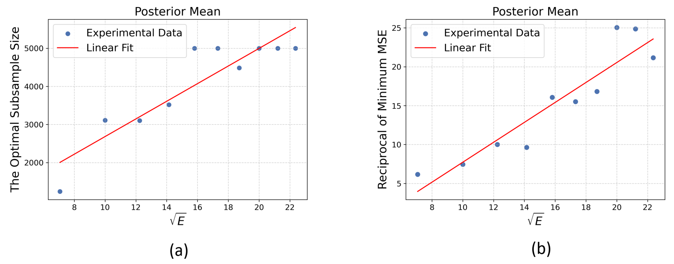
In Figure 3, the square root of the epochs and the optimal subsample size for the approximate MH algorithm, $(\sqrt{E},m^{★})$, are displayed as blue dots. These data points closely align with the fitted linear regression line. A similar phenomenon is observed for the square root of the epochs and the reciprocal of the minimum MSE $(\sqrt{E},1/{\mathrm{MSE}}^{★})$, as demonstrated in Figure 4. These observations suggest that the optimal subsample size approximately follows $m\propto E^{1/2}$ and that the minimum MSE changes as ${\mathrm{MSE}}^{★}\propto E^{-1/2}$.

As theoretically established in Section 3.2, incorporating a control variate is expected to reduce the variance of the log-likelihood ratio estimator and, consequently, the MSE of the final parameter estimates. We empirically validate this premise by applying the control variate technique to the approximate MH algorithm. The results in Figure 5 confirm this, demonstrating that the control variate-augmented algorithm substantially outperforms the exact algorithm by achieving a remarkably low MSE that remains stable as the number of epochs increases.

4.2. Bayesian Logistic Regression

The logistic regression model is a foundational method in statistical modeling and serves as a widely used benchmark. It continues to be an active area of research for various statistical challenges, such as multicollinearity [31]. In contrast, our work addresses the distinct challenge of computational efficiency for Bayesian inference with this model on large datasets.

In the logistic regression model, the data points ${\{X_i,Y_i\}}_{i=1}^n$ follow the condition that $Y_i$ is a binary outcome, where $Y_i\in \{0,1\}$. The probability that $Y_i=1$ is modeled using the sigmoid function, defined as

$$p(Y_i=1\mid X_i,\theta )={\displaystyle \frac{1}{1+e^{-{\theta }^T{X}_i}}}$$

(22)

Here, $\theta$ represents the vector of parameters to be estimated, and $X_i$ represents the feature vector for the i-th observation. The log-likelihood function is given by

$$\begin{array}{cc}\hfill \ell \left(Y\mid X_1,\dots ,X_n,\theta \right)& =\sum _{i=1}^n\ell \left(Y_i\mid X_i,\theta \right)\hfill \\ \hfill & =\sum _{i=1}^n\left((1-Y_i)log\left[1-p\left(X_i\mid \theta \right)\right]+Y_{i}logp\left(X_i\mid \theta \right)\right)\hfill \end{array}$$

(23)

For real data ${\{X_i,Y_i\}}_{i=1}^n$, we use a commonly used dataset from covtype (https://www.csie.ntu.edu.tw/~cjlin/libsvmtools/datasets/binary.html, accessed on 6 June 2024). The entire dataset contains 581,012 data points, with the original data having 54 dimensions. Among these, only the first 10 variables are quantitative, while the remaining are dummy variables. We retain only the first 10 variables as features and follow the data preprocessing method and prior distribution as outlined in [37], using the Cauchy distribution with a center vector 0 and a scale matrix $\mathbf{S}$ where $\mathbf{S}$ is a diagonal matrix with each diagonal element equal to 2.5, as the prior distribution.

In this experiment, we applied two MH schemes—an approximate algorithm with control variates (improved MH) and the exact (vanilla) MH—to obtain empirical posterior distributions and estimate the three parameters of interest specified in Equation (21). Figure 6 depicts the evolution of the MSE across epochs for each of the three estimators under both MH schemes. At each epoch, the reported MSE corresponds to the minimum value achieved over a grid of subsample sizes. The vanilla MH algorithm exhibits a clear dependence on the computational budget. Its MSE is initially high for a small number of epochs because the estimator’s variance dominates due to insufficient sampling. As the computational budget E increases, this variance-driven error gradually decreases. In contrast, the approximate MH algorithm augmented with control variates maintains a consistently low MSE across the entire range of computational budgets examined, as illustrated in Figure 6. This superior performance demonstrates the effectiveness of the control variate used in this model. The resulting variance term, ${\sigma }_{cv}$, is sufficiently small so that the overall MSE is greatly reduced and becomes less sensitive to the number of epochs E. This experiment further confirms the importance of reducing the variance of the log-likelihood ratio estimator. To further validate the robustness of our findings, we conducted an additional experiment on a second real-world dataset, HIGGS (https://archive.ics.uci.edu/dataset/280/higgs, accessed on 25 June 2025). The results were consistent with those observed on the “covtype” dataset, reaffirming the significant computational advantage of the improved approximate MH algorithm. For the sake of brevity in the main text, the detailed setup and results of this supplementary experiment are provided in Appendix B.

Beyond our control variate approach, other variance-reduction techniques may also be employed. For example, some methods incorporate ideas from stratified sampling [38,39], while others focus on designing non-uniform sampling schemes to select more informative data points [12,23].

4.3. Softmax Classification

Softmax regression is a standard method for multi-class classification problems. Its log-likelihood function is given by

$$logp(\mathbf{y}\mid \mathbf{x},\theta )=\sum _{i=1}^N\sum _{k=1}^K\mathbf{1}\{y_i=k\}log\left({\displaystyle \frac{exp\left({\theta }_k^T{\mathbf{x}}_i\right)}{{\sum }_{j=1}^{K}exp\left({\theta }_j^T{\mathbf{x}}_i\right)}}\right).$$

(24)

Estimating the posterior distribution of this model using MCMC algorithms has been explored in prior work [10]. In our experiment, we leverage the posterior to make predictions via Bayesian model averaging. Specifically, for each test point $({\mathbf{x}}^{*},y^{*})$, the predictive probability is given by the posterior predictive mean: ${\mathbb{E}}_{\pi \left(\theta \right)}\left[p(y^{*}\mid {\mathbf{x}}^{*},\theta )\right].$ We then compare the test set predictive accuracy of the model average generated by the control variate-augmented approximate MH algorithm with that produced by the exact MH algorithm. The theoretical non-identifiability of the Softmax regression model is not a confounding factor in this comparison. This is because, in our practical implementation, the shared initialization point $\widehat{\theta }$ and the tight proposal scaling (per Assumption 5) effectively confine both MCMC chains to the same local high-probability region.

We use the classic MNIST (http://yann.lecun.com/exdb/mnist/, accessed on 16 June 2024) dataset of handwritten digits for multi-class prediction. The original dataset includes images of 10 digits ranging from 0 to 9. We selected the first 5 digits in this experiment. To create a balanced dataset, we identified the smallest class and sampled an equal number of instances from the remaining classes. This resulted in a training dataset of 29,210 samples and a test set of 4900 samples. Additionally, we reduced the dimensionality of the data from 784 to 50 using Principal Component Analysis as described by [24]. In our MCMC algorithm, we employed a non-informative prior distribution.

Across all experimental settings, the approximate MH algorithm utilized only 1% of the full dataset in each iteration. For each computational budget listed in

Table 1. Prediction accuracy.

Epochs	20	30	50	100	150	200	250	300
Approximate	90.49%	90.67%	91.53%	92.27%	92.04%	92.39%	92.29%	93.14%
Vanilla	89.65%	89.88%	89.69%	90.14%	90.12%	90.31%	90.53%	90.59%

, we generated samples from both the approximate and the exact MH algorithms to estimate the predictive mean for each point in the test set. Instead of using the MSE of the predictive mean as our evaluation metric, we adopt the more intuitive measure of prediction accuracy on the test set. Prediction accuracy serves as a practical proxy for the estimator’s MSE, as a lower MSE generally corresponds to higher predictive accuracy. The final predictions are made based on the estimated probabilities, and Table 1 summarizes the comparative accuracy of both algorithms across various computational budgets.

We observe that both algorithms exhibit a clear upward trend in test set prediction accuracy as the computational budget increases, implying that the estimation error shrinks as E grows. However, for any given number of epochs, the prediction accuracy of the vanilla MH algorithm is consistently lower than that of the approximate MH algorithm. This performance gap is attributable to a dual advantage of the control variate-augmented method. The control variate effectively mitigates the bias introduced by subsampling, even with a small m. Simultaneously, for the computational budgets summarized in Table 1, a small m permits a larger number of MCMC iterations, which in turn reduces the estimator’s variance. This combined reduction in both bias and variance results in a lower MSE, which in turn leads to higher prediction accuracy than that of the exact MH algorithm.

5. Conclusions and Future Work

This study analyzes an approximate MH algorithm that estimates the log-likelihood ratio using random data subsets. Our primary contribution is a theoretical analysis of the MSE for the algorithm’s posterior estimates. We establish the optimal asymptotic scaling for the bias–variance trade-off, showing that the ideal subsample size scales with the number of computational epochs as $m^{★}=O\left(E^{1/2}\right)$, resulting in a minimal MSE that decays as ${\mathrm{MSE}}^{★}=O\left(E^{-1/2}\right)$. Furthermore, leveraging the large-sample asymptotic properties of the posterior, we deepen the analysis of the approximate MH algorithm’s convergence. We demonstrate that when an exact control variate is incorporated into the subsample-based estimator, the approximate MH algorithm can be asymptotically more efficient than the standard MH method under ideal conditions. From an experimental perspective that accounts for both statistical and computational complexity, the two algorithms exhibit distinct behaviors: the MSE of the exact algorithm is large with fewer epochs and gradually decreases as the number of epochs grows. In contrast, the MSE of the approximate algorithm is substantially lower than that of the exact algorithm and remains stable at a low value, largely insensitive to the number of epochs.

To improve performance in high-dimensional settings, future research should move beyond inefficient random walk proposals. We suggest a theoretical analysis of approximate MCMC algorithms coupled with informed, gradient-based proposals, like the Metropolis-Adjusted Langevin Algorithm (MALA) and Hamiltonian Monte Carlo (HMC), to significantly boost sampling efficiency. A key theoretical challenge would be to analyze the impact of the additional noise from gradient estimation and to derive the joint optimal scaling laws for the expanded set of tuning parameters, which includes both the subsample size and algorithm-specific parameters such as step size.

References

1. Bardenet, R.; Doucet, A.; Holmes, C. On Markov chain Monte Carlo methods for tall data. J. Mach. Learn. Res. 2017, 18, 1–43. [Google Scholar]
2. Nemeth, C.; Fearnhead, P. Stochastic gradient markov chain monte carlo. J. Am. Stat. Assoc. 2021, 116, 433–450. [Google Scholar] [CrossRef]
3. Neiswanger, W.; Wang, C.; Xing, E. Asymptotically exact, embarrassingly parallel MCMC. In Proceedings of the 30th Conference on Uncertainty in Artificial Intelligence (UAI’14), Quebec City, QC, Canada, 23–27 July 2014; pp. 623–632. [Google Scholar]
4. Williamson, S.; Dubey, A.; Xing, E. Parallel Markov chain Monte Carlo for nonparametric mixture models. In Proceedings of the 30th International Conference on Machine Learning, PMLR, Atlanta, GA, USA, 16–21 June 2013; pp. 98–106. [Google Scholar]
5. Angelino, E.; Kohler, E.; Waterland, A.; Seltzer, M.; Adams, R.P. Accelerating MCMC via parallel predictive prefetching. In Proceedings of the 30th Conference on Uncertainty in Artificial Intelligence (UAI’14), Quebec City, QC, Canada, 23–27 July 2014; pp. 22–31. [Google Scholar]
6. Glatt-Holtz, N.E.; Holbrook, A.J.; Krometis, J.A.; Mondaini, C.F. Parallel MCMC algorithms: Theoretical foundations, algorithm design, case studies. Trans. Math. Its Appl. 2024, 8, tnae004. [Google Scholar] [CrossRef]
7. Mesquita, D.; Blomstedt, P.; Kaski, S. Embarrassingly parallel MCMC using deep invertible transformations. In Proceedings of the 35th Uncertainty in Artificial Intelligence, PMLR, Tel Aviv, Israel, 22–25 July 2020; pp. 1244–1252. [Google Scholar]
8. Wang, T.; Wang, G. Unbiased Multilevel Monte Carlo methods for intractable distributions: MLMC meets MCMC. J. Mach. Learn. Res. 2023, 24, 1–40. [Google Scholar]
9. Vyner, C.; Nemeth, C.; Sherlock, C. SwISS: A scalable Markov chain Monte Carlo divide-and-conquer strategy. Stat 2023, 12, e523. [Google Scholar] [CrossRef]
10. Maclaurin, D.; Adams, R.P. Firefly Monte Carlo: Exact MCMC with subsets of data. In Proceedings of the 30th Conference on Uncertainty in Artificial Intelligence (UAI’14), Quebec City, QC, Canada, 23–27 July 2014; pp. 543–552. [Google Scholar]
11. Zhang, R.; Cooper, A.F.; De Sa, C.M. Asymptotically optimal exact minibatch metropolis-hastings. Adv. Neural Inf. Process. Syst. 2020, 33, 19500–19510. [Google Scholar]
12. Putcha, S.; Nemeth, C.; Fearnhead, P. Preferential Subsampling for Stochastic Gradient Langevin Dynamics. In Proceedings of the 26th International Conference on Artificial Intelligence and Statistics, PMLR, Valencia, Spain, 25–27 April 2023; pp. 8837–8856. [Google Scholar]
13. Wu, T.Y.; Rachel Wang, Y.; Wong, W.H. Mini-batch Metropolis–Hastings with reversible SGLD proposal. J. Am. Stat. Assoc. 2022, 117, 386–394. [Google Scholar] [CrossRef]
14. Pollock, M.; Fearnhead, P.; Johansen, A.M.; Roberts, G.O. Quasi-stationary Monte Carlo and the ScaLE algorithm. J. R. Stat. Soc. Ser. B Stat. Methodol. 2020, 82, 1167–1221. [Google Scholar] [CrossRef]
15. Lykkegaard, M.B.; Dodwell, T.J.; Fox, C.; Mingas, G.; Scheichl, R. Multilevel delayed acceptance MCMC. SIAM/ASA J. Uncertain. Quantif. 2023, 11, 1–30. [Google Scholar] [CrossRef]
16. Maire, F.; Friel, N.; Alquier, P. Informed sub-sampling MCMC: Approximate Bayesian inference for large datasets. Stat. Comput. 2019, 29, 449–482. [Google Scholar] [CrossRef]
17. Quiroz, M.; Kohn, R.; Villani, M.; Tran, M.N. Speeding up MCMC by efficient data subsampling. J. Am. Stat. Assoc. 2018, 114, 831–843. [Google Scholar] [CrossRef]
18. Levi, E.; Craiu, R.V. Finding our way in the dark: Approximate MCMC for approximate Bayesian methods. Bayesian Anal. 2022, 17, 193–221. [Google Scholar] [CrossRef]
19. Hermans, J.; Begy, V.; Louppe, G. Likelihood-free mcmc with amortized approximate ratio estimators. In Proceedings of the 37th International Conference on Machine Learning, PMLR, Virtual, 13–18 July 2020; pp. 4239–4248. [Google Scholar]
20. Conrad, P.R.; Marzouk, Y.M.; Pillai, N.S.; Smith, A. Accelerating asymptotically exact MCMC for computationally intensive models via local approximations. J. Am. Stat. Assoc. 2016, 111, 1591–1607. [Google Scholar] [CrossRef]
21. Sherlock, C.; Thiery, A.H.; Roberts, G.O.; Rosenthal, J.S. On the efficiency of pseudo-marginal random walk Metropolis algorithms. Ann. Stat. 2015, 43, 238–275. [Google Scholar] [CrossRef]
22. Alquier, P.; Friel, N.; Everitt, R.; Boland, A. Noisy Monte Carlo: Convergence of Markov chains with approximate transition kernels. Stat. Comput. 2016, 26, 29–47. [Google Scholar] [CrossRef]
23. Hu, G.; Wang, H. Most likely optimal subsampled Markov chain Monte Carlo. J. Syst. Sci. Complex. 2021, 34, 1121–1134. [Google Scholar] [CrossRef]
24. Korattikara, A.; Chen, Y.; Welling, M. Austerity in MCMC land: Cutting the Metropolis-Hastings budget. In Proceedings of the 31st International Conference on Machine Learning, PMLR, Beijing, China, 21–26 June 2014; pp. 181–189. [Google Scholar]
25. Bardenet, R.; Doucet, A.; Holmes, C. Towards scaling up Markov chain Monte Carlo: An adaptive subsampling approach. In Proceedings of the 31st International Conference on Machine Learning, PMLR, Beijing, China, 21–26 June 2014; pp. 405–413. [Google Scholar]
26. Pitt, M.K.; dos Santos Silva, R.; Giordani, P.; Kohn, R. On some properties of Markov chain Monte Carlo simulation methods based on the particle filter. J. Econom. 2012, 171, 134–151. [Google Scholar] [CrossRef]
27. Doucet, A.; Pitt, M.K.; Deligiannidis, G.; Kohn, R. Efficient implementation of Markov chain Monte Carlo when using an unbiased likelihood estimator. Biometrika 2015, 102, 295–313. [Google Scholar] [CrossRef]
28. Jacob, P.E.; Thiery, A.H. On nonnegative unbiased estimators. Ann. Statist. 2015, 43, 769–784. [Google Scholar] [CrossRef]
29. Johndrow, J.E.; Mattingly, J.C.; Mukherjee, S.; Dunson, D. Optimal approximating Markov chains for Bayesian inference. arXiv 2015, arXiv:1508.03387. [Google Scholar]
30. Van der Vaart, A.W. Asymptotic Statistics; Cambridge University Press: Cambridge, UK, 2000; Volume 3. [Google Scholar]
31. Roozbeh, M. Optimal ridge estimation in the restricted logistic semiparametric regression models using generalized cross-validation. J. Appl. Stat. 2025, 1–20. [Google Scholar] [CrossRef]
32. Malinovsky, G.; Horváth, S.; Burlachenko, K.; Richtárik, P. Federated learning with regularized client participation. In Proceedings of the Workshop of Federated Learning and Analytics in Practice, Colocated with 40th International Conference on Machine Learning, Honolulu, HI, USA, 23–29 July 2023. [Google Scholar]
33. Fishman, G.S. Monte Carlo: Concepts, Algorithms, and Applications; Springer: New York, NY, USA, 1996. [Google Scholar]
34. Gelman, A.; Gilks, W.R.; Roberts, G.O. Weak convergence and optimal scaling of random walk Metropolis algorithms. Ann. Appl. Probab. 1997, 7, 110–120. [Google Scholar] [CrossRef]
35. Roberts, G.O.; Rosenthal, J.S. Optimal scaling for various Metropolis-Hastings algorithms. Stat. Sci. 2001, 16, 351–367. [Google Scholar] [CrossRef]
36. Chib, S.; Greenberg, E. Understanding the metropolis-hastings algorithm. Am. Stat. 1995, 49, 327–335. [Google Scholar] [CrossRef]
37. Gelman, A.; Jakulin, A.; Pittau, M.G.; Su, Y.S. A weakly informative default prior distribution for logistic and other regression models. Ann. Appl. Stat. 2008, 2, 1360–1383. [Google Scholar] [CrossRef]
38. Sen, D.; Sachs, M.; Lu, J.; Dunson, D.B. Efficient posterior sampling for high-dimensional imbalanced logistic regression. Biometrika 2020, 107, 1005–1012. [Google Scholar] [CrossRef]
39. Bou-Rabee, N.; Marsden, M. Unadjusted Hamiltonian MCMC with stratified Monte Carlo time integration. Ann. Appl. Probab. 2025, 35, 360–392. [Google Scholar] [CrossRef]
Figure 1. MSE as a function of the subsample proportion for different numbers of training epochs (E). Each subplot corresponds to a fixed number of epochs: E = 50 (left), E = 350 (center), and E = 500 (right). The blue bars show the empirical MSE, the red line is a smoothed curve illustrating the trend, and the blue dot marks the minimum observed MSE for that epoch count. This figure illustrates the core bias–variance trade-off: for any fixed computational budget, there is an optimal subsample size that minimizes the estimation error.
Mathematics 13 03395 g001
Figure 2. Empirical validation of the theoretical asymptotic scaling laws. The plots show the optimal algorithm properties aggregated from experiments across a range of epoch counts (E). Subplot (a) displays the optimal subsample size ( m * ) versus E , while subplot (b) shows the reciprocal of the minimum MSE ( 1 / MSE ) versus E . The strong linear relationships observed in both plots provide empirical confirmation for the two key theoretical scaling laws derived in our work: m * E and 1 / MSE E .
Mathematics 13 03395 g002
Figure 3. Empirical validation of the optimal subsample size scaling law. Each subplot displays the optimal subsample size ( m ) plotted against the square root of the number of epochs ( E ) for three different posterior mean estimators ( μ 1 , μ 2 , μ 3 ) in the AR(2) model experiment. The strong linear relationship across all three cases provides empirical support for the first theoretical scaling law, m E .
Mathematics 13 03395 g003
Figure 4. Empirical validation of the minimal MSE scaling law. Each subplot displays the reciprocal of the minimum MSE ( 1 / MSE ) ), a measure of statistical efficiency, plotted against the square root of the number of epochs ( E ) for the three estimators in the AR(2) model experiment. The strong linear fits confirm the second theoretical scaling law, demonstrating that the statistical efficiency scales linearly with the square root of the computational budget, i.e., 1 / MSE E .
Mathematics 13 03395 g004
Figure 5. Convergence of MSE for the improved MH and vanilla MH algorithms in an AR(2) model. The MSE is plotted as a function of epochs for three different posterior mean estimators ( μ 1 , μ 2 , μ 3 ). The plots show that the vanilla MH algorithm’s MSE (dashed orange curve) gradually decreases with more epochs, while the improved MH algorithm (solid blue curve) converges almost instantly to a near-zero MSE.
Mathematics 13 03395 g005
Figure 6. Comparison of mean squared error (MSE) convergence for the improved MH and standard vanilla MH algorithms in a Bayesian logistic regression model. Each subplot shows the MSE for a different posterior mean estimator ( μ 1 , μ 2 , μ 3 ), plotted as a function of the number of epochs. The results demonstrate that the improved MH method (solid green curve) consistently achieves a near-zero MSE almost immediately, while the vanilla MH method (dashed purple curve) requires significantly more epochs to converge to a higher final error.
Mathematics 13 03395 g006