Abstract
This paper advances beyond adversarial neural network methods by considering whether the underlying mathematics of neural networks contains inherent properties that can be exploited to fool neural networks. In broad terms, this paper will consider a neural network to be composed of a series of linear transformations between layers of the network, interspersed with nonlinear stages that serve to compress outliers. The input layer of the network is typically extremely high-dimensional, yet the final classification is in a space of a much lower dimension. This dimensional reduction leads to the existence of a null space, and this paper will explore how that can be exploited. Specifically, this paper explores the null space properties of neural networks by extending the null space definition from linear to nonlinear maps and discussing the presence of a null space in neural networks. The null space of a neural network characterizes the component of input data that makes no contribution to the final prediction so that we can exploit it to trick the neural network. One application described here leads to a method of image steganography. Through experiments on image data sets such as MNIST, it has been shown that the null space components can be used to force the neural network to choose a selected hidden image class, even though the overall image can be made to look like a completely different image. The paper concludes with comparisons between what a human viewer would see and the part of the image that the neural network is actually using to make predictions, hence showing that what the neural network “sees” is completely different than what we would expect.
MSC:
68T07
1. Introduction
Despite their remarkable success in various tasks, neural networks (NNs) can sometimes behave in unexpectedly fragile ways, particularly in image recognition. One well-known problem is the existence of adversarial examples, where even small, carefully crafted perturbations to the input can lead to incorrect outputs [1,2]. While adversarial examples highlight an important class of vulnerabilities, they are not the only cause of unreliability. Such behaviors are not merely the result of noisy inputs or training data limitations but may reflect deeper issues rooted in the architecture of the neural networks. In this work, we take a different perspective to examine a structural property of neural networks, namely their null space, as a potential source of fragility.
Many existing studies attribute the vulnerability of neural networks to input-level manipulations. In 2014, Szegedy et al. [3] first discovered an intriguing weakness of deep neural networks. They showed that neural networks for image classification can be easily fooled by small perturbations. Following this observation, numerous studies have been carried out to find different ways to generate adversarial examples (see, for example, [2,4,5,6]). It is observed that adversarial examples have good transferability across models, which suggests that the existence of adversarial examples is also a property of data sets [7]. Thus, adversarial examples are not restricted to the given model.
Unlike the adversarial examples, our study focuses on a structural property of neural networks: the null space of neural networks. The null space is a well-established concept in linear algebra, but its connection to neural networks may not be obvious. If one were to consider a standard neural network from the perspective of a mathematician, the input can be considered a vector, generally in a high-dimensional space. Considering Figure 1, each entry in the input vector is placed in an open circle in the input layer. If we ignore for the moment the unitary node indicated by the 1 at the bottom of the first layer, the weights are multiplied by the entries in the input vector to produce the intermediate values , where at the nodes in the middle layer. Hence, the mathematical structure is basically a matrix multiplication of a weight matrix W times the input vector , so the presence of a null space associated with the weight matrix is very possible. Further, in the case of an NN, the known information is in the input vector and the weight matrix is to be determined via the training process. Note that the number of degrees of freedom in W is much greater than the dimension of the input vector; thus the training process can lead to underdetermined systems and high-dimensional null spaces.
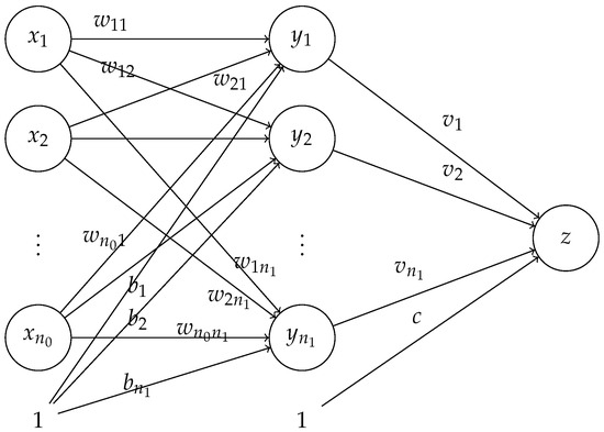
Figure 1.
Basic structure of a fully connected neural network.
In the simplest examples of NNs, the transformation from one layer to the next may be a linear transformation, but a bias term, as indicated by the unitary node labeled 1 at the bottom of the input layer, is usually introduced, which then converts the transformations into affine transformations. The affine form will introduce some complications, and this paper will explore the impact of this on the null space characteristics of the linear transformation component of NNs. When all of the layers are considered, along with the activation functions, we say that we have a fully connected neural network (FCNN) with nodes in the first layer, nodes in the second layer, and so on. This FCNN is also referred to as an -FCNN. Finally, it should be mentioned that a nonlinear activation function is usually applied to the data in an intermediate layer, such as a sigmoid function or ReLU function, but these functions can be thought of as a compressing or compactifying function that diminishes the impact of outlier results or, in the case of ReLU, negative-valued intermediate results. While these nonlinear activation functions can obfuscate the impact of the null space effects, this paper will separate out the stages to show that the null space properties, extended to consider the nonlinear effects, can be used to fool the NN and cause it to give unexpected classification results. A detailed analysis will be given in Section 2.
As a primary goal, we discuss how the null space of a neural network affects classification outcomes, revealing it to be a critical factor that may inherently limit a model’s ability to make reliable predictions. The approach takes advantage of the (nonlinear) null space properties of the neural network and generates examples to fool the neural network by adding a large difference to images without changing the predictions. More importantly, to the naked eye, the large differences will look like completely different objects than those that will be recognized by the neural network, achieved via image steganography. Considered from a broader perspective, only a few studies have analyzed the null space properties of neural network functions. Cook et al. [8] integrated the null space analysis on weight matrices with the loss function to detect out-of-distribution inputs rather than analyzing the reliability of NN predictions. Rezaei et al. [9] used the null space of the last layer weight matrix to quantify overfitting. Beyond these, some studies have investigated the null space structure of the parameter space. Sonoda et al. [10] showed that the parameter spaces of overparameterized NNs inherently contain null components that do not affect training loss but may impact generalization. In addition, a few studies have worked on the null space associated with the input data itself [11,12,13].
However, there is still a lack of understanding regarding the global effects of null space properties for NNs. In this study, inspired by the null space of linear maps, we introduce the concept of a null space for nonlinear maps and discuss how the null space applies to fully connected neural networks (FCNNs). We show how the null space is generally an intrinsic property of NNs. Further, in most cases, once the NN’s architecture is determined, the dimension of the null space of the NN is also determined. To illustrate this in concrete terms, we use null space-based methods to fool an image recognition NN, demonstrating an application of image steganography.
Image steganography is a technique to hide an image inside another image [14,15]. Traditional image steganography methods can be categorized into two main types: methods operating in the spatial domain [16] and the transform domain [17]. Among methods operating in the transform domain, discrete orthogonal moment transforms have been widely used in image analysis and image steganography [18,19,20,21,22]. In addition to traditional steganography methods, approaches based on NNs have also been employed for image steganography, using several different approaches [23,24,25,26,27,28,29,30,31]. In this paper, inspired by the null space analysis of NNs, we propose a null space-based method for image steganography. Our approach shares some similarity with discrete orthogonal moment-based steganography, as both methods decompose images with respect to a chosen basis. However, while moment methods rely on polynomial bases (e.g., Tchebichef, Krawtchouk), our method employs basis vectors from the null space of a neural network. In addition, although conceptually related to other steganographic methods, the null space-based method presented in this paper provides new degrees of freedom and a clear process for creating steganographic images for NNs. The main goal is to hide an image and recognize the correct class of the hidden image while presenting to the (human) viewer an image that is completely different to the hidden image that will be recognized by the NN.
In summary, the main contributions of this paper are as follows:
- We introduce a novel perspective on NN reliability by analyzing the role of the null space structure for the NN and showing that its dimension is architecture-dependent.
- We propose a null space-based steganographic method that generates visually different images while hiding images that are recognized with high certainty by the model.
The rest of this paper is organized as follows: Section 2 introduces the (nonlinear) null space of NNs. Inspired by null space analysis, an image steganography method based on the null space of FCNNs is introduced in Section 3. Section 4 presents a series of experiments on different image data sets. In Section 5, we offer some discussion and conclusions about the advantages and limitations of the null space method and the differences between the null space image steganography method and adversarial examples. Additionally, more examples are presented to emphasize that what the NN is seeing and using to make classification decisions is not what we humans might perceive it to be seeing.
2. Methodology and Theory
In this section, we introduce the null space of nonlinear maps and discuss the null space of neural networks (NNs). In order to keep the flow of ideas consistent, detailed proofs will be placed in the appendix.
2.1. Null Space of Linear and Nonlinear Maps
In linear algebra, the null space of an matrix A is and is a subspace of . Consider a linear map with nontrivial. By the definition of a null space, it is not difficult to see that for any and , . That is, adding any vector in to any input will not change the output since the transformation is a linear map.
In most cases, null space in nonlinear maps is not defined as described above. The set for a nonlinear map is not a subspace of . Moreover, the property of linearity does not hold for the nonlinear map f. Although we can still find the set , the property is no longer true for all . To preserve this useful property, the concept of null space can be adapted to nonlinear maps by identifying a set of vectors that satisfy the condition for any :
Definition 1
(Null space of a nonlinear map). The null space of a nonlinear map , denoted as , is the set of all vectors in which, by adding these vectors to any input, the image under the map, or output, will not change:
When this definition is applied to linear maps, it is equivalent to the null space concept in linear algebra. However, for the purposes of this paper, we will use the term “null space” in a broader sense, extending its application to include affine maps, nonlinear maps, etc. Similarly to the null space in linear algebra, is a subspace of (Proposition A1). Furthermore, as demonstrated in Proposition A2, all the vectors in are mapped to a single point by f. More specifically, for any . Further properties about null spaces of nonlinear maps are provided in Appendix B. One difference between null spaces of linear and nonlinear maps is that a nonlinear map will not always map null space vectors to zeros.
The definition of the null space for nonlinear maps is straightforward. However, in practice, it is difficult to find a null space explicitly by following this definition. Next, we will introduce an alternative yet equivalent definition for the null space of nonlinear maps, which provides a more accessible way with which to find the null space of a nonlinear map.
To begin with, given a nonlinear map , let us consider the subspaces of . Suppose f has a decomposition; then, f can be expressed as the composition of two functions and is linear. It follows that is a subspace of . This is straightforward to see, since for any , holds for every , and so . Therefore, we now have a method to find a subspace of . Hence, we define a partial null space as follows:
Definition 2
(Partial null space of a map). Given a nonlinear map, . If f has a decomposition , where is a linear map, then the null space of is defined as a partial null space of f (given by ). We denote it as .
Then, the question of how to find the null space with partial null spaces and the decomposition of maps remains. In the following lemmas, we present some results regarding partial null spaces and the null space of a nonlinear map. Detailed proofs are provided in Appendix B.
Lemma 1.
Let be a nonlinear map. Every partial null space is a subspace of , .
Lemma 2.
For every nonlinear map , there exists a decomposition , where is a linear map such that , i.e., the partial null space given by is equal to .
Note that is not always true for any arbitrary decomposition . In the following corollary, we further discuss the conditions under which this equation holds.
Corollary 1.
Let be a nonlinear map. The null space of f is the largest partial null space of f. That is, if , is a linear map, and has the largest dimension among all decompositions of f.
Directly from Lemmas 1 and 2, Corollary 1 gives an equivalent definition of in terms of its partial null space. Consequently, instead of searching for all possible vectors that satisfy Equation (1), we have turned the null space problem into a problem of finding a decomposition of f that yields the largest partial null space.
2.2. Null Space of Fully Connected Neural Networks
Consider a fully connected neural network , where denotes the number of hidden layers of f, with representing widths of the hidden layers, i.e., the number of nodes in each hidden layer. are the input and output dimensions, respectively. f is called a layer fully connected neural network (FCNN). In this paper, we refer to this FCNN architecture as a FCNN.
As shown in Figure 2, assume the input values are and the activation functions are denoted by ; then the output of the kth neuron in the jth layer is given by and the outputs of the jth layer can be written in a compact matrix form The function represented by this neural network is
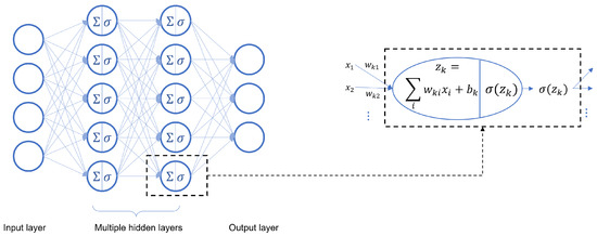
Figure 2.
Architecture of a fully connected neural network.
Define a sequence of linear and affine transformations as for , respectively. The function of FCNN f can also be represented by a composition of maps:
Common activation functions include sigmoid activation function and Rectified Linear Unit (ReLU). We refer to the -FCNN with ReLU activation as a -ReLU NN.
According to Corollary 1, we can conduct null space analysis on FCNNs using the composite function form (Equation (2)). An FCNN can be naturally decomposed into two parts, and , where is linear. Thus, is a partial null space of FCNN f which, in most cases, is also the null space .
As will be shown in Section 3, input images can be decomposed into null space and non-null space components, which can be used to fool the neural networks in an image steganography application.
2.3. Null Space of Convolutional Neural Networks
Similarly, a convolutional neural network (CNN) can also be represented by the composition of maps. Instead of having only affine transformations and activation functions, the early layers of a CNN allow two additional types of computation: convolution, denoted as C, and pooling, denoted as S. To determine the null space of a CNN f, we can first decompose f into the composition of maps . So, in most cases, the first convolution operation C is the maximum linear map of f, and .
The null space of a CNN is significantly more complex than an FCNN. In this paper, we will only give an overview of the null space analysis for CNN in a simple case. Consider the case when the input image of a CNN only has one channel, for example the grayscale number images in the MNIST data set (a color image typically has three channels).
A typical convolutional layer in a CNN comprises multiple kernels. To find the null space of the entire convolutional layer , we can initially determine the null space of a single kernel corresponding to one convolution operation. As shown in Appendix C, given one kernel, if the convolution operation keeps the output image with the same dimensions as the input image (same padding), then in most cases. If the output image of the first convolution operation has fewer dimensions than the input image (valid padding), can be nontrivial. According to Lemma A1, in most cases, the null space of a given kernel has a dimension that is equal to the difference between the dimensions of the input and output image. For example, given a image and a kernel, the dimension of the null space of this convolution operation is in most cases.
Assume that the first convolutional layer C has n kernels ; then . For instance, if the input is a image and the first convolutional layer has six kernels, then the null space of the CNN is the intersection of six dimensional subspaces of . The likelihood of there being a non-trivial intersection between 109-dimensional subspaces of a 784-dimensional space is low, but care must be taken when designing the kernels.
Compared to FCNNs, CNNs can achieve a trivial null space with fewer unknown parameters in the first weight matrix and perhaps greater robustness.
3. Photo Steganography Based on the Null Space of a Neural Network
In considering the task of hiding secret information inside another image, a natural idea emerges from our previous discussions on the null space properties of FCNNs. To this end, in this section we propose a method for creating steganographic images, referred to as “stego images”, to fool FCNNs and pass on secret classification information.
In terms of a pre-trained FCNN f, for any input image X, the FCNN f gives a decomposition,
where is the projection of X onto the null space of f and is the orthogonal complement that determines the prediction. Since , the output depends solely on ; that is, . This decomposition provides the idea for controlling the predicted label/classification independently of the image’s appearance.
Consider two images H and C: H is the hidden image which carries the secret label. C is the cover image which determines the visual appearance. Our goal is to pass a new image S that visually looks like C but secretly hides the classification information of H, i.e., which is classified the same as the hidden image by f. This can be achieved by decomposing both H and C with respect to the null space : the null space projections, denoted by and , which lie in the null space and do not affect the prediction; and the orthogonal complements, denoted by and , which contribute to the output of f. Importantly, this method does not involve retraining the network; instead, the null space is computed directly from the first layer of a pre-trained neural network f. By combining the null space projection of C, denoted by , with the prediction-relevant component of H, denoted by , we construct
so that S appears similar to C but satisfies if the f is trained on grayscale images to correctly classify the scaled inputs, such as for . The pseudocode of the proposed image steganography method is provided in Appendix A.
Figure 3 provides a visualization of the whole process. We consider a data set , where are grayscale images normalized to the range and are class labels. First, a fully connected ReLU network f is trained on both the original images and their rescaled versions , where , to create “headroom” for linear combinations. Then, the null space is obtained by computing the singular value decomposition (SVD) of the first hidden layer weight matrix and extracting the columns of V associated with zero singular values, which form an orthonormal basis for the null space . These columns form the matrix . If H and C are column vectors in the form of neural network inputs, we compute and as follows:
where and give the coefficients (dot products) of H and C along the null space basis vectors, respectively. Multiplying by reconstructs the projection within the null space. Thus, is composed only of null space vectors, while has all null space components removed. Finally, we construct the stego image . Note that the resulting stego image S must remain within the normalized range , consistent with the range of the neural network inputs. This condition constrains the choice of and : cannot be too large (otherwise some entries of S may fall outside ) or too small (otherwise the hidden component becomes too weak to carry sufficient information from the hidden image). Also, guaranteeing the visual quality of the cover image requires to be as large as possible.
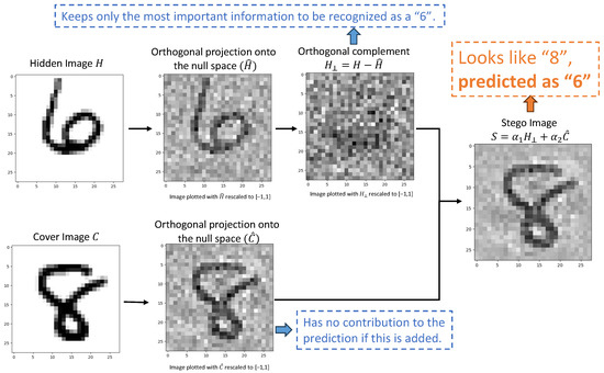
Figure 3.
An example of creating a steganographic image with the null space of an ReLU NN. For a given neural network, if we combine the null space component of the cover image with the orthogonal complement component of the hidden image, we can obtain a steganographic image that visually resembles the cover image but is classified the same as the hidden image. In this example, the steganographic image appears as the number 8, similarly to the cover image, but it is classified as a 6 because of the hidden image. Note that are not rescaled in the algorithm. The rescaling to [−1, 1] shown here is for visualization purposes only, as intermediate values may fall outside of this range and cannot be directly rendered.
In this example, the network classifies S as the digit eight based on the hidden image H while ignoring the visual features of the cover image C. So, for the example in Figure 3, the stego image looks like an “8”, but when presented to the NN, it is classified as a “6”.
In the next section, we will show experiments using the MNIST, Fashion-MNIST (FMNIST), and Extended MNIST (EMNIST) data sets. For simplification, we present experiment results using . Other values of may also be used as long as the stego image remains within the range . Further discussion on the choice of parameters and can be found in Appendix D.
4. Experimental Results
All experiments presented in this section were implemented in TensorFlow. The data sets used in these experiments include MNIST [32], Fashion-MNIST [33], Extended MNIST (EMNIST) [34], and CIFAR-10 [35].
4.1. Hide the Digits
In this section, we use the MNIST data set to conduct experiments in image steganography. For these experiments, we trained a (784, 32, 16, 10) − ReLU NN, i.e., the ReLU NN has images as the input vector in length, 32 nodes in the first hidden layer, 16 nodes in the second hidden layer, and 10 nodes in the output layer. The training was based on an expanded image training data set that included the original data set and the data set rescaled with , with a prediction accuracy of on the original training data. For the original training data correctly predicted, the average confidence level is . When evaluated on the rescaled training data, this ReLU NN maintained a high prediction accuracy of with an average confidence of on correctly predicted data. Expanding the data set to include the rescaled training data slightly reduced the training accuracy; the accuracy remains high and still provides a large pool of correctly classified images for constructing steganographic images. Notably, this ReLU NN has a 752-dimensional null space. This large null space plays a crucial role in the steganographic capabilities of the network.
We then filter out only the correctly predicted images to create a new data set. This data set comprises a total of 50,000 images, with each class having 5000 examples. The (784, 32, 16, 10) − ReLU NN can correctly predict both original and rescaled data from this new data set. The main purpose of this process is to ensure that for any chosen hidden image H from the new data set, feeding into the ReLU NN does not create scaling issues and yields a correct classification. Next, we will show some representative results with stego images produced by , where can be chosen in the range of and is generally set to around .
Figure 4 and Figure 5 present stego images generated using the images from the new data set. For each set of three images, the first is the cover image, the second is the hidden image, and the third, the stego image, combines parts of the cover and the hidden image. Additionally, Figure 4 annotates the combination weights of stego images and the predictions and their corresponding confidence levels. In each case, the ReLU NN predicts the hidden digit with high confidence.
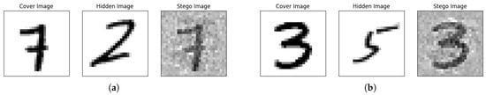
Figure 4.
Examples of steganographic images with the MNIST data set. (a) The cover image is predicted ro be 7 with a confidence of nearly 100%. The hidden image is predicted to be 2 with a confidence of nearly 100%. The stego image, , is predicted to be 2 with a confidence level of 99.9%. (b) The cover image is predicted to be 3 with a confidence of nearly 100%. The hidden image is predicted to be 5 with a confidence of nearly 100%. The stego image, , is predicted to be 5 with a confidence level of 99.9%.
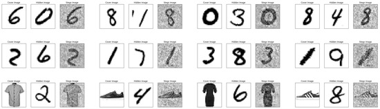
Figure 5.
More examples on the MNIST data set. For each set of three images, the stego image is the combination of the null space part of the cover image and the orthogonal complement part of the hidden image. Thus, the stego image is visually similar to the cover image but is classified based on the hidden image.
As shown in the figures, we can barely see the hidden digits in the stego images, which have patterns extremely similar to the cover images, even if the cover image is from another data set. However, these stego images are not predicted to be in the same classes as the cover images; rather, they are identified as the hidden images with high confidence. The cover image’s portion within the stego image falls entirely in the null space of the ReLU NN, giving the stego image a visible pattern that resembles the cover image (plus some noise-like structure) but makes no contribution to the prediction with the ReLU NN. On the other hand, the part of the hidden image included in the stego image appears as noise (as shown in Figure 3), but it is this portion that carries the most important information for prediction with the ReLU NN.
4.2. Results on Other Data Sets
This proposed image steganography method is general and can be applied to any image data set. In addition to the MNIST data set, we also applied our method to other image data sets: FMNIST, EMNIST, and CIFAR-10.
For the FMNIST data set, we trained a -ReLU NN with a 752-dimensional null space. To generate stego images, we first created a new data set comprising both the correctly predicted original and rescaled images (also scaled by a factor of 0.2). This new data set has an average confidence of for the original images and for the rescaled images. Examples of stego images created from the new data set are shown in Figure 6 and Figure 7.
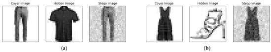
Figure 6.
Examples of steganographic images with the FMNIST data set. (a) The cover image is predicted to be “Trouser” with a confidence of nearly 100%. The hidden image is predicted to be “Shirt” with a confidence of nearly 100%. The stego image, , is predicted to be “Shirt” with a confidence level of 86.4%. (b) The cover image is predicted to be “Dress” with a confidence of nearly 100%. The hidden image is predicted to be “Sandal” with a confidence of nearly 100%. The stego image, , is predicted to be “Sandal” with confidence of nearly 100%.
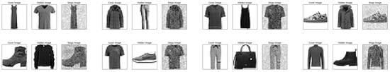
Figure 7.
More examples on the FMNIST data set.
Similarly, as expected, the stego images have the look of cover images (as seen in the first column) but are recognized as the same categories as their corresponding hidden images (shown in the second column) with high confidence.
To continue this investigation, we also perform experiments on the EMNIST Balanced data set (Figure 8) and CIFAR-10 data set (Figure 9), where the same technique works. The figures suggest that the null space-based image steganography method is also applicable to more complicated and colorful images. To guarantee the capability of concealing an image within any chosen cover image, we can train a neural network model with a sufficiently large null space. As observed in the experiments, when simple digit or letter images are used as cover images, their null space components tend to preserve most of their visual information under projection, while more complex and colorful images, such as the images in the CIFAR-10 data set, may appear more “noisy” after being projected onto the null space, therefore requiring a larger null space to maintain visual fidelity.

Figure 8.
More examples on the EMNIST data set.

Figure 9.
More examples on the CIFAR-10 data set.
4.3. Analysis of Reduced Confidence in Stego Images
While most stego images constructed by our method are classified the same as the hidden image with nearly 100% confidence, in a few cases, a reduced confidence is observed. In this regard, it is worthwhile to look at these outliers.
One such outlier result is shown in Figure 6a. While the original hidden image H is predicted to be a “shirt” with confidence close to 1, the stego image is predicted to be a “shirt” with a lower confidence of . The reduced confidence level is caused by the rescaled hidden image. According to the null space method, the prediction and confidence level for the stego image S should align with those for and, consequently, . Consistent with this analysis, the rescaled hidden image is also predicted to be “shirt” with 86.4% confidence. Therefore, the confidence drop reflects the effect of rescaling rather than a limitation of the null space method.
Unlike the experiment with the MNIST data set, it is more common to see lower confidence stego image examples in the experiment with the FMNIST data set. In Figure 10, we compare the original hidden image H and rescaled hidden image in Figure 6a. For the rescaled image , the NN gave a reduced confidence of for the correct prediction of “shirt”, but it also predicted the related category of “T-shirt/Top” with a confidence of . As shown in Figure 10, the rescaling operation reduces contrast and leads to the loss of some visual details, which causes lower confidence. For instance, the buttons and collar cannot be clearly observed in the rescaled image, so it is also more likely to be identified as a “T-shirt/Top”.
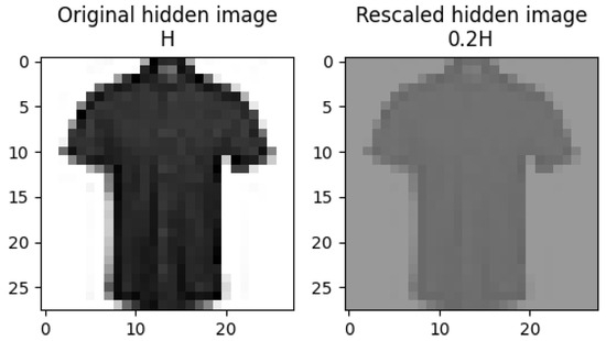
Figure 10.
Original and rescaled images.
Therefore, the achievement of high confidence in steganographic images depends on having “good” hidden images with high confidence on both original and rescaled data. Essentially, the prediction confidence level of the hidden images will be no better than the prediction confidence of the original images after rescaling has been applied.
5. Discussions and Conclusions
This study discusses the fundamental role of null space in NNs, the reliability issues it may introduce, and how it can be exploited. The null space is a structural property inherent to the architecture of the NN itself, which is independent of the input data. By extending the null space concept from linear transformations to complex NN architectures, we demonstrate that this hidden structure can lead to serious reliability concerns. More specifically, if a neural network has a high-dimensional null space, it remains vulnerable, no matter how well it is trained, because one can always construct inputs to fool the model. In this regard, CNNs tend to be more robust than FCNNs from the null space perspective, as their architectures typically induce a much smaller or even trivial null space. However, the null space property can also be used for beneficial applications, including but not limited to image steganography.
These findings have implications for model interpretability and reliability. The following discussion elaborates on what the NN actually "sees" and broader concerns like reliability in AI systems.
5.1. What We See and What NNs See
From the analysis and experimental results presented above, it is evident that NNs do not perceive visual information in the same way as humans. Figure 11 compares what we see and what the NN “sees”. After removing null space components, the remaining crucial parts for prediction have fewer visual patterns than their initial appearance. Without this, distinct neural networks would see the same image differently, even when they have null spaces of the same dimensions, as illustrated in Figure 12, where the null space orthogonal components of the same images are shown as they are seen by different NNs.
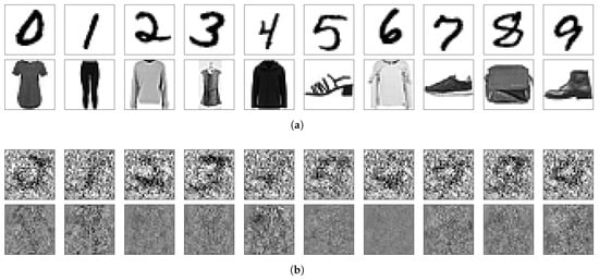
Figure 11.
Comparison of what is visualized by humans and NNs. (a) What we see. (b) What NN sees.

Figure 12.
What another NN sees given the same set of images of digits in the top row of Figure 11a.
5.2. Null Space of NNs and Reliability Issue
Ball [36] pointed out that there are reproducibility and reliability issues with AI. Previously, studies have found that neural network models could pick up on irrelevant features to succeed in classification tasks, raising questions about their reliability. In this paper, the null space analysis on neural networks provides additional insights into these reliability concerns and shows that the NN may pick up on hidden features that are not just irrelevant but that are crafted to confuse the NN. In addition to being too focused on aligning with the particular patterns in the training data, the design of neural network architectures may also raise risks that cannot be solved by merely increasing the data set size. Importantly, it is the architecture that leads to the null space weaknesses shown in this paper.
In addition, stego images created by null space methods cannot be used to improve training. As described in [1], the adversarial example/image is a modified version of a clean image that is intentionally perturbed to mislead machine learning models, such as deep neural networks. Some studies have shown that it may be possible to harden NNs against adversarial attacks. Further, it was observed by Szegedy et al. that the robustness of deep neural networks against adversarial examples could be improved by adversarial training, where the idea is to include adversarial examples in the training data [3]. It is crucial to note that while adversarial examples using previous techniques may improve the training, they cannot solve the problem caused by the null space of a neural network. There are some interesting applications in adversarial attacks [4,37] that might be combined with null space ideas to produce an efficient, reliable way to fool neural networks, and this could be a fruitful direction for future research.
The null space analysis of NNs is not limited to the NNs in image classification tasks. In this study, image steganography is selected as an application to better visualize the impact of the null space. The existence of the null space, inherent in the neural network’s architecture, implies that one can always use the null space vectors to fool a neural network or the user of a neural network, at least when the input data projected onto the null space is close enough to the original to fool a human viewer. Recently, the development of large language models has advanced rapidly. However, these models sometimes produce incorrect or unreasonable outputs. Many researchers have focused on detecting and quantifying the extent of hallucinations in such models [38,39,40]. Through the analysis of the null space of neural networks, the null space may potentially be a contributing cause for these hallucinations. This also suggests a potential future direction for exploring the underlying reasons for hallucinations in large language models.
Author Contributions
Conceptualization, K.M.S.; Methodology, X.L.; Software, X.L.; Validation, K.M.S.; Formal analysis, X.L.; Data curation, X.L.; Writing—original draft, X.L.; Writing—review & editing, K.M.S.; Visualization, X.L.; Supervision, K.M.S.; Project administration, K.M.S. All authors have read and agreed to the published version of the manuscript.
Funding
This research received no external funding.
Data Availability Statement
The code and trained models supporting this study are available from the corresponding author upon request.
Conflicts of Interest
The authors declare that they have no conflicts of interest related to this work.
Appendix A. Pseudocode of the Image Stegonography Method
In this section, the pseudocode of the image stegonography method proposed in Section 3 is provided as follows:
| Algorithm A1 Photo Steganography Method Based on the Null Space of a Neural Network |
|
Appendix B. Proofs and Additional Results from Section 2.1
Appendix B.1. Properties of the Null Space in Nonlinear Maps
Proposition A1.
Let be a nonlinear map. Then the set is a subspace of .
Proof.
First, by definition, , and for every and for every , . Second, when , for every and , we have ; hence . Therefore is a subspace of . □
Proposition A2.
Given a nonlinear map, . For any and , .
Proof.
For any , . □
Given a nonlinear map , as well as its null space , we also considered its null set, . It is easy to see that is a subset of , and may not be a vector space in general. However, also has some structure; any vector in that is not in the subspace is part of a set of integer periodic null elements.
Proposition A3.
Given a nonlinear map , consider the set . If but , then for any integer k, .
Proof.
Let . We prove that and . Indeed, implies that for every ; hence . And implies that for every ; hence . Therefore, if , for any integer k. □
Appendix B.2. Proofs of Lemmas from Section 2.1
Proof of Lemma 1.
Assume the nonlinear map has a decomposition where is linear. For any , holds for every , . Therefore, and is a subspace of with . □
Proof of Lemma 2.
Given the nonlinear map , consider the quotient space , where . The addition , scalar multiplication , and make a vector space (of dimension ). Denote as the quotient map from to (i.e., ). Then, is linear and . Define as the map . To show that is well-defined, notice that when , for some ; hence by the definition of . Now, is the decomposition needed. □
Appendix C. Related Results in Section 2.3
The convolution operation is linear. The convolution of an image and a kernel can also be written in a matrix-vector multiplication form. For example, consider the case of a image convolved with a kernel. Figure A1 and Equation (A1) show the convolution with valid padding and its matrix form. A image convolved with a kernel with valid padding can be written as a matrix (kernel) multiplied with a vector (image).
The convolution with the same padding keeps the input dimension and the output dimension the same by appending zero values in the outer frame of the images. Equation (A2) shows the matrix form of a convolution operation with the same padding; that is, a matrix (kernel) multiplied with a vector.

Figure A1.
Convolution example.
Figure A1.
Convolution example.

We can prove that for almost all cases, the convolution operations with valid padding or the same padding are full rank, i.e., the dimension of the null space is exactly the difference of the dimensions of the input and output. More precisely, consider all the convolution operations convolving inputs with kernels. The set of all kernels can be identified with , and we may equip the Lebesgue measure on the set. The following Lemma shows that, for all but a zero-measure subset of all kernels, the convolution operation has full rank.
Lemma A1.
Let be positive integers and , . For almost all kernels, the (valid padding or same padding) convolution operation of the kernel acting on images has full rank.
Proof.
Let M be the matrix representation of the convolution operation (see Equations (A1) and (A2) for both valid padding and same-padding cases).
To begin with, let us focus on the convolution with valid padding (Equation (A1)). The null space of a convolution operation is . By switching columns in the matrix M, we may assume that there is a weight a of the kernel that appears and only appears on every entry of the diagonal of M. As an example, for the matrix in Equation (A1), we switch the columns with the new order . Then, the diagonal has entries all equal to a. Let be the matrix consisting of the first columns and the first rows of M, which is a square matrix with diagonal entries all equal to a. In the following, we show that has full rank for all but a finite number of choices of a; hence M also has full rank for almost all kernels. We have that is a square matrix and , where I is the identity matrix and B is a square matrix independent of a with diagonal entries all equal to zero. Therefore, is invertible (i.e., has full rank) if and only if is not an eigenvalue of B. Fix the other values in the kernel and only change the value of a; then the matrix B is fixed. While B has many but finite eigenvalues, for every B, for all but a finite number of choices of a, has full rank. Thus, for all but a zero-measure subset of all kernels, and M have full rank.
For the convolution with the same padding, let M be the matrix representation of a given kernel (see Equation (A2)). The diagonal entries are all equal. Following the proof above, we know that M is full rank for almost all kernels. □
Appendix D. Discussion on Parameters in the Null Space-Based Image Steganography Method
This appendix provides theoretical analyses and empirical evidence for the feasible ranges of the parameters used in the construction of the steganographic image
where denotes the orthogonal complements of the hidden image to the model’s null space and denotes the null space projections of the cover image. The design of these parameters is guided by three conditions:
- Every entry of S lies within the normalized range .
- S is classified as the hidden image H by the trained model.
- The visual appearance of S is similar to the cover image C and does not reveal the true digit of H.
Appendix D.1. Condition (1): Range Constraint and Parameter Bounds
Although both the hidden image H and the cover image C are normalized within the range , their components after the null space decomposition,
do not necessarily remain within this range. More specifically, some entries of and may exceed even if the original inputs were normalized.
To ensure that every entry of the stego image lies within , one can fix one parameter and obtain the feasible range of the other parameter accordingly. Without loss of generality, if we first fix the value of , the following must hold to satisfy the range constraint of S:
where is the entry of .
Equation (A3) is a sufficient condition to satisfy the range constraint of S. When this condition is satisfied, it is always possible to choose at least one feasible value of such that each pixel of S is in the range . However, if any entry of already exceeds , there may not exist a value of that can satisfy the range constraint on S. By symmetry, the same applies if is fixed first.
The specific numerical bound for (or ) may vary across data sets. As an illustrative example, we computed the bound of for all training samples in the MNIST data set:
Across the 60,000 training images, the upper bound of has a mean value of 0.7077, with a minimum of 0.4012 and a maximum of 1.0129. Thus, the representative choice used in our experiments with the MNIST data set lies in the safe and numerically valid region for all samples.
Appendix D.2. Condition (2): Classification Consistency
The second condition guarantees the classification consistency of the stego image. More specifically, given a trained neural network f, the stego image should satisfy
However, when becomes too small, the hidden image component may be misclassified and fail to reveal the hidden information. Thus, a sufficiently large is required to ensure a sufficiently large pool of candidate hidden images.
As an illustrative example, we evaluated one trained MNIST network by scaling the training inputs with different values of . The accuracies are shown in Figure A2. In this example, the accuracy remains above 0.95 for , but it drops sharply when . This is consistent with the example provided in Section 4.3, where a very small value for can cause the images to lose contrast, and this loss of contrast contributes to classification with diminished confidence or potential misclassifications. For more complex data sets, a larger may be required.

Figure A2.
Comparison of accuracy with different input scaling ().
Figure A2.
Comparison of accuracy with different input scaling ().

Appendix D.3. Condition (3): Visual Requirements
The third condition considers the visual requirements of the stego image, which also provides an idea to fool the neural network. While the stego image must be correctly recognized by the neural network as the hidden image H, its visual appearance should be similar to the cover image C to the human eye.
The visual similarity between the projected cover component and the original cover image C is determined by the dimension of the network’s null space. A larger null space dimension makes more visually similar to C. The scaling factor controls the contrast level of . A larger makes appear darker and more dominant in the stego image.
For example, Figure A3 shows the stego images with different scaling factors . All stego images are correctly classified by the model as the hidden digit “5” with 100% confidence. However, as increases, decreases, and the projected cover image gradually becomes noisier and less visible.

Figure A3.
Comparison of stego images with different input scaling ().
Figure A3.
Comparison of stego images with different input scaling ().

References
- Akhtar, N.; Mian, A. Threat of Adversarial Attacks on Deep Learning in Computer Vision: A Survey. IEEE Access 2018, 6, 14410–14430. [Google Scholar] [CrossRef]
- Su, J.; Vargas, D.V.; Sakurai, K. One pixel attack for fooling deep neural networks. IEEE Trans. Evol. Comput. 2019, 23, 828–841. [Google Scholar] [CrossRef]
- Szegedy, C.; Zaremba, W.; Sutskever, I.; Bruna, J.; Erhan, D.; Goodfellow, I.J.; Fergus, R. Intriguing properties of neural networks. arXiv 2014, arXiv:1312.6199. [Google Scholar] [CrossRef]
- Goodfellow, I.J.; Shlens, J.; Szegedy, C. Explaining and harnessing adversarial examples. arXiv 2015, arXiv:1412.6572. [Google Scholar] [CrossRef]
- Moosavi-Dezfooli, S.M.; Fawzi, A.; Fawzi, O.; Frossard, P. Universal Adversarial Perturbations. In Proceedings of the IEEE Conference on Computer Vision and Pattern Recognition, Honolulu, HI, USA, 21–26 July 2017; pp. 1765–1773. [Google Scholar]
- Fowl, L.; Goldblum, M.; Chiang, P.y.; Geiping, J.; Czaja, W.; Goldstein, T. Adversarial Examples Make Strong Poisons. In Advances in Neural Information Processing Systems; Ranzato, M., Beygelzimer, A., Dauphin, Y., Liang, P., Vaughan, J.W., Eds.; Curran Associates, Inc.: Red Hook, NY, USA, 2021; Volume 34, pp. 30339–30351. [Google Scholar]
- Ilyas, A.; Santurkar, S.; Tsipras, D.; Engstrom, L.; Tran, B.; Madry, A. Adversarial Examples are Not Bugs, They are Features. In Advances in Neural Information Processing Systems; Wallach, H., Larochelle, H., Beygelzimer, A., d’Alché-Buc, F., Fox, E., Garnett, R., Eds.; Curran Associates, Inc.: Red Hook, NY, USA, 2019; Volume 32. [Google Scholar]
- Cook, M.; Zare, A.; Gader, P. Outlier Detection Through Null Space Analysis of Neural Networks. arXiv 2020, arXiv:2007.01263. [Google Scholar] [CrossRef]
- Rezaei, H.; Sabokrou, M. Quantifying Overfitting: Evaluating Neural Network Performance through Analysis of Null Space. arXiv 2023, arXiv:2305.19424. [Google Scholar] [CrossRef]
- Sonoda, S.; Ishikawa, I.; Ikeda, M. Ghosts in neural networks: Existence, structure and role of infinite-dimensional null space. arXiv 2021, arXiv:2106.04770. [Google Scholar] [CrossRef]
- Schwab, J.; Antholzer, S.; Haltmeier, M. Deep null space learning for inverse problems: Convergence analysis and rates. Inverse Probl. 2019, 35, 025008. [Google Scholar] [CrossRef]
- Kissel, M.; Gottwald, M.; Diepold, K. Neural Network Training with Safe Regularization in the Null Space of Batch Activations. In Artificial Neural Networks and Machine Learning, Proceedings of the ICANN 2020: 29th International Conference on Artificial Neural Networks, Bratislava, Slovakia, 15–18 September 2020; Proceedings, Part II; Springer: Cham, Switzerland, 2020; pp. 217–228. [Google Scholar]
- Wang, S.; Li, X.; Sun, J.; Xu, Z. Training Networks in Null Space of Feature Covariance for Continual Learning. In Proceedings of the IEEE/CVF Conference on Computer Vision and Pattern Recognition, Nashville, TN, USA, 20–25 June 2021; pp. 184–193. [Google Scholar]
- Subramanian, N.; Elharrouss, O.; Al-Maadeed, S.; Bouridane, A. Image steganography: A review of the recent advances. IEEE Access 2021, 9, 23409–23423. [Google Scholar] [CrossRef]
- Hu, K.; Wang, M.; Ma, X.; Chen, J.; Wang, X.; Wang, X. Learning-based image steganography and watermarking: A survey. Expert Syst. Appl. 2024, 249, 123715. [Google Scholar] [CrossRef]
- Hussain, M.; Wahab, A.W.A.; Idris, Y.I.B.; Ho, A.T.; Jung, K.H. Image steganography in spatial domain: A survey. Signal Process. Image Commun. 2018, 65, 46–66. [Google Scholar] [CrossRef]
- Arunkumar, S.; Subramaniyaswamy, V.; Vijayakumar, V.; Chilamkurti, N.; Logesh, R. SVD-based robust image steganographic scheme using RIWT and DCT for secure transmission of medical images. Measurement 2019, 139, 426–437. [Google Scholar] [CrossRef]
- Radeaf, H.S.; Mahmmod, B.M.; Abdulhussain, S.H.; Al-Jumaeily, D. A Steganography Based on Orthogonal Moments. In Proceedings of the International Conference on Information and Communication Technology, Baghdad, Iraq, 15–16 April 2019; pp. 147–153. [Google Scholar]
- Xiao, B.; Luo, J.; Bi, X.; Li, W.; Chen, B. Fractional discrete Tchebyshev moments and their applications in image encryption and watermarking. Inf. Sci. 2020, 516, 545–559. [Google Scholar] [CrossRef]
- Soria-Lorente, A.; Berres, S.; Díaz-Nuñez, Y.; Avila-Domenech, E. Hiding data inside images using orthogonal moments. J. Inf. Secur. Appl. 2022, 67, 103192. [Google Scholar] [CrossRef]
- Yamni, M.; Daoui, A.; Abd El-Latif, A.A. Efficient color image steganography based on new adapted chaotic dynamical system with discrete orthogonal moment transforms. Math. Comput. Simul. 2024, 225, 1170–1198. [Google Scholar] [CrossRef]
- Hassan, G.; Hosny, K.M.; Fathi, I.S. Optimized bio-signal reconstruction and watermarking via enhanced fractional orthogonal moments. Sci. Rep. 2025, 15, 30337. [Google Scholar] [CrossRef] [PubMed]
- Wu, P.; Yang, Y.; Li, X. Image-Into-Image Steganography Using Deep Convolutional Network. In Advances in Multimedia Information Processing, Proceedings of the PCM 2018: 19th Pacific-Rim Conference on Multimedia, Hefei, China, 21–22 September 2018; Proceedings, Part II; Springer: Cham, Switzerland, 2018; pp. 792–802. [Google Scholar]
- Duan, X.; Jia, K.; Li, B.; Guo, D.; Zhang, E.; Qin, C. Reversible image steganography scheme based on a U-Net structure. IEEE Access 2019, 7, 9314–9323. [Google Scholar] [CrossRef]
- Baluja, S. Hiding images within images. IEEE Trans. Pattern Anal. Mach. Intell. 2019, 42, 1685–1697. [Google Scholar] [CrossRef]
- Lu, S.P.; Wang, R.; Zhong, T.; Rosin, P.L. Large-Capacity Image Steganography Based on Invertible Neural Networks. In Proceedings of the IEEE/CVF Conference on Computer Vision and Pattern Recognition, Nashville, TN, USA, 20–25 June 2021; pp. 10816–10825. [Google Scholar]
- Liu, L.; Tang, L.; Zheng, W. Lossless image steganography based on invertible neural networks. Entropy 2022, 24, 1762. [Google Scholar] [CrossRef]
- Shang, F.; Lan, Y.; Yang, J.; Li, E.; Kang, X. Robust data hiding for JPEG images with invertible neural network. Neural Netw. 2023, 163, 219–232. [Google Scholar] [CrossRef]
- Yang, Z.; Wang, Z.; Zhang, X. A general steganographic framework for neural network models. Inf. Sci. 2023, 643, 119250. [Google Scholar] [CrossRef]
- Martín, A.; Hernández, A.; Alazab, M.; Jung, J.; Camacho, D. Evolving Generative Adversarial Networks to improve image steganography. Expert Syst. Appl. 2023, 222, 119841. [Google Scholar] [CrossRef]
- Wang, K.; Zhu, Y.; Chang, Q.; Wang, J.; Yao, Y. High-accuracy image steganography with invertible neural network and generative adversarial network. Signal Process. 2025, 234, 109988. [Google Scholar] [CrossRef]
- LeCun, Y.; Cortes, C.; Burges, C.J. MNIST Handwritten Digit Database; AT&T Labs: Atlanta, GA, USA, 2010. [Google Scholar]
- Xiao, H.; Rasul, K.; Vollgraf, R. Fashion-MNIST: A Novel Image Dataset for Benchmarking Machine Learning Algorithms. arXiv 2017, arXiv:1708.07747. [Google Scholar] [CrossRef]
- Cohen, G.; Afshar, S.; Tapson, J.; Schaik, A.V. EMNIST: Extending MNIST to Handwritten Letters. In Proceedings of the 2017 International Joint Conference on Neural Networks (IJCNN), Anchorage, AK, USA, 14–19 May 2017. [Google Scholar]
- Krizhevsky, A. Learning Multiple Layers of Features from Tiny Images; Technical Report TR-2009; University of Toronto: Toronto, ON, Canada, 2009. [Google Scholar]
- Ball, P. Is AI leading to a reproducibility crisis in science? Nature 2023, 624, 22–25. [Google Scholar] [CrossRef]
- Moosavi-Dezfooli, S.M.; Fawzi, A.; Frossard, P. Deepfool: A Simple and Accurate Method to Fool Deep Neural Networks. In Proceedings of the IEEE Conference on Computer Vision and Pattern Recognition, Las Vegas, NV, USA, 27–30 June 2016; pp. 2574–2582. [Google Scholar]
- Maynez, J.; Narayan, S.; Bohnet, B.; McDonald, R. On faithfulness and factuality in abstractive summarization. arXiv 2020, arXiv:2005.00661. [Google Scholar] [CrossRef]
- Ji, Z.; Lee, N.; Frieske, R.; Yu, T.; Su, D.; Xu, Y.; Ishii, E.; Bang, Y.J.; Madotto, A.; Fung, P. Survey of hallucination in natural language generation. ACM Comput. Surv. 2023, 55, 1–38. [Google Scholar] [CrossRef]
- Jesson, A.; Beltran Velez, N.; Chu, Q.; Karlekar, S.; Kossen, J.; Gal, Y.; Cunningham, J.P.; Blei, D. Estimating the hallucination rate of generative ai. Adv. Neural Inf. Process. Syst. 2024, 37, 31154–31201. [Google Scholar]


Disclaimer/Publisher’s Note: The statements, opinions and data contained in all publications are solely those of the individual author(s) and contributor(s) and not of MDPI and/or the editor(s). MDPI and/or the editor(s) disclaim responsibility for any injury to people or property resulting from any ideas, methods, instructions or products referred to in the content. |
© 2025 by the authors. Licensee MDPI, Basel, Switzerland. This article is an open access article distributed under the terms and conditions of the Creative Commons Attribution (CC BY) license (https://creativecommons.org/licenses/by/4.0/).