Abstract
To address path deviation and efficiency reduction issues in traditional interpolation optimization algorithms for complex path machining, this paper proposes a chord error-priority bilevel interpolation optimization method (CPBI). First, arc length parametric modeling of the machining path is performed within the Frenet–Serret framework, yielding curvature and torsion information. After introducing geometric-based multi-machining constraints in the outer layer, the velocity upper limit is established by controlling chord error to dynamically adjust regions with curvature mutation. In the inner layer, combining the velocity limit with bidirectional scanning achieves adaptive optimization of interpolation step size and optimal velocity planning that balances precision and smoothness. Simulation results demonstrate that CPBI effectively reduces the number of interpolation points by 30–50% while ensuring the chord error. Compared with the reference method, the CPBI improved efficiency by 14.31% and 34.72% in machining experiments on S-shaped and wave-shaped paths, respectively. The results validated the CPBI’s high precision and efficiency advantages in complex path machining, providing an effective solution for CNC path optimization in high-end manufacturing.
Keywords:
chord error; interpolation optimization; path modeling; Frechet-Serret framework; machining efficiency MSC:
68U07
1. Introduction
Path interpolation optimization has important applications in the machining of complex workpieces within high-end manufacturing sectors such as aerospace and precision molds. Since CNC machining achieves material removal by guiding cutting tools along predetermined paths, discontinuities in these paths and velocity irregularities often cause acceleration/deceleration impacts on machine tools, leading to machining errors and surface quality degradation [1,2,3]. To effectively control such issues, it is necessary to achieve path smoothing and rational feed rate allocation through interpolation optimization before machining. Existing research has proposed various interpolation optimization methods. Among them, methods based on polynomials or spline curves can reduce machining errors and optimize feed rates. However, in actual complex path machining, excessive velocity fluctuations or failure to approach the upper limit of permissible velocity often occur, thereby affecting machining efficiency and quality [4,5]. Therefore, it is essential to investigate interpolation optimization methods for complex paths. The objective is to ensure smooth paths and machining accuracy while enhancing the machine tool’s velocity utilization and overall machining efficiency.
Existing research on machining path interpolation optimization primarily focuses on curve parameterization and CNC constraint models, forming two main lines of inquiry centered on path interpolation and feed rate optimization [6,7,8].
The research on machining path interpolation has primarily focused on improving interpolation algorithms to enhance path accuracy, smoothness, and machining efficiency [8,9]. To overcome the issues of velocity discontinuity and acceleration mutation caused by traditional linear interpolation, parametric curve interpolation (such as NURBS and B-spline curves) has become the mainstream research approach [10]. Jia et al. proposed an adaptive NURBS curve interpolation algorithm that effectively reduces contour errors by dynamically adjusting the feed rate in real time to accommodate curvature variations [11]. Wang et al. deeply integrated feed rate scheduling with the interpolation process, considering machine tool dynamic constraints before generating interpolation points to achieve high-precision predictive interpolation [12]. Song et al. focused on the smooth connection of short-segment paths, employing B-spline curves to smooth discrete paths, significantly reducing machine tool vibration during machining [13]. However, most of the above studies focus on macro-path interpolation, while challenges remain in achieving smoothness and velocity planning at corners for high-precision machining paths. To address this issue, some scholars have proposed intelligent interpolation methods to enhance interpolation performance under complex paths. Sun et al. developed a neural network-based interpolation points prediction model that rapidly generates smooth interpolation sequences meeting accuracy requirements by learning optimal machining data [14]. Ward proposed a data-driven framework for adaptive adjustment of interpolation parameters to address uncertainties in the machining process [15]. Although these intelligent methods demonstrate significant potential in specific scenarios, they suffer from issues such as high dependence on training data and poor reliability when deployed in actual CNC systems.
The research on feed rate optimization focuses on generating continuous velocity curves that satisfy machine tool physical constraints, thereby reducing machining time while ensuring processing quality [16,17]. S-curve velocity planning technology serves as the foundational research in this field [18]. Sencer et al. effectively addressed the corner velocity issue by smoothly connecting multi-segment S-curves while considering trajectory contour error constraints [19]. Sun et al. effectively reduced velocity fluctuations in regions of curvature change by introducing adaptive NURBS interpolation with curvature and driving constraints [20]. Sang et al. optimized the feed rate by establishing a linear relationship between geometric error and feed rate, combined with kinematic constraints [21]. Xu et al. optimized machining paths by proposing a dual NURBS interpolation technique for primary and secondary surfaces, thereby enhancing machining stability and precision [2]. Liu et al. employed arc length compensation and iterative methods to reduce step error and feed rate fluctuations [22]. Although the above studies mostly employ curvature and kinematic parameters as constraint objectives, they provide insufficient support for step-size adaptation and global error consistency on paths with frequent curvature changes at multiple locations. In recent years, scholars have begun exploring feed rate optimization methods based on optimization theory to achieve optimal quality or efficiency. Zhao et al. modeled the feed rate optimization problem as a constrained optimization problem and solved it using the pseudo-spectral method, obtaining the optimal feed rate curve [23]. Yang et al. proposed a feed rate optimization method based on the PSO to balance machining time and accuracy, achieving multi-objective optimization [17]. Wang et al. introduced model prediction methods for feed rate optimization, enhancing the robustness of feed rate scheduling by compensating for model errors through rolling optimization [24]. Although these optimization methods can achieve superior performance, their substantial computational demands limit their applicability, making them primarily used for interpolation optimization in simplified models. Balancing optimality and applicability remains a key challenge in this field.
To address these issues, this paper proposes a chord error-priority bilevel interpolation optimization method, offering a novel solution for achieving high-precision and high-efficiency interpolation in complex machining paths. The method’s advantage lies in its geometry-driven path modeling and the introduction of multiple kinematic constraints. Utilizing the Frenet–Serret framework to extract curve information ensures path continuity and preservation of geometric properties. Simultaneously, the concept of bilevel interpolation optimization was introduced, which not only ensures minimal chord error but also achieves adaptive optimization of interpolation step size and feed rate through a bidirectional scanning method.
2. Machining Path Modeling
2.1. Arc Length Parameterization of Path
In practical machining, complex paths are typically composed of multiple segments of curves with fast curvature changes. This paper uses non-uniform B-spline curves as an example for path modeling. First, the curve construction is defined according to Equation (1).
where denotes the control points of the curve, totaling points. represents the curve’s basis functions, with being the degree of the basis function. It also indicates the repetition degree of the curve generated by the control points at the start and end positions. The basis functions of a B-spline curve are th-degree piecewise polynomials determined by the knot vectors , where the parameters satisfy . The recursive equation for a B-spline curve is as follows.
Then the derivative of the curve with respect to u can be inferred from the derivative of the basis function:
The explicit expression for the derivative of a first-order basis function is as follows:
Terms with a denominator of zero are treated as zero. Higher-order derivatives of basis functions can be derived recursively as follows:
The advantage of using arc length as the parameter is that it is independent of the feed rate along the curve and is also unaffected by the choice of coordinate system. The arc length parameterization of the machining curve obtains the arc length function as shown in Equation (8). Subsequently, the tangential velocity is calculated as shown in Equation (9).
The value of is obtained through Gaussian integration and combined with Newton’s iteration method to invert for , as shown in Equation (10) [25]. Finally, the arc length parameter curve can be calculated as in Equation (11):
2.2. Path Curve Expansion Based on the Frenet–Serret Framework
The Frenet–Serret framework is a coordinate system method for automatic path planning. It describes the local geometry of a path curve using two scalar quantities (curvature and torsion) and provides an orthogonal, concise, and intuitionistic local coordinate system. This paper adopts this framework to further expand the machining path, which is structured as follows:
where , , and represent the tangent, principal normal, and secondary normal vector, respectively. denotes curvature, and denotes torsion. Combining the above formulas, the curvature and torsion of the curve are expressed as follows:
Then the arc length derivative is obtained as in Equation (19).
The value of can be obtained by the difference between equal-arc-length meshes of the curve.
The machining path and arc-length path obtained from Section 2.1 have a fixed interpolation period of Let the arc length velocity be , and the single-step arc length be . The chord error represents the maximum deviation of the chord connecting the two machining interpolation points from the intended motion path, as shown in Figure 1. It can be seen that during actual machining, the tool’s interpolation path moves in a straight line along the machining point, resulting in the actual path failing to coincide with the desired path. Moreover, this phenomenon becomes more pronounced in areas of greater curvature, leading to larger velocity fluctuations and potentially causing single-axis acceleration to exceed limits. Therefore, it is necessary to control the chord error to avoid this situation as much as possible, thereby ensuring machining smoothness and improving machining quality. The equation for chord error is as follows.
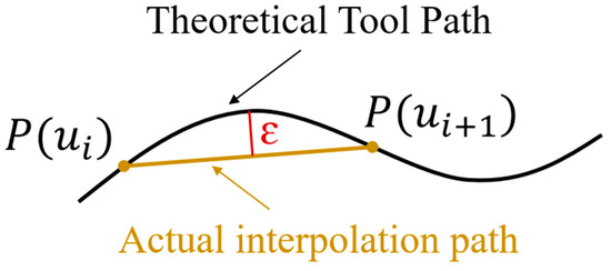
Figure 1.
Chord difference and parameter curve points.
Perform a Taylor expansion at based on the Frenet–Serret framework.
The expression for the chord error can be derived from Equations (20) and (21). For the specific derivation process, refer to Appendix A. The triangle inequality can be used to derive the chord error constraint.
where represents the maximum target chord error. This ensures reasonable optimization of the machining step size under the constraint of maximum chord error. Let and . This yields the current step size constraint, which is dense in areas of high curvature and sparse in areas of low curvature.
2.3. Geometry-Driven Machining Constraints
In actual machining operations, the feed rate of machine tools is often subject to an upper limit. Assuming the feed rate is , common constraints include the following points:
Comprehensive velocity constraints for each axis:
Tangential acceleration constraint:
Normal acceleration constraint:
Jerk Constraint:
where denotes the first derivatives of velocity with respect to arc length. denotes the first derivative of curvature with respect to arc length. For the specific derivation process, refer to Appendix B. From the above five constraints, the point-state velocity upper limit of the machining tools is derived as follows.
where is the upper limit of velocity, and are the upper limits of tangential and normal acceleration, respectively, and is the upper limit of jerk acceleration.
3. A Chord Error-Priority Bilevel Interpolation Optimization Method
3.1. Outer Layer—Global Velocity Optimization of Chord Error-Priority
From the single-step arc length, it follows that at each position s, the following inequality for feed rate is present.
Taking the maximum positive real root of this cubic polynomial as the velocity upper limit dominated by the chord error, then Equation (30) can be obtained.
If , then is minimal, yielding the quadratic solution ; if , then is minimal, yielding the cubic solution .
3.2. Inner Layer—Interpolation Optimization Under Comprehensive Constraints
The comprehensive upper limit for feed rates can be derived from the machine tool point-state velocity limit defined by Equation (28).
Tangential acceleration can be expressed as , and in the arc length domain it can be represented as follows.
To avoid feed rate interpolation distortion caused by excessive step size, further constraints on the step size are required, as shown in Equation (33).
where represents the step velocity variation parameter for adjacent tool positions, with . Combining Equations (23) and (33) yields the final optimized step size as shown in Equation (34).
Based on the optimal step size, the forward and backward scanning equation for the interpolation point obtained from Equation (34) is given by Equations (35) and (36).
where Equation (35) represents forward scanning, while Equation (36) represents backward scanning. denotes the -th discrete arc length parameter, . represents the number of interpolation points. is the fixed interpolation period. The initial point location for bidirectional scanning is selected as the starting point of the machining path. The initial value of the scanning iteration is set as the comprehensive upper limit of the velocity. The iteration termination condition is based on a fixed scanning count , where . The value of is determined according to the complexity of the path. The bidirectional scanning proceeds until iteration ceases to update, ultimately yielding the maximum feasible interpolation point that satisfies multiple constraints and the upper limit of chord error.
According to the scanning equations, a higher average velocity corresponds to a larger arc length per step. Consequently, a shorter number of interpolation points is required for a given machining path. During forward scanning only, the kinematic constraints of subsequent points remain unknown, resulting in conservative velocity estimates for interpolated points. However, backward scanning acquires information from the forward scanning pass. Since the constraints are now known, the velocity of interpolated points can be adjusted to approach the upper limit more closely. Therefore, employing the bidirectional scanning can effectively reduce the number of interpolated points required.
Let , then the actual machining time can be expressed by Equation (38).
where denotes the total arc length of the machining path; represents the optimal velocity solution; is the smallest positive number to prevent the denominator from being 0. For a given , Equation (38) yields the shortest-time discrete solution under the constraints of Equations (33)–(37).
Based on the parametric method for tool paths and the analysis of interpolation optimization for inner and outer layers, the method flowchart for the chord error-priority bilevel interpolation optimization method is shown in Figure 2. Based on Figure 2, the specific implementation steps of this method are as follows:
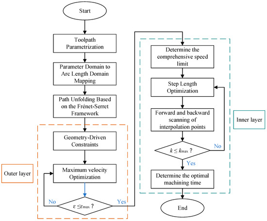
Figure 2.
Flowchart of the chord error-priority bilevel interpolation optimization method.
- Step 1: Initialize kinematic upper limits based on machine tool parameters.
- Step 2: Parametric machining paths based on the Frenet–Serret framework.
- Step 3: Calculate and set multi-kinematic constraints driven by geometry.
- Step 4: By determining the constraints of chordal error, the maximum feed rate is then calculated.
- Step 5: Based on comprehensive constraints, the feed rate and optimal step length are calculated using forward and backward scanning methods to determine the interpolation points.
4. Simulation Verification and Comparison
4.1. Machining Simulation Experiment for S-Shaped Path
To validate the performance of the proposed chord error-priority bilevel interpolation optimization method, this paper first selects an S-shaped machining path for simulation experiments. The S-shaped machining path is achieved by constructing a quasi-uniform rational B-spline curve of order 3, i.e., . The endpoints have order , while the intermediate nodes are approximated as equidistant. There are control points , , , …, . The basis functions for the i-th segment are given by Equation (39).
Based on the parameters in the above equation, the specific form of each segment can be expressed as Equation (39). The final processed path obtained is an S-shaped quasi-uniform rational curve, as shown in Figure 3. In this case, the number of control points is 16, and the node vector is . The program for generating machining paths can be found in the Supplementary Materials documents.
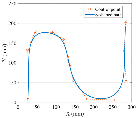
Figure 3.
S-shaped machining path and control points.
Based on the characteristics of the S-shaped machining path, it is necessary to understand how the machining path varies with changes in the parameter domain, as shown in Figure 4. Simultaneously, the velocity of the path curve relative to parameter u is represented as shown in Figure 5. Further conversion of the parameter domain of this machining path into the arc length domain is shown in Figure 6. It can be observed that the arc length is unequal in steps in the parameter domain, which further highlights the necessity of velocity limiting in the arc length domain.
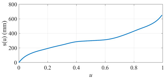
Figure 4.
Parameter domain function of the path.
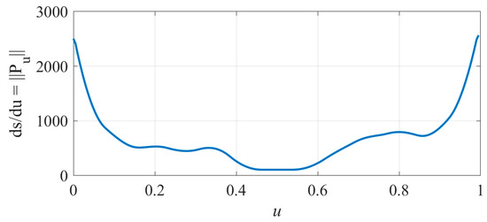
Figure 5.
The rate of change in arc length with respect to the parameter u.
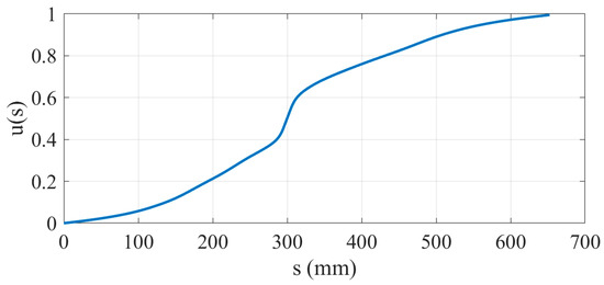
Figure 6.
Mapping from the parameter domain to the arc length domain.
Since this paper expands the machining path based on the Frenet–Serret framework, curvature information is indispensable. The curvature visualization of the S-shaped machining path is shown in Figure 7. It can be observed that the curve exhibits abrupt curvature changes at certain positions, which easily restrict the feed rate and impact machining efficiency. Therefore, performing interpolation optimization at these positions can effectively achieve smooth transitions in the machining path.
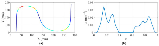
Figure 7.
Curvature analysis of machining paths: (a) attachment of path curvature (color indicates the magnitude of curvature); (b) curve of path curvature.
Based on path characteristics and machining requirements, it is necessary to set up complete simulation constraints. These include geometric parameters of the machining path, interpolation cycles, and multiple kinematic constraints. Specific experimental parameters are shown in Table 1.

Table 1.
Experimental parameters for S-shaped machining path.
Combining the experimental parameters from Table 1, the proposed method CPBI was applied to optimize the S-shaped path through simulation. The resulting path interpolation is shown in Figure 8. As shown in Figure 8, the initial number of interpolation points for the machining path is 200. After interpolation optimization, the number of interpolation points is reduced to 128, indicating that CPBI can effectively improve the computational efficiency of toolpath points. If only forward or backward scanning methods are used for interpolation optimization, the number of interpolation points will increase to 177. Meanwhile, the chord error after interpolation optimization is shown in Figure 9. Meanwhile, the chord error after interpolation optimization is shown in Figure 9. It can be seen that the chord error is controlled within 0.0002 mm, far below the specified upper limit for chord error . This indicates that the error when machining along this interpolation-optimized path is extremely minimal. Note that the velocity variation parameter is introduced in Section 3.2. The selection of this value affects both the number of interpolation points and the chord error, as detailed in Table 2. As shown in Table 2, when , the number of interpolation points is 184, with a maximum chord error of 0.0001 mm; When , the number of interpolation points is 97, with a maximum chord error of 0.0006 mm; when , a balance between the number of interpolation points and the maximum chord error is achieved. At the same time, an excessively large is more likely to cause abrupt velocity changes. To ensure the algorithm’s optimality, η = 0.15 is selected for the simulations in this paper.
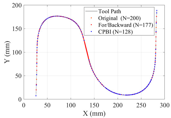
Figure 8.
Position of machining points before and after interpolation optimization for the S-shaped path.
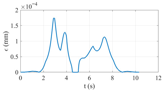
Figure 9.
Chord error curve of S-shaped path.
Table 2.
Sensitivity analysis of velocity variation parameters .
To validate the superiority of the proposed CPBI method, the iteration control vector parametrization method (ICVP) [26] was selected as a comparison. Simulations comparing the feed rates of both methods are shown in Figure 10. As shown in Figure 10, the ICVP maintains feed rates within the permissible range throughout the process. However, at locations with fast curvature changes, it adopts a constant-velocity machining strategy approaching the minimum feed rate. Therefore, this method can accomplish high-precision machining for S-shaped path but it inevitably increases machining time. In comparison, the feed rate curve obtained by CPBI not only avoids exceeding the limit but also better fits the permissible feed rate curve in regions with fast curvature changes. Furthermore, in the S-shaped machining path experiment, the CPBI algorithm achieved a 14.31% improvement in machining efficiency compared to the ICVP. Based on a comprehensive analysis of the results in Figure 9 and Figure 10, it can be concluded that the proposed CPBI method can achieve high-precision and high-efficiency machining for an S-shaped path while satisfying multiple machining constraints.
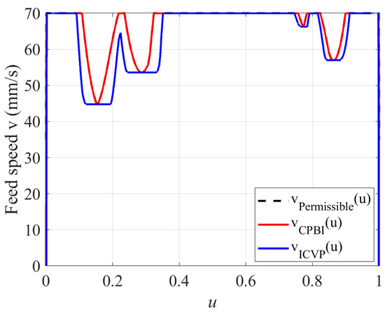
Figure 10.
Comparison of feed rates before and after interpolation optimization for the S-shaped path.
Due to the constraints imposed by acceleration and jerk limits during actual machining processes, it is necessary to conduct further analysis of tangential acceleration, normal acceleration, and jerk accelerated acceleration. The results are shown in Figure 11. As evident from Figure 11, all three parameters remain within the maximum permissible ranges specified in Table 1. Then it can be further demonstrated that the CBPI method is effective for interpolation optimization of the S-shaped machining path.
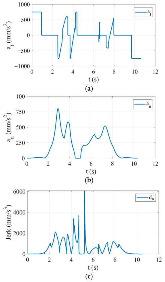
Figure 11.
Relevant machining parameters for S-shaped path velocity planning (a) Tangential acceleration (b) Normal acceleration (c) Jerk accelerated acceleration.
4.2. Machining Simulation Experiment for Wave-Shaped Path
To further validate the effectiveness of CBPI for machining paths featuring multiple high-curvature segments and fast curvature changes, this paper additionally designed a wavy-shaped machining path as the experimental simulation object [5]. This machining path is achieved by constructing a non-uniform rational B-spline curve, where = 3. There are 20 control points: , , , …, . The general weight is . High-curvature regions are constructed with larger weights: and . The uniformly distributed node vectors are . Combining with Equation (2), the wave-shaped path can be expressed as follows:
Based on Equation (40), the designed path curve is shown in Figure 12. As seen in Figure 12, this machining path exhibits both high curvature and fast curvature variations. Upon further calculation, the curvature curve of the wave-shaped machining path is shown in Figure 13. It can be seen that there are over 10 locations with abrupt changes in curve curvature, which makes feed rate optimization more challenging. The program for generating machining paths can be found in the Supplementary Materials documents. Therefore, the proposed CBPI method is applied to perform interpolation optimization for this machining path, thereby demonstrating the high adaptability of the method.
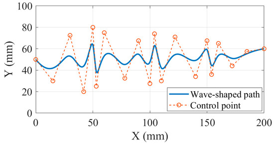
Figure 12.
Wave-shaped machining path and control points.
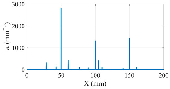
Figure 13.
Curvature curve of the wave-shaped path.
Based on path characteristics and machining requirements, the simulation parameters for the wavy path are set, including the geometric parameters of the path, the interpolation cycle, and multiple kinematic constraints. Specific parameters are shown in Table 3.
Table 3.
Experimental parameters for wave-shaped machining path.
According to Table 3, the CPBI algorithm was employed to optimize the wave-shaped machining path. The interpolation optimization results are shown in Figure 14. The results indicate that the initial number of interpolation points for the wave-shaped machining path was 300, which was reduced to 151 after interpolation optimization. The reduction ratio approached 50%, significantly decreasing the number of machining instructions and enhancing machining efficiency. Similarly, if only forward or backward scanning methods are used for interpolation optimization, the number of interpolation points would increase to 238. Meanwhile, the chord error after interpolation optimization is shown in Figure 15. The optimization method effectively controls it within 0.00035 mm, far below the upper limit of chord error . Further comparisons were conducted using the CPBI method and ICVP method to evaluate the computational time, number of interpolation points, and maximum chord error for wave-shaped path optimization, as detailed in Table 4. As shown in Table 4, the CPBI method demonstrates improvements over the ICVP method in both computational time and the number of interpolation points, while exhibiting essentially identical maximum chord errors. This demonstrates that the CPBI method can reliably ensure the machining accuracy requirements for wave-shaped paths.
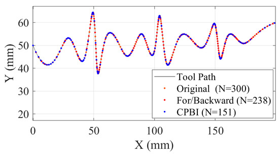
Figure 14.
Position of machining points before and after interpolation optimization for wave-shaped path.
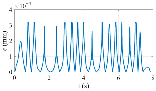
Figure 15.
Chord error curve of wave-shaped path.
Table 4.
Optimization comparison of CPBI and ICVP methods for wave-shaped paths.
Similarly, comparing the feed rate optimized by the CPBI method with that of the ICVP, the results are shown in Figure 16. As shown, the optimized feed rates from both methods remain within the permissible feed rate. However, the feed rate curve optimized by the CPBI method is significantly closer to the permissible feed rate compared to the ICVP. In contrast, in the wave-shaped machining path experiment, the CBPI algorithm improves machining efficiency by 34.72% compared to the ICVP while satisfying multiple machining constraints. Combined analysis of Figure 15 and Figure 16 further demonstrates that the CBPI algorithm is equally applicable to interpolation optimization for machining paths characterized by high curvature and fast curvature changes. It can effectively achieve high-precision and high-efficiency machining of wave-shaped paths.
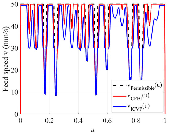
Figure 16.
Comparison of feed rates before and after interpolation optimization for wave-shaped path.
After interpolation optimization of the wave-shaped path using the CBPI method, the resulting tangential acceleration, normal acceleration, and jerk accelerated acceleration are shown in Figure 17. As shown in the figure, all three parameters fall within the maximum permissible ranges specified in Table 3. In summary, the CBPI method proposed in this paper can generate optimized toolpaths with high precision under complex path machining conditions while significantly improving machining efficiency.
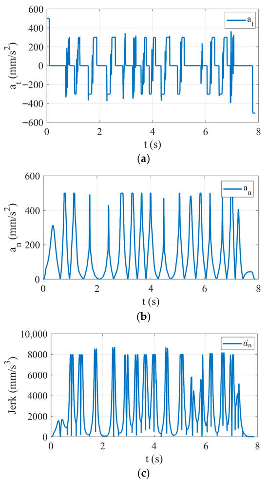
Figure 17.
Relevant machining parameters for wave-shaped path velocity planning: (a) tangential acceleration; (b) normal acceleration; (c) jerk-accelerated acceleration.
5. Conclusions
This paper proposes a chord error-priority bilevel interpolation optimization method for complex path planning. Through global velocity optimization of chord error priority in the outer layer and interpolation optimization under comprehensive constraints in the inner layer, high-precision and high-efficiency machining is achieved for complex curvature paths. Experimental results demonstrate that the CPBI method effectively controls chord error while maintaining machining accuracy. It also significantly reduces the number of interpolation points and increases feed rate while ensuring tangential acceleration, normal acceleration, and jerk accelerated acceleration remain within permissible ranges. Compared to the ICVP, CPBI can improve machining efficiency by 14.31% and 34.72% on S-shaped and wave-shaped paths, respectively. This demonstrates its excellent adaptability and broad application prospects in the interpolation optimization of complex machining paths.
Future work will first demonstrate the effectiveness of the CPBI method in practical machining applications. By addressing potential issues encountered in machining experiments and multi-axis environments (e.g., the impact of tool wear or machine tool rigidity), further expand and improve the CPBI method. Concurrently, deep learning and AI technologies represent key directions for future development. It is essential to explore methods integrating interpolation optimization with these technologies. This will significantly promote its engineering applications in high-precision machining of complex parts.
Supplementary Materials
The following supporting information can be downloaded at: https://www.mdpi.com/article/10.3390/math13213385/s1, Document S1: the basic information for S-shaped machining path; Document S2: the basic information for wave-shaped machining path.
Author Contributions
Conceptualization, P.W., X.Y. and J.Q.; methodology, software, investigation, resources, visualization, writing—original draft preparation, P.W.; validation, L.W., X.Y. and J.Q.; data curation, X.Y. and D.W.; writing—review and editing, P.W. and J.Q.; project administration, L.W., X.Y. and D.W.; funding acquisition, L.W. and J.Q. All authors have read and agreed to the published version of the manuscript.
Funding
This research was supported by the National Natural Science Foundation of China (Nos. 52375448, 52305480).
Data Availability Statement
The original contributions presented in this study are included in the Supplementary Material. Further inquiries can be directed to the corresponding author.
Conflicts of Interest
The authors confirm that the research was conducted in the absence of any commercial or financial relationships that could be construed as a potential conflict of interest.
Abbreviations
The following abbreviations are used in this manuscript:
| CPBI | Chord error- priority bilevel interpolation optimization method |
| CNC | Computer numerical control |
| NURBS | Non-uniform rational B-spline |
| ICVP | Iteration control vector parametrization |
Appendix A
Derivation Process of Chord Error Inequality (Equation (22))
Combining Equations (12)–(18) in the main paper, the following equations can be further derived within the Frenet–Serret framework:
The first, second, and third derivatives are as follows:
Performing a third-order Taylor expansion of curve at , Equation (21) in the main paper is obtained. Then the chord vector can be expressed as follows:
The components of the chord vector in can be expressed as follows:
The third-order approximation of the chord length can be expressed as follows:
Further, the unit chord vector can be obtained.
Correspondingly, the components of vector in can be expressed as follows:
The vector from the start point to the midpoint of the chord is represented as follows:
Correspondingly, the components of vector in can be expressed as follows:
The chord error is defined as the difference between two adjacent machining points and the theoretical circular arc path. Then its expression can be represented as the vector m and the orthogonal distance to the line of the adjacent point.
where
Then the chord error vector can be expressed as follows:
Substituting the Equations (A13), (A14) and (A20) into Equation (A21) yields the following:
By combining the above various equations, the chord error vector for the third-order Taylor expansion can be obtained.
Then the modulus of the chord error is as follows:
From this, Equation (22) in the main paper can be derived.
Appendix B
Jerk is the derivative of normal acceleration with respect to time. It is expressed as follows:
where , and are the normal vector, binormal vector, and tangent vector, respectively.
The two sub-terms in Equation (A26) are calculated as follows:
where denotes the first derivatives of feed rate with respect to arc length. denotes the first derivative of curvature with respect to arc length.
Substituting Equations (A27) and (A28) into Equation (A26) yields the complete jerk equation.
As seen in Equation (27) in the main paper, the tangential component has been omitted. This is because, for ensuring surface quality in actual feed operations, the focus lies on variations in normal acceleration. Since the tangential component does not contribute to normal jerk, it has been omitted. Consequently, Equation (27) in the main paper is derived.
Appendix C
Table A1.
Unified list of symbols.
Table A1.
Unified list of symbols.
| Symbols | Meaning of the Symbol |
|---|---|
| Parametric curve equation | |
| Control point | |
| Basis function | |
| First derivative of the parameter curve with respect to u | |
| Second derivative of the parameter curve with respect to u | |
| Third derivative of the parameter curve with respect to u | |
| Arc length curve equation | |
| Tangent vector | |
| Principal normal vector | |
| Secondary normal vector | |
| Curvature | |
| Torsion | |
| The first derivative of curvature with respect to arc length | |
| The -th discrete arc length parameter | |
| The -th step velocity | |
| Single-step arc length | |
| Maximum Iterations for Bidirectional Scanning | |
| Chord error | |
| The maximum target chord error | |
| velocity | |
| The upper limit of velocity | |
| Tangential acceleration | |
| The upper limits of tangential acceleration | |
| Normal acceleration | |
| The upper limits of normal acceleration | |
| Jerk acceleration | |
| The first derivatives of velocity with respect to arc length | |
| the point-state velocity upper limit of the machining tools | |
| The upper limit of jerk acceleration | |
| The upper limit of velocity dominated by the chord error | |
| The comprehensive upper limit for velocity | |
| The step velocity variation parameter for adjacent tool positions | |
| Single-step arc length under distortion constraints | |
| Single-step arc length under chord error constraints | |
| Interpolation period | |
| Actual machining time | |
| The optimal velocity solution | |
| The smallest positive number to prevent the denominator from being 0 | |
| The total arc length of machining path | |
| Tangent component of the parameter curve | |
| Principal normal component of the parameter curve | |
| Secondary normal component of the parameter curve | |
| The vector from the start point to the midpoint of the chord | |
| Tangent component of | |
| Principal normal component of | |
| Secondary normal component of | |
| chord error vector |
References
- Hu, Y.; Jin, X.; Jiang, X.; Zheng, Z. Inverse kinematics model and trajectory generation of a dual-stage micro milling machine. J. Manuf. Process. 2024, 132, 425–450. [Google Scholar] [CrossRef]
- Xu, Y.; Zaman, M.; Zhou, F. Optimized dual NURBS curve interpolation for high-accuracy five-axis CNC path planning. Sci. Rep. 2025, 15, 25409. [Google Scholar] [CrossRef] [PubMed]
- Lu, Z.; Yang, X.; Zhao, J. Tool-path planning method for kinematics optimization of blade machining on five-axis machine tool. Int. J. Adv. Manuf. Technol. 2022, 121, 1253–1267. [Google Scholar] [CrossRef]
- Liao, Z.; Li, J.; Xie, H.; Wang, Q.; Zhou, X. Region-based toolpath generation for robotic milling of freeform surfaces with stiffness optimization. Robot. Comput. Integr. Manuf. 2020, 64, 101953. [Google Scholar] [CrossRef]
- Wang, L.; Zhang, J.; Li, W.; Wang, Y.; Zhou, Y. Research on feedrate scheduling method for NURBS toolpath interpolation in high-speed CNC machining. Int. J. Adv. Manuf. Technol. 2025, 138, 3293–3313. [Google Scholar] [CrossRef]
- Zhong, W.; Luo, X.; Chang, W.; Cai, Y.; Ding, F.; Liu, H.; Sun, Y. Toolpath Interpolation and Smoothing for Computer Numerical Control Machining of Freeform Surfaces: A Review. Int. J. Autom. Comput. 2019, 17, 1–16. [Google Scholar] [CrossRef]
- Ma, H.; Shen, L.; Jiang, X.; Zou, Q.; Yuan, C. A survey of path planning and feedrate interpolation in computer numerical control. J. Graph. 2022, 43, 967–986. [Google Scholar] [CrossRef]
- Zhou, Y.; Jiang, Y.; Lu, C.; Huang, J.; Pei, J. A review of 5-axis milling techniques for centrifugal impellers: Tool-path generation and deformation control. J. Manuf. Process. 2024, 132, 160–186. [Google Scholar] [CrossRef]
- Zhou, X. An Adapted NURBS Interpolator with a Switched Optimized Method of Feed-Rate Scheduling. Machines 2024, 12, 186. [Google Scholar] [CrossRef]
- Zhang, G.; Gao, J.; Zhang, L.; Wang, X.; Luo, Y. Generalised NURBS interpolator with nonlinear feedrate scheduling and interpolation error compensation. Int. J. Mach. Tools Manuf. 2022, 183, 103956. [Google Scholar] [CrossRef]
- Jia, Z.; Song, D.; Ma, J.; Hu, G.; Su, W. A NURBS interpolator with constant speed at feedrate-sensitive regions under drive and contour-error constraints. Int. J. Mach. Tools Manuf. 2017, 116, 1–17. [Google Scholar] [CrossRef]
- Wang, L.; Liu, Q.; Sun, P.; Lv, S.; Yang, R.; Yang, Z. Dynamic look-ahead feedrate scheduling method based on sliding mode velocity control. Sci. Rep. 2024, 14, 15424. [Google Scholar] [CrossRef]
- Song, D.; Ma, J.; Zhong, Y.; Yao, J. Global smoothing of short line segment toolpaths by control-point-assigning-based geometric smoothing and FIR filtering-based motion smoothing. Mech. Syst. Signal Process. 2021, 160, 107908. [Google Scholar] [CrossRef]
- Sun, C.; Dominguez-Caballero, J.; Ward, R.; Ayvar-Soberanis, S.; Curtis, D. Machining cycle time prediction: Data-driven modelling of machine tool feedrate behavior with neural networks. Robot. Comput. Integr. Manuf. 2022, 75, 102293. [Google Scholar] [CrossRef]
- Ward, R.; Sun, C.; Dominguez-Caballero, J.; Ojo, S.; Ayvar-Soberanis, S.; Curtis, D.; Ozturk, E. Machining Digital Twin using real-time model-based simulations and lookahead function for closed loop machining control. Int. J. Adv. Manuf. Technol. 2021, 117, 3615–3629. [Google Scholar] [CrossRef]
- Sun, S.; Zhao, P.; Zhang, T.; Li, B.; Yu, D. Smoothing interpolation of five-axis tool path with less feedrate fluctuation and higher computation efficiency. J. Manuf. Process. 2024, 109, 669–693. [Google Scholar] [CrossRef]
- Yang, J.; Yin, X.; Sun, Y. PSO-Based Feedrate Optimization Algorithm for Five-Axis Machining with Constraint of Contour Error. Machines 2023, 11, 501. [Google Scholar] [CrossRef]
- Wang, Y.; Xie, Z.; Xie, F.; Liu, X. A symmetrical arrangement strategy based real-time toolpath planning method for a 5-DoF fully parallel machining robot. Int. J. Adv. Manuf. Technol. 2024, 134, 2299–2317. [Google Scholar] [CrossRef]
- Sencer, B.; Ishizaki, K.; Shamoto, E. High speed cornering strategy with confined contour error and vibration suppression for CNC machine tools. CIRP Ann. Manuf. Technol. 2015, 64, 369–372. [Google Scholar] [CrossRef]
- Sun, Y.; Zhao, Y.; Bao, Y.; Guo, D. A novel adaptive feedrate interpolation method for NURBS tool path with drive constraints. Int. J. Mach. Tools Manuf. 2014, 77, 74–81. [Google Scholar] [CrossRef]
- Sang, Y.; Yao, C.; Lv, Y.; He, G. An improved feedrate scheduling method for NURBS interpolation in five-axis machining. Precis. Eng. 2020, 64, 70–90. [Google Scholar] [CrossRef]
- Liu, X.; Yu, P.; Chen, H.; Peng, B.; Wang, Z.; Liang, F. Feedrate fluctuation minimization for NURBS tool path interpolation based on arc length compensation and iteration. Micromachines 2025, 16, 402. [Google Scholar] [CrossRef]
- Zhao, K.; Kang, Z.; Guo, X. Smooth Trajectory Generation for Predefined Path with Pseudo Spectral Method. IEEE Access 2020, 8, 158735–158744. [Google Scholar] [CrossRef]
- Wang, L.; Yang, R.; Lv, S.; Yang, Z.; Xin, S.; Liu, Y.; Liu, Q. Combined contour error control method for five-axis machine tools based on digital twin. Sci. Rep. 2025, 15, 17809. [Google Scholar] [CrossRef] [PubMed]
- Wang, J.; Song, C.; Zhang, D.; Li, D.; Qu, S. Fast and Stable Iterative Algorithm for Searching Wheel-Rail Contact Point Based on Geometry Constraint Equations. J. Comput. Nonlinear Dyn. 2023, 18, 011004. [Google Scholar] [CrossRef]
- Ma, H.; Yuan, C.; Shen, L.; Gao, X. Optimal feedrate planning on a five-axis parametric tool path with global geometric and kinematic constraints. J. Comput. Des. Eng. 2022, 9, 2355–2374. [Google Scholar] [CrossRef]


Disclaimer/Publisher’s Note: The statements, opinions and data contained in all publications are solely those of the individual author(s) and contributor(s) and not of MDPI and/or the editor(s). MDPI and/or the editor(s) disclaim responsibility for any injury to people or property resulting from any ideas, methods, instructions or products referred to in the content. |
© 2025 by the authors. Licensee MDPI, Basel, Switzerland. This article is an open access article distributed under the terms and conditions of the Creative Commons Attribution (CC BY) license (https://creativecommons.org/licenses/by/4.0/).