Abstract
The control of infectious diseases plays a critical role in safeguarding the health of species and ecosystems. In this study, we investigate the combined effects of prey refuge and harvesting as mechanisms to limit the spread of disease within predator populations. A deterministic model is developed to examine the system dynamics through local stability analysis of equilibria, and the framework is further extended to an uncertain setting via a fuzzified model. The analysis shows that for small refuge values, the system reaches a stable state where infected predators move toward extinction, while prey and susceptible predators exhibit strong oscillations. As the refuge increases, the system undergoes a Hopf bifurcation, transitioning from periodic oscillations to a stable interior equilibrium. Beyond a critical threshold, oscillations disappear entirely. Harvesting of susceptible predators reveals that moderate harvesting induces oscillatory behavior in both prey and susceptible predator populations, whereas excessive harvesting can drive both predator classes to extinction. Harvesting of infected predators, by contrast, consistently drives their extinction regardless of harvesting intensity, with the other populations maintaining oscillatory patterns. These results indicate that an appropriate combination of prey refuge and harvesting can serve as an effective strategy for disease control in predator populations.
Keywords:
predator–prey dynamics; disease control; prey refuge; harvesting strategies; fuzzy modeling MSC:
34A07; 37N35; 34A25
1. Introduction
Infectious diseases pose a threat to the survival of species, which may even lead to massive species die-offs, thereby affecting the survival and reproduction of populations (see [1,2]). Infectious diseases can also alter the distribution and density of populations, thus impacting species diversity and the stability of ecosystems [3,4]. Therefore, the prevention and control of infectious diseases are crucial for protecting the health of species and ecosystems. Investigations into the spreading dynamics of infectious diseases have been a fascinating and important subject. The ultimate goal is to seek strategies to prevent them from breaking out and spreading.
Eco-epidemiology is a new and emerging area of science that has attracted significant attention over the last decade. The emergence of situations that combine ecological and epidemiological issues necessitated a comprehensive understanding of the mechanisms of disease transmission, influencing factors, and corresponding prevention and control measures within the ecosystem. After the pioneering work by Anderson and May in 1982 [5], who developed an eco-epidemiology model by incorporating the Lotka–Volterra model (LVM), which was independently proposed by Lotka in 1925 [6] and Volterra in 1926 [7], into the SIR model presented by Kermack and McKendrick in 1927 [8], considerable efforts have been made to explore the impacts of diseases on predator–prey systems [9,10,11]. It is important to note that from the empirical evidence available, diseases in the predator can affect the dynamics of the system in quite unexpected ways [12,13]. Such unforeseen effects could modify the behavior of both predator and prey populations, which in turn may provide non-linear responses in their interactions. Therefore, understanding these effects is important to develop more accurate and robust mathematical models that take into account the complexities introduced by disease in predator populations.
Parasites and pathogens are integral parts of every ecosystem. They fall into two classes: micro-parasites and macro-parasites. Micro-parasites, including all viruses, bacteria, and protozoa, usually induce clear-cut division of host populations into distinct groups according to their disease status, such as susceptible or infectious hosts. In contrast, the modeling of macro-parasitic infection (involving organisms such as helminths and other larger parasites) requires greater clarity, since the distribution of individual parasites among the host population must be taken into account [14,15]. Knowing such dynamics is very important to develop control strategies and interventions both in human and wildlife populations, since interactions between parasite types can strongly affect the spread of diseases and host health [16,17,18]. In this paper, we are mainly concerned with micro-parasites.
The mechanism through which prey usually hide themselves in a safe place is said to be prey refuge [19,20,21]. It reduces the mortality rate of the prey by lessening the predation pressure and hence enables the growth of prey populations. Refuge allows improved growth and reproductive success of prey species due to their safe environment, thus benefiting overall population stability. A growing number of researchers have concentrated on adding various functional responses along the prey refuge to make the prey–predator model more realistic [22,23,24,25]. Sharma and Samanta [26] studied a Leslie–Gower predator–prey model with disease in the prey population. In their model, is used to represent the capacity of refuge at time t and therefore refuge protecting of the infected prey, where . Their results emphasize that the refuge parameter may play a crucial role in changing the stability of the populations. Furthermore, Based on the Leslie–Gower predator prey model, Belew and Yiblet [27] indicated that both treatment and refuge strongly affect the dynamics of the system. Pradeep et al. [28] considered an eco-epidemiological model where infection dynamics are coupled with the presence of prey refuge. They concluded that the inclusion of refuge has significant effects on the stability of the system, particularly causing changes in stability. Lazaar and Serhani [29] showed that the presence of prey refuge changes the asymptotic behavior of the uncontrolled dynamic system since it can induce limit cycles. Based on their analysis, successful infection eradication is achieved only if the fraction of refuge in prey is not too small or too large. Khan et al. [30] presented a predator–prey model by considering infection within the prey population under the assumption that only uninfected prey seek refuge to escape predation. In addition, they used a nonlinear incidence function , where X and Y denote the density of susceptible prey and infected prey, respectively. represents the rate of diseases transmission, and a represents the half-saturation constant. Based on their results, providing refuge to the prey helps in stabilizing the system and gradually reducing chaos. Recently, Chauhan et al. [31] proposed a predator–prey model that incorporates predation fear, prey refuge, and anti-predator behavior. It is observed that if the utilization of prey refuge is moderately increased, the stability and persistence of the system can be significantly enhanced. This literature highlights the importance of prey refuge in the dynamics of predator–prey systems.
The topic of harvesting within predator–prey systems is recognized as a multidisciplinary field that involves economists, ecologists, and natural resource managers. Many studies in this area have primarily concentrated on optimal exploitation strategies, driven mainly by profits derived from harvesting activities. Conditions for optimum steady-state harvesting of various species have been derived, as demonstrated in the work of Clark [32], Hannesson [33] and Ragozin and Brown [34]. Thereafter, many researchers studied harvesting in predator–prey models that also incorporate disease dynamics. As a particular example, Ming et al. [35] proposed a predator–prey system where the prey population is not only subject to external harvesting but also can be infected. Their analysis shows that the incubation period of the infectious disease and the rate at which the susceptible prey are captured are some of the important factors governing the optimal harvesting strategy. A balance between these factors will provide the best outcome in terms of sustainable harvesting and management of disease in prey. Das [36] analyzed how predator–prey systems are affected by disease impacting both predator and prey populations, including harvesting on prey. He concluded that an appropriate level of harvesting can prevent population oscillation and might be a useful tactic for limiting the spread of disease. Jana et al. [37] presented a mathematical model of the predator–prey system with harvesting in which infection spreads among the predator. In addition, they used a linear conversion rate , where m indicates the conversion rate of prey to susceptible predator and a represents Holling typ-I functional response. According to their findings, time-varying harvesting is crucial in achieving optimum control. Al and Alqudah [38] proposed a predator–prey model involving modified Holling-type II functional response and a constant harvesting rate in the presence of both infected and susceptible predators, where m represents the environment that provides production to the prey. They found that illegal harvesting of prey is quite unsafe for the prey population, even when predators are absent. Das et al. [39] considered a predator–prey system with infectious diseases impacting the predator population, which is also subject to harvesting. It was observed that an optimal harvesting strategy could control disease prevalence within the predator community and favor an increase in susceptible predators. Therefore, harvesting can play a vital role in controlling diseases from predator–prey systems.
As summarized, although considerable effort has been devoted to predator–prey dynamics, very little attention has been paid to study disease control measures in dynamics where the predator population has been infected. In addition, only very few studies have explored the effect of harvesting on predator–prey models with diseases in the predator population, as well as controlling strategies for epidemic diseases in the predator population. Furthermore, as we can see in the literature, many researchers include either prey refuge or only harvesting in their models separately. Here, we will investigate both factors and expect to put forward an efficient strategy for controlling epidemic diseases in the predator population.
Ecological systems are extremely complex and frequently impacted by variables that are hard to quantify, such as the state of the environment, interactions between predators and prey, and the rate at which diseases spread. In real-life scenarios, uncertainties are unavoidable and should be taken into account to increase the accuracy and predictability of models. Therefore, fuzzy ecological modeling provides a way to encode these uncertainties and vagueness. In predator–prey models, fuzzy differential equations and fuzzy interaction networks can provide better predictions when parameters are uncertain, provide “soft thresholds” in control actions, and enable decision-making in cases of incomplete information. Numerous researchers have developed their models within uncertain environments, including fuzzy, interval, stochastic, and intuitionistic fuzzy contexts. Among these approaches, the fuzzy approach is particularly valuable, as it gives a more realistic estimation of the parameters when the data are imprecise or vague [40,41,42]. Fuzzy logic can handle uncertainties and ambiguities in the real world, which is difficult to achieve in traditional binary logic. It allows the system to make decisions under uncertain or incomplete information. For example, rather than making clear-cut divisions between “healthy” and “infected” or “high” and “low” predation rates, fuzzy logic allows for smooth transitions and overlapping categories. Therefore, using fuzzy parameters in a predator–prey model makes it more realistic, as it captures uncertainties that might affect the behavior of the system. Yu et al. [43] studied a fuzzy predator–prey harvesting model to clarify the effect of fuzzy biological parameters in the system. Their model also incorporated some key features such as prey refuge and mutual interference among predators, providing a more complete and realistic representation of dynamics under uncertainty. Das et al. [44] formulated a crisp predator prey model, then converted it into fuzzified and defuzzified versions using basic fuzzy techniques. Following the previous work, Das et al. [45] again presented a non-linear mathematical model to study the dynamics generated by pests. Starting from a crisp model, afterwards, it was changed into a fuzzy model in triangular representation of fuzzy numbers of control parameters to analyze uncertainty. Kumar A et al. [46] proposed an eco-epidemiological predator–prey model with the effects of diseases in the predator population. They used fuzzy set theory and differential equations in their model to study the interactions between prey and predator. Recently, the dynamics of prey–predator systems where disease spreads within two populations were studied by Kaladhar and Singh [47]. The stability of the predator–prey Lotka–Volterra model was analyzed utilizing two models, the T-S impulsive control model and the fuzzy impulsive control model. For more information about the applications of fuzzy differential equations in biological modeling, we recommend the reader to reference [48].
Since prey refuge is an intrinsic process within ecological systems, its inclusion is essential for realistic modeling of the dynamics. Our primary objective is to investigate the combined impact of prey refuge and harvesting as a disease control strategy in the predator population. To address the inherent uncertainties encountered with actual ecological processes in nature, we extended our model into a fuzzified model, which is more realistic and robust in system modeling. Surprisingly, no previous research has examined these aspects simultaneously with a Holling type-II functional response, where diseases are spreading in the predator population.
The main contributions of this paper are organized as follows.
- Firstly, we presented a crisp mathematical model that includes harvesting with diseases in the predator population and prey refuge.
- The crisp model is extended to the fuzzified model.
- The fuzzified model is then converted into a defuzzified model using the graded mean integrated value technique [49].
- Local stability analysis and bifurcation analysis is carried out in the research. In addition, reproduction numbers are proposed to analyze the dynamics of the system.
- Finally, extensive numerical simulations are carried out to investigate the dynamics of the system.
The rest of this article is structured as follows. In Section 2, we will first go over some key definitions and presumptions, then construct and analyze crisp, fuzzy, and defuzzified models. In Section 3, we will perform numerical simulations to verify the theoretical findings. Section 4 will cover the conclusions and discussion.
2. Models and Analysis
Some important notations are defined in Table 1 below.

Table 1.
Some notations and explanations.
Definition 1.
The membership function of each element is mapped to the unit interval . Let B be a fuzzy set in the universal set R defined by
and its membership will be .
Definition 2.
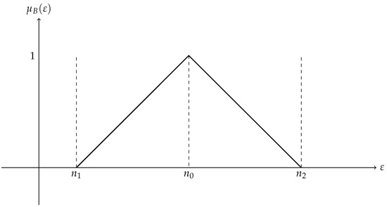
A triangle membership function distinguishes a triangular fuzzy set from other kinds of fuzzy sets. Three parameters determine the piece-wise linear membership function of a triangular fuzzy set: an upper limit , a peak (where the membership value is 1), and a lower limit . This is one way to express the triangle membership function. It is shown in Figure 1.
Figure 1.
Triangular fuzzy number.
Definition 3
([49]). The Generalized Mean Integration Value (GMIV) of a fuzzy number is a method used to defuzzify or obtain a crisp value from a fuzzy number. It is defined as
where and are inverse functions of B. indicates the optimism level and . A decision-making point of view is considered optimistic if , pessimistic if , and somewhat optimistic if .
Definition 4.
The left and right shape functions for the TNF of set B are and , respectively. After some simplifications, we have
For the TFN , defuz (B) is reduced to the real number .
2.1. Basic Model
This subsection presents the formulation of the predator–prey model with diseases in the predator population based on the following assumptions:
- The prey population exhibits a logistic growth pattern in the absence of predators. This growth is constrained by a carrying capacity and characterized by an inherent growth rate. The growth rate of the prey population declines as it approaches its carrying capacity.
- The disease is transmitted through direct contact between individuals. Specifically, the disease only affects the predator population and has no impact on the prey population.
- In this model, we assume that prey are less likely to be captured by predators as the prey population takes refuge and becomes inaccessible to the predators. Here, is the fraction of prey that is in refuge.
Following the work in [50] and considering these assumptions, the dynamics of the system with prey refuge and harvesting can be described as follows:
where X, Y, and Z represent the density of prey, susceptible predators, and infected predators, respectively. K represents the carrying capacity and r is the growth rate of the prey. The parameter represents the rate of prey consumption by susceptible predators, while is the rate of consumption of prey by diseased predators. The half-saturation constant is the prey population level at which predation is reduced to half of its maximum rate. The parameters and represent the conversion rates of prey into susceptible and infected predators, respectively. The parameter represents the natural death rate of susceptible predators. The parameter represents prey refuge. The parameter captures the disease transmission rate. The parameter represents the extra mortality rate in predators as a result of infection.
Generally, harvesting significantly affects the dynamics of the system. Here, it is applied to both susceptible and infected predators through the continuous functions and . Following the hypothesis of Clark [51], we assume here that harvesting in both classes of predators is based on the catch per unit of effort, which depends on the population stock levels. In this context, and are denoted as the catchability rates for susceptible and infected predators, respectively.
For simplicity, Model (4) can be converted into a non-dimensional form using these transformations:
After suitable simplification, we have
Here,
2.2. Fuzzy Model
The fuzzy model, which uses triangular fuzzy numbers for each parameter, is presented as follows:
where the triangular fuzzy numbers are defined as follows: , , , , , , , , , , .
The parameter values in the crisp, fuzzy, and defuzzified models are represented in Table 2.
Table 2.
Parameter values in the crisp, fuzzy, and defuzzified models.
2.3. Defuzzified Model
While fuzzy models are useful for incorporating uncertainty, practical applications often require crisp outputs. Defuzzification is the process of converting a fuzzy result into a single crisp value, which can be used for further analysis or decision-making.
The fuzzified system is then transformed into the defuzzified form using the graded mean defuzzification technique [49]. By applying the graded mean defuzzification method, the model is simplified into the following form:
Here, defuz represents the defuzzified/GMIV parameter. To convert fuzzy parameters into defuzzified parameters, we choose the optimistic scenario, i.e., , which assumes lower predation and better survival of prey. We show the defuzzified values in Table 2.
2.4. Basic Model Analysis
2.4.1. Equilibria
In this section, the local stability analysis of the equilibrium points in model (5) is examined by applying Jacobian matrix analysis. The system described in Equation (5) has the following equilibria:
where , , , , and is the positive solution to the following equation:
Here, the values of p, q, r, and s are given as follows:
Moreover, we have
and
2.4.2. Biological Significance of Reproduction Numbers
This section will elucidate the biological significance of reproduction numbers, as determined by local stability analysis of equilibrium points. The same method has been used to derive and analyze reproduction numbers as in [36]. For a more clear explanation of these reproduction numbers, we refer the reader to the works in [52,53]. Initially, is defined as follows:
This provides an explanation for the local stability of the equilibrium point , which reflects the predator’s efficiency in turning prey into predator growth. It shows that the predators are more effective in using the prey as food to increase its population size if is higher. Thus, the term represents the birth rate of the susceptible predators, and , denotes the rate of removal of the susceptible predators. Hence, can be interpreted as the average number of new susceptible predators produced during the lifetime of a susceptible predator, which can be interpreted as ecological reproduction. The term was originally developed and interpreted by Pilou [54] in an ecological context, representing the average number of prey that are converted to predator biomass during a predator’s lifetime. After that, Hethcote et al. [55] explained it in an eco-epidemiological model. The susceptible predator population increases and persists if , whereas it decreases and eventually goes extinct if . Also, is defined as follows:
Similarly, represents the birth rate of the infected predators and , denotes the rate of removal of the infected predators. Thus, can be interpreted as the disease reproduction number. If , the infected predator population grows and endures, whereas if , it declines and eventually becomes extinct. At , the reproduction number is
Here, denotes the growth rate of the infected predators due to predation. In addition, is the removal rate of infected predators; therefore, can be interpreted as the diseases reproduction number. The infected predator population can increase and persist if . The predator population becomes free of the disease if , and the number of infected predators decreases. At , the reproduction is
Similarly, is the birth rate of susceptible newborn predators and is the removal rate of susceptible predators; therefore, can be interpreted as the ecological reproduction number. The susceptible predator population can increase and persist if . The predator population becomes free of the disease if , and the number of susceptible predators decreases.
2.4.3. Investigation the Stability and Existence of Equilibrium Points
Here, we present some key results, while the complete analysis, including the bifurcation study, is provided in the Appendix A.
Theorem 1.
The zero equilibrium point always exhibits instability, showing that the system cannot stay in a state of total extinction. The axial equilibrium point is locally stable when and .
Theorem 2.
The epidemic free equilibrium point is locally stable if , where .
Theorem 3.
The endemic equilibrium point is locally stable if , where and .
Theorem 4.
The equilibrium point of the system (5) exists and it is locally asymptotically stable if
Lemma 1.
The system exhibits a Hoph-bifurcation when ϱ crosses the critical value , provided that the following three conditions are satisfied.
- 1.
- ,
- 2.
- ,
- 3.
- < ,
where , , and represent the coefficients of the characteristic cubic Equation (A1) at the interior equilibrium point.
3. Numerical Simulations
In this part, the spatiotemporal dynamics of the system will be studied. Extensive simulations were carried out using random values of parameters to validate theoretical findings and to investigate the effects of the main parameters such as transmission rate, prey refuge, and harvesting. Bifurcation analysis is also provided.
Firstly, for the crisp model (6), the populations of prey, susceptible predators, and infected predators exhibit oscillatory behavior for a set of parameters; Figure 2 is given as an example. Figure 2a is in crisp environment; using the same parameters as in Figure 2a, we determine that is and is , which shows instability of the system according to Theorem 1. Figure 2b is given as an example in an uncertain environment. A phase portrait of the system is plotted in Figure 2c,d in both crisp and fuzzy environments.
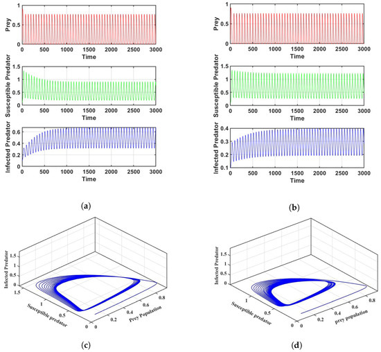
Figure 2.
Co-existence of prey, susceptible predators, and infected predators for the parameter values in Table 2: (a) Frequency of three populations in a crisp environment, (b) Frequency of three populations in a fuzzy environment, (c) Phase portrait of the system in a crisp environment, (d) Phase portrait of the system in a fuzzy environment.
Prey refuge is one of the key elements influencing the dynamics between prey and predator populations. If we change the parameter to be 0.35 and keep the other parameters the same as in Figure 2a, the system enters into a stable position, which can be seen in Figure 3a.
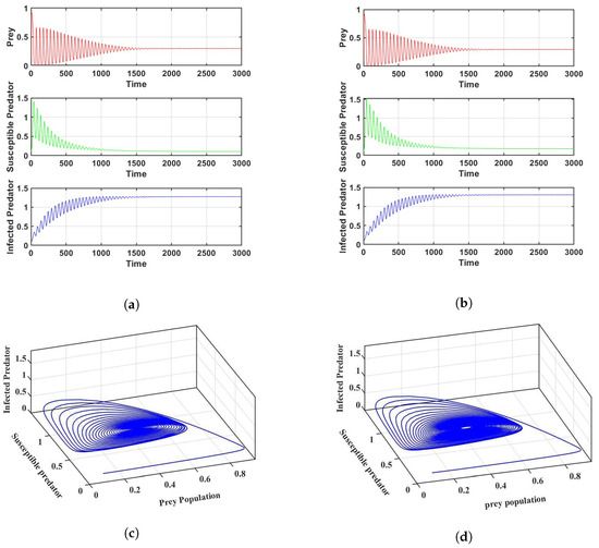
Figure 3.
Stability of the systems for the parameter values in Table 2: (a) For in a crisp environment and (b) For in a fuzzy environment. (c) Phase portrait of the system corresponding to (a,d) Phase portrait of the system corresponding to (b).
Similarly, the system enters a stable position when the parameter is 0.348 and the other parameters remain the same as in Figure 2b in a fuzzy environment, as shown in Figure 3b. The corresponding phase portraits are shown in Figure 3c,d in both crisp and fuzzy environments. Using the values of the parameters in Figure 3a, we determine that is , which verifies the conclusion of Theorem 2. It is interesting that the system experiences Hopf bifurcations at . The bifurcation diagram of the parameter is depicted in Figure A1a–c. In Figure A1a–c we can see that for a small value of , the system cannot be stabilized. However, with an increase in the parameter , the system stabilizes after crossing a critical threshold. This result verifies the conclusion of Lemma 1. However, the parameter first stabilizes the system, then destabilizes it after reaching a certain threshold. Figure A1d–f is given as an example.
Secondly, the effects of prey refuge () on the dynamics of the system were studied. The results show that for small values of , the infected predators tend toward extinction, while the susceptible predators and prey remain with high oscillations. Figure 4 is given as an example.
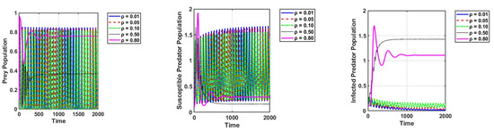
Figure 4.
Effect of prey refuge on the dynamics of the system. The parameter values are the same as those in Table 2.
We can see that when crosses the threshold value, the system becomes stable, as shown in Figure 4. The phase portrait for different values of is depicted in Figure 5 in crisp and fuzzy environments. As we can see in Figure 5, the system becomes stable for larger values of .
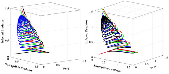
Figure 5.
Phase portraits of systems for different parameter settings in a crisp environment and a fuzzy environment, respectively. The values of prey refuge in a crisp environment for black, blue, green, and red are 0.35, 0.4, 0.45, and 0.5, respectively. In a fuzzy environment, the corresponding values are 0.0348, 0.38, 0.448, and 0.48. The other parameter values are the same as those in Table 2.
Thirdly, we modify the values of and to investigate how harvesting affects the dynamics of the system. We can see that the infected predators go extinct, while the susceptible predators and prey exist with strong oscillations in certain values of harvesting of susceptible predators. This is because harvesting causes a drop in predation pressure and an increase in predator mortality, which naturally leads to an increase in the prey population. Setting = 0.10 and keeping the other parameters unchanged, as in Figure 2a, the reproduction number is . This shows that the diseases are extinct, as can be observed in Figure 6.
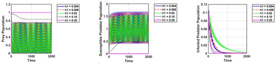
Figure 6.
Effect of harvesting of susceptible predators on the dynamics of the system. The parameter values are the same as those in Table 2, except the conversion rate of prey into infected predators .
Furthermore, we observe that the populations of susceptible predators and prey exhibit oscillatory behavior, while the population of infected predators goes extinct when the infected predators are harvested, as shown in Figure 7.
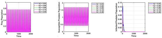
Figure 7.
Effect of harvesting of the infected population on the dynamics of the system. The parameter values are the same as those in Table 2.
In a fuzzy environment, this phenomenon can also be observed, with greater oscillations between the susceptible predator and the prey. Setting = 0.03 and keeping other parameters unchanged, as in Figure 2a, the reproduction numbers are as follows: is and is . This shows that the diseases are eradicated.
Lastly, if both harvesting of infected predators and prey refuge increase, the dynamics of the system undergo significant changes, as shown in Figure 8a–c. An increased rate of harvesting of infected predators reduces the number of infected predators, thus causing a reduction in infection transmission and consequently preventing overexploitation to prey. While a small prey refuge offers very little protection from predation, it allows the prey population to build up without excessive depletion. This, in turn, allows the prey population to flourish and keeps the susceptible predator population low. The infected predator population goes extinct due to the synergistic effect of harvesting and the loss of available hosts for the disease. The effects of increasing the harvesting of susceptible predators while keeping the prey refuge small are also significant, and Figure 8d–f is given as an example. The conclusion drawn is that the judicious use of prey refuge and harvesting can be effective strategies for preventing the spread of disease.
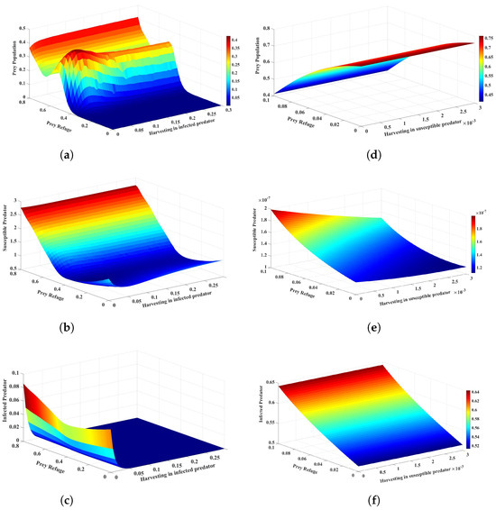
Figure 8.
The effects of variation in the harvesting of infected predators and prey refuge on the dynamics of the system are represented in (a–c). The harvesting of susceptible predators and the prey refuge on the dynamics of system are represented in (d–f). The other parameter values are the same as those in Table 2.
4. Discussion and Conclusions
In this paper, a deterministic model of the predator–prey system is constructed with diseases in the predator population. Additionally, fuzzy analysis is used to address the uncertain environment. The primary goal of this research is to demonstrate how harvesting and prey refuge can be effectively used to control the spread of diseases in the predator population. The stability of the equilibria of the system, Hopf bifurcations, and basic reproduction numbers were analyzed. Particularly, this study focused on the combined effect of prey refuge and harvesting on the dynamics of the system.
The hiding behavior of the prey strongly influences the dynamics of system. Numerous authors concluded that the dynamics of predator–prey relationships are stabilized by the pressure of prey refuge [28,29,31]. Our results are different in the context of disease in the predator population. We noticed that the prey refuge had both stabilizing and extinction effects on the population of infected predators. We observed that when we decreased the value of the prey refuge parameter (), more prey were exposed. Therefore, susceptible predators become dominant, as infection diminishes the ability of infected predators to catch prey. Therefore, the infected predator population tends towards extinction, while the prey and susceptible predator populations experience intense fluctuations. When we increase the value of the prey refuge parameter (), more prey are in the hidden refuge. Therefore, the susceptible predator population cannot grow too fast. As a result, all populations, including prey, susceptible predators, and infected predators, stabilize significantly. This suggests that prey refuge plays an important role in stabilizing the system and controlling disease in the predator population with suitable harvesting levels.
Harvesting causes a drop in prey density and an increase in predator mortality, which naturally boosts prey populations. According to some existing studies, harvesting can be a useful strategy for limiting the spread of disease [36,39]. However, our findings present slightly different perspectives on this issue. Our results indicate that low harvesting of the susceptible predators leads to the extinction of the infected predators, but the prey and susceptible predators undergo severe oscillations. However, with a further increase in the intensity of harvesting, both susceptible and infected predator populations go to extinct, and the prey population is stabilized. In contrast, harvesting in the infected predator does not produce the same outcome. Regardless of the intensity of harvesting imposed on the infected predators, only this population goes extinct, while the prey and susceptible predators coexist with severe oscillations. The findings suggest that a carefully planned harvesting strategy combined with prey refuge can be an effective strategy for disease control in predator populations.
In our study, we have constructed a model in a fuzzy environment, which considers uncertainties in parameters. It is clear that at certain levels of harvesting, both prey and susceptible predator populations thrive robustly, while the infected predators go extinct. The fuzzy model effectively captures the vagueness in the parameters and thus provides a more realistic depiction of the behavior of the system.
Targeted harvesting is crucial to population dynamics and ecosystem sustainability in sponge fisheries in Florida (USA) [56]. Their research further supports the notion that harvesting can be a useful strategy for population management by demonstrating that selective and careful harvesting has minimal impact on non-target species. We are confident that studying such systems will provide valuable insights derived from our mathematical model.
To further enhance this research, the existing model may be extended by incorporating additional phenomena, such as time-varying or nonlinear harvesting schedules in place of fixed rates, and by allowing prey refuge to depend dynamically on prey density. The inclusion of stochastic forcing or environmental fluctuations could yield deeper insights into species persistence and extinction under more realistic conditions. Furthermore, introducing additional prey or predator species into the system may increase ecological stability and render the theoretical predictions more closely aligned with real-world scenarios.
Author Contributions
Conceptualization, I.A., H.Z., G.Z., A.T. and L.W.; Methodology, I.A., H.Z. and J.-J.T.; Validation, H.Z., G.Z., A.T. and J.-J.T.; Formal analysis, A.T., L.W. and J.-J.T.; Investigation, I.A., H.Z., G.Z., A.T. and L.W.; Resources, G.Z. and L.W.; Data curation, J.-J.T.; Writing—original draft, I.A. and A.T.; Visualization, I.A. and J.-J.T.; Supervision, H.Z. All authors have read and agreed to the published version of the manuscript.
Funding
This work was supported by the National Natural Science Foundations of China (No. 32271554) and the Guangdong Basic and Applied Basic Research Foundation (No. 2023A1515011501).
Data Availability Statement
The original contributions presented in this study are included in the article. Further inquiries can be directed to the corresponding authors.
Conflicts of Interest
The authors declare no conflicts of interest.
Appendix A. Stability Analysis of Equilibrium Points
The Jacobian matrix of System (5) is given as follows:
Proof of Theorem 1.
The zero equilibrium point is always unstable. It is easy to see that when is substituted into the Jabobian matrix, the resulting matrix has an eigenvalue of 1. The Jacobian matrix at is given as follows:
The eigenvalues of the Jacobian matrix at this axial equilibrium point are as follows:
Hence, is stable if and . Then, we can see and . □
Proof of Theorem 2.
The Jacobian matrix at is given as follows:
It is obvious that is one of the eigenvalues of the Jacobian matrix. The characteristic equation below for the sub-matrix can be solved to determine the remaining eigenvalues
where
and
The equilibrium point exhibits local stability, which requires , and . From it, we have . □
Proof of Theorem 3.
Now, the Jacobian matrix at can be expressed as follows:
The term is one of the eigenvalues of the Jacobian matrix. The remaining eigenvalues can be found by solving the quadratic equation below, which is generated from the sub-matrix
where
and
The equilibrium point is locally stable if it holds the conditions , and , which implies . □
Proof of Theorem 4.
The Jacobian matrix at equilibrium point is expressed as follows:
Here,
and the characteristic cubic equation of the Jacobian matrix, evaluated at the equilibrium point , is shown as
with . According to the Routh–Hurwitz condition, the local stability of the equilibrium point requires that , , and . □

Figure A1.
Bifurcation diagram for in (a–c) and in (d–f). The other parameters remain the same as in Table 2.
Figure A1.
Bifurcation diagram for in (a–c) and in (d–f). The other parameters remain the same as in Table 2.

Proof of Lemma 1.
Let the interior equilibrium point be asymptotically stable. We wish to determine if changing any one of the parameters will cause to become unstable. To analyze the Hopf-bifurcation of system (5), can be selected as a bifurcation parameter. We conduct a test to determine whether there is a crucial number that satisfies the following:
Hence, for , the characteristic Equation (A1) should be
Therefore, Equation (A2) has the following eigenvalues:
To observe the Hopf-bifurcation at , we need to verify the transversality criterion:
For all , the general roots will be
We will prove the transversality condition
Putting into Equation (A2) and performing differentiation, we obtain
where
For , , we get
For in Equation (A3), we have
and
Hence, the transverse conditions hold, and Hopf-bifurcation occurs at . □
References
- Sintunavarat, W.; Turab, A. Mathematical analysis of an extended SEIR model of COVID-19 using the ABC-fractional operator. Math. Comput. Simul. 2022, 198, 65–84. [Google Scholar] [CrossRef]
- Turab, A.; Shafqat, R.; Muhammad, S.; Shuaib, M.; Khan, M.F.; Kamal, M. Predictive modeling of hepatitis B viral dynamics: A caputo derivative-based approach using artificial neural networks. Sci. Rep. 2024, 14, 21853. [Google Scholar] [CrossRef]
- Paseka, R.E.; White, L.A.; de Waal, D.B.V.; Strauss, A.T.; González, A.L.; Everett, R.A.; Peace, A.; Seabloom, E.W.; Frenken, T.; Borer, E.T. Disease-mediated ecosystem services: Pathogens, plants, and people. Trends Ecol. Evol. 2020, 35, 731–743. [Google Scholar] [CrossRef] [PubMed]
- Keesing, F.; Belden, L.K.; Daszak, P.; Dobson, A.; Harvell, C.D.; Holt, R.D.; Hudson, P.; Jolles, A.; Jones, K.E.; Mitchell, C.E.; et al. Impacts of biodiversity on the emergence and transmission of infectious diseases. Nature 2010, 468, 647–652. [Google Scholar] [CrossRef] [PubMed]
- Anderson, R.M.; May, R.M. The invasion, persistence and spread of infectious diseases within animal and plant communities. Philos. Trans. R. Soc. Lond. Biol. Sci. 1986, 314, 533–570. [Google Scholar] [CrossRef]
- Lotka, A.J. Elements of Physical Biology; Williams and Wilkins: Baltimore, MD, USA, 1925. [Google Scholar] [CrossRef]
- Volterra, V. Fluctuations in the abundance of a species considered mathematically. Nature 1927, 119, 12–13. [Google Scholar] [CrossRef]
- Kermack, W.O.; McKendrick, A.G. A contribution to the mathematical theory of epidemics. Proc. R. Soc. 1927, 115, 700–721. [Google Scholar] [CrossRef]
- Zhang, H.; Xu, G.J.; Sun, H. Biological control of a predator–prey system through provision of an infected predator. Int. J. Biomath. 2018, 11, 1850105. [Google Scholar] [CrossRef]
- Xiang, A.; Wang, L. Boundedness and stabilization in a predator–prey model with prey-taxis and disease in predator species. J. Math. Anal. Appl. 2023, 522, 126953. [Google Scholar] [CrossRef]
- Richards, R.L.; Elderd, B.D.; Duffy, M.A. Unhealthy herds and the predator–spreader: Understanding when predation increases disease incidence and prevalence. Ecol. Evol. 2023, 13, e9918. [Google Scholar] [CrossRef]
- Wilmers, C.C.; Post, E.; Peterson, R.O.; Vucetich, J.A. Predator disease out-break modulates top-down, bottom-up and climatic effects on herbivore population dynamics. Ecol. Lett. 2006, 9, 383–389. [Google Scholar] [CrossRef] [PubMed]
- Gulland, F.M.D. The impact of infectious diseases on wild animal populations: A review. Ecol. Infect. Dis. Nat. Popul. 1995, 1, 20–51. [Google Scholar] [CrossRef]
- Collyer, B.S.; Anderson, R.M. Probability distributions of helminth parasite burdens within the human host population following repeated rounds of mass drug administration and their impact on the transmission breakpoint. J. R. Soc. Interface 2021, 18, 20210200. [Google Scholar] [CrossRef]
- Byers, J.E. Marine parasites and disease in the era of global climate change. Annu. Rev. Mar. Sci. 2021, 13, 397–420. [Google Scholar] [CrossRef]
- Sapp, S.G.H.; Rascoe, L.N.; Wilkins, P.P.; Handali, S.; Gray, E.B.; Eberhard, M.; Woodhall, D.M.; Montgomery, S.P.; Bailey, K.L.; Lankau, E.W.; et al. Baylisascaris procyonis roundworm seroprevalence among wildlife rehabilitators, United States and Canada, 2012–2015. Emerg. Infect. Dis. 2016, 22, 2128. [Google Scholar] [CrossRef]
- Bauer, C. Baylisascariosis—Infections of animals and humans with ‘unusual’ roundworms. Vet. Parasitol. 2013, 193, 404–412. [Google Scholar] [CrossRef]
- Flegr, J.; Prandota, J.; Sovičková, M.; Israili, Z.H. Toxoplasmosis–a global threat. Correlation of latent toxoplasmosis with specific disease burden in a set of 88 countries. PLoS ONE 2014, 9, e90203. [Google Scholar] [CrossRef]
- McNair, J.N. The effects of refuges on predator-prey interactions: A reconsideration. Theor. Popul. Biol. 1986, 29, 38–63. [Google Scholar] [CrossRef]
- Gilliam, J.F.; Fraser, D.F. Habitat selection under predation hazard: Test of a model with foraging minnows. Ecology 1987, 68, 1856–1862. [Google Scholar] [CrossRef]
- Sagrario, G.; Ángeles, M.A.D.L.; Balseiro, E.; Ituarte, R.; Spivak, E. Macrophytes as refuge or risky area for zooplankton: A balance set by littoral predacious macroinvertebrates. Freshw. Biol. 2009, 54, 1042–1053. [Google Scholar] [CrossRef]
- Chen, W.C.; Yu, H.G.; Dai, C.J.; Guo, Q.; Liu, H.; Zhao, M. Stability and bifurcation in a predator–prey model with prey refuge. J. Biol. Syst. 2023, 31, 417–435. [Google Scholar] [CrossRef]
- Chatterjee, A.; Abbasi, M.A.; Venturino, E.; Zhen, J.; Haque, M. A predator–prey model with prey refuge: Under a stochastic and deterministic environment. Nonlinear Dyn. 2024, 112, 13667–13693. [Google Scholar] [CrossRef]
- Turab, A.; Sintunavarat, W. On the solutions of the two preys and one predator type model approached by the fixed point theory. Sādhanā 2020, 45, 211. [Google Scholar] [CrossRef]
- Turab, A.; Sintunavarat, W. On a solution of the probabilistic predator–prey model approached by the fixed point methods. J. Fixed Point Theory Appl. 2020, 22, 64. [Google Scholar] [CrossRef]
- Sharma, S.; Samanta, G.P. A Leslie–Gower predator–prey model with disease in prey incorporating a prey refuge. Chaos Solitons Fractals 2015, 70, 69–84. [Google Scholar] [CrossRef]
- Belew, B.; Yiblet, Y. Dynamical analysis of a Modified Leslie–Gower Predator-prey model with disease in prey incorporating a prey refuge and treatment. Int. J. Biomath. 2024, 21, 2450051. [Google Scholar] [CrossRef]
- Pradeep, M.S.; Nandha, G.T.; Sibabalan, M.; Yasotha, A. Bifurcation and Dynamic Analyses of a Diseased Predator-prey Model With Prey Refuge. Int. J. Appl. Comput. Math. 2023. [Google Scholar] [CrossRef]
- Lazaar, O.; Serhani, M. Stability and optimal control of a prey–predator model with prey refuge and prey infection. Int. J. Dyn. Control 2023, 11, 1934–1951. [Google Scholar] [CrossRef]
- Khan, M.; Sen, P.; Samanta, S. Stability and bifurcation analysis of an eco-epidemiological model with prey refuge. Nonlinear Stud. 2024, 31, 183–209. [Google Scholar] [CrossRef]
- Chauhan, R.P.; Singh, R.; Kumar, A.; Thakur, N.K. Role of prey refuge and fear level in fractional prey–predator model with anti-predator. J. Comput. Sci. 2024, 81, 102385. [Google Scholar] [CrossRef]
- Clark, C.W. Mathematical models in the Economics of Renewable Resources. SIAM Rev. 1979, 21, 81–99. [Google Scholar] [CrossRef]
- Hannesson, R. Optimal harvesting of ecologically interdependent fish species. J. Environ. Econ. Manag. 1983, 10, 329–345. [Google Scholar] [CrossRef]
- Ragozin, D.L.; Brown, G., Jr. Harvest policies and nonmarket valuation in a predator—Prey system. J. Environ. Econ. Manag. 1985, 12, 155–168. [Google Scholar] [CrossRef]
- Meng, X.Y.; Qin, N.N.; Huo, H.F. Dynamics analysis of a predator–prey system with harvesting prey and disease in prey species. J. Biol. Dyn. 2018, 12, 342–374. [Google Scholar] [CrossRef] [PubMed]
- Das, K.P. A study of harvesting in a predator–prey model with disease in both populations. Math. Methods Appl. Sci. 2016, 39, 2853–2870. [Google Scholar] [CrossRef]
- Jana, S.; Guria, S.; Das, U.; Kar, T.K.; Ghorai, A. Effect of harvesting and infection on predator in a prey–predator system. Nonlinear Dyn. 2015, 81, 917–930. [Google Scholar] [CrossRef]
- Themairi, A.A.; Alqudah, M.A. Predator-prey model of Holling-type II with harvesting and predator in disease. Ital. J. Pure Appl. Math. 2020, 43, 744–753. [Google Scholar]
- Das, D.K.; Das, K.; Kar, T.K. Dynamical behaviour of infected predator–prey eco-epidemics with harvesting effort. Int. J. Appl. Comput. Math. 2021, 7, 1–27. [Google Scholar] [CrossRef]
- Zadeh, L.A. The role of fuzzy logic in modeling, identification and control. In Fuzzy Sets, Fuzzy Logic, and Fuzzy Systems: Selected Papers; World Scientific: Waltham, MA, USA, 1996; pp. 783–795. [Google Scholar] [CrossRef]
- Gonzalez, A.; Pons, O.; Vila, M.A. Dealing with uncertainty and imprecision by means of fuzzy numbers. Int. J. Approx. Reason. 1999, 21, 233–256. [Google Scholar] [CrossRef][Green Version]
- Oberguggenberger, M.; Pittschmann, S. Differential equations with fuzzy parameters. Math. Comput. Model. Dyn. Syst. 1999, 5, 181–202. [Google Scholar] [CrossRef]
- Yu, X.; Yuan, S.; Zhang, T. About the optimal harvesting of a fuzzy predator–prey system: A bioeconomic model incorporating prey refuge and predator mutual interference. Nonlinear Dyn. 2018, 94, 2143–2160. [Google Scholar] [CrossRef]
- Das, S.; Mahato, P.; Mahato, S.K. Disease control prey–predator model incorporating prey refuge under fuzzy uncertainty. Model. Earth Syst. Environ. 2021, 7, 2149–2166. [Google Scholar] [CrossRef]
- Das, S.; Mahato, P.; Mahato, S.K. A prey predator model in case of disease transmission via pest in uncertain environment. Differ. Equ. Dyn. Syst. 2023, 31, 457–483. [Google Scholar] [CrossRef]
- Kumar, A.; Malik, M.; Kang, Y. Dynamics of eco-epidemiological predator-prey model in fuzzy environment. Int. J. Biomath. 2025, 2550071. [Google Scholar] [CrossRef]
- Kaladhar, K.; Singh, K. Stability Analysis of a TS Prey-Predator Model with Disease in both Species using Fuzzy Impulsive Control. J. Environ. Account. Manag. 2024, 12, 231–247. [Google Scholar] [CrossRef]
- Ahmad, M.Z.; Hasan, M.K. Modeling of biological populations using fuzzy differential equations. In International Journal of Modern Physics: Conference Series; World Scientific Publishing Company: Waltham, MA, USA, 2012; Volume 9, pp. 354–363. [Google Scholar] [CrossRef]
- Chiao, K.P. Ranking interval type 2 fuzzy sets using parametric graded mean integration representation. In Proceedings of the 2016 International Conference on Machine Learning and Cybernetics (ICMLC), Jeju, Republic of Korea, 10–13 July 2016; Volume 2, pp. 606–611. [Google Scholar] [CrossRef]
- Das, K.P. Proper predation and disease transmission in predator population stabilize predator–prey oscillations. Differ. Equ. Dyn. Syst. 2020, 28, 295–313. [Google Scholar] [CrossRef]
- Clark, C.W. Mathematical Bioeconomics: The Optimal Management Resources; John Wiley & Sons: Hoboken, NJ, USA, 1976. [Google Scholar]
- Hsieh, Y.H.; Hsiao, C.K. Predator–prey model with disease infection in both population. Math. Med. Biol. J. IMA 2008, 25, 247–266. [Google Scholar] [CrossRef]
- Kooi, B.W.; van Voorn, G.A.; Das, K.P. Stabilization and complex dynamics in a predator–prey model with predator suffering from an infectious disease. Ecol. Complex. 2011, 8, 113–122. [Google Scholar] [CrossRef]
- Pielou, E.C. An Introduction to Mathematical Ecology; Wiley: Hoboken, NJ, USA, 1969. [Google Scholar] [CrossRef]
- Hethcote, H.W.; Wang, W.; Han, L.; Ma, Z. A predator–prey model with infected prey. Theor. Popul. Biol. 2004, 66, 259–268. [Google Scholar] [CrossRef]
- Behringer, M.J.B.I.V.D.C.; Valentine, M.M. Commercial sponge fishery impacts on the population dynamics of sponges in the Florida Keys, FL (USA). Fish. Res. 2017, 190, 113–121. [Google Scholar] [CrossRef]


Disclaimer/Publisher’s Note: The statements, opinions and data contained in all publications are solely those of the individual author(s) and contributor(s) and not of MDPI and/or the editor(s). MDPI and/or the editor(s) disclaim responsibility for any injury to people or property resulting from any ideas, methods, instructions or products referred to in the content. |
© 2025 by the authors. Licensee MDPI, Basel, Switzerland. This article is an open access article distributed under the terms and conditions of the Creative Commons Attribution (CC BY) license (https://creativecommons.org/licenses/by/4.0/).