Review

Review of Physics-Informed Neural Networks: Challenges in Loss Function Design and Geometric Integration

by
Sergiy Plankovskyy
1,
Yevgen Tsegelnyk
1,*,
Nataliia Shyshko
1,
Igor Litvinchev
2,
Tetyana Romanova
3,4 and
José Manuel Velarde Cantú
5,*
1
School of Energy, Information and Transport Infrastructure, O. M. Beketov National University of Urban Economy in Kharkiv, 61002 Kharkiv, Ukraine
2
Faculty of Mechanical and Electrical Engineering, Autonomous University of Nuevo Leon, Monterrey 66455, Mexico
3
Leeds University Business School, University of Leeds, Leeds LS2 9JT, UK
4
Anatolii Pidhornyi Institute of Power Machines and Systems of the National Academy of Sciences of Ukraine, 61046 Kharkiv, Ukraine
5
Department of Industrial Engineering, Technological Institute of Sonora (ITSON), Navojoa 85800, Mexico
*
Authors to whom correspondence should be addressed.
Mathematics 2025, 13(20), 3289; https://doi.org/10.3390/math13203289
Submission received: 8 September 2025 / Revised: 2 October 2025 / Accepted: 7 October 2025 / Published: 15 October 2025

Abstract

Physics-Informed Neural Networks (PINNs) represent a transformative approach to solving partial differential equation (PDE)-based boundary value problems by embedding physical laws into the learning process, addressing challenges such as non-physical solutions and data scarcity, which are inherent in traditional neural networks. This review analyzes critical challenges in PINN development, focusing on loss function design, geometric information integration, and their application in engineering modeling. We explore advanced strategies for constructing loss functions—including adaptive weighting, energy-based, and variational formulations—that enhance optimization stability and ensure physical consistency across multiscale and multiphysics problems. We emphasize geometry-aware learning through analytical representations—signed distance functions (SDFs), phi-functions, and R-functions—with complementary strengths: SDFs enable precise local boundary enforcement, whereas phi/R capture global multi-body constraints in irregular domains; in practice, hybrid use is effective for engineering problems. We also examine adaptive collocation sampling, domain decomposition, and hard-constraint mechanisms for boundary conditions to improve convergence and accuracy and discuss integration with commercial CAE via hybrid schemes that couple PINNs with classical solvers (e.g., FEM) to boost efficiency and reliability. Finally, we consider emerging paradigms—Physics-Informed Kolmogorov–Arnold Networks (PIKANs) and operator-learning frameworks (DeepONet, Fourier Neural Operator)—and outline open directions in standardized benchmarks, computational scalability, and multiphysics/multi-fidelity modeling for digital twins and design optimization.

1. Introduction

In recent years, physics-informed neural networks (PINNs) have become one of the leading approaches for solving boundary value problems described by partial differential equations (PDEs). This is since this approach, proposed by Raissi et al. [1], largely addressed issues that were inherent in the neural networks applied to such problems before the advent of PINNs. First, solutions obtained using conventional neural networks often did not comply with physical laws, because they did not account for the structure of the differential equations, boundaries, and initial conditions. Therefore, the results could be non-physical, unstable, or unsuitable for interpretation. Second, effective training of conventional neural network models required large volumes of data—numerical or experimental. This limited the application of neural networks to practical problems where obtaining such data is complicated, expensive, or fundamentally restricted.
The core idea of PINNs is to embed physical laws into the neural network training process by representing known differential equations as a component of the loss function. The network simultaneously minimizes errors between predictions or experimental data and the residuals of the governing equations and boundary conditions at selected points. A key prerequisite for the effective application of PINNs is the ability to define loss function components related to PDE residuals and boundary conditions using automatic differentiation available in modern machine learning frameworks (e.g., TensorFlow [2] and PyTorch [3]).
These advantages have sparked intense interest in applying PINNs, and the results of numerous studies have shown that this interest is justified, with PINNs proving effective in modeling various physical processes—fluid and gas dynamics (e.g., reviews by Cai et al. [4], Sharma et al. [5]), structural mechanics (e.g., reviews by Hu et al. [6], Faroughi et al. [7], Herrmann and Kollmannsberger [8]), heat conduction (e.g., reviews by Karniadakis et al. [9], Du and Lu [10]), electromagnetism and optics (e.g., review by Abdelraouf et al. [11]), and more. Cai et al. [4] note that PINNs are particularly effective for solving inverse problems where some data is available from multimodal measurements, for which traditional finite element methods (FEM) are often excessively costly and inefficient [12]. Meanwhile, Sharma et al. [5] point out that, despite significant progress in fluid flow problems, unresolved challenges remain. Specifically, PINN models have been tested only on specific problem configurations and datasets. To evaluate the effectiveness of developed algorithms, they must be validated on standardized datasets established by the community, as is performed for image recognition tasks. Additionally, Sharma et al. [5] suggest that, for robust PINN training, it is advisable to start with simpler problems and progressively train on more complex configurations. They also demonstrated that PINNs are better suited for modeling sequences of states rather than predicting spatiotemporal solutions from initial and boundary conditions. Sharma et al. [5] note that in real problems, PINNs face issues related to the complex geometry of computational domains and multiphysics phenomena. In reviews concerning solid mechanics [6,7], it is noted that, in many cases, PINNs eliminate the need for computationally expensive mesh generation, facilitating work with irregular and moving computational domains. The authors also indicate that PINNs are effective in inverse problems with sparse, unlabeled, and noisy data. However, when assessing the prospects for PINN development, Hu et al. [6] indicate that the problem of weighting PDE residuals in multiscale problems needs to be addressed, and for multiphysics problems, it is advisable to combine the loss function into a single equation. Karniadakis et al. [9] also identify inverse problems as the most promising for PINN applications and emphasize the necessity of domain decomposition for problems with complex geometries. Like the review by Sharma et al. [5], they underscore the urgent need for standardized benchmarks to evaluate various algorithms and the development of new mathematical frameworks for next-generation neural network modeling methods.
Du and Lu [10] explored promising directions for PINN development, focusing on improving thermal management in electronics and battery systems. In addition to the points mentioned above, they highlighted the need to account for variable thermal properties and complex heat transfer mechanisms when modeling intricate problems [13].
Abdelraouf et al. [11] emphasize the transformative impact of PINNs on the design of electromagnetic and nanophotonic systems, focusing on their advantages in rapid optimization, accurate modeling, and maintaining physical consistency with limited data. However, they note that integrating physical laws into these problems creates stiff, nonlinear loss function landscapes, complicating convergence, particularly for multiscale and multidimensional systems. Balancing residuals (physical and data-driven) remains a persistent challenge requiring task-specific tuning, while computational costs limit PINN applications for geometrically complex systems. The authors propose addressing these issues through adaptive PINN architectures with dynamic loss weighting, domain decomposition, and multifidelity modeling. They also stress the need for interdisciplinary integration with existing industrial solutions and the coupling of modeling with experimental validation.
The scope of PINN application for modeling processes of various natures is rapidly developing. The potential of PINN has been demonstrated in a wide range of biomedical applications, including systems biology, systems pharmacology, biomechanics, and epidemiology. By integrating biophysical laws with data-driven learning, PINN offers a powerful foundation for solving complex problems in these fields. The interest in modeling diverse processes using PINN-based algorithms is growing rapidly, as evidenced by the exponential increase in publications. This trend is illustrated in Figure 1, which shows the number of articles indexed in Scopus as of August 2025 containing the term PINN in the Abstract or Keywords. This growth reflects the broad recognition of PINNs’ potential within the scientific and engineering communities.
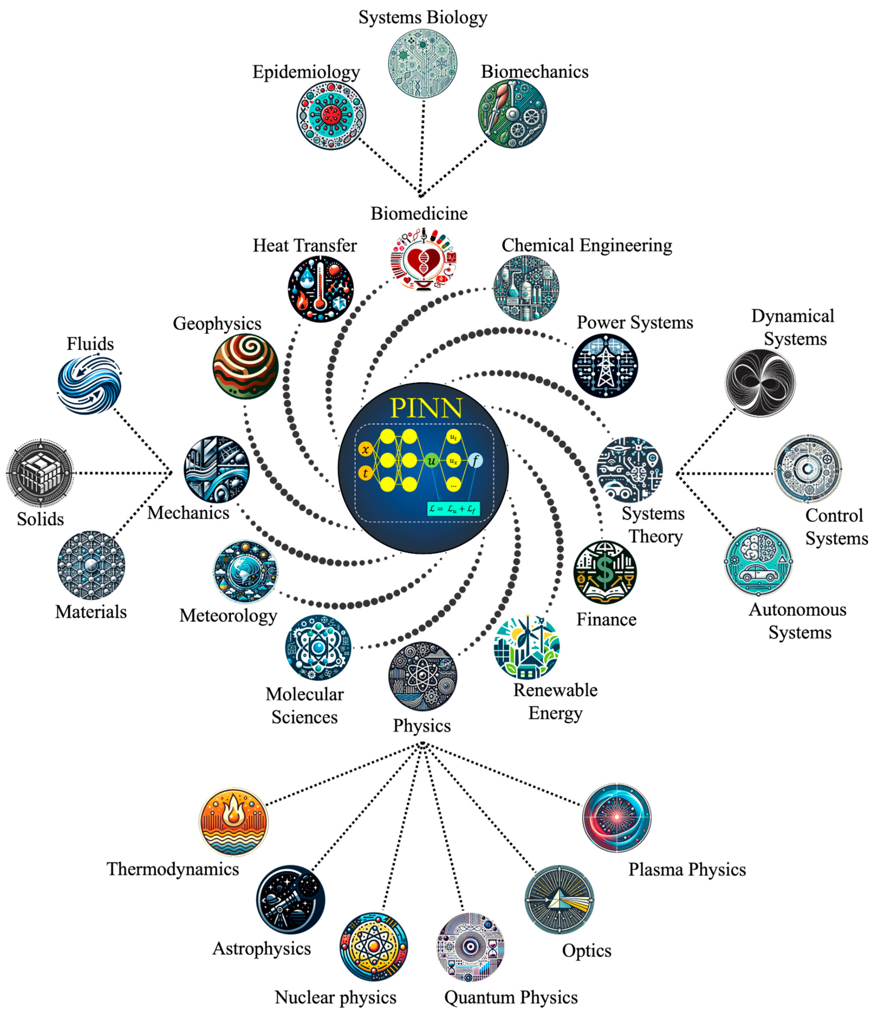
Figure 2 illustrates the existing applications of such PINNs across various scientific domains [14]. However, this review focuses on the use of PINNs in engineering modeling problems. The successes of applying artificial intelligence (AI) in this field, demonstrated in an increasing number of studies, have prompted leading CAD/CAE system developers (e.g., ANSYS, Autodesk, Siemens, Dassault Systèmes) to begin integrating AI tools, particularly PINNs, into their commercial software packages. Recent reviews by Khanolkar et al. [15], Uulu et al. [16], Montáns et al. [17], and Zhao et al. [18] indicate that AI integration in CAE occurs at three interconnected levels: supporting the workflow (geometry, meshing, pre- and post-processing), simulation and optimization methods (from reduced-order models to PINNs and operator neural networks), and applications in specific domains. However, despite their recognized potential, integrating PINNs with CAE packages faces challenges, including the need for computational resource optimization, ensuring result interpretability, and compatibility with existing CAD system formats.
Review papers indicate that deep learning methods significantly enhance the recovery of complex geometries and automate meshing, simplify the definition of constitutive models, accelerate solutions through surrogates and PINNs, and enable efficient post-processing [16,17,18]. However, limitations in data and training are noted: while PINNs can operate with minimal data, the lack of high-quality validation data in industrial CAE calculations leads to inaccuracies, particularly for complex problems—nonlinear, multiscale, and multiphysics.
It is noted that practical applications may encounter issues with accuracy and stability: in industrial contexts, without pre-training, PINNs often fail to achieve desired accuracy and may significantly underperform traditional solvers in terms of solution time for forward-modeling problems due to difficulties in hyperparameter tuning [18,19]. Applying PINNs in industrial computational packages requires intensive computations to balance data and physical constraint losses, complicating their integration into commercial packages without significant resource optimization [20]. This underscores the need for research into more efficient methods for integrating diverse data types into PINN-based algorithms. When combining PINNs with traditional solvers, issues with interpretability and uncertainty arise: PINNs are difficult to interpret, and assessing result uncertainty is critical for CAE, where errors can have serious consequences [21]. This necessitates additional extensions to ensure result reliability. Finally, integrating PINNs with CAE may pose compatibility issues with existing solvers [22]. Ensuring compatibility with existing CAD system geometry transfer formats remains a challenge.
It should be noted that neural networks, including PINNs, are sometimes viewed as “black boxes” that produce results through a process that is not fully controllable. The conservative nature of the industrial design community complicates the adoption of such approaches, particularly in tasks involving critical systems (e.g., critical infrastructure, nuclear energy, aviation). A promising solution is hybrid approaches, where PINNs are used in conjunction with the FEM, with the final calculation controllably performed by FEM solvers. Recent reviews (e.g., Nath et al. [23], Li et al. [24]) confirm that such combined approaches, when using pre-trained networks, significantly (by orders of magnitude) reduce the time required to obtain modeling results, which is critical for design, optimization, and digital twin construction problems.
Considering the features related to AI integration with engineering modeling packages, there is a need to review and analyze research related to PINNs, focusing on the challenges outlined above. While existing reviews summarize key aspects of PINN development, these issues are not fully addressed.
The review by Toscano et al. [14] provides a broad overview of recent algorithmic developments and covers a wide range of PINN applications across various scientific disciplines. The reviews by Cuomo et al. [25] and Farea et al. [26] focus primarily on PINN methodology and applications in different fields, with less emphasis on algorithmic improvements. The review by Raissi et al. [27] provides a concise overview of PINNs and their extensions, with an example of data-driven equation discovery. Ganga and Uddin [28] focus on discussing algorithmic developments primarily related to thermal management and computational fluid dynamics problems. Lawal et al. [29] conducted a bibliometric analysis of publications related to the development of the PINN concept. Additionally, several of the reviews focus on specific application domains of PINNs [4,5,6,7,8,9,10]. Based on the above results, some of the key problems slowing the implementation of PINNs in engineering modeling practice are [30]:
  • balancing error components (loss functions)—the total error to be minimized in most studies is the sum of heterogeneous terms with different scales and physical units, which can lead to significant errors;
  • accounting for geometry and complex domain topologies—classical PINNs are built on Euclidean coordinates and do not account for complex or parameterized geometries, limiting their application;
  • incorporating boundary conditions—in traditional approaches, boundary conditions are imposed through mean-squared penalties, which are “soft” conditions and lead to poor satisfaction at boundaries. Methods for hard enforcement of boundary conditions are not always universal and require complex analytical forms.
Therefore, the goal of this paper is to systematize the current state of these problems and focus on potential approaches to constructing loss functions, methods for incorporating geometric information, and boundary conditions. Our review aims to outline modern barriers and indicate paths for the further development of PINNs as a reliable, scalable, and accurate tool for solving PDE problems.

2. Research Methodology

2.1. Sources and Coverage

The review draws on three complementary bibliographic sources to balance peer-reviewed depth with preprint recency: Scopus (Elsevier), Web of Science Core Collection (Clarivate), and arXiv (Cornell University preprint server). Scopus and Web of Science provide curated indexing for journals and major conferences across engineering, applied mathematics, and computational science, while arXiv captures rapid advances and emergent methods prior to formal publication. The search targeted methodological work on physics-informed learning with an emphasis on loss design, variational/energy formulations, geometry and boundary encoding (e.g., SDF, phi-/R-functions, TFC), sampling and domain decomposition (e.g., cPINN, XPINN, FBPINN, PDD), and hybridization with classical solvers.

2.2. Time Window

Searches were constrained to 1 January 2019–30 August 2025 to capture the maturation of PINNs and their extensions, while remaining focused on contemporary practices relevant for engineering modeling and CAE integration. Where a line of work originated earlier (e.g., R-functions, operator learning), seminal precursors were consulted selectively to clarify method lineage.

2.3. Query Design and Exact Search Strings

Search strings were constructed to (i) include hyphenation variants (“physics-informed”/“physics informed”), (ii) differentiate method acronyms from homonyms (e.g., exclude “pinning”), and (iii) group families of approaches under common umbrellas (PINN/VPINN/E-PINN; operator learning; KAN/PIKAN). Fielded queries and Boolean logic are listed verbatim below; date filters were applied using each database’s UI.
Scopus:
  • PINN family (core):
    TITLE-ABS-KEY(“physics-informed neural network*” OR “physics informed neural network*” OR “PINN*” W/0 (PDE OR “boundary condition*” OR physics OR “governing equation*”))
  • Variational/energy:
    TITLE-ABS-KEY(“variational physics-informed neural network*” OR “VPINN*” OR “energy-based PINN*” OR “energy PINN*”)
  • Operator learning in physics-informed settings:
    TITLE-ABS-KEY(“physics-informed operator*” OR PINO OR “DeepONet” OR “Fourier Neural Operator” OR “FNO”)
  • KAN/PIKAN:
    TITLE-ABS-KEY(“Kolmogorov–Arnold network*” OR “Kolmogorov Arnold network*” OR KAN OR PIKAN OR “physics-informed KAN” OR “physics informed KAN”)
  • Geometry and BC encoding:
    TITLE-ABS-KEY((“signed distance function*” OR SDF OR “phi-function*” OR “phi function*” OR “R-function*” OR “R function*” OR “transfinite barycentric coordinate*” OR TFC) AND (PINN OR “physics-informed”))
Notes: (a) W/0 (zero-proximity) keeps acronym “PINN*” tied to physical-model phrases to reduce false hits from “pinning”; (b) additional exclusion terms (e.g., AND NOT pinning) were used during screening if noise remained.
Web of Science:
  • PINN family (core):
    TS = (“physics-informed neural network*” OR “physics informed neural network*” OR PINN) AND TS = (PDE OR “boundary condition*” OR physics OR “governing equation*”)
  • Variational/energy:
    TS = (“variational physics-informed neural network*” OR VPINN* OR “energy-based PINN*” OR “energy PINN*”)
  • Operator learning:
    TS = (“physics-informed operator*” OR PINO OR DeepONet OR “Fourier Neural Operator” OR FNO)
  • KAN/PIKAN:
    TS = (“Kolmogorov–Arnold network*” OR “Kolmogorov Arnold network*” OR KAN OR PIKAN) AND TS = (“physics-informed” OR “physics informed”)
  • Geometry and BC encoding:
    TS = ((“signed distance function*” OR SDF OR “phi-function*” OR “R-function*” OR “transfinite barycentric coordinate*” OR TFC) AND (PINN OR “physics-informed”))
arXiv:
  • Consolidated query across titles and abstracts:
    all:(“physics-informed neural network” OR “variational physics-informed neural network” OR “energy-based PINN” OR “physics-informed operator” OR PINO OR DeepONet OR “Fourier Neural Operator” OR FNO OR “Kolmogorov–Arnold network” OR KAN OR PIKAN) AND submittedDate: [1 January 2019 TO 30 September 2025]
  • For geometry-specific streams:
    all:((PINN OR “physics-informed”) AND (“signed distance function” OR SDF OR “phi-function” OR “R-function” OR “transfinite barycentric coordinate” OR TFC)) AND submittedDate: [1 January 2019 TO 30 September 2025]

2.4. Inclusion Criteria

Manuscripts were included when they met the following criteria:
  • Presented methodological contributions to physics-informed learning (e.g., adaptive loss weighting; variational/energy formulations; geometry/BC encoding; sampling and domain decomposition; hard-constraint constructions; hybrid FEM–PINN/operator pipelines).
  • Provided technical detail sufficient for reuse (derivations, algorithmic steps, loss definitions, or implementation sketches).
  • Related directly to PDE-based modeling or boundary-value problems in engineering or applied physics.
  • Were journal or major-venue conference papers; preprints were included when they introduced novel methods subsequently adopted or discussed by the community.
  • Addressed operator learning or KAN/PIKAN in a physics-informed capacity (e.g., PINO with PDE constraints; KAN variants embedding physics in the objective or architecture).

2.5. Exclusion Criteria

Records were excluded when they met the following criteria:
  • Reported pure application case studies with routine PINN usage and no methodological novelty.
  • Focused primarily on non-PDE ML or image-only tasks without physical constraints.
  • Were editorials, short abstracts, theses, or lacked sufficient methodological detail.
  • Were duplicates across sources or minor versions of the same preprint without substantive changes.
  • Used the acronym PINN in unrelated contexts (e.g., “pinning” phenomena) despite keyword matches.

2.6. Screening and De-Duplication Workflow

Search results were harvested into a reference manager and screened in two passes. Title/abstract screening removed evidently out-of-scope items and acronym collisions. Full-text screening verified methodological relevance against the inclusion criteria and mapped each work to one or more review axes (loss design; variational/energy; geometry/BC; sampling and decomposition; hybridization). De-duplication relied on DOI/arXiv ID and a normalized title key (lowercased, punctuation-stripped, hyphenation harmonized for “physics-informed”). Backward/forward snowballing from seed papers augmented coverage, with priority given to works that introduced reusable formulations or clarified comparative behavior (e.g., residual- vs. energy-based losses; SDF vs. phi/R for geometry).

2.7. Data Extraction and Synthesis

For each included paper, the extraction template captured the objective formulation (loss components, weighting, variational/energy form), the geometry/BC representation (SDF, phi/R, TFC, hybrids), the training protocol (sampling, domain decomposition, curricula), and the integration pathway (stand-alone PINN vs. hybrid FEM/operator). Emphasis was placed on reconstructing the method rather than aggregating performance numbers: equations, constraints, and ablation-style insights were distilled into comparative narratives (e.g., when energy-based losses stabilize training; when φ-based global constraints pair best with SDF-based local enforcement; when XPINN/FBPINN or PDD decompositions reduce stiffness).

3. Loss Functions for PINNs: Concept and Evolution

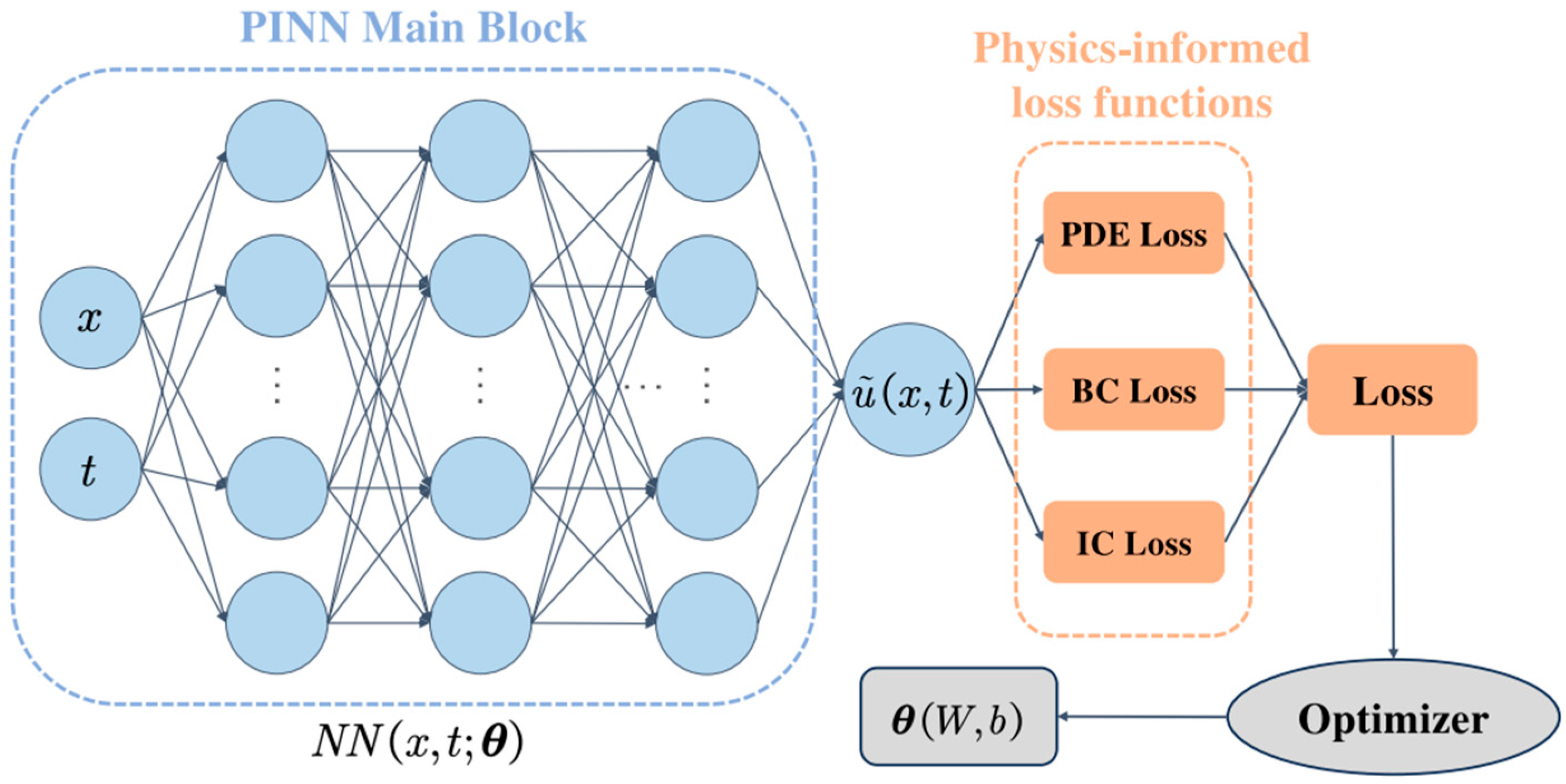
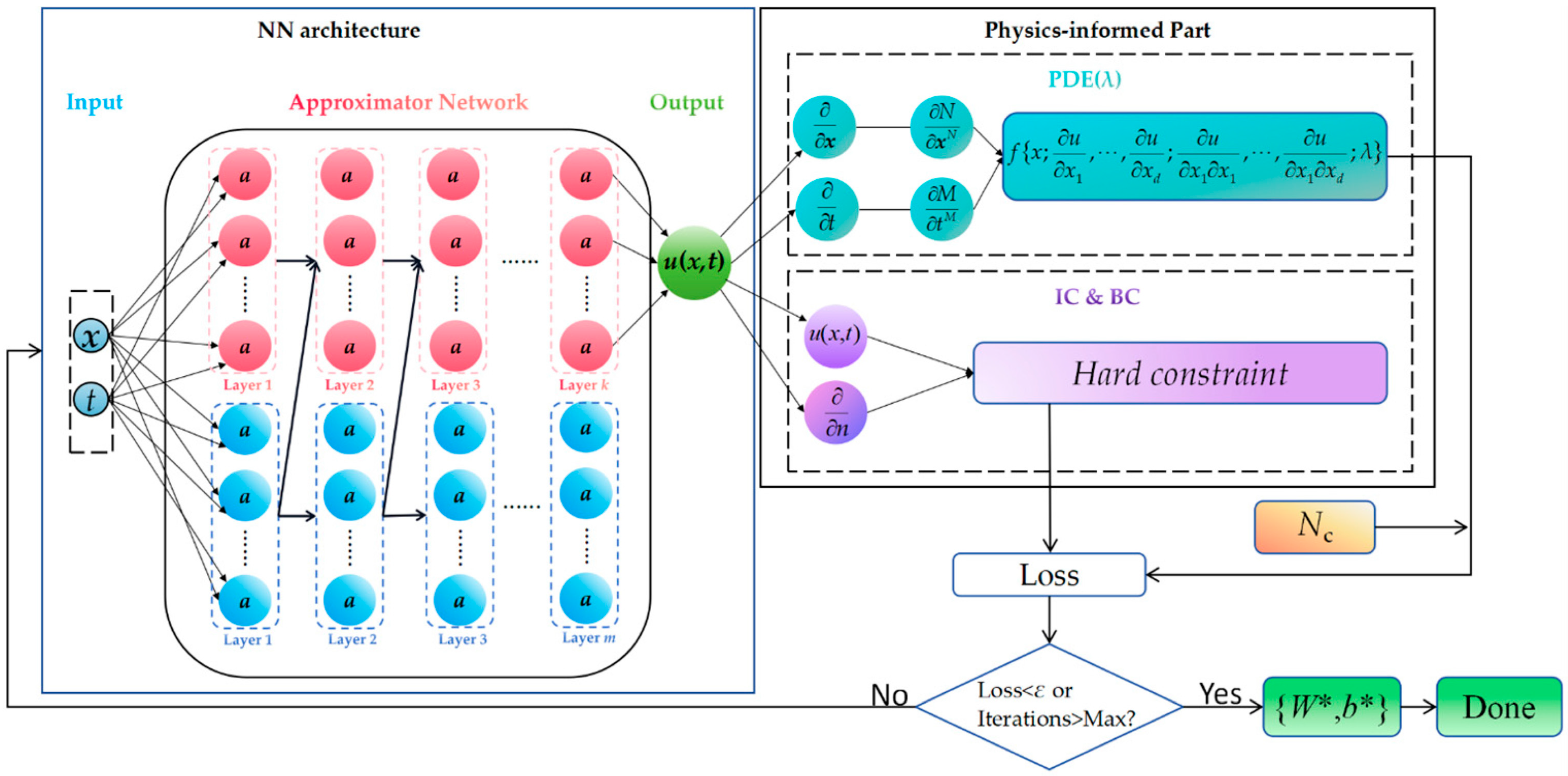
PINNs are deep neural networks used to solve problems described by differential equations. The idea is that the neural network not only approximates the solution but also satisfies physical laws embedded in the form of equations in the loss function (Figure 3).
The approach to PINNs proposed by Raissi et al. in [1] is formulated as follows. For the problem of solving a system of partial differential equations in the form
u t + N u ; λ = 0 ,   x Ω ,   t 0 , T ,
where u ( t ,   x ) is the sought solution; N is the governing differential operator; and λ are equation parameters, with initial and boundary conditions
u ( 0 ,   x ) = u 0 ( x ) ,   u ( t ,   x ) = g ( t ,   x ) on   Ω ,
the neural network u θ t ,   x parameterized by weights θ , approximates the function u ( t ,   x ) . Since the neural network is differentiable, derivatives can be computed automatically and substituted into the following equation:
u f θ t ,   x : =   u t + N u θ ;   λ .
This is the residual of the governing differential equation, which should be approximated to zero for all x     Ω . The total loss function according to Raissi et al. [1] is
L θ = L b + L f ,
where L b is the residual of compliance with boundary/initial conditions
L b = 1 N b i = 1 N b u θ t b i ,   x b i u i 2 ,
L f is the residual of governing equations at internal points of the domain
L f = 1 N f i = 1 N f f θ t f i ,   x f i 2 ,
N b is the number of points with boundary conditions (known values); N f is the number of interior points where PDE error is evaluated.
Although this approach (4)–(6) showed good results, the idea of combining loss components with different physical natures and dimensions seems controversial. This can be mitigated by switching from absolute to relative errors, and for additional regularization, introducing weighting coefficients into the loss function, leading to
L = ω d L d + ω f   L f + ω b   L b ,
where weighting coefficients ω determine the relative importance of each loss term. To select the weighting coefficients in (7), various approaches have been proposed, the main examples of which will be discussed further.

3.1. Methods for Balancing Loss Function Components

The representation of the loss function in the form (7) proved sufficiently effective for simple problems, but, as noted by Krishnapriyan et al. [31], increasing regularization in loss functions makes them more complex to optimize, especially for PDE cases with non-trivial coefficients. The Pareto front analysis for loss function coefficients performed by Rohrhofer et al. [32] showed that multi-objective optimization in PINNs is strongly influenced by the natural form of the Pareto front, determined by the parameters of the governing differential equations and the absolute scale of the studied system. It was noted that the accuracy of the solution for a specific case is usually impossible to determine in advance, and convergence issues remain unresolved.
A logical evolution of the idea of physically reinforced loss functions was the introduction of various algorithms for the adaptive adjustment of weighting coefficients [33]. Liu and Wang [34] proposed assigning weighting coefficients in (7) based on a condition that additionally accounts for the initial conditions error:
ω d   +   ω f   +   ω b + ω i n = 1 ,
ω i = L i L d + L f +   L b + L i n , i d , f , b , i n .
The choice of weighting coefficients according to (8), (9) equalizes the contribution of loss function components at each subsequent training iteration based on error calculations from the previous one.
Further development of the idea of adaptive determination of weighting coefficients in the loss function was proposed in the study by Liu and Wang [35]. Instead of equalizing contributions of loss function components, the authors proposed formulating the PINN training problem as a min-max optimization problem, where weighting coefficients are automatically determined as dual variables that minimize the maximum error among loss function components:
min θ   max α   L θ , α   =   ω i α   L i ,   i d , f , b , i n ,
where weighting coefficients are determined by softmax-type functions
ω i = e x p α i e x p α d + e x p α f +   e x p α b + e x p α i n .
To solve the problem (10), (11) in [35], an algorithm for finding high-order saddle points of non-convex–non-concave loss functions was proposed. On a series of test problems, it was shown that its convergence is significantly faster than the original PINN with an adaptive weighting scheme. To overcome the problem of gradient imbalance in loss function components, Xiang et al. [36] proposed an adaptive approach to balancing them (lbPINN). In this method, weights are dynamically adjusted during training to balance the contribution of each component. Instead of manual weight tuning in the loss function, likelihood maximization based on a Gaussian model is used:
p u x = N u ^ x ; θ , ε 2 ,
where for each component, uncertainty ε i is a training parameter and minimizes the loss function, assuming errors have a normal distribution with zero mean and variance ε i 2
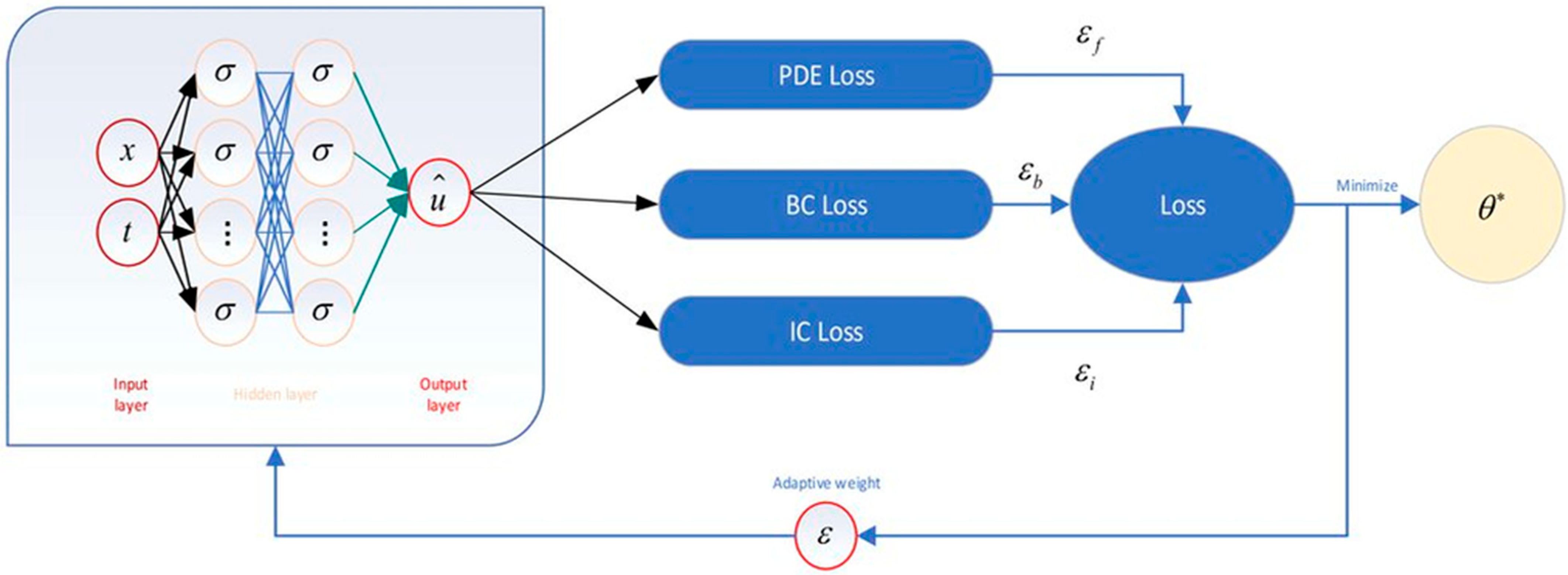
L θ , ε , N = 1 2 ε f 2 L f θ , N f + 1 2 ε b 2 L b θ , N b + 1 2 ε i 2 L i n θ , N i n + 1 2 ε d 2 L d θ , N d + log ε f ε b ε i n ε d ,
where ε = ε f , ε b , ε i , ε d defines adaptive weighting coefficients for each loss function component as ω = 1 / 2 ε 2 .
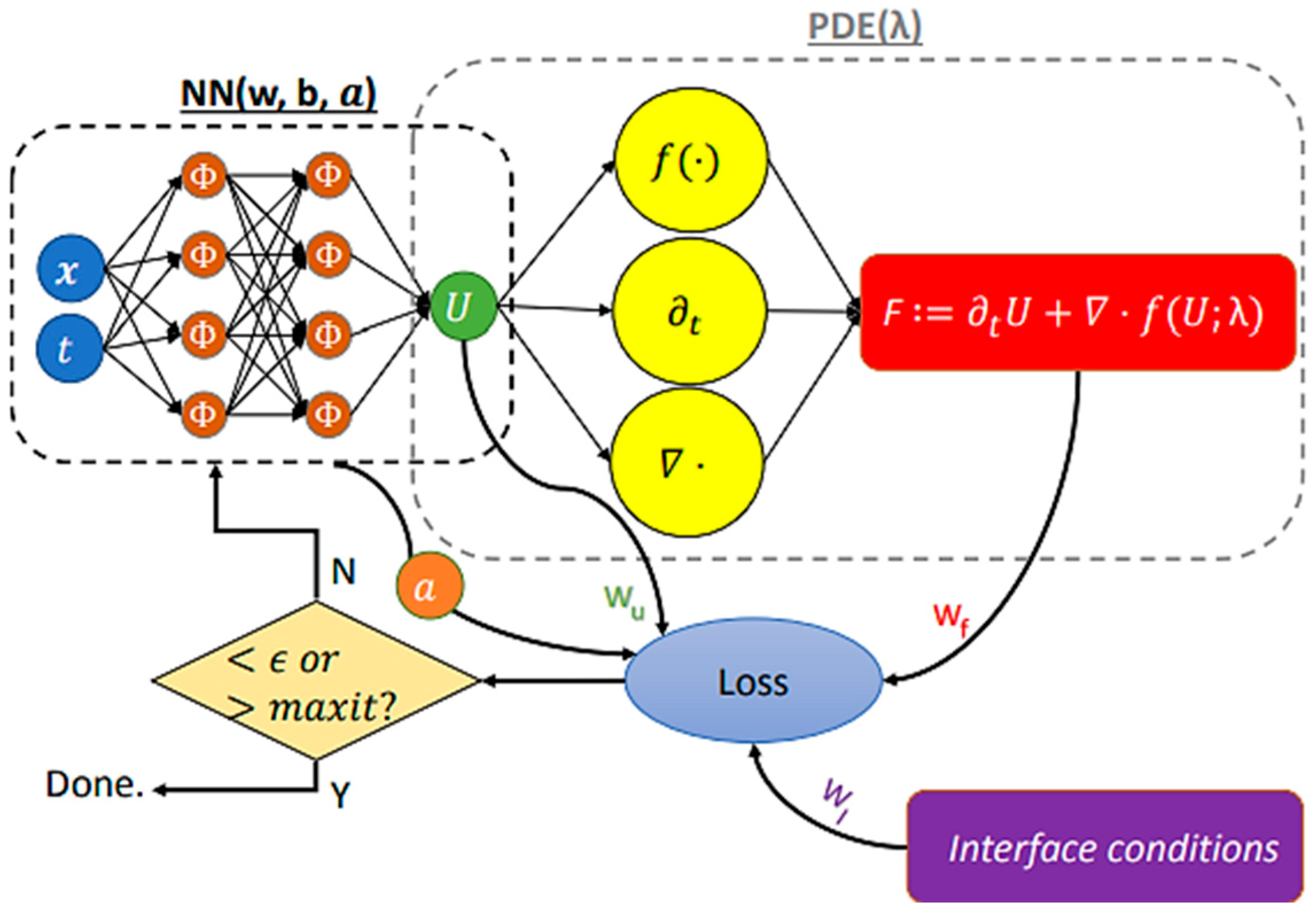
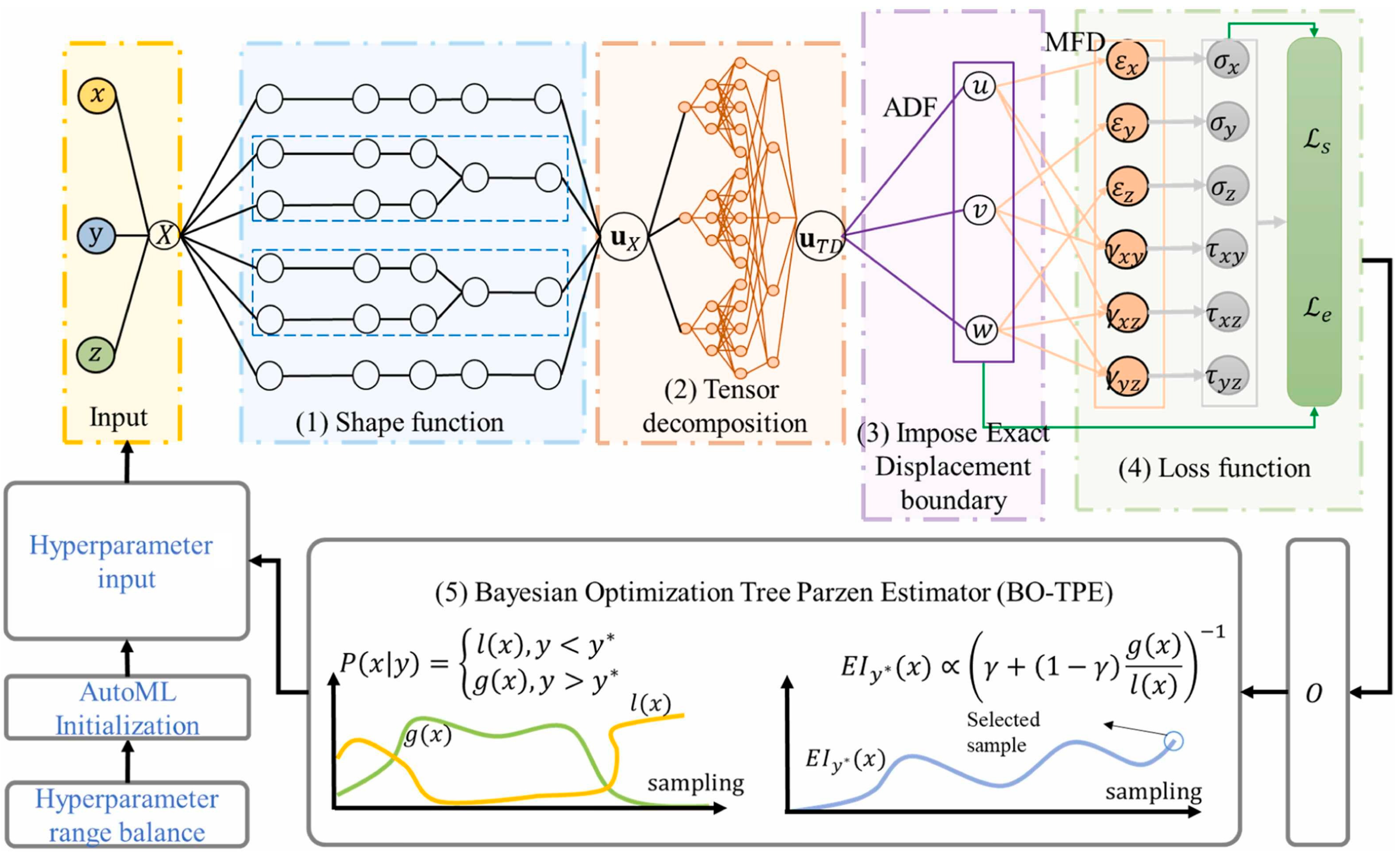
The application of an adaptive approach (12) slightly changes the neural network architecture, which takes the form shown in Figure 4 [37]. Note that the diversity of architecture used in PINNs is detailed in [25,26] and remains beyond the scope of this paper. However, the example in Figure 4 emphasizes that new loss function formulations, changes in geometry accounting methods, and boundary conditions typically necessitate changes in PINN architecture.
The approach proposed by Xiang et al. [36] reduces the risk of domination of the loss function of one component, which is especially important in cases when different physical quantities have different scales. Its advantage is the automation of the balancing process. In subsequent papers, it was demonstrated that this method improves convergence for nonlinear PDEs, such as the Navier–Stokes equations [38]) and in multiphysics problems [37].
Unlike the above approaches, McClenny and Braga-Neto [39] proposed a method for adaptive determination of weighting coefficients in the PINN loss function (SA-PINN), where these coefficients are determined not for the loss function components as a whole, but individually for each training point. Thus, these weights are trainable parameters updated during training along with the neural network weights. The loss function for SA-PINN is written as follows:
L w ,   λ f ,   λ b ,   λ i n = L s w + L f w ,   λ f + L b w ,   λ b + L i n w ,   λ i n ,
where L s ( w ) are losses associated with sensor data (if available); L f w , λ f = 1 / 2 i = 1 N f m λ i f N x , t u x i f , t i f ; w f x i f , t i f 2 is the PDE loss; L b w , λ b = 1 / 2 i = 1 N b m λ i b B x , t u x i b , t i b ; w g x i b , t i b 2 is the boundary condition loss; and L i n w , λ i n = 1 / 2 i = 1 N i n m λ i i n u x i i n , t i i n ; w h x i 0 2 is the initial condition loss.
Here, m ( λ ) is a mask function, which is non-negative, differentiable, and strictly increasing on [ 0 , ) . It transforms weight values λ i into multipliers that amplify or weaken the influence of each point on the loss function. A feature of SA-PINN is that weights λ f , λ b , λ i n are determined simultaneously with network weights w , but with the opposite goal—network weights are updated using gradient descent to minimize the loss function:
w k + 1 = w k η k w L w k ,   λ k f ,   λ k b ,   λ k i n .
Mask weights ( λ f , λ b , λ i n ) are updated using gradient ascent to maximize the loss function with respect to these weights:
λ k + 1 f = λ k f + ρ k f λ f L w k ,   λ k f ,   λ k b ,   λ k i n .
Since weights λ f , λ b , λ i n are tied to specific training points, the basic SA-PINN is incompatible with SGD, where points are resampled. To overcome this, Gaussian process regression (GP) is used to create a continuous weight map in the spatiotemporal domain. The soft attention mask in SA-PINN allows the neural network to adapt to the task by dynamically redistributing attention to problematic points. Thanks to trainable weights and a flexible mask function, SA-PINN achieves high accuracy and efficiency, surpassing traditional PINN methods.
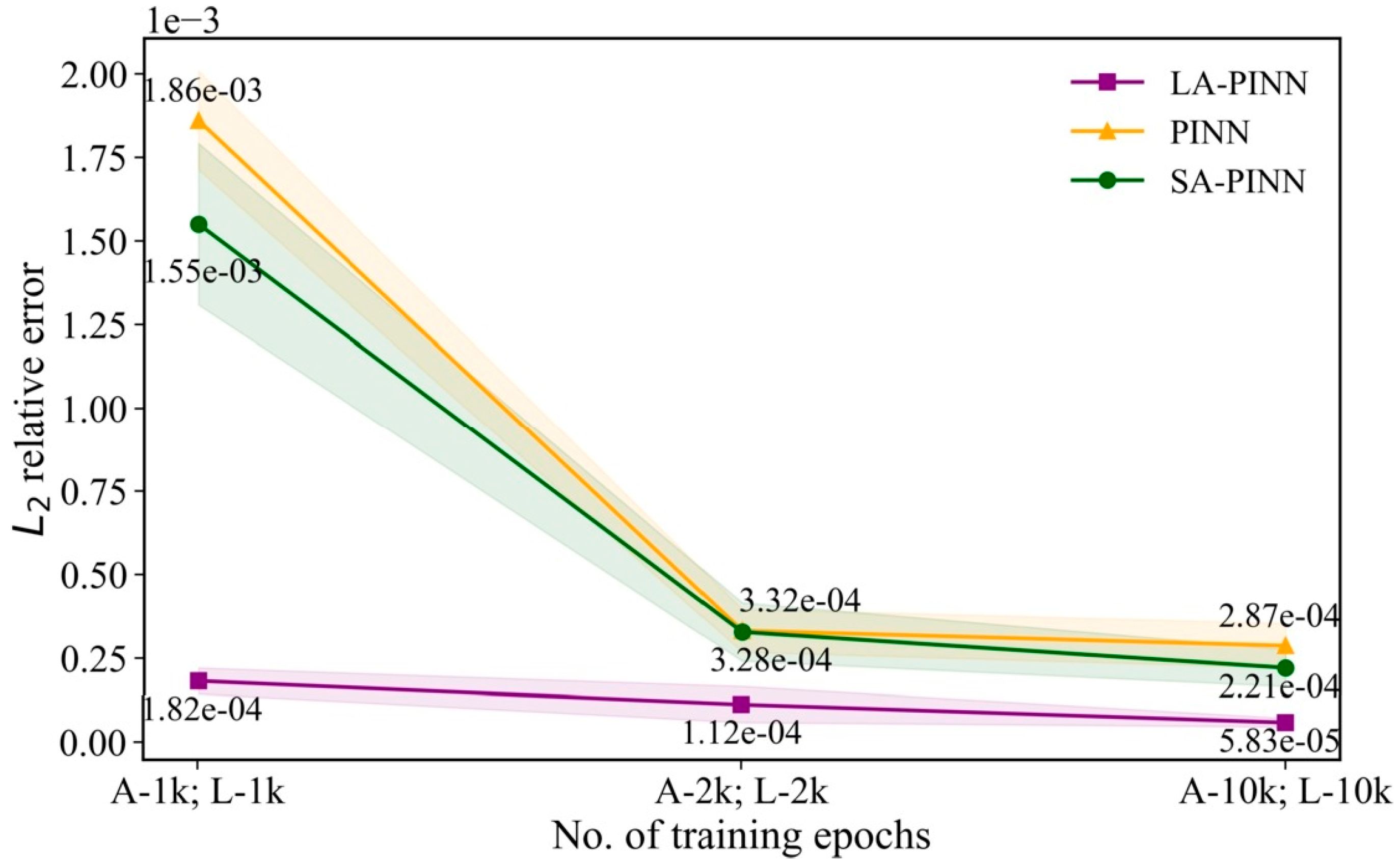
The SA-PINN method was further improved. Zhang et al. [40] used a subnetwork that inputs and outputs the weights themselves to find their values for each point within the residual component. Anagnostopoulos et al. [41] investigated weighting of residual points and proposed a residual-based attention strategy for updating point weights during training. Finally, Song et al. [42] proposed a generalized approach that uses an attention mechanism for dynamic weight distribution between loss components (LA-PINN). This was motivated by the fact that with SA-PINN, minimizing errors for some points is significantly harder than for others. That is, there may be a natural error bias at these points that should be accounted for during training. The model proposed by Song et al. [42] learns not only the weight for the training point error but also includes a bias to account for the overall complexity of error minimization. The distinction is the introduction of independent loss attention networks (LAN) for each loss function component. Unlike SA-PINN, a separate neural network is used to determine weights for errors in the training points in each component. These networks generate weights using an attention function, allowing them to focus on complex points that are dynamically updated during each training epoch. Numerical experiments on several benchmark partial differential equations showed that LA-PINN outperforms both PINN and SA-PINN in predictive accuracy, under identical baseline settings and number of training epochs. The predicted L 2 error is 1–2 orders of magnitude smaller than other methods (Figure 5).
In addition to improving procedures for determining weighting coefficients, efforts continue to improve the loss functions themselves. For data-based loss functions, this primarily involves introducing components containing higher-order derivatives.
Yu et al. [43] proposed a gradient-enhanced PINN (gPINN). The essence of the proposed approach is the assumption that the exact solution of the partial differential equation is sufficiently smooth that the gradient of the PDE residual f ( x ) exists and that, at the exact solution, the PDE residual and its derivatives vanish ( f ( x ) = 0 and f ( x ) = 0 ). The loss function in gPINN is given as follows:
L = w f L f +   w b L b +   w i n L i n +   i = 1 d w g i L g i θ ;   Τ g i ,
where the derivative loss with respect to x i is as follows:
L g i θ ;   T g i =     1 / T g i x T g i f / x i   2 ,
T g i is the set of residual points for the derivative f / x i   .
The effectiveness of gPINN was demonstrated in both forward and inverse test problems [43].
Son et al. [44] developed a similar approach based on Sobolev norms, which includes higher-order derivatives in the loss function to ensure smoothness. This method proved particularly effective for problems with sharp gradients or discontinuities, such as wave phenomena or shock waves, where standard PINNs may yield inaccurate results due to insufficient regularity.
In case of areas of complex shape, their decomposition into simple sub-domains may be applied as in Conservative Physics-Informed Neural Networks (cPINN) [45]. For finding solutions in sub-domains, different neural networks can be used. This makes parallelization of calculations possible, which is quite important from the point of view of achieving computational efficiency. In cPINN the modeling result by neural network for each sub-domain is set as follows:
u i θ x =   N i L x ; θ   ,   i   =   1 ,   2 ,   ,   N s d ,
where N s d is the total number of sub-domains.
The general solution is obtained as follows:
u θ x = i = 1 N s d u i θ x .
The loss function is defined by sub-domains similarly to the base PINN formulation but additionally includes losses on interfaces with corresponding weighting coefficients (Figure 6).
The loss function in this case is written in the form
L i = ω d L d + ω f L f + ω i n t L i n t L i n t = 1 N i n t j = 1 N i n t f p x j , t j · n f p + x j , t j · n 2 + 1 N i n t j = 1 N i n t u p x j , t j { u x j , t j } 2 ,
where u x j , t j = u a v g = : u p + u p + 2 is the average value u on the interface; f p x j , t j · n and f p + x j , t j · n are normal components of flows on the interface, defined by two different neural networks on sub-domains p and p + ; and N i n t is the number of training points on the corresponding interface.
Jagtap and Karniadakis in [46] proposed a more general approach, named eXtended PINNs (XPINNs), which expands the limits of cPINNs. Unlike a cPINN, XPINNs can be extended to any type of PDE. In this case the domain can be decomposed both in space and in time, which is impossible with cPINNs. Thus, XPINNs expand the possibilities of parallelization, thereby effectively reducing the costs of neural network training.
Moseley et al. [47] developed the approach of applying local basis functions for PINNs with finite bases (FBPINN). In FBPINN, neural networks are used for training these basis functions. Numerical experiments have shown that FBPINN is effective at solving both small and large multiscale problems, surpassing standard approaches both in accuracy and in required computational resources.
The problem with the noted approaches is the uncertainty of the principles of decomposition of the computational area into subdomains, although obviously this is the key to their effective application. From this point of view, the use of the progressive domain decomposition method (PDD), proposed by Luo et al. [48], may be promising. The idea of PDD consists of segmentation of the domain based on dynamics of residual losses, with definition of critical sections. Such strategic segmentation allows applying adapted neural networks in defined subdomains, each of which can have different levels of complexity.
During the definition of the loss function, the source of errors can be not only inaccurately balanced components, but also uncertainty of material properties, which are used for computing PDE residuals or boundary conditions. As indicated in many studies, such uncertainty often forms the most substantial contribution to the general model uncertainty (Mangado et al. [49], Sun [50], Berggren et al. [51], etc.). Quantitative estimates show that the error contributed by uncertainty of material properties can reach tens of percent (for example [52]). Considering this, formulation of the loss function in the form (7), (10), (12)–(14) is possible only with accurate definition of material properties, which cannot be ensured in many practical cases of engineering modeling. Proceeding from this, to ensure the accuracy of PINN predictions, it is necessary to account for the uncertainty of material characteristics.
From an analysis of modern research, several strategies for including material properties into PINNs can be distinguished. Firstly, scalar parameters are considered as additional optimization variables. Such a possibility was already considered in the paper by Raissi et al. [1], which served as an impetus for intensive research of PINN applications in inverse problems. Considering the noted problems of uncertainty of material properties, this approach is also used for direct (forward) engineering-modeling problems, e.g., Jo et al. [53], Li et al. [54], etc.
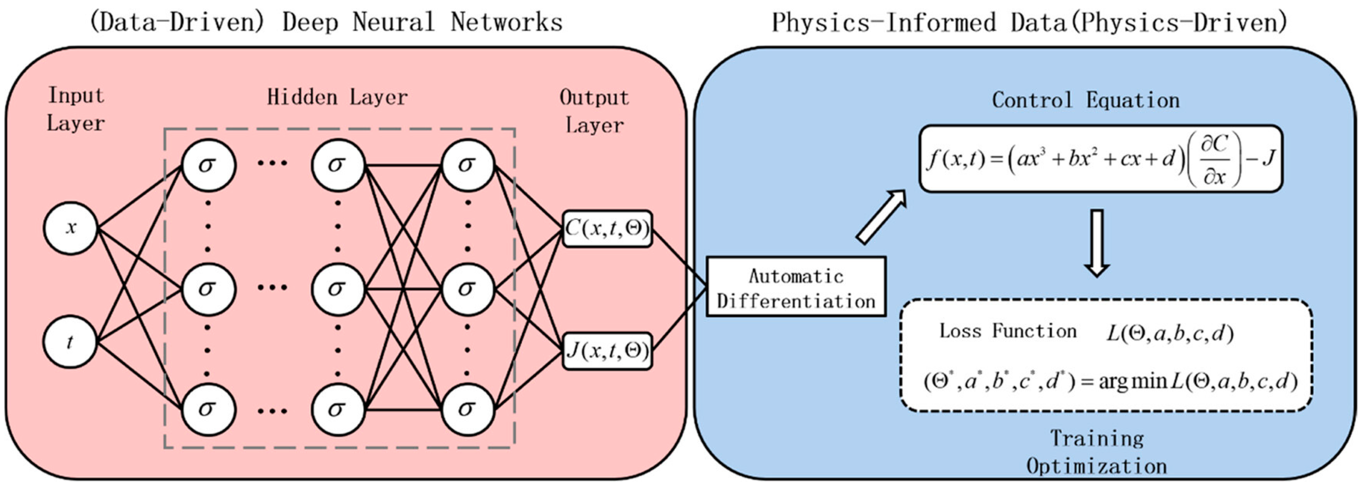
In [53], noisy experimental data were integrated with a wide spectrum of guiding equations and initial and boundary conditions. To solve the problems, the general network architecture was improved for thermal conductivity prediction. In [54] a physics-informed neural network was developed for the problem of diffusion coefficient identification. Sensitivity analysis showed the validity of the model for different combinations of certainty conditions of diffusion flow and concentration gradient. Its architecture was also modified to establish the diffusion coefficient during PINN training (Figure 7). The advantages of such an approach to determining material properties are the simplicity of implementation and faster optimization convergence. It is well suited for tasks with globally constant properties. On the other hand, it is not suitable for spatially or temporally varying parameters and faces the problem of local minima with large numbers of unknown properties.
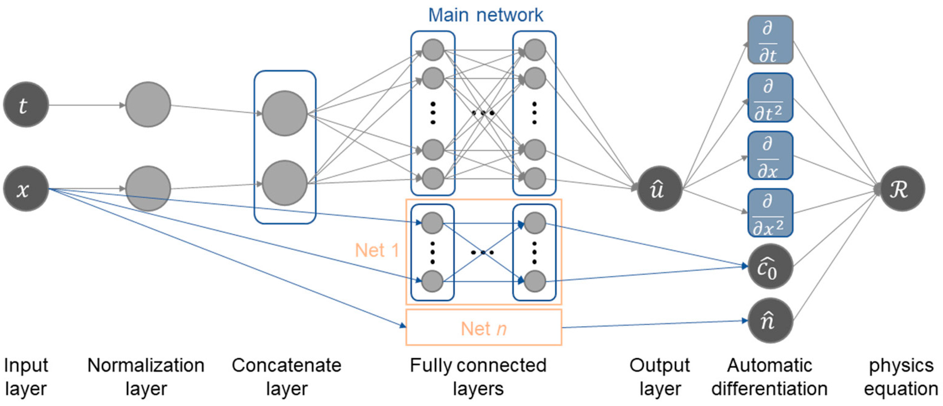
These shortcomings are largely eliminated if uncertain parameters are approximated through separate subnetworks. One of the first publications where such an approach was used was [55], in which two neural networks were used for determining hydraulic conductivity and head. Further studies by Teloli et al. [56] and Kamali et al. [57] confirmed that the use of additional neural networks enables the model to represent spatially and temporally varying parameters, as well as nonlinear constitutive dependencies, which scale better to complex systems.
Figure 8 presents the scheme of a PINN architecture with several additional neural networks, which was applied in [58] for determining the properties of an inhomogeneous material as a spatial function for assessing variations in material integrity and reliability. At the same time, using several neural networks of different types in a single model requires higher computational costs, imposes additional requirements on the amount of data for stable recovery and calibration of characteristics, and is more sensitive to the choice of hyperparameters.
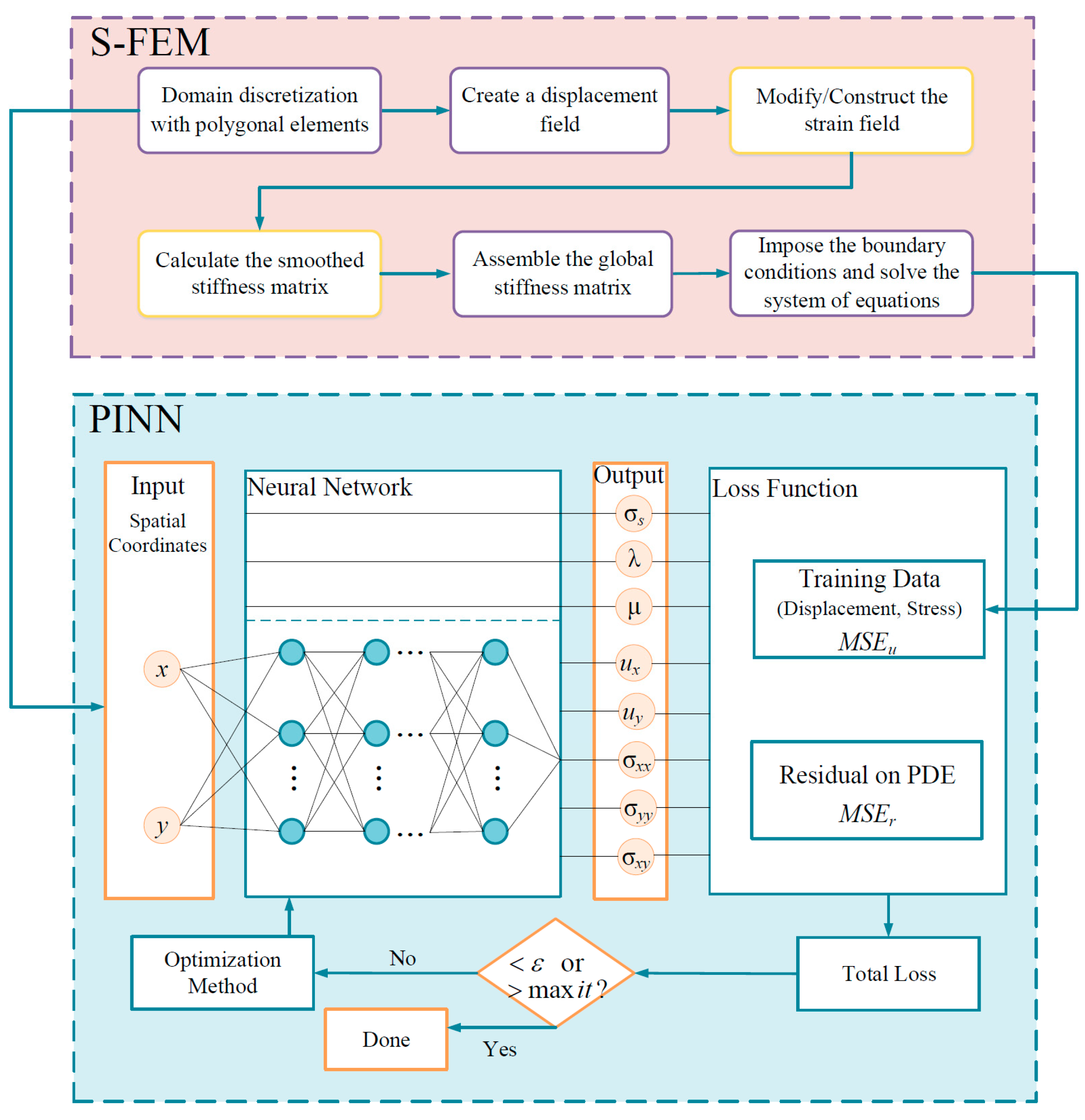
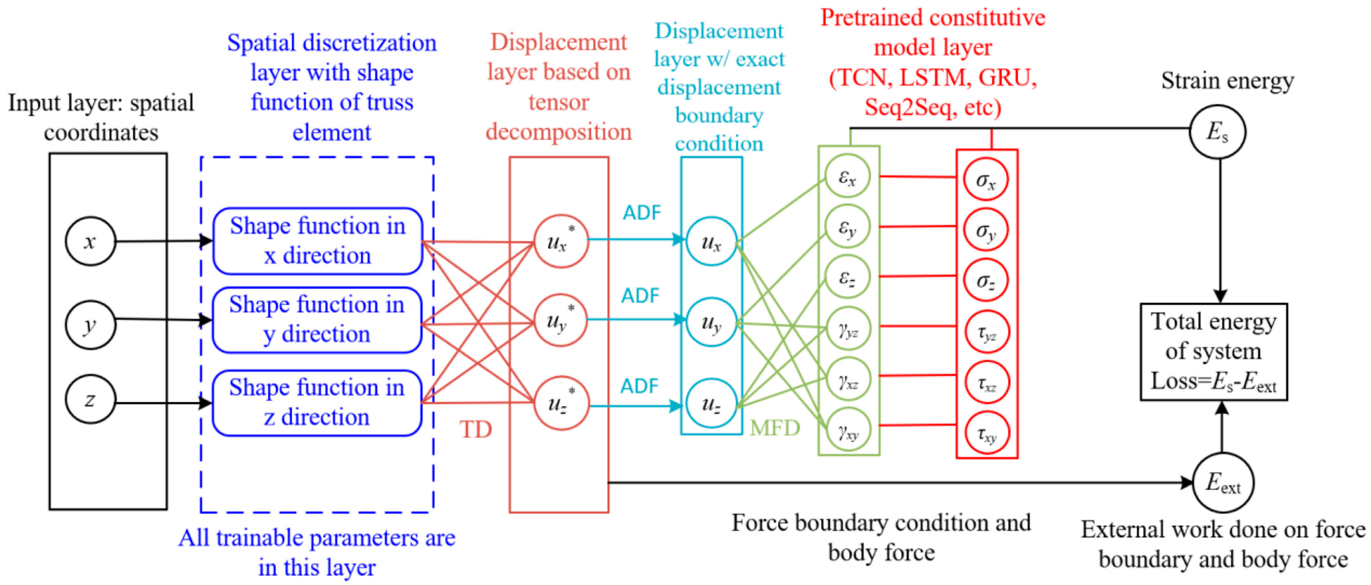
Finally, interest in hybrid approaches is growing, where PINNs are combined with FEMs or ROMs, which provide simultaneous identification of parameters and acceleration of computations. One of the first works where the effectiveness of applying such hybrid models was shown was [59]. Using a series of examples the authors demonstrated the ability to recover missing coefficients and PDE operators from observations obtained directly during the modeling process. Examples of hybrid model applications were given in [60,61]. They considered applications where such hybrid models would allow for identifying parameters, for example, in temperature forecasting and assessment of 3D printing process parameters. In particular, the scheme of the hybrid S-FEM/PINN approach is given (Figure 9).
Hybrid methods show high computational efficiency for direct and inverse tasks; while PINNs integrate physical laws into their neural networks, providing accurate modeling of complex systems, FEM/ROMs reduce computational complexity while preserving accuracy, and inverse PINNs allow the network to determine the material properties (parallel to task solving, using data without manual calibration [62]. Hybrid models adapt to nonlinear and multiphysics problems, which is an undeniable advantage in engineering modeling problems, but combining PINNs with FEM/ROMs requires careful selection of hyperparameters (for example, network architecture, balancing of residuals), which can be labor-intensive and require expertise. Despite the achieved results, even the latest PINN formulations with data-based components and their derivatives do not eliminate the fundamental problem related to the physical interpretation of such methods. Each loss function component in PINNs, such as L f , L b , L i n may correspond to quantities with different physical natures and units of measurement. Direct addition of such quantities in the loss function without proper normalization is physically incorrect.

3.2. Application of Variational and Energy Formulations in PINNs

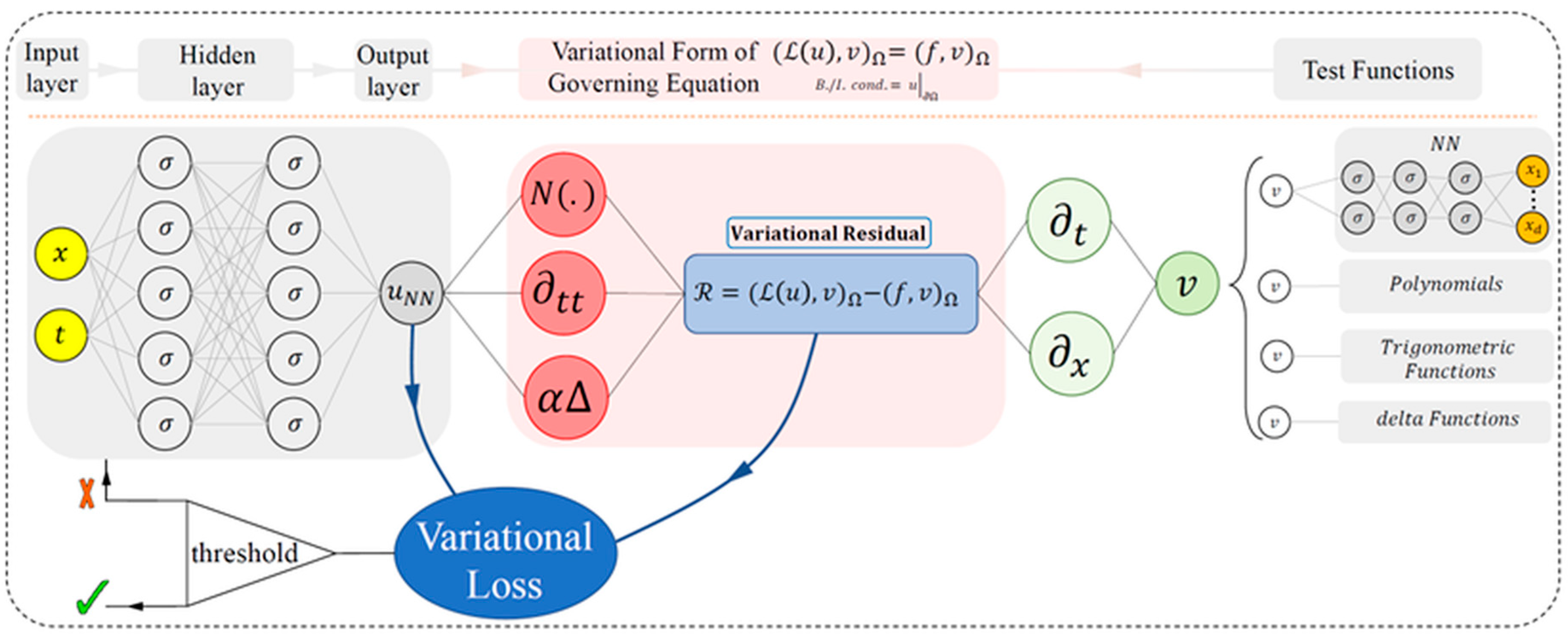
An alternative is writing the loss function based on variational and energy formulations. The main idea of such an approach consists of transition from the direct use of residuals of differential equations (as in standard PINN) to the minimization of energy functionals or use of the weak forms of equations. The main work in which such a possibility was first considered relative to PINNs was the paper by Kharazmi et al. [63], in which the Variational Physics-Informed Neural Networks (VPINN) approach was proposed (Figure 10).
In Figure 10 the red color represents differential operators in the trial space. Green color represents test functions and their derivatives. The blue color represents variational residuals R . The trial functions belong to the neural network space, and test functions can be selected from a separate neural network or other functional spaces, such as polynomials and trigonometric functions. Unlike the classical approach, VPINN uses a weak form based on the Petrov–Galerkin method, leading to an integral component in the following loss function:
L θ   =   1 K i = 1 K Ω φ i x N u θ x f ( x ) d x 2 +   w b   N u j = 1 N u u θ g ( x ) 2 ,
where N [ ] is the differential operator; u θ is the approximation of the solution using a neural network with parameters θ ; f ( x ) is the right-hand side of PDE; φ i x are basis functions; K is the number of basis functions; N u is the number of basis functions; and w b   is the weighting coefficient.
The effectiveness of the proposed approach was demonstrated in several examples, showing clear advantages of VPINNs over PINNs in terms of accuracy and speed. For shallow networks with one hidden layer, Kharazmi et al. [63] analytically obtained various forms of variational residuals, but for deep networks, computing integrals in (15) requires the application of numerical integration, for which additional definition of quadrature rules is necessary. Research in this direction was conducted by Berrone et al. [64,65], who conducted a posteriori-estimates and analysis of convergence for VPINNs, investigated the role of accuracy of numerical quadrature and choice of test-space and analyzed how quadrature rules of different accuracy and piecewise-polynomial basis functions of different degrees influence the convergence rate of VPINNs. According to the data of studies [64,65] it was in particular shown that for smooth solutions the best strategy for achieving high coefficients of error reduction consists of choosing test functions of the lowest polynomial degree in combination with quadrature formulas of high accuracy.
Kharazmi et al. in [63] used globally defined test functions. Other formulations based on variational forms of the problem were developed. In the VarNet variant, proposed by Khodayi-Mehr and Zavlanos [66], test functions were considered piecewise-linear functions of finite element method form, and in the WAN variant [67], an adversarial structure was proposed, where test functions were defined by a separate network. Later Berrone and Pintore [68] proposed using adaptive sets of test functions (Meshfree Variational PINN (MF-VPINN)). For the generation of the test space they used a posteriori error indicator, and test functions were added only where the error was high. Numerical results showed that with this strategy, the solution accuracy was higher than in aVPINN trained with the same number of test functions.
Kharazmi et al. [69] expanded the VPINN idea through the decomposition of the computational domain (hp-VPINN) using the Petrov–Galerkin method with local weighting functions in the form of high-order polynomials, defined on subdomains. Unlike the original VPINN variant, where global polynomials defined on the entire domain were used as test functions [63], in hp-VPINNs each subdomain has its own basis of test functions. This ensures the localization of integrals during the computation of loss functions (integrals in different subdomains are almost non-interconnected), which leads to fewer correlated gradients and more stable training. On a series of test tasks it is confirmed that this allows the network to obtain high accuracy in complex PDEs without the necessity for a global high-order basis, which reduces numerical instability and computational costs. An additional advantage is the ease of implementation through batch-parallelism or multi-GPU.
The mentioned works implement variational approaches to the formulation of loss function based on methods like Petrov–Galerkin (PG), providing a weak form of PDE by integrating the integral from the residual in parts and using different test and trial functions. Greater physical interpretability is ensured by approaches in which, instead of PDE residuals, an energy functional or potential is introduced into the loss function, which means for neural network training, energy minimization is realized. The advantages of this type of method are understandable through physical interpretation: minimal energy corresponds to a stable state of the system. Additionally, the possibility of working with high orders of derivatives without integration by parts is ensured: derivatives from trial functions have already entered the energy functional. It should also be noted that the stability of optimization is ensured by the fact that the energy functional is positive definite, which facilitates gradient-based optimization.
One of the pioneering and most cited works in which an energy approach to formulation of the loss function was applied was the study by Samaniego et al. [70]. The loss function in it is formulated as general potential energy. In the example of solving a number of computational mechanics problem, the advantages of this energy approach compared to the base variant of PINN were shown: better convergence, smaller number of hyperparameters and efficiency for complex geometries without mesh.
In the already-mentioned study by Cuomo et al. [25] a comprehensive review of PINNs is conducted, with focus on energy-based losses as alternative to PDE-residual-based methods. The authors note that loss functions built on energy functionals have fewer hyperparameters and improve generalization for stochastic PDEs and mechanics but may suffer from “null spaces” without data. The article predicts the prospects of applying hybrid approaches with energy-loss for modeling multiphysics tasks, citing [70] as a basis.
In the study by Bai et al. [71], a modified loss function based on Least Squares Weighted Residual (LSWR) is proposed and compared with energy-based and collocation-based losses in PINNs for solid bodies. The energy-based loss showed good stability for linear tasks, but LSWR surpassed it in nonlinear 3D-cases. The authors emphasize that the energy-based approach facilitates the integration of boundary conditions but is sensitive to data scale.
Energy methods are widely applied to forecast the dynamics of systems described by mechanical laws at long time intervals. In these cases, together with PINNs, Lagrangians [72] and Hamiltonians [73] are both widely used. But the most effective use of energy in a PINN may be for related problems [74]. In these cases interaction in different fields is accounted for by integrating all interdependent components into a single energy functional. Instead of computing local residuals (as in residual-based PINNs), the neural network minimizes this single functional, which makes the approach more stable and effective for multiphysics systems.
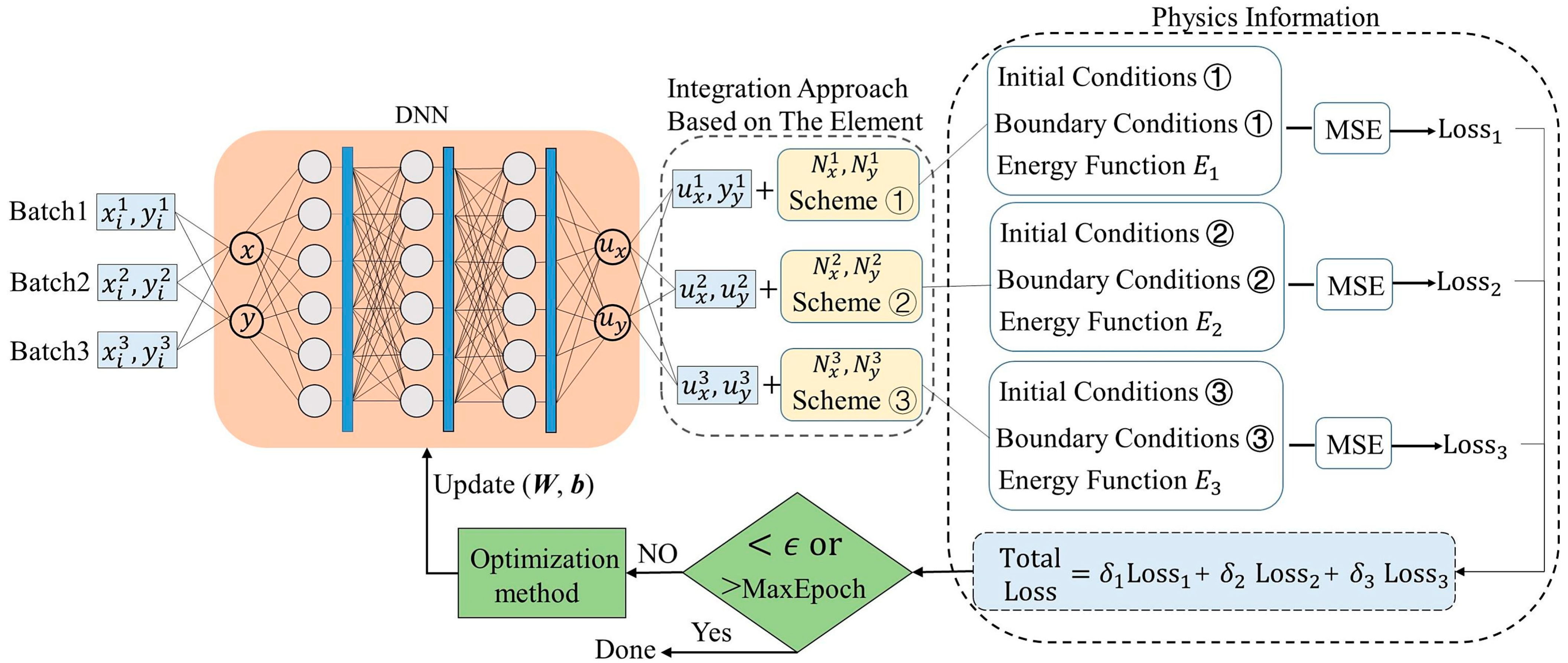
In the study by Liu and Wu [75], the energy approach to formulating the loss function developed from the idea of decomposing the computational domain. The key proposed innovation was calculating equation residuals in subdomains of the computational domain through numerical integration. Test functions and integral weighting coefficients were implemented in the structure of convolutional filters. The approach was demonstrated in problems with a large number of subdomains and showed high parallel processing capabilities. In this aspect, the method surpassed hp-VPINN. Subsequently, Chen et al. [76], instead of global calculation of the energy functional, applied domain division with a calculation of the sum of local energy integrals, determined using quadratures (Figure 11). To improve convergence, it was proposed that a preliminary simplified model be used so as not to start from an “empty” network, but to give it a physically conditioned initial state.
In Table 1, summary information is provided that can be used for preliminary assessment of the efficiency of applying the considered PINN architectures for engineering modeling problems.
Separately, we emphasize the usefulness of including material characteristics, which are components of the physical model of the task, into the composition of neural network training parameters [53,54,55,56,57,58,59,60,61]. This is especially relevant for engineering modeling tasks, where it is necessary to account for uncertainty in structural material properties (Table 2), as well as the environment acting on the modeled structures.
Since multiphysical, including coupled, tasks are quite often encountered in engineering modeling, Table 3 provides a separate comparison of the capabilities of PINNs of different architectures for solving this type of task.
Summarizing the conducted analysis, we note that variational methods use the integral form of PDE, which involves reformulating them into weak formulations and including numerical integration schemes, such as the Petrov–Galerkin or Ritz methods. This requires separate accounting for essential boundary conditions, which are not included in the minimized functional. Applying energy approaches to forming the loss function also requires the correct inclusion of essential and natural boundary conditions either through additional terms or through the requirement of strict compliance with boundary conditions.
Thus, accounting for boundary conditions and geometric information regarding the computational domain are important for the further development of PINN-based methods and require separate consideration.

4. Incorporating Geometry and Boundary Conditions in PINNs

PINNs are a mesh-free method, where the problem geometry (domain Ω and boundary Ω ) is handled through discrete points. Proper handling of geometric information ensures training accuracy, effective incorporation of physical laws (PDE), and boundary conditions (BCs). The sequence of operations with geometric information may vary depending on geometry complexity but generally includes the following steps:
  • definition of domain geometry and boundary: the computational domain Ω is described, and the boundary Ω is divided into parts for different types of boundaries conditions;
  • generation and filtering of collocation points inside the domain and on its boundary, removal from the selection of points that are outside the selection or outside Ω , division of boundary points by types of boundaries conditions;
  • integration of geometry into the loss function, if necessary—construction of functions for strict enforcement of defined types of boundary conditions.
In accordance with this sequence, we will consider the methods used to implement these stages in research related to PINN-based modeling. During the analysis, we will additionally evaluate the possibilities of performing these tasks using tools available in CAD/CAE systems.

4.1. Methods for Incorporating Geometric Information in PINN

The simplest way to determine whether points are located inside the domain or on its boundary can involve various computational geometry algorithms: PIP-type algorithms such as ray casting, winding number [80]), or mesh-based methods [81]. Such methods essentially act as predicate functions, determining whether a point is in the computational domain or outside it. Therefore, in practice, PINN modeling employs analytical methods for incorporating geometric information, which can not only be used in the sampling process but also serve as a tool for constructing the loss function.
The primary such analytical method is the use of Signed Distance Functions (SDF). SDF is defined as the shortest distance from a point x to the domain boundary Ω , with a sign indicating whether the point x lies inside ( φ ( x )   <   0 ) or outside ( ( x )   >   0 ) the domain and equals zero on the boundary. Formally, φ ( x ) =   s g n ( x ) · i n f y Ω x y , where s g n ( x ) is the sign function depending on the point’s location relative to Ω . Prior to the advent of PINNs, SDFs were already a key tool in geometric modeling, robotics, and computer graphics. This was facilitated by the convenience of describing complex bodies and surfaces, as well as mesh independence. From the SDF definition follows the equality for its ideal (differentiable everywhere) form—the Eikonal equation:
φ x = 1     x R n \ Ω ; ,   φ | Ω = 0 .
Numerical methods (Fast Marching, Fast Sweeping, etc.) form the core of classical approaches to computing SDF. An overview of the corresponding concepts is systematized in the papers by Sethian [82,83]. Based on this, several methods have been developed for constructing SDF for domains of complex shapes, differing in accuracy, computational costs, and frequency of usage.
The most popular among them is the analytical method using geometric primitives. It is applied when the form of the computational domain can be created by applying Boolean operations to geometrically simple objects for which SDF exists in analytical form. Such functions are used as building blocks for the SDF of the entire domain using operations such as union φ ( x )   =   m i n φ A x ,   φ B x , intersection φ ( x )   =   m a x φ A x ,   φ B x , and difference φ \ ( x )   =   m a x φ A x ,   φ B x (e.g., [84]). The method surpasses all others in simplicity, computational costs, accuracy, and frequency of use. The drawback is the limitation to applications where the domain can be constructed from regions with available analytical SDF. Additionally, the m i n and m a x functions are not smooth on lines/hypersurfaces where the arguments φ A x ,   φ B x are equal. To overcome this limitation in PINN modeling, either smooth approximations like s o f t m i n or s o f t m a x can be used, or a transition to subgradients can be made [85].
One of the classical methods is a direct distance computation from triangular meshes, where the unsigned distance to each triangle is obtained by projection onto the plane while accounting for regions near vertices, edges, and faces, and the sign is determined using surface normals or angle-weighted pseudonormals, N   =   ( i n i θ i ) / | | i n i θ i | | , where n i are face normals and θ i are the angles. This approach, detailed in the survey by Jones et al. [86], emphasizes accuracy and efficiency thanks to hierarchical structures such as octrees, which reduce the complexity from O ( M ) to O ( l o g   M ) for M triangles. The method integrates well with modern CAD systems because all of them are compatible with the STL format. STL represents an object’s surface as a set of triangles specified by their vertex coordinates which are, typically, face normal—i.e., everything needed to construct an SDF using this method [87]. Several libraries, such as Open3D or libigl, allow direct STL import and SDF computation for PINNs or other applications. For complex geometries with an excessive number of facets, mesh simplification may be required to reduce the computational cost of the SDF. The method is characterized by high accuracy and, for these reasons, is widely used, but it entails substantial computational expense.
SDF can be found as the solution to the boundary value problem for the Eikonal equation | φ | = 1 with boundary condition φ Ω = 0 . In practice, this equation is solved numerically on a grid using ordered methods: Fast Marching (FMM)—a one-pass algorithm similar to Dijkstra for continuous distances; Fast Sweeping—an iterative method using passes in multiple directions and effective for regular grids. Both classical approaches have well-developed theory and are applied in many CAD/CAE systems [82,83]. Fayolle [84] proposed a method for redefining the distance to an implicit surface. For function f , whose zero level defines the geometric surface S , SDF was determined by embedding f in the last layer of a deep neural network trained on a loss function derived from the Eikonal equation. These methods are applied less frequently, have accuracy issues in high-curvature zones, and require moderate computational resources.
Neural methods, such as DeepSDF, represent SDFs as continuous functions trained on point samples, where the neural network f θ ( x ) is optimized using the loss function L ( f θ ( x ) ,   s )   =   | c l a m p ( f θ ( x ) ,   δ )     c l a m p ( s ,   δ ) | , where c l a m p ( z ,   δ )   =   m a x ( δ ,   m i n ( δ ,   z ) ) which limits z values within [ δ ,   δ ] , s is the true SDF value, and f θ ( x ) is the predicted value, enabling interpolation and form completion for object classes. Park et al. [88] demonstrate this method’s advantage in compression and reconstruction quality over mesh representations, although training requires large datasets and may suffer from overfitting to specific shapes.
One of the limitations of neural approaches is the need for ground-truth signed values or directed surface normals. To address this, Sign-Agnostic Learning (SAL, [89]) emerged, allowing implicit representation training even from “unsigned” data (e.g., simple point clouds), and Neural-Pull [90], which trains the network to “pull” space points to the surface using predicted distances and gradients as steps for query point movement. These approaches significantly expand the dataset for direct training of SDF-parametric models and enable the training of differentiable SDFs without explicit signed labels. Neural network-based methods require very high computational costs during training but operate extremely fast afterward, providing the highest accuracy for complex geometric forms.
Sukumar and Srivastava [91] explored the use of another method in PINN modeling that accounts for computational domain geometry at the analytical level—the R-functions method. The idea of this approach is to use functions that are algebraic but have properties of logical algebra functions in the sense that their sign is fully determined by the sign of their arguments. Such functions ( R -functions) were first proposed by Rvachev [92] for use in solving PDE problems with variational methods. An R -function is a real-valued function Φ u 1 , u 2 , , u n that has the same sign structure as some Boolean function B ξ 1 , ξ 2 , , ξ n , ξ i 1 , + 1 . That is, if the Boolean function B is true for a certain set of signs u i , then Φ > 0 ; if false—then Φ < 0 . Using R -functions, analytical functions describing domains of arbitrary geometric shapes can be constructed. For example, for two domains described as Ω 1 : f 1 ( x , y ) 0 , Ω 2 : f 2 ( x , y ) 0 , with a complete system of R -functions can be defined as follows [93]:
intersection   Ω 1 Ω 2   as   R f 1 , f 2 = f 1 + f 2 f 1 2 + f 2 2 , union   Ω 1 Ω 2   as   R f 1 , f 2 = f 1 + f 2 + f 1 2 + f 2 2 , omplement   Ω ¯ 1   as   R ¬ f 1 = f 1 .
Thus, having a set of geometric primitives f i : R n R i = 1 , , k with domains Ω i = { x : f i ( x ) 0 } and a Boolean formula B : 1 , + 1 k { 1 , + 1 } describing the target domain Ω through operations , , ¬ over Ω i , using R -function Φ B : R n R , a function φ ( x ) = Φ B ( f 1 ( x ) , , f k ( x ) ) with which properties can be constructed:
x R n :   φ x > 0 x i n t   Ω ,           φ x = 0 x Ω ,                   φ x < 0 x R n \ Ω ¯ .
The function φ x = 0 , constructed from geometric primitives in implicit form using system (17) or its analogs, is analytical everywhere in Ω , except on curves/surfaces where the arguments are equal to f 1   =   f 2   =   0 , where the derivatives are bounded but vary depending on the direction. In addition to (17), other complete sets of R-functions exist that can be applied for the analytical description of regions with complex shapes [92,94], which possess different properties of smoothness and differentiability:
R 2 f 1 , f 2 = f 1 · f 2 / f 1 2 + f 2 2 R 2 f 1 , f 2 = f 1 · f 2 / f 1 2 + f 2 2 ,
  • C 1 -continuous (first derivative exists) but not smooth in sign-change zones;
R α f 1 , f 2 = 1 / 1 + α · f 1 + f 2 f 1 2 + f 2 2 2 α f 1 f 2 R α f 1 , f 2 = 1 / 1 + α · f 1 + f 2 + f 1 2 + f 2 2 2 α f 1 f 2 ,
  • for 0 < α < 1 is smooth almost everywhere, approximates the distance function without singularities; parameter α controls the “thickness” of medial zones;
R m f 1 , f 2 = f 1 2 + f 2 2 m / 2 · f 1 + f 2 f 1 2 + f 2 2 R m f 1 , f 2 = f 1 2 + f 2 2 m / 2 · f 1 + f 2 + f 1 2 + f 2 2 ,
  • m-times differentiable everywhere with vanishing derivatives in singularities.
The systems of functions (17), (19)–(21) are not only used for describing the geometry of the computational domain in the form (18). The main idea of the R-functions method lies in the possibility of creating bundles of functions with uses that identically satisfy arbitrary boundary conditions in PDE problems, termed by Rvachev [92] as solution structures. To this end, the concept of a function φ ( x ) normalized to order k , is introduced. According to [92], such a function has additional properties:
m φ x n m = δ m 1 ,   x Ω ,   m = 1,2 , , k ,
where / n denotes the derivative in the direction of the outward normal to the boundary, and δ m 1 is the Kronecker symbol (equals 1 for m = 1 and 0 for m 1 ).
In [92], it is shown that if φ x C m R n R satisfies conditions φ x Ω = 0 , φ x / n Ω > 0 , then a first-order normalized function can be constructed as follows:
φ 1 x φ φ 2 + g r a d   φ 2 1 / 2 C m 1 R n .
Constructing normalized functions using expression (23) may require additional computational costs, but these can be eliminated if normalized equations for geometric primitives are used for constructing complex geometry. Operations (17), (19)–(21) over them preserve the normalization of the result. For geometric primitives, normalized functions in implicit form can be constructed by simple multiplication by some constant.
In addition, note that if Ω = φ = 0 = 0 is a first-order normalized equation of the boundary Ω , and Σ = ( σ 0 ) is some region, then
φ 1 φ 2 σ ¯ = 0 ,
where is one of the R-disjunctions from systems (17), (19)–(21) and is a first-order normalized equation of the element Ω 1 = Ω Σ [92].
Sukumar and Srivastava in [91] applied such an approach to define approximate distance functions (ADF) for boundary segments. Using SDF as the base and a first-order normalized equation of the corresponding region as the trimming function, they obtained functions that satisfied conditions φ i ( x ) = 0 x Ω i , and approximately defined the distance to Ω (Figure 12).
Finally, if φ 1 = 0 , φ 1 C m Ω Ω is a first-order normalized equation of Ω , then normalized equations of higher orders Ω are determined by recursive relations:
                  φ 2 x = φ 1 1 2 ! φ 1 2 D 2 φ 1             φ n x = φ n 1 1 n ! φ 1 n D n φ n 1 ,
where D n · = α = m m ! α ! i = 1 n φ x i α i n · x 1 α 1 x n α n is the operator of continuation inside the region Ω of the operation of n-fold differentiation along the normal to Ω [92].
An alternative approach to analytically describing complex geometries in PINNs involves the use of phi-functions, originally developed by Stoyan for geometric modeling and object placement problems [95], and further elaborated in numerous studies (e.g., [96,97,98,99,100,101,102]). Unlike SDFs, which encode the distance from a point to the boundary, phi-functions describe the relative positions of two objects through a functional dependent on their parameters, such as distances between surfaces or the degree of overlap. Phi-functions analytically represent placement constraints, including non-overlap, containment, prohibited zones, and allowable distances, for arbitrarily shaped objects that may be connected or disconnected, convex or non-convex, may include holes, cavities, and admit special transformations (e.g., translations/rotations, scaling, stretching/deformation).
For the readers’ convenience, basic definitions of different types of phi-functions are provided below. Let us consider two geometric objects A R d and B R d ( d = 2,3 ) . The position of A ( B ) is defined by a variable motion vector u A ( u B ). Phi-functions allow us to distinguish the following three cases: A and B are intersecting, i.e., A and B have common interior points; A and B are in contact, i. e. A and B have only common boundary points; A and B do not intersect, i. e. A and B do not have common points.
Definition 1 
([96]). A continuous and everywhere-defined function phi-function ΦAB(uA, uB) that meets the following properties:
Φ A B < 0   for   int A int B ,
Φ A B = 0   for   int A int B = and   f r A f r B ,
Φ A B > 0   for   A B = ,
where int(.), int(.) denote the topological interior and boundary of geometric object (.).
The inequality Φ A B ( u A , u B ) 0 holds the non-overlapping condition, i.e., int A int B = , while inequality Φ A B * ( u A , u B ) 0 ensures the containment condition A B , i.e., int A int B * = , where B * = R d \ int B .
While the sign of the phi-function plays a crucial role, its absolute value is not subject to any rigid requirements. If two objects A and B overlap, then Φ ( u A , u B ) < 0 and the absolute value | Φ ( u A , u B ) | can just roughly define the extent of overlap. For non-overlapping objects Φ ( u A , u B ) > 0 , and the value of Φ ( u A , u B ) may just roughly correspond to the distance between A and B .
When objects do not overlap, one can set Φ ( u A , u B ) = d i s t ( A , B ) , where
d i s t A , B = min X A , Y B d i s t ( X , Y ) ,
denotes the Euclidean distance between two phi-objects.
Let minimal allowable distance ρ > 0 between objects be given.
Definition 2 
([96]). A phi-function   Φ ~ A B ( u A , u B )   is called the normalized phi-function for objects A and B if the values of the function coincide with the Euclidean distance between objects A and B when   int A int B = .
The inequality Φ ~ A B ( u A , u B ) ρ provides the distance condition for objects A and B .
In many cases the formula for the distance involves radicals, which makes it difficult for local optimization algorithms to use phi-function and its derivatives. In those cases, phi-function should be defined by a simpler formula which holds the allowable distance between the objects. However, if distance conditions must be considered, other forms of phi-functions are needed, because the values of the phi-functions above do not coincide with the Euclidean distances between the corresponding shapes when they do not overlap. To simplify the distance constraints an adjusted phi-function can be applied.
Definition 3 
([96]). A continuous and everywhere-defined function   Φ A B ( u A , u B )   based on variables   u A , u B   is called an adjusted phi-function for objects A and B if
Φ A B > 0   for   d i s t ( A , B ) > ρ ,
Φ A B = 0   for   d i s t ( A , B ) = ρ ,
Φ A B < 0   for   int A int B < ρ .
The inequality Φ A B ( u A , u B ) 0 ensures the distance condition, i.e., d i s t ( A , B ) ρ , while inequality Φ A B * ( u A , u B ) 0 provides the distance condition d i s t ( A , B * ) ρ , i.e., where B * = R d \ int B .
For some shapes under motion, an alternative to phi-functions, the use of quasi phi-functions, allows us to simplify descriptions of non-overlapping constraints at the expense of a larger number of variables.
Definition 4 
([96]). A continuous and everywhere-defined function   Φ A B ( u A , u B , u )   is called a quasi-phi-function for objects   A ( u A )   and   B ( u B )   if   m a x u R n Φ A B ( u A , u B , u )   is a phi-function for these objects.
The non-overlapping constraint for objects A and B can be described as follows: if Φ A B ( u A , u B , u ) 0 for some u , then int A int B = .
Definition 5 
([96]). A continuous and everywhere-defined function   Φ ~ A B ( u A , u B , u )   is called a normalized quasi-phi-function for objects   A ( u A )   and   B ( u B )   if   m a x u R n Φ ~ A B ( u A , u B , u )   is a normalized phi-function for these objects.
The phi-function technique is a versatile tool for describing placement problems as mathematical programming models. It leverages nonlinear programming (NLP) for open dimension problems and mixed-integer nonlinear programming (MINLP) for knapsack problems, representing the solution space as a union of subregions defined by smooth inequalities derived from the phi-function expressions. Constructed using min-max operators, phi-functions are continuous and piecewise smooth, which enables efficient modeling of placement problems while supporting fast, feasible solutions through smart heuristics. The phi-function technique is widely applied to solve different classes of practical problems that arise in nanotechnologies, materials science, aerospace engineering and additive manufacturing [103,104,105,106,107,108].
In the context of PINNs, phi-functions offer flexible representations for complex multi-body geometries because they naturally encode intersection and non-intersection relations. In practice, they can enter the learning objective either as penalization terms that discourage interpenetration and boundary violations or as analytical building blocks for hard-constraint ansätze. However, standard phi-functions are continuous but only piecewise smooth (built via min/max), and they do not provide a local metric like SDF (i.e., no direct distance-based normals), which complicates gradient-based training for tasks requiring Neumann data. This is why a hybrid strategy is recommended: use phi-functions for global placement constraints and SDF for accurate local boundary enforcement and normals. From a learning perspective, this role of phi-based geometric penalties is analogous to recent reinforcement-learning setups for packing, where dense rewards directly encode minimum-distance and non-overlap constraints; see Yamada et al. [109] for an example with PPO agents optimizing the maximum pairwise/boundary distance ρ and explicitly comparing against a phi-function-based baseline.
A hybrid approach combining phi-functions for global geometric constraints with SDF for precise local boundary specification is most promising. This strategy leverages phi-functions’ strengths in handling complex multi-body configurations and optimization tasks while using SDF to ensure accurate boundary condition enforcement.
For instance, in optimization-driven PINN applications, such as shape optimization, phi-functions can serve as a natural functional to enforce global placement constraints while SDF ensures local geometric accuracy. The comparison between SDF and phi-functions in the context of PINNs is summarized in Table 4.
In addition to the theory of R-functions, Sukumar and Srivastava in [91] considered another approach to constructing approximate distance fields based on the theory of mean value potential fields and related to transfinite barycentric coordinates (TFC) [110]. TFC are constructed through harmonic functions or other generalized interpolation schemes that preserve the properties of classical coordinates, and the computational domain is defined through these coordinates as an analytical combination of local primitives. TFC are defined as analytically smooth functions throughout the domain, which practically eliminate the risk of “gradient explosion”. At the same time, TFC can only be applied to regions that can be described by a polygon/polyhedron, limiting their usage possibilities. Information regarding the advantages and disadvantages of the methods described for incorporating geometric information is summarized in Table 5.
Considering the features of the approaches described, let us examine the next stage of integrating geometric information into PINN algorithms—the generation of the training point sample.

4.2. Sampling of Collocation Point for Physics-Informed Neural Networks

First, note that the application of neural networks for engineering modeling may be most interesting as a means of radically reducing the time to obtain results [75]. Therefore, practically all leading companies in CAE software are intensively working on implementing neural network technologies in their commercial packages—ANSYS, Autodesk, Siemens, Dassault Systèmes, etc. [111].
Such an application assumes that, either as an add-on to the package or as a user library, a training database for PINNs will be formed for a certain class of problems, allowing sufficiently accurate predictions even for geometric forms not included in the training data. The presence of such an initial approximation allows users to obtain solutions in the shortest time using PINNs.
To form such datasets, it is necessary first to normalize geometric information so that coordinates for all examples are in the range [ 0 , 1 ] or [ 1 , 1 ] . This is usually performed in several steps: forming a sample of training points x i , y i , z i ; finding the bounding box x m i n , x m a x , y m i n , y m a x , z m i n , z m a x ; finding the center c x = x m a x + x m i n 2 ; shifting the coordinate origin to the determined center; determining the scale s = max x m a x x m i n , y m a x y m i n , z m a x z m i n ; and normalization, for example, to [ 1,1 ] x = 2 x / s . Determining the center based on the m i n m a x bounding box approach is dominant in modern research, e.g., Anton et al. [112,113], Valente et al. [114].
The selection of training points is one of the most important stages in building a PINN-based model. The study by Wu et al. [115] is one of the few papers where this issue is systematically covered. The authors considered ten methods for generating training point samples, including six non-adaptive and four adaptive. Among the non-adaptive uniform sampling methods, uniform grid, uniform random sampling, Latin hypercube sampling, Halton sequence, Hammersley sequence, and Sobol sequence were considered (Figure 13).
In most studies performed using PINNs, training points are determined at the very beginning and do not change thereafter. This choice is driven by simplicity of implementation, stability, and predictability of computational costs. Uniform discretization ensures coverage of the entire domain, even in areas with initially small residuals, preventing local overfitting that may occur with adaptive concentration of points in high-residual zones. From the perspective of integration with existing CAE packages, mesh-oriented methods have certain advantages. They allow direct use of existing CAD geometries and mesh and ensure concentration of points in important areas, as the mesh generator already adapts element density to these needs.
Nevertheless, adaptive methods, characterized by dynamic reconstruction of the training point sample, are becoming increasingly popular, as they allow faster reduction in residuals precisely where it most affects solution accuracy and usually lead to faster model convergence (by orders of magnitude for problems considered by Wu et al. [115]) with significantly fewer total training points. This is particularly relevant for problems in domains of complex shapes, with steep gradients and multiscale behavior [116].
The number of studies on improving adaptive generation of training point samples is rapidly growing. Classifying adaptive methods by used metrics, the most used in current research is adaptive distribution based on PDE residuals, where the magnitude f θ t f i , x f i at a point is considered an indicator of local model inaccuracy, and points with the largest residuals receive higher priority in regeneration [115,117]. A more advanced approach is DAS-PINNs [118], where the PDE residual is viewed as a probability density function and approximated using a deep generative model. New samples are aligned with the distribution induced by the residual, i.e., more samples are placed in high-residual areas and fewer in low-residual areas.
Lin and Chen [119] extended the residual-based approach to unsteady problems, proposing a causality-driven method. Collocation points selected at each step are released before the next sampling step to avoid cumulative effects and reduce computational costs. The criterion for selecting collocation points at time steps is the largest weighted residual ω p L f t i , x , θ , where p 0 is a hyperparameter and
L f ( t , x , θ ) = u θ t t , x + N u θ t , x 2 .
For updating p from an initial value p 0 , Lin and Chen in [119] proposed a time-aligned update scheme (TADU):
p n + 1   =   p n β 1 tanh β 2 t a d a t ω 1 + 1 ,   n   =   0 ,   1 ,   ,
where parameter β 1 0 , 1 regulates the maximum variation coefficient for p , and β 2 > 0 controls the difficulty level of achieving the maximum variation coefficient, and t a d a indicates the time when the previous batch of adaptive collocation points is concentrated, t ω for k 0.5 , 1 ) is determined by the model training time as follows:
t ω = m i n t i : ω i < k ,   ω N t < k , T 1                                                   ,   ω N t k .
The second most used method for creating training point samples in PINNs is using the PDE residual gradient ( f θ t f i , x f i ) . In practice, three working patterns have formed: gradient-driven algorithms—build a probabilistic distribution proportional to f θ t f i , x f i α , then shift or regenerate collocation points [115,120]; hybrids with PDE residuals, using weighted combinations of f θ t f i , x f i and ( f θ t f i , x f i ) [121] or two-stage sorting [117] to avoid oversaturation of points in areas where the gradient is large but the error is small; anisotropic strategies—orient local “clouds” of new points along the direction of maximum residual growth (using directional derivatives) to better capture thin layers [122,123]. Advantages of gradient-oriented approaches include faster detection of boundary layers, shock waves, and thin structures; better accuracy/sample balance for a fixed number of points; and fewer “blind spots” compared to purely residual methods. However, such approaches have higher computational costs (need to differentiate residuals by inputs, sometimes repeatedly), noisiness and instability of residual gradient estimates at early stages, risk of local overfitting, and loss of global coverage.
Other methods for adaptive generation of training points for PINNs are less commonly used. Among them, those using loss function residuals or energy functionals as metrics [124] can be highlighted. Also noteworthy are algorithms that combine adaptive selection of collocation and experimental points, automatically adjusting the proportion of collocation point types during training [125].
In SDF-PINNs, the domain is represented implicitly through neural SDFs trained on STL files or point clouds, enabling sampling in arbitrary geometries by filtering points based on φ ( x ) . Boundary points are adaptively reselected in regions with high residuals to improve convergence for stiff differential equations. These algorithms enhance the efficiency of PINN training by reducing the need for meshes, as demonstrated in fluid flow analysis problems where SDF-weighted sampling reduces weight in discontinuity zones, thereby improving stability and accuracy. Thus, SDFs provide a flexible and efficient tool for handling complex geometries in PINNs, combining geometric accuracy with physical plausibility [87].
Both during the initial generation of training points and during adaptive reconstruction of the sample, SDFs play a key role, implicitly encoding complex domains. For points inside the domain Ω , a rejection sampling algorithm is used: candidate points are generated uniformly in the bounding box, φ ( x ) is computed, and points where φ ( x ) < 0 are retained [126]. Evidently, a similar approach can be used when R-functions are employed to describe the domain geometry.
For generating samples on the domain boundary, projection methods are widely applied. This idea was formulated in the early stages of computer graphics development. In particular, in the work by Alexa et al. [127], procedures for projecting arbitrary points onto a surface reconstructed from a point cloud (projection operator) are described and used to define the surface as a set of fixed points, while in [128], tools for increasing or decreasing point density are presented. Calakli and Taubin in [129] provided a clear procedure for obtaining a seamless implicit surface and projecting points onto it. Finally, Ma et al. [130] defined the projection of points onto the surface as a key component for training neural SDFs from sparse point clouds without ground-truth signed distances.
Typically, to form a sample on Ω , points are generated near the zero level of the SDF φ ( x )   <   δ , after which they are projected onto the boundary using the formula
x = x φ x ·   φ x φ x ,
which ensures their movement in the direction of the normal to the surface by a distance equal to the signed distance. The normal vector φ is determined analytically or numerically.
Similarly to the case of generating a training sample in the domain, adaptive procedures are applied on the boundary. For example, for the initial boundary sample Ω , more points are generated in regions of high curvature k = · ( φ ( x ) / | | φ ( x ) | | ) using a curvature metric [131]. The boundary sample obtained in this way can subsequently be adaptively refined using procedures similar to those described earlier. Additionally, in the case of a complex domain shape, neural network-constructed SDFs can be used to form the boundary training point sample [87].
Functions φ = 0 constructed using the R-functions method with most operation systems (17), (19)–(21) near the boundary possess the same properties as SDFs, defining the distance to the nearest boundary segment. Therefore, the methodology for using R-functions to generate a training point sample in Ω and Ω does not differ from the procedures described above for SDFs. However, such use is not rational. The properties defined by expressions (23)–(25) are used to construct bundles of functions that identically satisfy boundary conditions and, in relation to PINNs, can be used to form a loss function with hard constraint conditions. The specifics of implementing such an approach will be considered further. Table 6 presents summarized data on methods for generating point samples for training models based on PINNs.
From the perspective of integration with CAE systems, non-adaptive mesh-oriented methods have advantages, as they allow direct use of existing geometries and meshes generated in CAD/CAE. Adaptive methods, while more efficient, require additional implementation but can be integrated as post-processing modules.
The next step in incorporating geometric information is the enforcement of boundary conditions, which is crucial for the accuracy of PINN models.

4.3. Enforcement of Boundary Conditions in PINNs

The primary advantage of analytically incorporating geometry is not the simplification of adaptive training point generation but the resolution of the challenge of automatically satisfying boundary conditions. In the context of solving differential equations using neural networks, this approach was first proposed by Lagaris et al. [132]. They suggested representing the solution of a differential equation as the sum of two components. The first component satisfies the initial/boundary conditions and contains no adjustable parameters. The second component is constructed to have no influence on the initial/boundary conditions. For example, by writing
u ( x ) = g ( x ) + φ ( x ) N ( x ; θ ) ,
where φ x = 0 ,   x Ω , we ensure automatic satisfaction of Dirichlet boundary conditions u x = g x ,   x Ω . Here, the neural network component N x ; θ   is responsible for ensuring compliance with the governing equations of the problem. This approach is commonly referred to as a HC-PINN. Examples of its application, as presented in Lagaris et al. [132], were limited to simple domains. This work laid the foundation for hard-constraint modeling with PINNs, although it did not utilize SDFs, focusing instead on analytical distance functions for regular geometries.
Berg and Nyström [133] applied the hard-constraint concept to solve PDEs using SDFs as φ ( x ) , but not within the PINN framework. In a test case involving a polygon with over 160,000 vertices, the proposed approach demonstrated superiority over the classical FEM, which failed to solve the test problem.
The modern stage began with the introduction of PINNs in the seminal work by Raissi et al. [1]. While conditions like (28) were not used in this study, they highlight the need for better enforcement of boundary conditions compared to soft-constraint approaches, particularly for inverse problems. Later, Lu et al. [134] proposed hPINNs (hard-constraint PINNs), where the solution was approximated similarly to (28). This eliminated residuals for boundary conditions in the loss function, improving accuracy for problems in elasticity and fluid dynamics. The study demonstrated advantages over soft-constraint approaches for inverse problems but was limited to simple geometries with analytically defined distance functions without utilizing SDFs.
A significant advancement was made by Sukumar and Srivastava [91], who proposed the use of SDFs to enforce hard constraints in PINNs, enabling the handling of arbitrary geometries. This combined PINNs with level-set methods, improving accuracy for irregular domains in mechanics. Subsequently, this approach, associated with changes in neural network architecture (see Figure 14), was adopted by many researchers (e.g., Chen et al. [135]).
In the study by Moseley et al. [47], the hard-constraint approach was applied in conjunction with domain decomposition (FBPINN). This approach introduces additional residuals at interfaces between subdomains. To account for these, Moseley et al. [47] used partially overlapping subdomains. Neural networks approximate the solution for each subdomain such that, at the subdomain center, the network learns the full solution, while in overlapping regions, the solution is defined as the sum of contributions from all overlapping networks. The global solution, constructed as this sum, ensures continuity across all subdomains. This approach allows FBPINN to use a loss function similar to that of PINNs without requiring additional interface terms, unlike other domain decomposition methods.
To enforce interface conditions in domain decomposition, another approach commonly used involves hard constraints. Interface conditions are typically formulated as
u i x = u j x , x Γ i j ,
u i ( x ) n i j = u j ( x ) n i j , x Γ i j ,
where u i , u j are solutions in adjacent subdomains, Γ i j is their shared interface, and / n i j denotes the derivative in the direction of the outward normal to Γ i j .
Using SDFs, it is straightforward to satisfy Dirichlet-type conditions (29). Meanwhile, condition (30) is incorporated into the loss function as a component when using an energy-based loss formulation. This approach, employed by Lai et al. [136], demonstrates that hard constraints for conditions like (29) significantly simplify the training process and enhance numerical accuracy. The authors note that this approach is simple to implement, scalable to various partial differential equations, and ensures strict enforcement of control constraints.
Berrone et al. [137] applied ADF, as proposed by Sukumar and Srivastava [88], to enforce Dirichlet boundary conditions for a range of problems using both PINNs and VPINNs. The hard-constraint approach was implemented in two variants: with normalized and non-normalized ADF. According to [137], the most effective and accurate approach was based on a variational formulation of the loss function combined with hard constraints using normalized ADF. The non-normalized ADF variant led to suboptimal results and, in some cases, caused convergence failure during training.
Wang et al. [138] applied a similar hard-constraint approach to solid mechanics problems, introducing the Exact Dirichlet Boundary Condition Physics-Informed Neural Network (EPINN). The loss function was formulated based on the principle of minimum work. Figure 15 schematically illustrates the EPINN architecture. A separate neural network was created for each coordinate to accurately reproduce the shape function. Tensor decomposition was used to construct 2D or 3D displacement fields. Hard constraints for displacement vector components were enforced using ADF. For linear elastic problems, the stress field was derived directly from the strain field. For nonlinear problems, pre-trained deep learning constitutive models (e.g., Temporal Convolutional Network (TCN), Long Short-Term Memory (LSTM), Gated Recurrent Unit (GRU), or Sequence-to-Sequence models (Seq2Seq)) were used to update stresses.
For forward problems, EPINN achieved a speedup of over 13 times for one-dimensional problems and over 126 times for three-dimensional problems compared to PINNs, with comparable accuracy as assessed against finite element modeling results.
A further development of this approach was made by Tian et al. [139]. This study introduced an extension of EPINN, focusing on an automated machine learning network that integrates Bayesian optimization with a tree-based Parzen estimator (BO-TPE) for hyperparameter optimization (Figure 16). Like the base method, AEPINN [139] employs ADF-based hard constraints to enforce Dirichlet boundary conditions exactly and to impose the principle of minimum work. The core idea is to automate hyperparameter tuning, making the framework more robust and efficient for forward problems in solid mechanics without requiring labeled data.
Hyperparameters considered in AEPINN include neural network architecture parameters (e.g., number of layers, neurons per layer, and activation functions), learning rates, batch sizes, loss weighting coefficients, and optimizer settings. Automating hyperparameter selection reduces user intervention, accelerates model convergence, and improves generalization across diverse geometries.
Results from test problems demonstrate significant improvements in computational efficiency and accuracy. For 2D problems, AEPINN achieves an over 20-fold speedup compared to EPINN and over 200-fold compared to traditional PINNs. In 3D simulations, it provides a fourfold speedup over EPINN and a 400-fold speedup over PINNs, accurately reproducing displacement fields comparable to ABAQUS results.
Notably, in nearly all studies employing the hard-constraint approach, the solution is constructed in the form of (28) for Dirichlet boundary conditions, with SDF or ADF used in the second term to ensure zero value at the boundary. Only a few studies (e.g., Straub et al. [140]) apply hard constraints for Neumann conditions using Fourier feature embeddings: input coordinates are expanded into a Fourier series and fed into the first layer of the neural network, enabling accurate approximation of the solution gradient at the boundary. However, this approach is limited to regular domains (e.g., rectangles with boundaries parallel to the axes) and is less effective for complex geometries without SDF. Sukumar and Srivastava [91] demonstrated how hard constraints can be enforced using ADF and the R-function method. In [91], they provided examples of such solutions for Neumann problems. For Neumann boundary conditions of the form u / n = h on , the solution takes the following form:
u   =   [ 1   +   φ D 1 ] ( u ~ 1 )     φ h   +   φ 2     u ~ 2 ,
where D 1 is defined as in (25), and u ~ 1 and u ~ 2 are arbitrary approximation functions defined by separate neural networks. For Robin boundary conditions u n + c u = h on , the solution takes the following form:
u   =   [ 1   +   φ ( c + D 1 ) ] ( u ~ 1 )     φ h   +   φ 2     u ~ 2 ,
Expressions (31) and (32) are specific cases of applying the R-function method for constructing solution structures for boundary value problems [92]. The general sequence for constructing such solutions is as follows:
1.
Construction of normalized equations using one of the complete systems of R-functions (17), (19)–(21) and expressions (23)–(25) to describe the boundary of the computational domain Ω and boundary segments Ω i with different boundary conditions. The order to which φ and φ i are normalized is determined by the order of the governing differential equation.
2.
Extension of boundary conditions defined only on the domain boundary to the entire computational domain. In addition to the operator D n (25), which extends n-fold differentiation along the normal to Ω into the domain Ω [92], the following operators R 2 are used:
T m · = i = 0 m ( 1 ) m i C m i m ( · ) x 1 m i x 2 i φ x 1 i φ x 2 m i ,
defined everywhere in Ω , and on Ω , it represents the m-th order tangential derivative, and
S 1 = T 1 S 2 = k D 1 + T 2 ,
defined everywhere in Ω , and on Ω , it represents the order derivative along the boundary curve.
Using operators D m , T m , S m defined as in (25), (33), (34), mixed derivatives (e.g., 2 ( · ) ν τ = D 1 T 1 ( · ) ) can be extended into the domain. With these operators, boundary conditions of the form
B   · , ( · ) n , , f = 0 ,
are rewritten as
B   · , D 1 · , , f = φ Φ 1 ,
where φ is normalized to the order of the equation defining the domain Ω shape, and Φ 1 is an arbitrary function, which may be a polynomial system or defined by a neural network. Expression (36) is defined everywhere in Ω , satisfies the governing PDE due to the presence of undetermined components, and corresponds to the boundary conditions (35) on Ω , serving as their extension to the computational domain.
3.
Extension of nonhomogeneous boundary conditions to the computational domain. For nonhomogeneous Ω : Γ = i = 1 N Γ ι boundary conditions of the form u x = g i , i = 1 , , m the function satisfying these conditions can be written as
g = g i   w i   ,   w i   = j = 1 , j i M φ j k = 1 M j = 1 , j i M φ j ,
where φ j is defined as in (24). This function is defined throughout the computational domain. Similarly, functions extending boundary conditions (e.g., u x / n = g i ,   i = 1 , , m ) involving derivatives or mixed derivatives of higher orders are constructed.
4.
Construction of the solution structure. For a governing PDE u x of order m, the solution structure, which identically satisfies the boundary conditions and includes arbitrary components, is constructed as
u x = Φ 2 + φ k Φ 3 ,
where φ C k + 1 Ω Ω is normalized to order m, and Φ 2 , Φ 3 C k + 1 Ω Ω are arbitrary functions.
Expression (38) is substituted into (36), and, considering the properties of (22), operator operations are performed, and undetermined functions Φ i with common products of the form φ n are grouped. The grouped sums or products of undetermined functions are denoted as new undetermined functions Ψ i , after which the final solution structure u x is written as a combination of functions Ψ i with products of the form φ , φ k , g i   w i   , defined by (37) and operators D m , T m , S m . This allows the construction of not only structures like (31) and (32) but also more complex structures.
5.
Construction of solution structures for boundary conditions defined by systems of equations. When a system of conditions of the form B i = 0 is specified on Ω and expressed as differential equations of different orders k 1 < k 2 < < k m , the solution structure can be constructed as follows. First, a bundle of functions u = W m Ψ 1 m , B m Ψ 1 m is constructed to satisfy the boundary condition of the highest order k m . Substituting this into the condition ( m 1 ) , terms containing the product φ k m vanish. Then, it is sufficient to choose Ψ 1 m to satisfy the corresponding condition, i.e.,
u = W m W m 1 Ψ 1 m 1 , B m 1 Ψ 1 m 1 , B m W m 1 ( Ψ 1 m 1 , B m 1 Ψ 1 m 1 .
By repeating these steps, a structure u ( x ) can be constructed to satisfy all boundary conditions on Ω [92].
6.
For cases with multiple boundaries Ω = i = 1 N Ω ι and systems of equations of the form B i = 0 on each Ω ι , bundles of functions u = Q i ( Ψ i ) , Ψ i = Ψ 1 i , , Ψ m i i are constructed to satisfy all conditions on Ω ι with the highest degree k i . The solution structure satisfying the conditions on Ω takes the following form:
u = Q 1 Ψ 1 τ 1 k 1 + 1 + + Q s Ψ s τ s k s + 1 τ 1 k 1 + 1 + + τ s k s + 1 ,   τ i = 1 φ i .
Expressions like (38)–(40) enable the construction of functions that satisfy nearly all types of boundary conditions used in engineering modeling with CAE systems, provided that functions φ with properties (17) and (19) are constructed. In later works by Rvachev and Sheiko [141] and Rvachev and Slesarenko [142], structures for nonlinear boundary conditions in problems of heat conduction, plate theory, and others were also developed. This, in principle, allows us to solve the hard-constraint problem for arbitrary boundary conditions when constructing the loss function for PINNs.
Despite the clear advantages of analytically incorporating geometry, the described approaches have certain limitations that restrict their widespread application. For instance, at junctions of geometric primitives where logical components change dominance, R-functions may lose smoothness and become non-differentiable. This is critical in applications where gradients are used in training, such as in PINNs [94,143]. Collocation points falling in such zones can lead to gradient “explosions,” with corresponding consequences for the training process. Additionally, SDFs, by their initial definition, are not smooth on medial surfaces (equidistant to two or more primitives) where standard algorithms may produce gradient discontinuities, potentially causing instability or failure in PINN training, especially if the network is sensitive to local gradient variations [110]. Furthermore, the use of directional differentiation and the complex form of functions constructed using (39) and (40) degrade the approximation properties of structural formula components, which may lead to convergence issues.
Kraus and Tatsis [87] proposed an approach where the PDE solution is decomposed into two parts: one that satisfies boundary conditions without adjustable parameters and another that incorporates a physics-informed neural network with adjustable parameters (Figure 17). This approach mitigates the aforementioned drawbacks but also undermines the idea of using analytical approaches for engineering calculations with PINNs, which is unlikely to be a promising direction for the development of hard constraints.
Hybrid approaches combining PINNs with hard constraints have also been explored. Sobh et al. [144] proposed a PINN-FEM hybrid approach aimed at more accurately enforcing Dirichlet boundary conditions in problems involving partial differential equations. The core idea is to divide the computational domain into two parts: a near-surface zone, where boundary conditions are directly imposed, uses the finite element method to strictly enforce Dirichlet conditions, while the interior region employs a PINN for solution approximation (Figure 18). Continuity conditions are imposed at the interface between these subdomains to ensure solution and derivative continuity.
Such approaches have several limitations. Applying FEM in the near-surface region requires mesh generation and additional computations, increasing computational cost and complicating implementation in multidimensional problems. The choice of the FEM region size and mesh parameters significantly affects accuracy and stability, requiring careful tuning. Moreover, scaling the method to complex geometries and high-dimensional problems can be challenging, and the lack of rigorous theoretical guarantees for convergence and error estimates limits their application in engineering modeling. A summary of the analysis, focusing on the applicability of these methods in engineering modeling with CAD/CAE systems, is presented in Table 7.

5. Future Directions and Opportunities

The development of PINNs opens new avenues for integrating machine learning with scientific knowledge. Despite certain challenges, PINNs provide a foundation for advancing engineering modeling systems. In this section, we outline promising avenues for future research, emphasizing innovative opportunities and interdisciplinary approaches that will facilitate the broader practical application of PINNs in integration with CAD/CAE systems.

5.1. Development of Physics-Informed Kolmogorov–Arnold Neural Networks

Physics-informed Kolmogorov–Arnold neural networks (PIKANs) are regarded by many researchers as a promising alternative to conventional PINNs [14,145]. Their key distinction lies in replacing multilayer perceptrons with the Kolmogorov–Arnold Network (KAN) architecture, which is grounded in the superposition theorem. This approach enables more effective approximation of multidimensional nonlinear dependencies and mitigates the spectral bias issue inherent in traditional PINNs. The work by Wang et al. [146] demonstrates that KINN achieves faster convergence and superior accuracy in tasks involving multi-scale features compared to PINNs. Subsequent studies have confirmed the potential for reducing computational costs (SPIKAN, Jacob et al. [147]) through the application of separate KANs for each coordinate, as well as the efficacy of adaptive training for optimizing collocation point selection [148]. The application of PIKAN to multi-material problems [149] has illustrated its capability for naturally accounting for discontinuities in material properties without complex decomposition. Thus, compared to PINNs, PIKANs exhibit greater parametric efficiency, the ability to reproduce multi-scale phenomena, and suitability for tasks involving material heterogeneity. These advantages, if validated across a broader range of problems, could position this method as a primary tool in engineering modeling. However, integrating PIKAN with CAD/CAE systems requires addressing challenges related to incorporating geometric information and boundary conditions for arbitrary cases.

5.2. Operator Learning and Meta-Learning

Operator neural networks represent a dynamic field in machine learning, evolving from foundational architectures such as DeepONet [150] to advanced models like the Fourier Neural Operator (FNO) [151], which enable learning mappings between infinite-dimensional function spaces for solving parametric PDEs. These approaches eliminate dependence on mesh-based discretization, facilitating efficient simulations in scientific computing, and have gained momentum with the emergence of hybrid methods, such as the Physics-Informed Neural Operator (PINO) [152], and transformer-based variants, for example, the General Neural Operator Transformer (GNOT) [153], which integrate spectral and attention mechanisms for improved generalization.
Among contemporary innovations, notable developments include PI-GANO [154], GINO [155], and VINO [156], which extend the capabilities of neural operators in the context of complex geometries and variational formulations. PI-GANO integrates a geometric encoder into the Deep Compositional Operator Network architecture, enabling simultaneous generalization over PDE parameters and variable domains without requiring FEM data, making it efficient for engineering modeling tasks. GINO (Geometry-Informed Neural Operator) employs signed distance function and point-cloud representations for input shapes, combining graph and Fourier operators to solve large-scale 3D PDEs, demonstrating speedups of up to 26,000 times compared to CFD simulators. The Variational Physics-Informed Neural Operator (VINO) introduces a variational approach to integrating physical laws, minimizing the energy formulation of PDEs without the need for labeled data, thereby addressing challenges in efficiently computing derivatives and integrals in weak forms.
Compared to PINNs, operator networks exhibit several advantages. They achieve resolution invariance, enabling predictions without retraining, and demonstrate superior generalization across diverse PDE families due to their operator-theoretic foundation. However, at the current stage of development, operator neural networks cannot provide predictions for arbitrary boundary condition types, being limited to those on which training was conducted. Evidently, the use of hard-constraint methods with R-functions could alleviate such limitations, though research in this direction has yet to be undertaken. Operator networks surpass all other methods in terms of solution speed, potentially making them the primary tool for solving optimization problems. Nevertheless, complete displacement of PINN- or PIKAN-based methods should not be anticipated. These approaches are expected to retain value in data-limited tasks and for non-standard computational models, owing to their capacity for embedding physical laws into neural network architectures.

5.3. Automation of Geometry and Boundary Condition Information Generation in CAE Packages

The efficiency of developing engineering modeling systems integrated with neural network methods can be substantially enhanced by embedding modern geometry description techniques, such as SDFs, ADFs, and R-functions, into CAE environments. Their utilization will enable the representation of geometry in a compact analytical form, providing a basis for automating computational model construction.
A promising direction is the establishment of direct integration modules in CAE packages that automatically generate SDF/ADF/R-functions from CAD system data, for instance, based on the STEP standard. This will facilitate the direct formation of functions describing the domain geometry or its individual segments without additional discretization or manual intervention. This approach will enable the creation of a unified generalized representation of geometric information suitable for both mesh generation and integration with neural networks oriented toward operator learning. A critical component of such integration is the automation of boundary condition descriptions. In contemporary CAE packages, users typically specify boundary conditions through interfaces tied to geometric elements.
However, a promising development is the creation of modules that will form typical solution structures based on R-operations directly during their specification. This will reduce the likelihood of errors, enhance consistency between geometry and the physical problem setup, and lay the groundwork for subsequent utilization of such structures in physics-informed and operator neural networks. Thus, the integration of SDFs, ADFs, and R-functions into CAE environments should be considered a strategic direction for development, ensuring the application of cutting-edge machine learning methods in engineering modeling.

5.4. Development of Hybrid Methods for Engineering Modeling

The implementation of neural network methods must account for the capabilities of existing commercial CAE packages and the fact that, given the investments in their development, such implementation should proceed through modernization of existing software rather than the creation of new systems. Considering achievements in specific aspects of PINN utilization, the most promising approach may involve hybrid methods that combine the advantages of various algorithms. The integration of the finite element method with PINNs or neural operators could unlock new possibilities for engineering modeling [59]. This allows for retaining the accuracy and stability of FEM in critical model regions while employing neural modules for rapid approximation of complex nonlinear or locally varying fields [157]. This could radically reduce computational costs in repeated simulations and enable the integration of multiphysics interactions that are challenging to realize with classical methods.
At the same time, the development of such hybrid schemes poses scientific challenges: harmonizing FEM discretizations with neural approximators, devising stable training strategies, and ensuring result reproducibility [158]. One such approach could be a method that combines the ideas of adaptive computational domain decomposition with hard constraints based on the structural method. In this approach, preliminary domain partitioning could be performed such that each subdomain includes a boundary segment with only one type of boundary condition. This would enable the application of simple structures with sufficient approximation properties in each subdomain, facilitate computational parallelization, and employ adaptation procedures to minimize errors at interfaces, analogous to PDD approaches.

5.5. Standardization and Infrastructure Development

To stimulate the systematic advancement of neural network methods in engineering modeling, it is essential to establish standardized datasets and benchmarks. Specifically, the creation of open databases and standardized test problem sets for evaluating PINN/PIKAN and neural operator algorithms will ensure comparability and reproducibility of results. To enhance the efficiency of developed methods, it is necessary to devise effective algorithms for scaling neural operators on high-performance platforms, leveraging parallel computing and specialized hardware. The integration of neural network technologies with engineering modeling systems requires combining expertise from machine learning, numerical methods, and engineering disciplines through the formation of collaborative research groups and consortia. Finally, the implementation of specialized training programs for engineers and researchers, with an emphasis on neural network methods—including practical courses on their application in engineering modeling tasks—could prove exceedingly beneficial.

6. Conclusions

PINNs offer a robust framework for addressing complex PDE-based problems in engineering modeling, overcoming traditional numerical methods’ limitations by directly integrating physical laws into the learning process. However, their practical implementation faces significant challenges, including formulating consistent loss functions, incorporating complex geometries, and enforcing boundary conditions. The heterogeneity of loss function components, which account for PDE residuals, boundary conditions, and data alignment, introduces varying scales and physical dimensions, complicating optimization and potentially reducing accuracy. Promising solutions include energy-based and variational formulations, adaptive weighting strategies, and advanced sampling techniques to balance these components effectively. The integration of geometric information, critical for engineering applications, is addressed through analytical representations such as SDFs, phi-functions, and R-functions, which enable precise handling of complex and multi-body domains. Hybrid approaches combining these representations enhance robustness, particularly when integrated with CAE systems for automated geometry and boundary condition processing. Emerging methods, such as PIKANs, demonstrate superior parametric efficiency and multiscale modeling capabilities. At the same time, operator learning frameworks, including DeepONet and Fourier Neural Operators, offer resolution-invariant solutions for high-dimensional PDEs. The development of hybrid schemes combining PINNs with FEM and the standardization of benchmarks are critical for ensuring scalability, reproducibility, and industrial applicability. Future research should focus on optimizing computational efficiency, developing adaptive domain decomposition strategies, and establishing interdisciplinary collaborations to advance PINNs as reliable tools for rapid simulation, design optimization, and digital twin development in engineering applications.

Author Contributions

Conceptualization, S.P. and Y.T.; methodology, T.R. and I.L.; software, N.S. and Y.T.; resources, I.L., J.M.V.C. and T.R.; writing—original draft, S.P., Y.T., N.S., T.R. and J.M.V.C.; writing—review and editing, Y.T., T.R., I.L. and J.M.V.C.; visualization, N.S.; project administration, J.M.V.C., Y.T., T.R. and I.L.; funding acquisition, T.R., I.L. and J.M.V.C. All authors have read and agreed to the published version of the manuscript.

Funding

This study is supported by the European Union Assistance Instrument for the Fulfilment of Ukraine’s Commitments under the Horizon 2020 Framework Program for Research and Innovation (Research Project No. 0124U004371), by the National Research Foundation of Ukraine (Grant Agreement No. 2023.03/0131), and by the Ministry of Education and Science of Ukraine (Research Projects No. 0124U000200, 0125U001556, 0125U001557). Additionally, the fifth author is supported by the British Academy (Grant No. 100072), while the last author was partially supported by the Technological Institute of Sonora (ITSON), Mexico through the Research Promotion and Support Program (PROFAPI 2025).

Data Availability Statement

The data presented in this study are available on request from the corresponding authors.

Conflicts of Interest

The authors declare no conflicts of interest.

Abbreviations

The following abbreviations are used in this manuscript:
PINNPhysics-Informed Neural Network
PDEPartial differential equation
FEMFinite element method
AIArtificial intelligence
PDDProgressive domain decomposition
SDFSigned distance function
TFCTransfinite barycentric coordinates

References

  1. Raissi, M.; Perdikaris, P.; Karniadakis, G.E. Physics-informed neural networks: A deep learning framework for solving forward and inverse problems involving nonlinear partial differential equations. J. Comput. Phys. 2019, 378, 686–707. [Google Scholar] [CrossRef]
  2. Pang, B.; Nijkamp, E.; Wu, Y.N. Deep learning with TensorFlow: A review. J. Educ. Behav. Stat. 2020, 45, 227–248. [Google Scholar] [CrossRef]
  3. Novac, O.C.; Chirodea, M.C.; Novac, C.M.; Bizon, N.; Oproescu, M.; Stan, O.P.; Gordan, C.E. Analysis of the application efficiency of TensorFlow and PyTorch in convolutional neural network. Sensors 2022, 22, 8872. [Google Scholar] [CrossRef]
  4. Cai, S.; Mao, Z.; Wang, Z.; Yin, M.; Karniadakis, G.E. Physics-informed neural networks (PINNs) for fluid mechanics: A review. Acta Mech. Sin. 2021, 37, 1727–1738. [Google Scholar] [CrossRef]
  5. Sharma, P.; Chung, W.T.; Akoush, B.; Ihme, M. A review of physics-informed machine learning in fluid mechanics. Energies 2023, 16, 2343. [Google Scholar] [CrossRef]
  6. Hu, H.; Qi, L.; Chao, X. Physics-informed Neural Networks (PINN) for computational solid mechanics: Numerical frameworks and applications. Thin-Walled Struct. 2024, 205, 112495. [Google Scholar] [CrossRef]
  7. Faroughi, S.A.; Pawar, N.M.; Fernandes, C.; Raissi, M.; Das, S.; Kalantari, N.K.; Kourosh Mahjour, S. Physics-guided, physics-informed, and physics-encoded neural networks and operators in scientific computing: Fluid and solid mechanics. J. Comput. Inf. Sci. Eng. 2024, 24, 040802. [Google Scholar] [CrossRef]
  8. Herrmann, L.; Kollmannsberger, S. Deep learning in computational mechanics: A review. Comput. Mech. 2024, 74, 281–331. [Google Scholar] [CrossRef]
  9. Karniadakis, G.E.; Kevrekidis, I.G.; Lu, L.; Perdikaris, P.; Wang, S.; Yang, L. Physics-informed machine learning. Nat. Rev. Phys. 2021, 3, 422–440. [Google Scholar] [CrossRef]
  10. Du, Z.; Lu, R. Physics-informed neural networks for advanced thermal management in electronics and battery systems: A review of recent developments and future prospects. Batteries 2025, 11, 204. [Google Scholar] [CrossRef]
  11. Abdelraouf, O.A.; Ahmed, A.; Eldele, E.; Omar, A.A. Physics-Informed Neural Networks in electromagnetic and nanophotonic design. arXiv 2025, arXiv:2505.03354. [Google Scholar] [CrossRef]
  12. Tkachenko, D.; Tsegelnyk, Y.; Myntiuk, S.; Myntiuk, V. Spectral methods application in problems of the thin-walled structures deformation. J. Appl. Comput. Mech. 2022, 8, 641–654. [Google Scholar] [CrossRef]
  13. Ilyunin, O.; Bezsonov, O.; Rudenko, S.; Serdiuk, N.; Udovenko, S.; Kapustenko, P.; Plankovskyy, S.; Arsenyeva, O. The neural network approach for estimation of heat transfer coefficient in heat exchangers considering the fouling formation dynamic. Therm. Sci. Eng. Prog. 2024, 51, 102615. [Google Scholar] [CrossRef]
  14. Toscano, J.D.; Oommen, V.; Varghese, A.J.; Zou, Z.; Ahmadi Daryakenari, N.; Wu, C.; Karniadakis, G.E. From PINNs to PIKANs: Recent advances in physics-informed machine learning. Mach. Learn. Comput. Sci. Eng. 2025, 1, 15. [Google Scholar] [CrossRef]
  15. Khanolkar, P.M.; Vrolijk, A.; Olechowski, A. Mapping artificial intelligence-based methods to engineering design stages: A focused literature review. Artif. Intell. Eng. Des. Anal. Manuf. 2023, 37, e25. [Google Scholar] [CrossRef]
  16. Ulan Uulu, C.; Kulyabin, M.; Etaiwi, L.; Martins Pacheco, N.M.; Joosten, J.; Röse, K.; Petridis, F.; Bosch, J.; Olsson, H.H. AI for better UX in computer-aided engineering: Is academia catching up with industry demands? A multivocal literature review. arXiv 2025, arXiv:2507.16586. [Google Scholar] [CrossRef]
  17. Montáns, F.J.; Cueto, E.; Bathe, K.J. Machine learning in computer aided engineering. In Machine Learning in Modeling and Simulation; Rabczuk, T., Bathe, K.J., Eds.; Springer: Cham, Switzerland, 2023; pp. 1–83. [Google Scholar] [CrossRef]
  18. Zhao, X.W.; Tong, X.M.; Ning, F.W.; Cai, M.L.; Han, F.; Li, H.G. Review of empowering computer-aided engineering with artificial intelligence. Adv. Manuf. 2025. [Google Scholar] [CrossRef]
  19. Chuang, P.Y.; Barba, L.A. Experience report of physics-informed neural networks in fluid simulations: Pitfalls and frustration. arXiv 2022, arXiv:2205.14249. [Google Scholar] [CrossRef]
  20. Ren, Z.; Zhou, S.; Liu, D.; Liu, Q. Physics-informed neural networks: A review of methodological evolution, theoretical foundations, and interdisciplinary frontiers toward next-generation scientific computing. Appl. Sci. 2025, 15, 8092. [Google Scholar] [CrossRef]
  21. Ciampi, F.G.; Rega, A.; Diallo, T.M.; Patalano, S. Analysing the role of physics-informed neural networks in modelling industrial systems through case studies in automotive manufacturing. Int. J. Interact. Des. Manuf. 2025. [Google Scholar] [CrossRef]
  22. Nadal, I.V.; Stiasny, J.; Chatzivasileiadis, S. Physics-informed neural networks in power system dynamics: Improving simulation accuracy. arXiv 2025, arXiv:2501.17621. [Google Scholar] [CrossRef]
  23. Nath, D.; Neog, D.R.; Gautam, S.S. Application of machine learning and deep learning in finite element analysis: A comprehensive review. Arch. Comput. Methods Eng. 2024, 31, 2945–2984. [Google Scholar] [CrossRef]
  24. Li, C.; Yang, S.; Zheng, H.; Zhang, Y.; Wu, L.; Xue, W.; Shen, D.; Lu, W.; Ni, Z.; Liu, M.; et al. Integration of machine learning with finite element analysis in materials science: A review. J. Mater. Sci. 2025, 60, 8285–8307. [Google Scholar] [CrossRef]
  25. Cuomo, S.; Di Cola, V.S.; Giampaolo, F.; Rozza, G.; Raissi, M.; Piccialli, F. Scientific machine learning through physics–informed neural networks: Where we are and what’s next. J. Sci. Comput. 2022, 92, 88. [Google Scholar] [CrossRef]
  26. Farea, A.; Yli-Harja, O.; Emmert-Streib, F. Understanding physics-informed neural networks: Techniques, applications, trends, and challenges. AI 2024, 5, 1534–1557. [Google Scholar] [CrossRef]
  27. Raissi, M.; Perdikaris, P.; Ahmadi, N.; Karniadakis, G.E. Physics-informed neural networks and extensions. arXiv 2024, arXiv:2408.16806. [Google Scholar] [CrossRef]
  28. Ganga, S.; Uddin, Z. Exploring physics-informed neural networks: From fundamentals to applications in complex systems. arXiv 2024, arXiv:2410.00422. [Google Scholar] [CrossRef]
  29. Lawal, Z.K.; Yassin, H.; Lai, D.T.C.; Che Idris, A. Physics-informed neural network (PINN) evolution and beyond: A systematic literature review and bibliometric analysis. Big Data Cogn. Comput. 2022, 6, 140. [Google Scholar] [CrossRef]
  30. Luo, K.; Zhao, J.; Wang, Y.; Li, J.; Wen, J.; Liang, J.; Soekmadji, H.; Liao, S. Physics-informed neural networks for PDE problems: A comprehensive review. Artif. Intell. Rev. 2025, 58, 323. [Google Scholar] [CrossRef]
  31. Krishnapriyan, A.; Gholami, A.; Zhe, S.; Kirby, R.; Mahoney, M.W. Characterizing possible failure modes in physics informed neural networks. Adv. Neural Inf. Process. Syst. 2021, 34, 26548–26560. [Google Scholar]
  32. Rohrhofer, F.M.; Posch, S.; Gößnitzer, C.; Geiger, B.C. Data VS. physics: The apparent Pareto front of physics-informed neural networks. IEEE Access 2023, 11, 86252–86261. [Google Scholar] [CrossRef]
  33. Wang, S.; Yu, X.; Perdikaris, P. When and why PINNs fail to train: A neural tangent kernel perspective. J. Comput. Phys. 2022, 449, 110768. [Google Scholar] [CrossRef]
  34. Liu, D.; Wang, Y. Multi-fidelity physics-constrained neural network and its application in materials modeling. J. Mech. Des. 2019, 141, 121403. [Google Scholar] [CrossRef]
  35. Liu, D.; Wang, Y. A dual-dimer method for training physics-constrained neural networks with minimax architecture. Neural Netw. 2021, 136, 112–125. [Google Scholar] [CrossRef]
  36. Xiang, Z.; Peng, W.; Liu, X.; Yao, W. Self-adaptive loss balanced physics-informed neural networks. Neurocomputing 2022, 496, 11–34. [Google Scholar] [CrossRef]
  37. Dong, X.; Cao, F.; Yuan, D. Self-adaptive weight balanced physics-informed neural networks for solving complex coupling equations. In Proceedings of the International Conference on Mechatronic Engineering and Artificial Intelligence (MEAI 2024), Shenyang, China, 13–15 December 2024; Volume 13555, pp. 917–926. [Google Scholar] [CrossRef]
  38. Xiang, Z.; Peng, W.; Zheng, X.; Zhao, X.; Yao, W. Self-adaptive loss balanced physics-informed neural networks for the incompressible Navier-Stokes equations. arXiv 2021, arXiv:2104.06217. [Google Scholar] [CrossRef]
  39. McClenny, L.D.; Braga-Neto, U.M. Self-adaptive physics-informed neural networks. J. Comput. Phys. 2023, 474, 111722. [Google Scholar] [CrossRef]
  40. Zhang, G.; Yang, H.; Zhu, F.; Chen, Y. Dasa-PINNs: Differentiable adversarial self-adaptive pointwise weighting scheme for physics-informed neural networks. SSRN 2023, 4376049. [Google Scholar] [CrossRef]
  41. Anagnostopoulos, S.J.; Toscano, J.D.; Stergiopulos, N.; Karniadakis, G.E. Residual-based attention and connection to information bottleneck theory in PINNs. arXiv 2023, arXiv:2307.00379. [Google Scholar] [CrossRef]
  42. Song, Y.; Wang, H.; Yang, H.; Taccari, M.L.; Chen, X. Loss-attentional physics-informed neural networks. J. Comput. Phys. 2024, 501, 112781. [Google Scholar] [CrossRef]
  43. Yu, J.; Lu, L.; Meng, X.; Karniadakis, G.E. Gradient-enhanced physics-informed neural networks for forward and inverse PDE problems. Comput. Methods Appl. Mech. Eng. 2022, 393, 114823. [Google Scholar] [CrossRef]
  44. Son, H.; Jang, J.W.; Han, W.J.; Hwang, H.J. Sobolev training for physics informed neural networks. arXiv 2021, arXiv:2101.08932. [Google Scholar] [CrossRef]
  45. Jagtap, A.D.; Kharazmi, E.; Karniadakis, G.E. Conservative physics-informed neural networks on discrete domains for conservation laws: Applications to forward and inverse problems. Comput. Methods Appl. Mech. Eng. 2020, 365, 113028. [Google Scholar] [CrossRef]
  46. Jagtap, A.D.; Karniadakis, G.E. Extended physics-informed neural networks (XPINNs): A generalized space-time domain decomposition based deep learning framework for nonlinear partial differential equations. Commun. Comput. Phys. 2020, 28, 2002–2041. [Google Scholar] [CrossRef]
  47. Moseley, B.; Markham, A.; Nissen-Meyer, T. Finite basis physics-informed neural networks (FBPINNs): A scalable domain decomposition approach for solving differential equations. Adv. Comput. Math. 2023, 49, 62. [Google Scholar] [CrossRef]
  48. Luo, D.; Jo, S.H.; Kim, T. Progressive domain decomposition for efficient training of physics-informed neural network. Mathematics 2025, 13, 1515. [Google Scholar] [CrossRef]
  49. Mangado, N.; Piella, G.; Noailly, J.; Pons-Prats, J.; González Ballester, M. Analysis of uncertainty and variability in finite element computational models for biomedical engineering: Characterization and propagation. Front. Bioeng. Biotechnol. 2016, 4, 60. [Google Scholar] [CrossRef]
  50. Sun, X. Uncertainty quantification of material properties in ballistic impact of magnesium alloys. Materials 2022, 15, 6961. [Google Scholar] [CrossRef]
  51. Berggren, C.C.; Jiang, D.; Jack Wang, Y.F.; Bergquist, J.A.; Rupp, L.C.; Liu, Z.; MacLeod, R.S.; Narayan, A.; Timmins, L.H. Influence of material parameter variability on the predicted coronary artery biomechanical environment via uncertainty quantification. Biomech. Model. Mechanobiol. 2024, 23, 927–940. [Google Scholar] [CrossRef]
  52. Segura, C.L., Jr.; Sattar, S.; Hariri-Ardebili, M.A. Quantifying material uncertainty in seismic evaluations of reinforced concrete bridge column structures. ACI Struct. J. 2022, 119, 141–152. [Google Scholar] [CrossRef] [PubMed]
  53. Jo, J.; Jeong, Y.; Kim, J.; Yoo, J. Thermal conductivity estimation using Physics-Informed Neural Networks with limited data. Eng. Appl. Artif. Intell. 2024, 137, 109079. [Google Scholar] [CrossRef]
  54. Li, D.; Yan, B.; Gao, T.; Li, G.; Wang, Y. PINN model of diffusion coefficient identification problem in Fick’s laws. ACS Omega 2024, 9, 3846–3857. [Google Scholar] [CrossRef]
  55. Tartakovsky, A.M.; Marrero, C.O.; Perdikaris, P.; Tartakovsky, G.D.; Barajas-Solano, D. Physics-informed deep neural networks for learning parameters and constitutive relationships in subsurface flow problems. Water Resour. Res. 2020, 56, e2019WR026731. [Google Scholar] [CrossRef]
  56. Teloli, R.D.O.; Tittarelli, R.; Bigot, M.; Coelho, L.; Ramasso, E.; Le Moal, P.; Ouisse, M. A physics-informed neural networks framework for model parameter identification of beam-like structures. Mech. Syst. Signal Process. 2025, 224, 112189. [Google Scholar] [CrossRef]
  57. Kamali, A.; Sarabian, M.; Laksari, K. Elasticity imaging using physics-informed neural networks: Spatial discovery of elastic modulus and Poisson’s ratio. Acta Biomater. 2023, 155, 400–409. [Google Scholar] [CrossRef]
  58. Lee, S.; Popovics, J. Applications of physics-informed neural networks for property characterization of complex materials. RILEM Tech. Lett. 2022, 7, 178–188. [Google Scholar] [CrossRef]
  59. Mitusch, S.K.; Funke, S.W.; Kuchta, M. Hybrid FEM-NN models: Combining artificial neural networks with the finite element method. J. Comput. Phys. 2021, 446, 110651. [Google Scholar] [CrossRef]
  60. Yang, S.; Peng, S.; Guo, J.; Wang, F. A review on physics-informed machine learning for monitoring metal additive manufacturing process. Adv. Manuf. 2024, 1, 0008. [Google Scholar] [CrossRef]
  61. Zhou, M.; Mei, G.; Xu, N. Enhancing computational accuracy in surrogate modeling for elastic–plastic problems by coupling S-FEM and physics-informed deep learning. Mathematics 2023, 11, 2016. [Google Scholar] [CrossRef]
  62. Meethal, R.E.; Kodakkal, A.; Khalil, M.; Ghantasala, A.; Obst, B.; Bletzinger, K.U.; Wüchner, R. Finite element method-enhanced neural network for forward and inverse problems. Adv. Model. Simul. Eng. Sci. 2023, 10, 6. [Google Scholar] [CrossRef]
  63. Kharazmi, E.; Zhang, Z.; Karniadakis, G.E. Variational physics-informed neural networks for solving partial differential equations. arXiv 2019, arXiv:1912.00873. [Google Scholar] [CrossRef]
  64. Berrone, S.; Canuto, C.; Pintore, M. Variational physics informed neural networks: The role of quadratures and test functions. J. Sci. Comput. 2022, 92, 100. [Google Scholar] [CrossRef]
  65. Berrone, S.; Canuto, C.; Pintore, M. Solving PDEs by variational physics-informed neural networks: An a posteriori error analysis. Ann. Univ. Ferrara 2022, 68, 575–595. [Google Scholar] [CrossRef]
  66. Khodayi-Mehr, R.; Zavlanos, M. VarNet: Variational neural networks for the solution of partial differential equations. Proc. Mach. Learn. Res. 2020, 120, 298–307. [Google Scholar]
  67. Zang, Y.; Bao, G.; Ye, X.; Zhou, H. Weak adversarial networks for high-dimensional partial differential equations. J. Comput. Phys. 2020, 411, 109409. [Google Scholar] [CrossRef]
  68. Berrone, S.; Pintore, M. Meshfree Variational-Physics-Informed neural networks (MF-VPINN): An adaptive training strategy. Algorithms 2024, 17, 415. [Google Scholar] [CrossRef]
  69. Kharazmi, E.; Zhang, Z.; Karniadakis, G.E. hp-VPINNs: Variational physics-informed neural networks with domain decomposition. Comput. Methods Appl. Mech. Eng. 2021, 374, 113547. [Google Scholar] [CrossRef]
  70. Samaniego, E.; Anitescu, C.; Goswami, S.; Nguyen-Thanh, V.M.; Guo, H.; Hamdia, K.; Zhuang, X.; Rabczuk, T. An energy approach to the solution of partial differential equations in computational mechanics via machine learning: Concepts, implementation and applications. Comput. Methods Appl. Mech. Eng. 2020, 362, 112790. [Google Scholar] [CrossRef]
  71. Bai, J.; Rabczuk, T.; Gupta, A.; Alzubaidi, L.; Gu, Y. A physics-informed neural network technique based on a modified loss function for computational 2D and 3D solid mechanics. Comput. Mech. 2023, 71, 543–562. [Google Scholar] [CrossRef]
  72. Roehrl, M.A.; Runkler, T.A.; Brandtstetter, V.; Tokic, M.; Obermayer, S. Modeling system dynamics with physics-informed neural networks based on Lagrangian mechanics. IFAC-PapersOnLine 2020, 53, 9195–9200. [Google Scholar] [CrossRef]
  73. Kaltsas, D.A. Constrained Hamiltonian systems and physics-informed neural networks: Hamilton-Dirac neural networks. Phys. Rev. E 2025, 111, 025301. [Google Scholar] [CrossRef]
  74. Baldan, M.; Di Barba, P. Energy-based PINNs for solving coupled field problems: Concepts and application to the multi-objective optimal design of an induction heater. IET Sci. Meas. Technol. 2024, 18, 514–523. [Google Scholar] [CrossRef]
  75. Liu, C.; Wu, H. cv-PINN: Efficient learning of variational physics-informed neural network with domain decomposition. Extrem. Mech. Lett. 2023, 63, 102051. [Google Scholar] [CrossRef]
  76. Chen, J.; Ma, J.; Zhao, Z.; Zhou, X. Energy-based PINNs using the element integral approach and their enhancement for solid mechanics problems. Int. J. Solids Struct. 2025, 313, 113315. [Google Scholar] [CrossRef]
  77. ASTM A370-24; Standard Test Methods and Definitions for Mechanical Testing of Steel Products. ASTM International: West Conshohocken, PA, USA, 2024. [CrossRef]
  78. ASTM D3039/D3039M-14; Standard Test Method for Tensile Properties of Polymer Matrix Composite Materials. ASTM International: West Conshohocken, PA, USA, 2014. [CrossRef]
  79. ASTM C39/C39M-21; Standard Test Method for Compressive Strength of Cylindrical Concrete Specimens. ASTM International: West Conshohocken, PA, USA, 2021. [CrossRef]
  80. Skala, V. Point-in-convex polygon and point-in-convex polyhedron algorithms with O (1) complexity using space subdivision. AIP Conf. Proc. 2016, 1738, 480034. [Google Scholar] [CrossRef]
  81. Žalik, B.; Kolingerova, I. A cell-based point-in-polygon algorithm suitable for large sets of points. Comput. Geosci. 2001, 27, 1135–1145. [Google Scholar] [CrossRef]
  82. Sethian, J.A. Fast marching methods. SIAM Rev. 1999, 41, 199–235. [Google Scholar] [CrossRef]
  83. Sethian, J.A. Evolution, implementation, and application of level set and fast marching methods for advancing fronts. J. Comput. Phys. 2001, 169, 503–555. [Google Scholar] [CrossRef]
  84. Fayolle, P.A. Signed distance function computation from an implicit surface. arXiv 2021, arXiv:2104.08057. [Google Scholar] [CrossRef]
  85. Basir, S. Investigating and mitigating failure modes in physics-informed neural networks (PINNS). arXiv 2022, arXiv:2209.09988. [Google Scholar] [CrossRef]
  86. Jones, M.W.; Bærentzen, J.A.; Sramek, M. 3D distance fields: A survey of techniques and applications. IEEE Trans. Vis. Comput. Graph. 2006, 12, 581–599. [Google Scholar] [CrossRef]
  87. Kraus, M.A.; Tatsis, K.E. SDF-PINNs: Joining physics-informed neural networks with neural implicit geometry representation. In Proceedings of the GNI Symposium & Expo on Artificial Intelligence for the Built World Technical University of Munich, Munich, Germany, 10–12 September 2024; pp. 97–104. [Google Scholar] [CrossRef]
  88. Park, J.J.; Florence, P.; Straub, J.; Newcombe, R.; Lovegrove, S. DeepSDF: Learning continuous signed distance functions for shape representation. In Proceedings of the 2019 IEEE/CVF Conference on Computer Vision and Pattern Recognition (CVPR), Long Beach, CA, USA, 15–20 June 2019; pp. 165–174. [Google Scholar] [CrossRef]
  89. Atzmon, M.; Lipman, Y. SAL: Sign agnostic learning of shapes from raw data. In Proceedings of the 2020 IEEE/CVF Conference on Computer Vision and Pattern Recognition (CVPR), Seattle, WA, USA, 13–19 June 2020; pp. 2562–2571. [Google Scholar] [CrossRef]
  90. Ma, B.; Han, Z.; Liu, Y.S.; Zwicker, M. Neural-pull: Learning signed distance functions from point clouds by learning to pull space onto surfaces. arXiv 2020, arXiv:2011.13495. [Google Scholar] [CrossRef]
  91. Sukumar, N.; Srivastava, A. Exact imposition of boundary conditions with distance functions in physics-informed deep neural networks. Comput. Methods Appl. Mech. Eng. 2022, 389, 114333. [Google Scholar] [CrossRef]
  92. Rvachev, V.L. Theory of R-Functions and Some Applications; Naukova Dumka: Kiev, Ukraine, 1982. (In Russian) [Google Scholar]
  93. Plankovskyy, S.; Shypul, O.; Tsegelnyk, Y.; Tryfonov, O.; Golovin, I. Simulation of surface heating for arbitrary shape’s moving bodies/sources by using R-functions. Acta Polytech. 2016, 56, 472–477. [Google Scholar] [CrossRef]
  94. Shapiro, V. Semi-analytic geometry with R-functions. Acta Numer. 2007, 16, 239–303. [Google Scholar] [CrossRef]
  95. Stoyan, Y. Mathematical methods for geometric design. In Advances in CAD/CAM, Proceedings of PROLAMAT82; North-Holland Pub. Co.: Amsterdam, The Netherlands, 1983; pp. 67–86. [Google Scholar]
  96. Chernov, N.; Stoyan, Y.; Romanova, T. Mathematical model and efficient algorithms for object packing problem. Comput. Geom. 2010, 43, 535–553. [Google Scholar] [CrossRef]
  97. Stoyan, Y.; Pankratov, A.; Romanova, T. Quasi-phi-functions and optimal packing of ellipses. J. Glob. Optim. 2016, 65, 283–307. [Google Scholar] [CrossRef]
  98. Stoyan, Y.; Romanova, T. Mathematical models of placement optimisation: Two- and three-dimensional problems and applications. In Modeling and Optimization in Space Engineering; SOIA; Fasano, G., Pintér, J., Eds.; Springer: New York, NY, USA, 2012; Volume 73, pp. 363–388. [Google Scholar] [CrossRef]
  99. Romanova, T.; Litvinchev, I.; Pankratov, A. Packing ellipsoids in an optimized cylinder. Eur. J. Oper. Res. 2020, 285, 429–443. [Google Scholar] [CrossRef]
  100. Romanova, T.; Bennell, J.; Stoyan, Y.; Pankratov, A. Packing of concave polyhedra with continuous rotations using nonlinear optimisation. Eur. J. Oper. Res. 2018, 268, 37–53. [Google Scholar] [CrossRef]
  101. Pankratov, A.; Romanova, T.; Litvinchev, I. Packing oblique 3D objects. Mathematics 2020, 8, 1130. [Google Scholar] [CrossRef]
  102. Romanova, T.; Pankratov, A.; Litvinchev, I.; Dubinskyi, V.; Infante, L. Sparse layout of irregular 3D clusters. J. Oper. Res. Soc. 2023, 74, 351–361. [Google Scholar] [CrossRef]
  103. Romanova, T.; Pankratov, A.; Litvinchev, I.; Plankovskyy, S.; Tsegelnyk, Y.; Shypul, O. Sparsest packing of two-dimensional objects. Int. J. Prod. Res. 2021, 59, 3900–3915. [Google Scholar] [CrossRef]
  104. Romanova, T.; Stoyan, Y.; Pankratov, A.; Litvinchev, I.; Plankovskyy, S.; Tsegelnyk, Y.; Shypul, O. Sparsest balanced packing of irregular 3D objects in a cylindrical container. Eur. J. Oper. Res. 2021, 291, 84–100. [Google Scholar] [CrossRef]
  105. Romanova, T.; Stoyan, Y.; Pankratov, A.; Litvinchev, I.; Avramov, K.; Chernobryvko, M.; Yanchevskyi, I.; Mozgova, I.; Bennell, J. Optimal layout of ellipses and its application for additive manufacturing. Int. J. Prod. Res. 2021, 59, 560–575. [Google Scholar] [CrossRef]
  106. Romanova, T.; Pankratov, A.; Litvinchev, I.; Strelnikova, E. Modeling nanocomposites with ellipsoidal and conical inclusions by optimized packing. In Computer Science and Health Engineering in Health Services; LNICST; Marmolejo-Saucedo, J.A., Vasant, P., Litvinchev, I., Rodriguez-Aguilar, R., Martinez-Rios, F., Eds.; Springer: Cham, Switzerland, 2021; Volume 359, pp. 201–210. [Google Scholar] [CrossRef]
  107. Duriagina, Z.; Pankratov, A.; Romanova, T.; Litvinchev, I.; Bennell, J.; Lemishka, I.; Maximov, S. Optimized packing titanium alloy powder particles. Computation 2023, 11, 22. [Google Scholar] [CrossRef]
  108. Scheithauer, U.; Romanova, T.; Pankratov, O.; Schwarzer-Fischer, E.; Schwentenwein, M.; Ertl, F.; Fischer, A. Potentials of numerical methods for increasing the productivity of additive manufacturing processes. Ceramics 2023, 6, 630–650. [Google Scholar] [CrossRef]
  109. Yamada, F.M.; Gois, J.P.; Batagelo, H.C.; Takahashi, H. Reinforcement learning for circular sparsest packing problems. In New Trends in Intelligent Software Methodologies, Tools and Techniques; Fujita, H., Hernandez-Matamoros, A., Watanobe, Y., Eds.; IOS Press: Amsterdam, The Netherlands, 2025; pp. 135–148. [Google Scholar] [CrossRef]
  110. Belyaev, A.G.; Fayolle, P.A. Transfinite barycentric coordinates. In Generalized Barycentric Coordinates in Computer Graphics and Computational Mechanics; CRC Press: Boca Raton, FL, USA, 2017; pp. 43–62. [Google Scholar] [CrossRef]
  111. Jenis, J.; Ondriga, J.; Hrcek, S.; Brumercik, F.; Cuchor, M.; Sadovsky, E. Engineering applications of artificial intelligence in mechanical design and optimization. Machines 2023, 11, 577. [Google Scholar] [CrossRef]
  112. Anton, D.; Wessels, H. Physics-informed neural networks for material model calibration from full-field displacement data. arXiv 2022, arXiv:2212.07723. [Google Scholar] [CrossRef]
  113. Anton, D.; Tröger, J.A.; Wessels, H.; Römer, U.; Henkes, A.; Hartmann, S. Deterministic and statistical calibration of constitutive models from full-field data with parametric physics-informed neural networks. Adv. Model. Simul. Eng. Sci. 2025, 12, 12. [Google Scholar] [CrossRef]
  114. Valente, M.; Dias, T.C.; Guerra, V.; Ventura, R. Physics-consistent machine learning: Output projection onto physical manifolds. arXiv 2025, arXiv:2502.15755. [Google Scholar] [CrossRef]
  115. Wu, C.; Zhu, M.; Tan, Q.; Kartha, Y.; Lu, L. A comprehensive study of non-adaptive and residual-based adaptive sampling for physics-informed neural networks. Comput. Methods Appl. Mech. Eng. 2023, 403, 115671. [Google Scholar] [CrossRef]
  116. Florido, J.; Wang, H.; Khan, A.; Jimack, P.K. Investigating guiding information for adaptive collocation point sampling in PINNs. In Computational Science, Proceedings of the ICCS 2024, Malaga, Spain, 2–4 June 2024; LNCS; Franco, L., de Mulatier, C., Paszynski, M., Krzhizhanovskaya, V.V., Dongarra, J.J., Sloot, P.M.A., Eds.; Springer: Cham, Switzerland, 2024; Volume 14834, pp. 323–337. [Google Scholar] [CrossRef]
  117. Mao, Z.; Meng, X. Physics-informed neural networks with residual/gradient-based adaptive sampling methods for solving partial differential equations with sharp solutions. Adv. Appl. Math. Mech. 2023, 44, 1069–1084. [Google Scholar] [CrossRef]
  118. Tang, K.; Wan, X.; Yang, C. DAS-PINNs: A deep adaptive sampling method for solving high-dimensional partial differential equations. J. Comput. Phys. 2023, 476, 111868. [Google Scholar] [CrossRef]
  119. Lin, S.; Chen, Y. Causality-guided adaptive sampling method for physics-informed neural networks solving forward problems of partial differential equations. Phys. D 2025, 481, 134878. [Google Scholar] [CrossRef]
  120. Liu, Y.; Chen, L.; Ding, J. Grad-RAR: An adaptive sampling method based on residual gradient for physical-informed neural networks. In Proceedings of the 2022 International Conference on Automation, Robotics and Computer Engineering (ICARCE), Wuhan, China, 16–17 December 2022; pp. 1–5. [Google Scholar] [CrossRef]
  121. Subramanian, S.; Kirby, R.M.; Mahoney, M.W.; Gholami, A. Adaptive self-supervision algorithms for physics-informed neural networks. arXiv 2022, arXiv:2207.04084. [Google Scholar] [CrossRef]
  122. Visser, C.; Heinlein, A.; Giovanardi, B. PACMANN: Point adaptive collocation method for artificial neural networks. arXiv 2024, arXiv:2411.19632. [Google Scholar] [CrossRef]
  123. Lu, R.; Jia, J.; Lee, Y.J.; Lu, Z.; Zhang, C. R-PINN: Recovery-type a-posteriori estimator enhanced adaptive PINN. arXiv 2025, arXiv:2506.10243. [Google Scholar] [CrossRef]
  124. Li, C.; Yu, W.; Wang, Q. Energy dissipation rate guided adaptive sampling for physics-informed neural networks: Resolving surface-bulk dynamics in Allen-Cahn systems. arXiv 2025, arXiv:2507.09757. [Google Scholar] [CrossRef]
  125. Lau, G.K.R.; Hemachandra, A.; Ng, S.K.; Low, B.K.H. PINNACLE: PINN adaptive collocation and experimental points selection. arXiv 2024, arXiv:2404.07662. [Google Scholar] [CrossRef]
  126. Sukumar, N.; Bolander, J.E. Distance-based collocation sampling for mesh-free physics-informed neural networks. Phys. Fluids 2025, 37, 077190. [Google Scholar] [CrossRef]
  127. Alexa, M.; Behr, J.; Cohen-Or, D.; Fleishman, S.; Levin, D.; Silva, C.T. Point set surfaces. In Proceedings of the Proceedings Visualization, 2001. VIS’01, San Diego, CA, USA, 21–26 October 2001; pp. 21–29. [Google Scholar] [CrossRef]
  128. Alexa, M.; Behr, J.; Cohen-Or, D.; Fleishman, S.; Levin, D.; Silva, C.T. Computing and rendering point set surfaces. IEEE Trans. Vis. Comput. Graph. 2003, 9, 3–15. [Google Scholar] [CrossRef]
  129. Calakli, F.; Taubin, G. SSD: Smooth signed distance surface reconstruction. Comput. Graph. Forum 2011, 30, 1993–2002. [Google Scholar] [CrossRef]
  130. Ma, B.; Liu, Y.S.; Han, Z. Reconstructing surfaces for sparse point clouds with on-surface priors. In Proceedings of the 2022 IEEE/CVF Conference on Computer Vision and Pattern Recognition (CVPR), New Orleans, LA, USA, 18–24 June 2022; pp. 6305–6315. [Google Scholar] [CrossRef]
  131. Bhardwaj, S.; Vinod, A.; Bhattacharya, S.; Koganti, A.; Ellendula, A.S.; Reddy, B. Curvature informed furthest point sampling. arXiv 2024, arXiv:2411.16995. [Google Scholar] [CrossRef]
  132. Lagaris, I.E.; Likas, A.; Fotiadis, D.I. Artificial neural networks for solving ordinary and partial differential equations. IEEE Trans. Neural. Netw. 1998, 9, 987–1000. [Google Scholar] [CrossRef] [PubMed]
  133. Berg, J.; Nyström, K. A unified deep artificial neural network approach to partial differential equations in complex geometries. Neurocomputing 2018, 317, 28–41. [Google Scholar] [CrossRef]
  134. Lu, L.; Pestourie, R.; Yao, W.; Wang, Z.; Verdugo, F.; Johnson, S.G. Physics-informed neural networks with hard constraints for inverse design. SIAM J. Sci. Comput. 2021, 43, B1105–B1132. [Google Scholar] [CrossRef]
  135. Chen, S.; Liu, Z.; Zhang, W.; Yang, J. A hard-constraint wide-body physics-informed neural network model for solving multiple cases in forward problems for partial differential equations. Appl. Sci. 2023, 14, 189. [Google Scholar] [CrossRef]
  136. Lai, M.C.; Song, Y.; Yuan, X.; Yue, H.; Zeng, T. The hard-constraint PINNs for interface optimal control problems. SIAM J. Sci. Comput. 2025, 47, C601–C629. [Google Scholar] [CrossRef]
  137. Berrone, S.; Canuto, C.; Pintore, M.; Sukumar, N. Enforcing Dirichlet boundary conditions in physics-informed neural networks and variational physics-informed neural networks. Heliyon 2023, 9, e18820. [Google Scholar] [CrossRef]
  138. Wang, J.; Mo, Y.L.; Izzuddin, B.; Kim, C.W. Exact Dirichlet boundary physics-informed neural network EPINN for solid mechanics. Comput. Methods Appl. Mech. Eng. 2023, 414, 116184. [Google Scholar] [CrossRef]
  139. Tian, X.; Wang, J.; Kim, C.W.; Deng, X.; Zhu, Y. Automated machine learning exact dirichlet boundary physics-informed neural networks for solid mechanics. Eng. Struct. 2025, 330, 119884. [Google Scholar] [CrossRef]
  140. Straub, C.; Brendel, P.; Medvedev, V.; Rosskopf, A. Hard-constraining Neumann boundary conditions in physics-informed neural networks via Fourier feature embeddings. arXiv 2025, arXiv:2504.01093. [Google Scholar] [CrossRef]
  141. Rvachev, V.L.; Sheiko, T.I. R-functions in boundary value problems in mechanics. Appl. Mech. Rev. 1995, 48, 151–188. [Google Scholar] [CrossRef]
  142. Rvachev, V.L.; Slesarenko, A.P. Application op logic-algebraic and numerical methods to multidimensional heat exchange problems in regions op complex geometry pilled with uniform or composite media. In Proceedings of the International Heat Transfer Conference 7, Munich, Germany, 6–10 September 1982; pp. 35–39. [Google Scholar] [CrossRef]
  143. Biswas, A.; Shapiro, V. Approximate distance fields with non-vanishing gradients. Graph. Models 2004, 66, 133–159. [Google Scholar] [CrossRef]
  144. Sobh, N.; Gladstone, R.J.; Meidani, H. PINN-FEM: A hybrid approach for enforcing Dirichlet boundary conditions in physics-informed neural networks. arXiv 2025, arXiv:2501.07765. [Google Scholar] [CrossRef]
  145. Shukla, K.; Toscano, J.D.; Wang, Z.; Zou, Z.; Karniadakis, G.E. A comprehensive and FAIR comparison between MLP and KAN representations for differential equations and operator networks. Comput. Methods Appl. Mech. Eng. 2024, 431, 117290. [Google Scholar] [CrossRef]
  146. Wang, Y.; Sun, J.; Bai, J.; Anitescu, C.; Eshaghi, M.S.; Zhuang, X.; Rabczuk, T. Kolmogorov–Arnold-Informed neural network: A physics-informed deep learning framework for solving forward and inverse problems based on Kolmogorov–Arnold Networks. Comput. Methods Appl. Mech. Eng. 2025, 433, 117518. [Google Scholar] [CrossRef]
  147. Jacob, B.; Howard, A.; Stinis, P. SPIKANs: Separable physics-informed Kolmogorov-Arnold networks. Mach. Learn. Sci. Technol. 2024, 6, 035060. [Google Scholar] [CrossRef]
  148. Rigas, S.; Papachristou, M.; Papadopoulos, T.; Anagnostopoulos, F.; Alexandridis, G. Adaptive training of grid-dependent physics-informed kolmogorov-arnold networks. IEEE Access 2024, 12, 176982–176998. [Google Scholar] [CrossRef]
  149. Gong, Y.; He, Y.; Mei, Y.; Zhuang, X.; Qin, F.; Rabczuk, T. Physics-Informed Kolmogorov-Arnold Networks for multi-material elasticity problems in electronic packaging. arXiv 2025, arXiv:2508.16999. [Google Scholar] [CrossRef]
  150. Lu, L.; Jin, P.; Pang, G.; Zhang, Z.; Karniadakis, G.E. Learning nonlinear operators via DeepONet based on the universal approximation theorem of operators. Nat. Mach. Intell. 2021, 3, 218–229. [Google Scholar] [CrossRef]
  151. Li, Z.; Kovachki, N.; Azizzadenesheli, K.; Liu, B.; Bhattacharya, K.; Stuart, A.; Anandkumar, A. Fourier neural operator for parametric partial differential equations. arXiv 2020, arXiv:2010.08895. [Google Scholar] [CrossRef]
  152. Li, Z.; Zheng, H.; Kovachki, N.; Jin, D.; Chen, H.; Liu, B.; Azizzadenesheli, K.; Anandkumar, A. Physics-informed neural operator for learning partial differential equations. ACM/IMS J. Data Sci. 2024, 1, 9. [Google Scholar] [CrossRef]
  153. Hao, Z.; Wang, Z.; Su, H.; Ying, C.; Dong, Y.; Liu, S.; Cheng, Z.; Song, J.; Zhu, J. Gnot: A general neural operator transformer for operator learning. In Proceedings of the International Conference on Machine Learning, Honolulu, HI, USA, 23–29 July 2023; pp. 12556–12569. [Google Scholar]
  154. Zhong, W.; Meidani, H. Physics-informed geometry-aware neural operator. Comput. Methods Appl. Mech. Eng. 2025, 434, 117540. [Google Scholar] [CrossRef]
  155. Li, Z.; Kovachki, N.; Choy, C.; Li, B.; Kossaifi, J.; Otta, S.; Nabian, M.A.; Stadler, M.; Hundt, C.; Azizzadenesheli, K.; et al. Geometry-informed neural operator for large-scale 3d PDEs. Adv. Neural. Inf. Process. Syst. 2023, 36, 35836–35854. [Google Scholar]
  156. Eshaghi, M.S.; Anitescu, C.; Thombre, M.; Wang, Y.; Zhuang, X.; Rabczuk, T. Variational physics-informed neural operator (VINO) for solving partial differential equations. Comput. Methods Appl. Mech. Eng. 2025, 437, 117785. [Google Scholar] [CrossRef]
  157. Sunil, P.; Sills, R.B. FE-PINNs: Finite-element-based physics-informed neural networks for surrogate modeling. arXiv 2024, arXiv:2412.07126. [Google Scholar] [CrossRef]
  158. Zhang, N.; Xu, K.; Yin, Z.Y.; Li, K.Q.; Jin, Y.F. Finite element-integrated neural network framework for elastic and elastoplastic solids. Comput. Methods Appl. Mech. Eng. 2025, 433, 117474. [Google Scholar] [CrossRef]
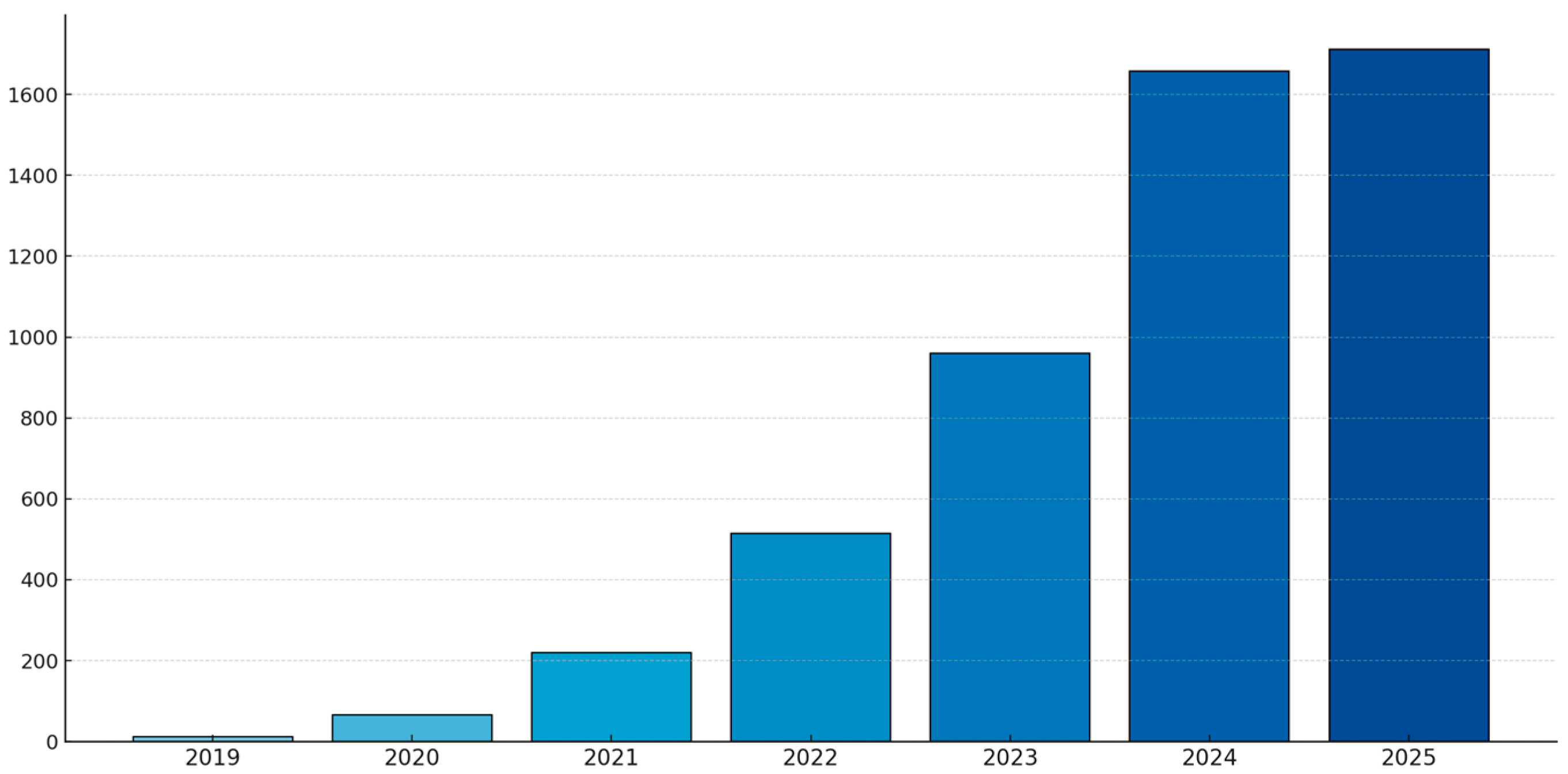
Figure 1. Dynamics of PINN publications based on Scopus database.
Mathematics 13 03289 g001
Figure 2. PINN applications [14].
Mathematics 13 03289 g002
Figure 3. Scheme of loss function formation using PINNs [30].
Mathematics 13 03289 g003
Figure 4. lbPINN neural network architecture [37].
Mathematics 13 03289 g004
Figure 5. The L 2 error versus number of training epochs for LA-PINN, PINN, and SA-PINN. Reproduced verbatim from Ref. [42]; numeric labels and symbols follow the original authors’ typesetting. Shaded bands indicate variability (±1 standard deviation).
Mathematics 13 03289 g005
Figure 6. cPINN scheme with additional conditions on interface surface [45].
Mathematics 13 03289 g006
Figure 7. PINN with identification of diffusion coefficient [54].
Mathematics 13 03289 g007
Figure 8. PINN architecture with determination of inhomogeneous material properties by separate neural networks [58].
Mathematics 13 03289 g008
Figure 9. Scheme of S-FEM-connected PINN for solving inverse elasto-plastic interaction problem [61].
Mathematics 13 03289 g009
Figure 10. Schematic of VPINN in a Petrov–Galerkin formulation [63].
Mathematics 13 03289 g010
Figure 11. Structure of the energy-based PINN with loss function integration by elements [76].
Mathematics 13 03289 g011
Figure 12. Construction of the approximate distance function to a quarter-circular arc. The leftmost plot depicts the SDF of the circle; the trimming function is shown in the middle plot; and the rightmost plot displays the approximate distance function. Reproduced verbatim from Ref. [91]; numeric labels and symbols follow the original authors’ typesetting.
Mathematics 13 03289 g012
Figure 13. Examples of points generated in [0, 1] using different uniform sampling methods [115].
Mathematics 13 03289 g013
Figure 14. Neural network architecture in the case of HC-PINN [135].
Mathematics 13 03289 g014
Figure 15. EPINN framework for solving static solid mechanics problems. Reproduced verbatim from Ref. [138]; numeric labels and symbols follow the original authors’ typesetting.
Mathematics 13 03289 g015
Figure 16. AEPINN framework for solving solid mechanics problems [139].
Mathematics 13 03289 g016
Figure 17. Network for combining a neural SDF with a PINN [87].
Mathematics 13 03289 g017
Figure 18. Domain decomposition for PINN-FEM method [144].
Mathematics 13 03289 g018
Table 1. Summary and comparison of key architectural variants of PINNs regarding engineering modeling problems.
Architecture TypeCore ConceptAdvantagesLimitations
Basic MLP-PINNClassical multilayer perceptron architecture; loss includes PDE residuals + initial and boundary conditionsSimplicity of implementation; versatility; no mesh required; automatic differentiationImbalance of loss function components (different scales of quantities); low convergence for complex PDE; sensitivity to hyperparameters
MLP-PINN with adaptive weight determination (lbPINN, SA-PINN, LA-PINN, etc.)Weight coefficients in the loss functions are determined dynamically (minimax optimization, softmax, attention mechanisms, probabilistic models)Automatic balancing of PDE/BC/IC; reduced risk of any single term dominating; improved convergence for nonlinear PDEs; effective for multiphysics problemsIncrease in optimization complexity; need for additional parameters (attention models, masks); increased computational cost
MLP-PINN with domain decomposition (cPINN, XPINN, FBPINN, PDD, etc.)Division of the area into subdomains; separate networks for each subdomain; additional matching conditions on interfacesParallelization of calculations; scalability for complex geometries and multiscale tasks; better accuracyChoice of decomposition principles not always obvious; matching on interfaces complex; possible numerical instabilities
Variational/energy PINN (VPINN, E-PINN, etc.)Use of weak form PDE (Petrov–Galerkin) or minimization of energy functional instead of PDE residualsBetter interpretability; fewer hyperparameters; more stable optimization; efficiency for multiphysics problemsNeed for numerical integration (quadrature rules); dependence of accuracy on test space; possibility of null spaces
Variational/energy PINN with domain decomposition (hp-VPINN, E-PINN with local integrals, etc.)Decomposition of the area into subdomains with local test functions or local energy integralsFewer correlated gradients; more stable training; effective parallel implementation; high accuracy for complex PDEIncreased implementation complexity; need for correct subdomain localization; additional costs for integration
Table 2. Typical levels of uncertainty for some properties of structural materials according to ASTM standards.
MaterialPropertyTypical Uncertainty (COV, %)Standard
Steel (structural)Yield strength ( σ y ) ≈7–8%ASTM A370-24. Standard Test Methods and Definitions for Mechanical Testing of Steel Products [77]
Composites (fiber-reinforced polymers)Tensile strength along fibers ( σ t ) ≈10–20%ASTM D3039/D3039M-14. Standard Test Method for Tensile Properties of Polymer Matrix Composite Materials [78]
ConcreteCompressive strength ( f c ) ≈15–25%ASTM C39/C39M-21. Standard Test Method for Compressive Strength of Cylindrical Concrete Specimens [79]
Table 3. Comparison of key PINN variants regarding multiphysics problems.
Architecture TypeSuitability for MultiphysicsAdvantages
Basic MLP-PINNMathematics 13 03289 i001 LimitedSimplicity; quick start for simple PDEs
MLP-PINN with adaptive weight determination (lbPINN, SA-PINN, LA-PINN, …)Mathematics 13 03289 i002 HighAutomatic balancing of losses of different physical nature; improved convergence; capability for nonlinear and coupled PDEs
MLP-PINN with domain decomposition (cPINN, XPINN, FBPINN, PDD, …)Mathematics 13 03289 i002 HighSeparate networks can be assigned for different physics in different regions; good scalability and parallelism
Variational/energy PINN (VPINN, E-PINN, …)Mathematics 13 03289 i002 Very highA single energy functional naturally integrates different physics; physically consistent formulation
Variational/energy PINN with domain decomposition (hp-VPINN, E-PINN)Mathematics 13 03289 i002Mathematics 13 03289 i003 HighestCombine the physical interpretability of energy-based loss with local adaptation; work well in strongly coupled systems
Table 4. Comparison of SDF and Phi-functions in the Context of PINNs.
CriterionSDFPhi-Function
MeaningDistance from point to boundary
(with positive/negative sign).
Continuous function of mutual position of two bodies (intersection, tangency, separation).
Ease of Geometry
Specification
Suitable for single objects or
smooth boundaries.
Ideal for multi-object systems and complex combinations (intersections, unions).
Local GeometryProvides surface normal
via gradient (∇SDF).
Normals not directly extracted;
boundary defined implicitly via Φ = 0.
SmoothnessSmooth and well-differentiable
with proper approximation.
Piecewise smooth function. Contains operations (min-max), less suitable for backpropagation.
Applicability in PINNsExcellent for boundary conditions
(Dirichlet/Neumann).
Better for global geometric constraints
(non-intersection, object placement).
InterpretationMetric: “distance to boundary.”Phi-function: “degree of intersection/
separation”. Normalized phi-function: Euclidean distance between objects.
Flexibility for Complex DomainsRequires specialized methods (e.g., CSG with SDF, implicit surfaces).Naturally describes combinations
and relative objects positions.
Computational PropertiesDirect approximation, good
training stability.
More complex computations, potential
gradient instability.
Table 5. Summary and comparison of methods for incorporating geometric information in modeling using PINN.
MethodKey Idea/EssenceAdvantagesDisadvantages
PIP algorithms (Ray Casting, Winding Number, mesh-based)Use predicate functions to test whether a point belongs to the domain/boundarySimplicity; basic point-membership checks; integrates with samplingDo not provide smooth information; limited use inside loss functions; ignore curvature
Analytical SDF from geometric primitivesBuild complex shapes by combining simple analytic SDFs (min/max)Simple implementation; high accuracy; low computational cosLimited to primitives with analytic SDF; non-smoothness at switching surfaces (min/max)
SDF from triangular meshes (STL-based)Distance computed from CAD mesh facets; sign from (pseudo)normalsCAD/CAE compatibility; high accuracy; library support (Open3D, libigl)High computational cost; challenging for very large/fine meshes
SDF via Eikonal (Fast Marching, Fast Sweeping)Numerical solution of φ = 1 with φ = 0 on Ω Smooth fields without gradient blow-upLimited to polygon/polyhedron-type domains
Neural SDF approaches (DeepSDF, SAL, Neural-Pull)Train a neural network to approximate a continuous SDF from point samples/unsigned dataHighest flexibility; handles complex shapes; smooth differentiable fields; fast inference after trainingHigh training cost; large datasets needed; potential overfitting
R-functionsConstruct implicit geometry via algebraic functions with logical-algebra propertiesUniversality; analyticity; can form solution structures respecting boundary conditionsMathematical complexity; limited CAD/CAE integration at present
Phi-functions Continuous functions encoding the mutual position of two bodies (intersection, tangency, separation); usable as penalties in loss or as analytical building blocks for hard-constraint trial formsNatural for multi-object configurations and optimization/packing; enforce non-overlap and placement constraints; pair well with SDF in hybrid schemesNo local metric (normals) like SDF; piecewise-smooth due to min/max → can hinder backpropagation; requires smoothing (e.g., R-operators/soft-min)
Transfinite Barycentric Coordinates (TFC)Mean-value/harmonic-coordinate–based analytic fields; domain defined as an analytical combination of local primitives; smooth everywhereAnalytically smooth (reduces gradient-explosion risk)Applicable only to polygon/polyhedron-type domains; expensive for complex STL with many faces
Table 6. Comparative analysis of collocation point generation methods for PINNs in engineering modeling problems.
Method of Collocation Point GenerationDisadvantagesAccuracy and ConvergenceIntegration with CAD/CAE
Non-adaptive methods (uniform grid, random sampling, Latin hypercube, etc.)Inefficient for complex geometries, may require many points, limited adaptivity, risks of incomplete coverage of gradient zonesAverage, stable, but slow convergenceHigh for grids, average for others (use of bounding box or CAD meshes)
Based on PDE residuals (residual-based, including DAS-PINNs)Risk of overfitting, noisiness in early stagesHighHigh (integration with CAE for dynamic reconstruction)
Causality-guided (for unsteady problems)More complex implementation, dependence on hyperparametersHigh for dynamic systemsHigh (compatible with CAE for time simulations)
Based on PDE residual gradientHigh differentiation cost, gradient noisiness, risk of local overfitting, loss of global coverageHigh, better for fixed quantityAverage (can integrate with CAD for anisotropic strategies)
Based on loss-function residuals or energy functionalsLess common, depends on loss structureHigh for multiphysics problemsHigh (integration with energy-based CAE methods)
Using SDF or R-functions (rejection sampling, projection methods, hard constraints)Costs for computing SDF/R-functions, rejection, limitations for non-analytical formsHigh, identical satisfaction of BCs for R-functionsHigh (integration with CAD/CAE for implicit geometry and BCs)
Table 7. Analysis of methods for integrating boundary conditions into the PINN structure.
Method of Boundary Condition IntegrationKey IdeaAdvantagesIntegration with CAD/CAE
Soft-constraint PINNBoundary conditions are added to the loss function as penalty termsSimplicity of implementation; universalityLow (no direct link to CAD geometries)
Hard-constraint PINNSolution represented as a sum: one part exactly satisfies boundary conditions, the other is approximated by NNGuaranteed enforcement of Dirichlet conditions; improved accuracyMedium (CAD analytics can be integrated for simple geometries)
HC-PINN with SDF/ADFUse of signed/approximate distance functions to enforce conditions on arbitrary geometriesApplicability to complex domains; guaranteed enforcement of Dirichlet, Neumann, and Robin conditionsHigh (SDF can be generated from STL/CAD meshes)
Domain Decomposition Methods (FBPINN-HC, PINN-FEM)Decomposition into overlapping subdomains, with interface conditions enforcedScalability, combining strengths of FEM and PINNHigh (CAD → mesh → easy integration with PINN)
Hard-constraint with R-functionsConstruction of solution structures that analytically satisfy various boundary conditionsUniversality; suitability for complex and combined conditionsHighest (provided R-function construction is automated with CAD data)
Disclaimer/Publisher’s Note: The statements, opinions and data contained in all publications are solely those of the individual author(s) and contributor(s) and not of MDPI and/or the editor(s). MDPI and/or the editor(s) disclaim responsibility for any injury to people or property resulting from any ideas, methods, instructions or products referred to in the content.