Abstract
This work presents a task-oriented framework for optimizing robotic surface finishing to improve efficiency and ensure feasibility under realistic kinematic and geometric constraints. The approach combines surface subdivision, optimal placement of the workpiece, and region-based toolpath planning to adapt machining strategies to local surface characteristics. A novel time evaluation criterion is introduced that improves our previous kinematic approach by incorporating dynamic aspects. This advancement enables a more realistic estimation of machining time, providing a more reliable basis for optimization and path planning. The framework determines both the optimal position of the workpiece and the subdivision of its surface into regions systematically, enabling machining directions and speeds to be adapted to the geometry of each region. The methodology was validated on several semi-complex surfaces through simulation and experimental trials with collaborative robotic manipulators. The results demonstrate that improved region-based optimization leads to machining time reductions of 9–26% compared to conventional single-direction machining strategies. The most significant improvements were achieved for larger, more complex geometries and denser machining paths, confirming the method’s industrial relevance. These findings establish the framework as a practical solution for reducing cycle time in specific robotic surface finishing tasks.
Keywords:
robot surface finishing; collaborative robot; region-based machining; automatic surface subdivision; realistic machining time estimation MSC:
93C85
1. Introduction
Modern manufacturing environments are shaped increasingly by demands for adaptability, cost effectiveness, and rapid response to design changes. This is particularly true in domains characterized by small- to medium-batch production, where investment in rigid and specialized machinery is often economically impractical [1,2]. Traditional CNC machines excel in precision and rigidity but offer limited flexibility when product lines change frequently. Against this backdrop, robotic machining has emerged as an appealing alternative. Robots provide large reachable workspaces, reprogrammability, and relatively low investment cost, features that align naturally with flexible manufacturing requirements. Their value is most pronounced in finishing operations on free-form surfaces, where adaptation to new geometries is required with minimal reconfigurations [3]. Collaborative robots (cobots) have accelerated interest in robotic machining further. Their user-friendly programming, lighter structures, and intrinsic safety features, make them attractive for deployment in environments where humans and machines must share tasks. Yet, the same design traits that support safe human interaction present difficulties for machining applications. Compared to conventional six-axis industrial arms, cobots usually have smaller payload capacities, lower stiffness, and stricter limits on joint speeds and accelerations [4].
In robotic surface finishing, the task efficiency from the robot’s kinematic standpoint is highly dependent on the selection of path direction and machining speed. A poor choice of machining direction or speed can lead to infeasible joint velocities, frequent saturations, or unnecessarily long machining times. Conversely, task-oriented optimization of these parameters has the potential to reduce processing time significantly, while ensuring feasibility within the robot`s limits [5]. This observation has motivated a substantial amount of research into kinematic performance indices, workpiece placement optimizations, and task-oriented path planning. Correct positioning of the workpiece within the robot’s workspace can reduce joint stress, avoid singularities, and improve local stiffness. Various approaches have been proposed, including the optimization of an maximal achievable end-effector velocity along a given toolpath [6]. More recently, workpiece placement has also been incorporated directly into the machining process optimization, where it serves not only to improve kinematic feasibility, but also to enhance accuracy, stability, and overall process efficiency [7]. While these strategies improve feasibility, their impact on machining time is typically indirect, as they primarily address various other constraints rather than machining time.
Traditional CAD/CAM toolpaths, designed for CNC machines, generally neglect robot-specific limitations. As a result, methods have been developed that adapt feed directions, tool orientations, and trajectory layouts to robot kinematics [8]. In parallel, vector field–based methods were developed originally for five-axis CNC machining, where surface geometry is used to construct continuous direction fields, and streamlines derived from these fields guide the machining toolpath [9]. More recently, these ideas have been extended to robotic machining. In [10], they combined pose optimization with vector-field-guided path planning, integrating surface geometry with robot kinematics to generate feasible trajectories that enhanced machining stability and accuracy when compared to conventional paths. A persistent limitation of vector field–based approaches, however, is that the preferred feed directions often vary significantly across a free-form surface. When large directional changes occur, the resulting toolpaths may suffer from discontinuities or abrupt orientations, which complicates maintaining globally optimal cutting directions [8]. This is one challenge that has motivated the development of surface subdivision techniques, where the surface is partitioned into sub-regions with more uniform geometric and kinematic characteristics, thereby improving the consistency of the machining direction.
In CNC machining, region-based subdivision has been primarily employed to minimize machining time by adapting milling parameters within each region. In [11], the subdivision was performed using a K-means clustering algorithm to group surface patches with similar geometric features, followed by maximizing the average machining strip width within each region to enable more efficient toolpath generation. Later, a similar concept was applied by combining fuzzy C-means clustering with curvature-based classification, demonstrating that precise surface partitioning can significantly reduce machining time and toolpath length [12]. In [13], an energy-aware sub-regional milling method for free-form surfaces was proposed to simultaneously improve machining efficiency and reduce energy consumption. Regions were defined by curvature features, with further subdivision using K-means clustering to group surface patches of similar shape. Within each sub-region, toolpaths were optimized using an adaptive dynamic genetic algorithm, balancing energy and time objectives under spindle power, torque, and surface roughness constraints.
Recently, several region-based robotic machining approaches have been proposed, each tailored to the needs of specific applications. Liao et al. [14] presented a method for robotic milling focused on improving machining quality through stiffness optimization. In this study, regions were defined by spectral clustering of cutter-contact points based on high-stiffness postures. The feed direction within each region was then aligned to maximize tangential stiffness, resulting in better quality and reduced depth-of-cut errors. A region-based strategy for robotic belt grinding was later introduced in [15] to avoid local gouges and simplify toolpath generation. Here, regions were defined by machinability indices derived from curvature and gouge probability analysis, distinguishing between areas suited for wheel-face and wheel-edge grinding. A two-stage clustering strategy was employed: rough partitioning into four gouge-probability levels, followed by fuzzy C-means clustering to define regions based on geometry curvature and surface normals. By using these “easy-to-grind” regions, the achieved toolpaths are comparable to those produced by skilled operators, thereby improving both efficiency and surface quality. Robotic grinding of complex stone surfaces was addressed in [16], where the author defined a machining complexity index combining curvature, area factor, and the ratio of tool diameter to minimum curvature. Surfaces are first coarsely divided by their curvature values and then refined using the fuzzy C-means algorithm. Machining direction is not optimized explicitly; instead, process parameters (feed, spindle speed, widths/depths) are chosen via a weighted summation trade-off between machining time and roughness. Finally, in [17], a region-based path planning method for robotic curved-layer wire and arc additive manufacturing was developed, aiming to maintain all welding in a horizontal position to counteract gravity effects and achieve uniform bead geometry. Regions were defined based on local geometry features using a two-stage clustering approach: subtractive clustering to estimate the number of clusters, followed by fuzzy C-means refinement. Within each subregion, machining paths were generated as offset curves from contour lines across cluster centroids, combined with a modified overlapping model that adapted the bead width to the local inclination. The regional subdivision ensured reduced surface waviness and stair-step effect, improving forming appearance and uniformity across complex geometries.
While CNC region-based machining has traditionally emphasized minimizing machining time, robotic region-based methods pursue more application-specific objectives such as stiffness improvement, gouge avoidance, surface quality, or weld uniformity. The problem, however, is that none of these strategies directly target machining time optimization based on the robot’s kinematic and dynamic capabilities in relation to the geometry of the free-form surface. This limitation becomes especially critical in time-consuming applications with dense machining paths, such as robotic machine hammer peening, where machining time constitutes a dominant factor in process efficiency. To address this issue, a recently proposed formulation of kinematic analysis embeds the constraints of the workpiece surface into the robot motion [18]. This extension builds upon the classical notion of manipulability, originally introduced by Yoshikawa [19], but adapts it to a reduced-dimensional setting defined by the surface tangent plane. By enforcing the surface constraint, the resulting measure provides a more realistic estimate of the robot’s achievable motion capabilities, expressed in terms of feasible velocities along the constrained directions.
Building on this theoretical foundation, we previously developed a method that integrates task-oriented kinematic analysis with optimal machining speed and direction selection [20]. The approach utilizes the Machining Time Index (MTI) to estimate machining cycle time and employs this evaluation to guide the generation of time-efficient region-based toolpaths. By subdividing the surface into regions with similar geometric and kinematic characteristics, the method allows each region to be machined under conditions that maximize machining efficiency. Furthermore, optimal workpiece positioning was determined, enabling the robot to maintain configurations that balance reachability and velocity performance. Together, these elements provided a systematic framework for machining time reduction in simulated robotic surface finishing.
While the original framework proved effective and demonstrated substantial time savings in simulation studies, further refinement was necessary to improve the predictive accuracy and adaptability under real-world conditions. In particular, the initial formulation of the MTI was limited to purely kinematic considerations, whereas practical machining performance is significantly affected by the dynamic aspects of robot motion. Similarly, the subdivision process relied on a manually selected number of initial clusters in the K-means algorithm for generating the final machining regions, which limited the adaptability to different surface geometries. To address these limitations, the present study introduces several key improvements that extend our earlier study and enhance its applicability in real-world robotic machining. The main contributions of this paper are as follows:
- Improved Machining Time Index (MTI): added extension to incorporate dynamic aspects of robot motion for more realistic estimation of machining time.
- Automated region subdivision: cluster number selection and generation is embedded in the MTI optimization loop, producing final machining regions without manual input.
- Extensive experimental validation: validation on a physical collaborative robot with multiple workpieces that confirms the predictive accuracy of the refined MTI and the machining time reductions achieved by the proposed framework.
By incorporating these improvements, this paper bridges the gap between simulation-based optimization and real-world robotic machining performance, providing a more reliable framework for reducing machining time on collaborative robots.
The remainder of this paper is structured as follows. Section 2 introduces the preliminary work and theoretical background, covering the differential geometry of surfaces, robot kinematics, and the determination of optimal machining directions. Section 3 presents the methodology, where the Machining Time Index is defined as the main objective function, the surface subdivision procedure is described briefly, and the optimization of workpiece optimal placement and number of clusters is outlined. Section 4 provides the case study, including the optimization and subdivision results for several representative workpieces, toolpath planning, experimental validation, and an additional scalability study with enlarged workpieces. Section 5 concludes this paper with a discussion of the main findings and directions for future work.
2. Preliminaries
2.1. Differential Geometry
In this subsection, we recall fundamentals from the differential geometry of surfaces that are required in the present work, as well as in our previous studies [18,20]. A smooth surface can be represented as a parametric mapping:
where are parameters spanning the surface domain [21]. In many practical cases, the surface can also be given explicitly by specifying the z-coordinate as a function of the in-plane xy-coordinates:
with denoting a real-valued function that is at least twice continuously differentiable. By setting and , the parametrization may be simplified to:
The outward unit surface normal vector at a given point on the surface is defined by surface’s tangent vectors and , which are the first partial derivatives of the surface parametrization :
The first fundamental form characterizes the local metric of the surface, and is defined by the matrix [22]:
with the coefficients defined as , where is the vector dot product operator.
The second fundamental form captures how the surface bends relative to its normal direction, and is given by [22]:
The second form coefficients are expressed as . Here, denote the second partial derivatives of the surface parametrization .
An important geometric property of a surface is its curvature, which describes how strongly the surface bends or deviates from being planar. The primary tools for measuring surface curvature are the first and second fundamental forms, which contain all the necessary information about the local curvature. From these, scalar measures can be derived that quantify the extent of bending of the surface at a given point. The two important measures are Gaussian curvature [23]:
and Mean curvature [23]:
where and denote the maximal and minimal principal curvatures of the surface, which can also be calculated directly from the Gaussian and Mean curvatures as [23]:
The principal curvatures play a central role in characterizing the local surface geometry. In the context of robotic region-based machining, they are particularly useful for defining clustering features in a clustering algorithm, since they provide robust descriptors of how the surface bends locally. Then, the normal curvature measures how the curve lying on the surface bends with respect to the surface normal. Its value depends on the orientation of the tangent direction relative to the principal curvatures (9) and (10). If the tangent makes an angle with the principal direction associated with , Euler’s formula gives [21]:
The geodesic torsion measures how the surface normal twists when moving along the curve. For the same angle is expressed as [21]:
2.2. Robot Kinematics
The velocity of a robot’s end-effector in Cartesian space is obtained from the joint velocities through the standard kinematic relation [24]:
where is the geometric Jacobian matrix, mapping the joint velocity vector into the operational velocity twist vector , which consists of both the linear velocity and angular velocity . For further analysis and to distinguish the linear from angular effects, it is convenient to decompose the Jacobian into translational and rotational submatrices and :
In robotic machining with a six-degree-of-freedom manipulator, the Jacobian plays a central role in determining whether the end-effector can achieve the required velocity for a given task. Solving the inverse kinematics problem requires computing the joint velocities from a desired Cartesian twist, where the Jacobian matrix must be full-rank and non-singular:
The manipulability concept is often used to quantify how effectively a robot can generate motion in arbitrary directions, which is quantified using the Jacobian matrix of the system. This is expressed through the condition [25]:
which maps the joint velocity unit sphere onto an ellipsoid in the task space, described by [26]:
2.3. Evaluation of the Maximum Feasible Speed
In free-form robotic surface machining, the end-effector must advance along a predefined trajectory, and adjust its orientation to remain aligned with the local surface geometry. Evaluating whether a given toolpath is feasible requires determining the maximum linear speed at which the tool can move while maintaining the necessary synchronized rotation. The DTF method [5] provides a task-oriented framework for this evaluation. The key idea is to separate the translational and rotational contributions of the Jacobian, and to compute the achievable speeds in a physically consistent way.
If we define a strong translational Jacobian [27], where the angular velocity is forced to zero, i.e., , and a strong rotational Jacobian [27] where the translational velocity is forced to zero, such that , the corresponding block inverse form of the Jacobian can then be written as:
where operator stands for the Moore-Penrose pseudoinverse of a matrix.
For a prescribed toolpath direction defined by unit vectors in the linear direction and angular direction , the maximum feasible translational speed can be expressed as:
The synchronization parameter reflects the ratio between the translational and rotational requirements of the tool motion, and can also be determined directly from the geometry of the workpiece surface [6]:
where is the normal curvature (11), the is geodesic torsion (12), is the magnitude of translational velocity, and is the magnitude of angular velocity.
This formulation can provide a purely geometric determination of the synchronization parameter , independent of the actual velocity scaling.
To account for the fact that the toolpath is constrained to lie on the surface of the workpiece, an augmented inverse Jacobian is used instead of the unconstrained form, which incorporates differential characteristics of the workpiece surface [18]:
where and are strong translational and strong rotational Jacobian matrices [27], and , are defined by (22) and (23), respectively [18].
Matrix maps a 2D linear velocity vector in the Cartesian plane to a 3D velocity vector in the Cartesian space, whereas maps a 2D linear velocity vector in the Cartesian plane to a 3D angular velocity in the Cartesian space. By constraining the robot motion to remain on the workpiece surface and enforcing continuous alignment of the tool with the surface normals, the augmented inverse Jacobian projects the full six-dimensional space of end-effector velocities (17) onto the two-dimensional tangent plane. This projection reduces the manipulability ellipsoid to an in-plane ellipse, eliminating the unit inconsistency that arises when mixing linear and angular velocity components and ensuring that all feasible tool velocities are expressed consistently within the tangent plane. More detailed derivations and explanations can be found in [18].
2.4. Searching for Optimal Machining Speed and Direction
At each surface point the searched two-dimensional Cartesian direction vector is projected into the tangent plane of the workpiece surface by the mapping operator , which then yields the normalized three-dimensional Cartesian direction:
The vector is then used subsequently to evaluate the maximum surface-constrained feasible speed at which the robot surface finishing can occur at each point, which is expressed as:
where is the constrained inverse Jacobian matrix defined in (21).
Since the maximum feasible speeds vary across different surface points, the optimal global machining direction must be chosen based on the worst-case local speed. This requirement leads naturally to a max–min optimization problem:
where denotes the optimal maximum feasible linear speed on the surface at the optimal direction , and is the number of the surface points under consideration.
By evaluating these optimal values across the surface, one obtains a velocity vector field (VVF) that combines both direction and speed information, providing the foundation for the subsequent path-planning procedures.
3. Materials and Methods
3.1. Improved Machining Time Index
To evaluate the efficiency and time demand of robotic surface machining processes, a Machining Time Index (MTI) was introduced in our previous study [20]. The MTI provides a comprehensive estimate of machining time, by combining the robot’s kinematic limits with the distribution of machining points on the workpiece surface. In its original formulation, the MTI served as a practical tool for comparing different path-planning strategies under simulation conditions.
However, when validated on a real robotic system, the initial MTI formulation proved to be sub-optimal. While simulations assumed idealized motion profiles, the execution on the physical robot revealed additional time losses caused by the acceleration and deceleration phases, inter-segment transitions, tool retractions, and movements between surface regions. As a result, the original MTI underestimated the actual machining times systematically.
To address this limitation, we improved the MTI by explicitly incorporating penalty terms that capture the dynamic motion and technological constraints of the real process in region-based machining. The improved index is defined as:
where:
- represents the base MTI under constant machining speed,
- accounts for the robot acceleration and deceleration effects,
- penalizes discrete tool stepovers along the machining path,
- captures intermediate tool lifts and non-cutting movements,
- represents additional time required for transitions between regions.
Figure 1 illustrates the main motion elements of the tool during machining, which are considered when forming the MTI. The red and green arrows with associated lines indicate the tool entry and exit, which are penalized with . The yellow lines represent free intermediate motions, accounted for by the penalty term . The blue lines correspond to machining toolpaths, where the acceleration and deceleration at each segment are considered with . Finally, the green lines mark individual tool stepovers with machining stepover distance , whose execution time is penalized with .

Figure 1.
The main motion elements of the tool during surface machining.
The baseline MTI is defined as the ratio between the estimated machining path length and the optimal maximum feasible speed along this path:
where present the weighting factor of machining density with respect to the stepover distance , and which is the standard distance between points. is the number of points on the workpiece surface, whereas (26) is the maximum feasible linear velocity in the tangent plane attached to the machining point on the surface of the workpiece.
In the real process of robotic surface machining, the robot cannot reach the desired machining speed immediately due to acceleration limits. Therefore, it is necessary to consider time losses caused by acceleration and deceleration, which depend on the length of the individual machining paths [28]. The total number of machining stepovers , can be estimated from the width of the region in the direction of cross-projected paths and the selected machining stepover distance :
To obtain the region width, lengths of individual machining paths, and the number of passes , the polyshape and intersect functions in the MATLAB 2023b environment were used, which enabled calculation of the intersections between the projected machining lines and region boundaries. The procedure includes (i) generating parallel lines (paths) in the optimal machining direction at uniform spacing , (ii) calculating the intersections of these paths with the machining region, defined as a polygonal region, (iii) determining the length of each machining path segment, (iv) estimating the number of stepovers, where each path segment represents one machining stepover. Figure 2 shows the generated parallel lines in the optimal machining direction with blue dashed lines. These extend across the entire region to define potential machining paths. The red solid lines indicate the machining lines detected within the region, resulting from the intersection of the generated lines with the region boundaries. The red dashed lines represent identified gaps and the black line represents the region boundary, which constrains the feasible machining area. This process represents the successful detection and estimation of machining lines/paths and the calculation of their lengths.
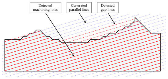
Figure 2.
Detection of intersections and calculation of machining path lengths.
Each of these red machining lines has a defined length , which depends on the region’s geometry and the machining direction. However, the robot requires a certain distance to accelerate to the desired machining speed under the given acceleration . Therefore, the threshold length of a segment is defined as:
The machining paths are then divided into:
- Long segments (), for which the speed is reached. Nevertheless, it is still necessary to account for the acceleration and deceleration times at the beginning and end of each segment, given by:where is the number of long segments.
- Short segments (), for which the robot cannot reach the constant optimal speed due to limited space. The time penalty is therefore defined as:where is the number of short segments.
Finally, the total penalty due to acceleration and deceleration is expressed as:
For each transition of the robot between machining paths (stepovers), the corresponding travel time must also be considered:
where denotes the machining stepover speed.
In machining, additional free motions may occur when, due to the machining direction and the region’s shape, the robot must stop, lift the tool, perform a rapid move, and then resume machining. These actions introduce additional time losses. The total penalty can be expressed as:
where is the acceleration or deceleration time needed to reach the rapid speed under acceleration :
and represents the travel time at constant rapid speed :
where is the remaining distance of the gap length after subtracting the acceleration and deceleration distances at both ends. In this distance, the robot can travel at a constant speed :
here, is the average length of all the paths outside the machining regions (gaps), and is the distance the robot requires to accelerate from standstill to the rapid move speed:
The time required for tool approach and retraction within each region must also be considered in region-based machining. A conservative estimate is used here, where the time for entering and exiting each region is approximated as , which is then expressed as:
where represents the number of final machining regions.
The MTI can be calculated for the entire workpiece without subdivision into regions or individually for each region, where directions and corresponding machining speeds are adapted locally. The overall MTI of the workpiece is then the sum of the regional indices, with lower values indicating shorter machining times.
The MTI can also evaluate machining efficiency for any arbitrary machining direction and workpiece placement. This enables comparison across different setups, but the index can also serve as an optimization criterion for finding the optimal workpiece position. In this way, its value can be minimized systematically to improve machining time utilization, as described in the following sections.
The main advantage of the MTI index should lie in its predictive capability, providing an estimate of machining time before the process is executed. This allows for efficient evaluation and optimization of the machining parameters before performing costly experiments on physical setups, thereby reducing production costs and shortening the development cycle of machining procedures.
3.2. Surface Subdivision
The subdivision of a workpiece can be an important step in planning robotic surface machining, as it enables the partitioning of complex geometries into smaller and more manageable regions. The procedure of surface subdivision follows the same general approach as in our previous study, where we employed K-means clustering [20]. However, two modifications were introduced in the present work. The first concerns the definition of the multidimensional feature vectors , which serve as the input to the clustering algorithm. Through extensive testing on multiple workpieces, it was found that replacing the minimal and maximal feasible speed values with the principal curvature values (,) yielded more stable clustering across different geometries. Accordingly, the new feature vector is defined as:
where the surface point components are expressed in the Cartesian coordinate system , as well as the surface normals .
To summarize, the clustering procedure is based on the input parameter , which defines the desired number of clusters for the K-means clustering algorithm. This initial clustering results in a set of clusters , with the actual number of clusters denoted as . Since a single cluster may consist of several disconnected sub-clusters, these sub-clusters are analysed and merged into the final machining regions , whose number is denoted as . This process can be expressed as: . The values of and do not necessarily coincide with the input parameter . Differences may occur, due to the spatial disconnection of individual clusters and the merging of small regions into larger ones for more practical machining regions [20].
The second modification introduced in this study concerns determining the optimal number of clusters for the input into the K-means clustering algorithm. If is set too low, the resulting clusters become excessively large, which may lead to a loss of detail and a non-optimal distribution of the final machining regions. Conversely, choosing an excessively high number of clusters increases the overall complexity of the process, and may result in unnecessary tool movements between machining regions, affecting the overall machining time negatively. Several classical methods for estimating the optimal number of clusters are available in MATLAB’s evalclusters function for the K-means clustering. However, these approaches typically favor the maximum possible number of clusters and optimize only mathematical criteria, without considering the practical objectives of robotic machining. As shown in our previous work and confirmed by other studies [29], the determination of is often subjective and context-dependent, meaning that domain knowledge and application-specific goals must guide the final choice rather than relying solely on statistical indices.
However, the manual selection of can be impractical, time-consuming, and not always optimal. To address this, in the present work, we adopted an application-oriented approach. Instead of determining the number of clusters separately and manually, we integrated it into the optimization procedure directly for finding the optimal workpiece placement. This resulted in formulating a multidimensional optimization problem, in which the number of clusters is treated as a decision variable optimized simultaneously with the workpiece position and orientation. The optimization objective is to minimize the overall machining time index (MTI). In this way, a balance is achieved between clustering complexity and machining efficiency, while the final number of clusters is not pre-defined manually, but emerges naturally as a result of the numerical optimization. The details of this optimization procedure and the definition of the objective function are presented in the following section.
3.3. Optimal Workpiece Placement and Number of Clusters
Due to the reduced mechanical capabilities and kinematic constraints of collaborative robots compared to classical industrial robots, the finding of the appropriate workpiece placement becomes a critical factor in ensuring the successful execution of robotic tasks such as surface machining. In machining processes that rely solely on the geometric model of the workpiece surface, as in our study, no pre-defined robotic toolpath is available. Instead, the process is represented only by discrete model points on the surface. Consequently, it is necessary to establish a criterion for evaluating each possible workpiece placement in terms of the efficiency of the entire machining process. This criterion must account explicitly for the influence of the robot speed limitations and provide an estimate of the overall efficiency of machining, thereby serving as the objective function in the optimization procedure.
The workpiece is described in its local coordinate system, which is positioned at its center, and is transformed with respect to the robot’s base coordinate system. The placement of the workpiece relative to the robot base is parameterized by three optimization variables . Here, and represent the Cartesian offsets of the workpiece center relative to the robot base, while denotes a rotation of the workpiece around the z-axis. The z-coordinate is fixed, representing the constant distance between the robot base and the workpiece center.
In addition to the placement parameters, the optimization also includes the variable , which defines the input number of clusters for the K-means clustering algorithm. After the merging steps, these clusters determine the number of final machining regions. The choice of influences the total machining time directly, since it enables localized adaptation of machining direction and speed according to the geometric complexity of each region. Thus, the optimization problem is formulated as a multidimensional minimization of the total Machining Time Index (MTI), defined earlier in (27). The overall objective function can be written as:
with the following constraints: (i) the robot joint angles must be within the limits, (ii) the workpiece must be positioned within a working area, (iii) the number of clusters must lie within the admissible range , (iv) for all points on the workpiece the inverse kinematic (IK) solution must exist, (v) there must be no robot self-collisions or collisions with the environment (vi) the workpiece must be on the working area with its full area.
By respecting these constraints, the optimization algorithm determines the workpiece’s placement and the number of clusters , that minimize the overall machining time while ensuring an optimal utilization of the robot’s working capabilities.
Below, Algorithm 1 presents a simplified form of the optimization program, written in pseudocode. In Step 9, the procedure of surface subdivision into regions is executed, resulting in the final number of regions . For each region, the optimal direction and the maximum feasible robot velocity are then determined according to the criterion function (26). Finally, the total MTI (27) is computed, which represents the main output of the objective function.
| Algorithm 1: Optimal Workpiece Placement and Number of Clusters |
| Input: workpiece placement () and number of clusters Output: objective function Start 1. Load and initialize the workpiece model 2. for each surface point : 3. Compute differential geometry and robot kinematic parameters 4. Solve inverse kinematics (IK) and check collisions 5. if IK is unsolvable for any point or collisions are detected 6. restart with new parameters 7. end 8. Compute Jacobian matrices 9. Apply K-means surface subdivision 10. for each region : 11. compute the objective function 12. end 13. Compute the final objective function value End |
4. Case Study
This case study evaluates the improved region-based surface machining method against the traditional single-direction machining approach. After optimizing the workpiece placement and number of clusters, the machining paths were generated using the Velocity Vector Field (VVF). Then, experimental tests were made on multiple workpieces, to assess the machining times, joint feasibility, and scalability of the method.
Figure 3 shows the three workpieces considered in this study, each with the dimensions of 200 × 200 mm (L × W). The first workpiece features a uniformly curved surface with a single dominant peak with high mean curvature values marked in blue. The second workpiece is more irregular, characterized by an extended shallow surface with the lowest mean curvature values. The third workpiece presents two evenly shaped peaks with the highest mean curvature values marked in dark blue. These three geometries were selected deliberately, to represent distinct curvature scenarios—low, medium, and high complexity—thus enabling a systematic evaluation of the proposed method’s performance under different surface conditions. This allowed us to assess both the robustness and general applicability of the approach.
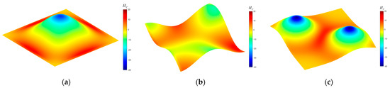
Figure 3.
Workpiece geometries analyzed in this study denoted by mean curvature values. Blue color marks high curvature and red color marks low curvature: (a) Workpiece 1 (WP1), (b) Workpiece 2 (WP2), (c) Workpiece 3 (WP3).
4.1. Surface Subdivision and Optimization Results
Optimization using the Particle Swarm Optimization (PSO) algorithm [30] was employed to maximize the objective function for identifying the optimal machining speeds and directions within the overall optimization , which, simultaneously, determines the optimal workpiece placement and the optimal number of clusters for surface subdivision. Considering the trade-off between computational complexity and the desired quality of machining, the machining stepover distance was set to in all the optimization cases, which represents a balanced compromise value. The minimum number of input clusters was set to , while the maximum number of clusters was limited to , since higher values of proved in a previous study to be inefficient in practice.
The additional optimization constraints were: (i) the UR5e joints angles were limited within the range , (ii) the working area was constrained by and , (iii) workpiece rotation was enabled in a full range of .
4.1.1. Workpiece 1
The final optimization result for WP1 includes the optimal placement with coordinates XYZ = [−46; −564; −96] (mm) with respect to the robot’s reference coordinate system, with a rotation around the Z-axis of 253°. The optimal number of clusters was determined as , resulting in a final number of machining regions . The figure below presents a comparison between the single-direction optimal machining (Figure 4a), where the overall machining speed was evaluated as , and the regional subdivision, with corresponding optimal machining directions (VVF field) and the associated maximum feasible machining speeds for each region (Figure 4b). Figure 4c shows a 3D visualization of the regional subdivision together with the VVF field and the maximum feasible machining speeds in each region.
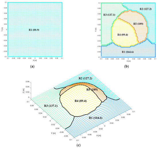
Figure 4.
Comparison of single-direction optimal machining and region-based optimal machining for WP1, showing the maximum feasible speeds (mm/s) and the VVF field: (a) single-direction optimal machining, (b) region-based machining, (c) 3D view of region-based machining.
It is important to emphasize that optimization is based on a discrete evaluation with a machining stepover distance of 2 mm, while, in reality, different stepover distances can be applied. Since the number of passes and the total path length change with the stepover distance, this could theoretically influence the optimal number of clusters and regions. However, the results presented in Table 1 confirm that for WP1, the optimal number of input clusters marked in bold remains constant, even when different machining stepover distances are considered, which is also reflected in the same number of final regions. The table also shows the percentage improvement of the most favorable region-based case compared to single-direction, where the MTI indicates that, with a 4 mm machining step, the benefit of regional subdivision is negligible (1.1%), but decreasing the stepover distance makes the use of regions increasingly more justified (up to 24%).

Table 1.
Comparison of the MTI values for different machining stepover distances and numbers of input clusters for WP1. The improvement (%) represents the difference between the optimal number of clusters and a single cluster.
4.1.2. Workpiece 2
The optimal placement for WP2 was found at the coordinates XYZ = [9; −513.4; −96] (mm) relative to the robot’s reference coordinate system, with a rotation around the Z-axis of 347°. For a machining stepover distance of 2 mm, the optimal number of clusters was determined as , which means that, for WP2, the best result was achieved with optimal single-direction machining at the optimal speed, without regional subdivision. In this case, the additional subdivision into regions did not contribute to reducing the machining time. Figure 5a shows the results of single-direction optimal machining with a speed of , compared with the best regional subdivision (Figure 5b), where .
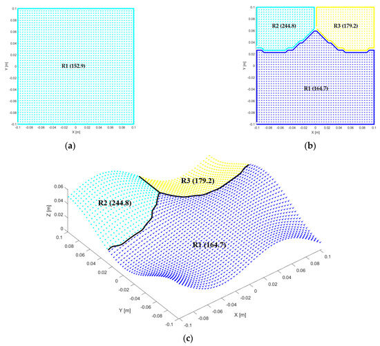
Figure 5.
Comparison of single-direction optimal machining and region-based optimal machining for WP2, showing the maximum feasible speeds (mm/s) and the VVF field: (a) single-direction optimal machining, (b) region-based machining, (c) 3D view of region-based machining.
The results for different numbers of clusters and machining stepover distances (ranging from 4 mm to 0.1 mm), presented in Table 2, confirm further, that for WP2, regional subdivision according to the MTI only became theoretically meaningful at a very small stepover distance of 0.1 mm. Even then, the improvement remained marginal (4.4%). This indicates that, for this particular workpiece, regional subdivision is not recommended in practice, since the additional complexity of the method does not yield a sufficient reduction in machining time compared to optimal single-direction machining.
Table 2.
Comparison of the MTI values for different machining stepover distances and numbers of input clusters for WP2. The improvement (%) represents the difference between the optimal number of clusters and a single cluster.
4.1.3. Workpiece 3
For WP3, we performed optimization of both the placement and the number of clusters similarly. The optimal configuration was found at coordinates XYZ = [105; −552; −96] (mm) relative to the robot’s reference coordinate system, with a rotation around the Z-axis of 328°. The optimal number of clusters was determined as , resulting in a total of final machining regions. This workpiece features a more complex and highly curved surface, similar to WP1, where regional subdivision was particularly effective, as it enabled better adaptation to the local motion constraints of the robot, and thus more efficient path planning.
Figure 6 shows the results of the regional subdivision compared with optimal single-direction machining. The results in Table 3 indicate that the use of regions is beneficial, even at a coarse machining stepover distance of 4 mm, where the MTI improvement compared to single direction machining reached 14.1%. For smaller stepover distances, the improvements increased gradually, demonstrating the growing benefit of using regions. At a stepover distance of 0.1 mm, the improvement reached 27.7%, which highlights the significant potential for reducing the machining time. In this case, the region-based approach proved to be highly effective, and can represent a key contribution to improving machining efficiency. As with WP1, the optimization indicated consistently that the optimal number of clusters remained across different machining stepover distances.
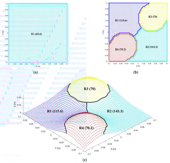
Figure 6.
Comparison of single-direction optimal machining and region-based optimal machining for WP3, showing the maximum feasible speeds (mm/s) and the VVF field: (a) single-direction optimal machining, (b) region-based machining, (c) 3D view of region-based machining.
Table 3.
Comparison of the MTI values for different machining stepover distances and numbers of input clusters for WP3. The improvement (%) represents the difference between the optimal number of clusters and a single cluster.
4.2. Path Planning
The machining paths were generated in Autodesk Fusion 360 CAM (version 2603.1.15) using the Steep and Shallow strategy, which enables five-axis machining with automatic adaptation of the tool orientation normal to the local geometry of the workpiece surface. In this way, a generic toolpath was created in the APT (Automatically Programmed Tool) format, which can be transferred independently to workpieces in different placements. For transferring the CAM program into a robot program, the simulation and post-processing environment RoboDK (version 5.7.4) was used, enabling transformation of the toolpath into executable commands for the target robot—in this case, the UR5e. In this study, a parallel (zig-zag) toolpath strategy [31] was applied, which is a commonly used technique in robotic surface finishing.
In practical machining, several technological motions must be considered, each executed at different speeds. First, there is the tool approach motion toward the workpiece before machining begins, and the tool retraction after machining ends, both performed at the machining speed assigned to the specific region or to the entire workpiece. The rapid free motion refers to tool movement through free space, without material removal, when transitioning between different regions of the workpiece; this is usually carried out at higher speeds to minimize non-productive time. In our case the speed was set to 150 mm/s. The stepover speed defines the tool speed when moving between adjacent toolpaths or stepovers, which is typically slower, set at 20 mm/s. In this study, the stepover distance between successive passes was set in the range of 0.1 mm to 2 mm, corresponding to values typically employed in high-precision surface finishing operations.
Within this setup, machining paths were generated for several different scenarios across the three workpieces:
- Arbitrary single direction machining: Machining is carried out strictly along the global X and Y axes, as shown in Figure 7a–f. This scenario represents a traditional approach, in which the tool moves linearly across the workpiece surface, without considering surface topology, robot kinematics, or any optimization criteria.
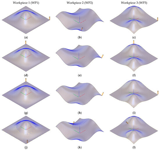 Figure 7. Comparison of the different machining paths for three workpieces, WP1 (left column), WP2 (middle column), and WP3 (right column), in their optimal placements: (a–c) machining in the X-direction, (d–f) machining in the Y-direction, (g–i) machining in an optimal single-direction, (j–l) machining with region-based optimal directions.
 - Single-direction optimal machining: In this case, the machining direction was determined based on the MTI calculated for the entire workpiece (Figure 7g–i). The chosen direction represents the globally most efficient direction, minimizing the overall machining time.
- Region-based optimal direction machining: here, the workpiece surface was subdivided into regions, and, for each region, an optimal machining direction and speed was calculated based on the MTI (Figure 7j–l).
Path speed validation (19) refers to the process of verifying whether the maximum feasible machining speeds predicted by our method can also be achieved along the actual toolpaths executed by the robot. Since our framework evaluates speed feasibility in the tangent plane of the workpiece, deviations may occur once these directions are mapped onto discrete robot toolpaths. In previous work, we confirmed that our method provides a reliable estimate of achievable speeds, though small deviations were observed between the predicted and realized speeds. A similar validation was performed in this study, again showing good agreement between the model and the experimental toolpaths. Nevertheless, to account for minor discrepancies and ensure safe operation, all the machining speeds used in the experiments were reduced by 10% relative to the predicted optimal values. In addition to speed validation, previous work also investigated the influence of workpiece placement. The same experiments for the current workpieces confirmed that optimizing the placement of the workpiece can yield improvements of up to 16% in machining time compared with random placements, highlighting the importance of integrating placement optimization into the overall framework.
To illustrate the outcome of the optimization procedure from Section 4.1 further, Figure 8 presents the optimal workpiece placement and corresponding optimal machining toolpaths for each of the three investigated workpieces in the simulation environment. In Figure 8a, WP1 is shown in its optimal position with region-based machining toolpaths. For WP2, depicted in Figure 8b, the optimization indicated that an optimal single-direction machining strategy is more efficient than a region-based approach. Finally, Figure 8c shows WP3 in its optimal position, where the region-based toolpaths again provide the most effective strategy.
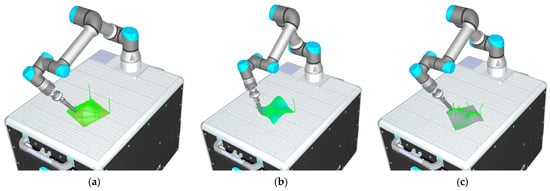
Figure 8.
Optimal workpiece placement and machining toolpaths obtained from the optimization procedure: (a) WP1 optimal region-based toolpath, (b) WP2 optimal single-direction toolpath, and (c) WP3 optimal region-based toolpath.
4.3. Experimental Results
The experimental platform was based on the Universal Robots UR5e collaborative robot, a system adopted widely in flexible, low-volume, high-mix production environments, due to its versatility and ease of deployment. The UR5e provides a reach of 850 mm and supports payloads of up to 5 kg, making it suitable for a broad range of surface finishing tasks. For our study, a 3D printed machine hammer peening (MHP) tool with a length of 284.5 mm was mounted on the robot, though the proposed method is applicable to other finishing processes where machining time optimization is critical—provided that appropriate technological parameters specific to each process are considered carefully, which lies beyond the scope of this work.
After the planning and validation of the machining paths, the robot programs were verified further and tested in the URSim simulation environment (Polyscope version 5.13), where motion analysis and time validation were carried out without any risk to the physical robot. Following a successful simulation, the machining experiments were executed on the real UR5e robotic system, with actual motion and machining times recorded through the Real-Time Data Exchange (RTDE) protocol. This allowed for a direct comparison and validation between the machining times estimated by the MTI and those obtained from real execution, serving as the basis for evaluating accuracy and analyzing the time efficiency of both region-based and traditional single-direction machining strategies.
The analysis demonstrates the efficiency of the machining strategies, particularly highlighting the advantages of the region-based approach compared to classical single-direction machining. The results for WP1 are presented in Table 4, showing that the machining time on the real system was reduced by approximately 9–23%, depending on the path density.
Table 4.
Machining time results for WP1 in the optimal placement using different machining strategies. The improvement (%) represents the difference between region-based machining and the single optimal machining path.
The analysis of MTI values between region-based and optimal single-direction machining for workpiece WP2 (see Table 2) had already indicated that regional subdivision in this case did not lead to significant improvements in the overall machining time. This finding was confirmed further by the experimental results in Table 5, which present the actual machining times under different strategies for each stepover distance (from 2 mm to 0.1 mm). It can be observed that, for none of the tested stepovers, did region-based machining achieve a substantially shorter machining time compared to machining in the optimal single direction. The reason lies in the relatively low curvature of the WP2 surface and the consequently favorable speed configuration, even when the machining was carried out in a single direction. Since the critical point that determines the maximum feasible speed in single machining was already relatively “fast” for this workpiece, this speed remained uniformly high across other parts of the surface area as well. This means that subdividing the surface into smaller regions with locally optimized directions and speeds does not provide sufficient additional benefits. It is also important to note that the optimal single-direction strategy was still determined using the proposed method. For instance, at a stepover distance of 1 mm, machining in the optimal single direction reduced the execution time by approximately 8% compared to machining strictly along the X-axis, and by as much as 32% compared to machining along the Y-axis. This highlights that, even when regional subdivision does not provide additional benefits, the systematic identification of an optimal single direction and speed can still yield significant improvements over conventional machining.
Table 5.
Machining time results for WP2 in the optimal placement using different machining strategies. The improvement (%) represents the difference between region-based machining and the single optimal machining path.
For WP3, characterized by a more complex and highly curved surface, the region-based approach again proved to be an effective machining strategy. The results in Table 6 show clearly that region-based machining outperformed optimal single-direction machining significantly. Already, at the largest stepover of 2 mm, a reduction in machining time of approximately 19% was achieved, while, at smaller stepovers this difference increased further. The greatest relative improvement was observed at a step-over of 0.1 mm, where the region-based strategy reduced the machining time by more than 25% compared to the optimal single-direction.
Table 6.
Machining time results for WP3 in the optimal placement using different machining strategies. The improvement (%) represents the difference between region-based machining and the single optimal machining path.
The overall results show that the region-based approach outperformed the other strategies in two cases (WP1 and WP3) with respect to reducing the machining time, particularly at smaller stepover distances. Although the regional subdivision was not beneficial for workpiece WP2, the results demonstrated that even the selection of an optimal single direction using our method can improve machining time compared to arbitrary machining directions.
In general, subdividing the workpiece into regions helps to avoid the bottlenecks that arise when machining the entire surface at the minimum (maximum feasible) speed determined by an arbitrary, non-optimized direction. Instead, each region can be machined at an optimized speed and direction best suited to its specific characteristics. Furthermore, the use of the developed MTI enabled a reliable preliminary estimation of the machining time, as it was shown to correlate closely with the actual machining times, and therefore represents an effective criterion for optimization.
Joint Speed Validation
To verify the practical feasibility of the path planning method based on regions, we also analyzed the actual joint angular speeds during surface machining. The primary goal was to confirm that the robot’s motions corresponded to the calculated machining speeds and that these remained within the UR5e robot’s limits, specifically not exceeding the maximum joint angular speed of .
Previous validations showed that discrepancies exist between the linear speeds predicted by the VVF model and the actual speeds along real machining paths. This deviation may reflect local exceedances of the joint speed limits. Therefore, in practical implementations, the final path speeds were determined with a safety factor—a 10% reduction relative to the calculated maximum speed was applied in this study. Figure 9 presents boxplots of the joint speeds for individual robot joints under different machining strategies with a stepover distance of 1 mm. The left column shows the results for optimal single-direction machining, while the right column shows those for region-based machining. The subfigures correspond to different workpieces: Figure 9a,b WP1, Figure 9c,d WP2, and Figure 9e,f WP3.
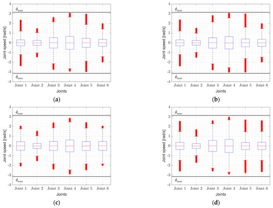
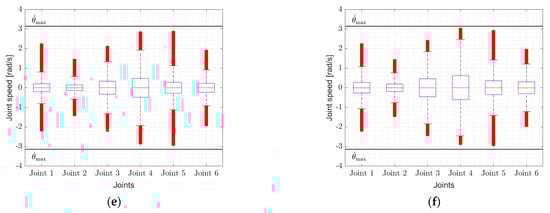
Figure 9.
Norm of joint angular speeds during robotic surface machining: (a) WP1 optimal single-direction machining, (b) WP1 region-based machining, (c) WP2 optimal single-direction machining, (d) WP2 region-based machining, (e) WP3 optimal single-direction machining, (f) WP3 region-based machining.
It can be seen that the joint speeds remained close to the upper allowable limit in all cases, but never exceeded it. This confirms that the proposed method exploits the robot’s maximum machining linear speed capabilities effectively, while respecting the maximum feasible joint speeds accurately.
4.4. Experiment with Enlarged Workpieces
In the previous experiments all the workpieces were considered at their base dimensions of 200 × 200 mm (L × W), using the collaborative robot UR5e (Universal Robots, Odense, Denmark). However, in certain scenarios, a workpiece may include relatively small machining regions where high machining speeds are feasible. In such cases, the effects of robot acceleration and deceleration become more pronounced, which can lead to relatively greater time losses and reduced overall efficiency. To investigate the influence of workpiece size on time efficiency, an additional experiment was conducted in which the original workpieces were scaled up proportionally by 50%, resulting in final dimensions of 300 × 300 mm with proportional scaling applied to the height as well. For this experiment, the collaborative robot UR10e was used, as it provides a larger reach and is thus capable of handling bigger workpieces. The UR10e robot, together with both the small and enlarged versions of WP1 mounted on the platform, is shown in Figure 10. Unlike the previous experiments performed on the physical UR5e robot, the machining times for the enlarged workpieces were obtained exclusively in the URSim simulation environment, because a physical UR10e robot was not available. Nevertheless, in all the earlier UR5e experiments, the simulator was verified to yield machining times consistent with the real robot execution, thereby ensuring the reliability of the results presented here.
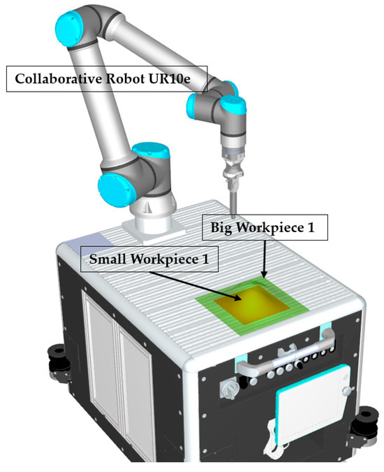
Figure 10.
Small and big WP1 on a flexible workstation with a UR10e robot.
A suitable workpiece placement was selected such that both the smaller and enlarged workpieces were fully reachable, and machining could be executed without collisions. In this fixed placement, region-based subdivision was first performed on the smaller workpiece, following the same procedure as in the previous experiments. The maximum feasible machining speeds and optimal machining directions were calculated for each region. The optimal speed and direction for single machining direction were also determined in addition to the regional approach.
Subsequently, all the calculated machining speeds and directions from the smaller workpiece were transferred directly to the enlarged workpiece. This allowed for an evaluation of how changes in the workpiece geometry affect the overall Machining Time Index (MTI), where the path length increases, and, consequently, alters the ratio between the acceleration, steady-motion, and deceleration phases.
The results of the experiment are presented in Table 7, and provide a quantitative assessment of how increasing the size of the workpiece influences the efficiency of the machining strategy, and to what extent region-based planning remains beneficial for larger geometries. In these experiments, the effect of a region-based approach with a machining step size of 1 mm was analyzed for three small and large workpieces.
Table 7.
Comparison of machining times between the original workpiece dimensions and the enlarged dimensions.
The results showed an additional improvement in machining time when using the region-based strategy on larger workpieces. In the first case, the improvement for the large WP1 was 13.6%, which is 6.4%, or 88.2% relative, greater than for the small workpiece (7.2%). In the second case, the small WP2 even showed an increase in machining time with region-based segmentation compared to optimal unidirectional machining (−3.6%), whereas the large WP2 still achieved an improvement of 1.3%. This corresponds to a difference of 4.9%, or 135.7% relative improvement. The third case showed good results for both sizes, but the large WP3 again stood out with an improvement of 23.9%, which is 3.5%, or 17.2% relative, higher than for the small WP3 (20.4%).
These results indicate that the region-based approach scales better and becomes more effective for larger workpieces, where regions are larger and toolpaths are longer. However, as already observed in some cases (e.g., WP2), the regional approach is not always effective, and may even affect machining time negatively compared to optimal single-direction machining.
5. Discussion and Conclusions
This study investigates the efficiency of region-based surface machining, in which optimal machining speeds and directions are determined for semi-complex surfaces, in order to improve the efficiency of the process compared to traditional single-direction strategies. Compared to our previous work, this study introduces an improved surface subdivision procedure, where the optimal number of clusters is determined simultaneously with the optimal workpiece placement, based on the improved Machining Time Index (MTI). The revised MTI incorporates multiple real-world factors, ensuring that the numerical results align more closely with the actual robot execution.
Our findings demonstrate that subdividing the workpiece into regions improves the machining efficiency compared to traditional single-direction strategies, reducing the machining time by 9% to as much as 26%, depending on the geometry of the workpiece and the machining stepover distance. The greatest improvements were observed at smaller stepovers, indicating that region-based strategies are particularly effective with denser toolpaths. The effects of regional segmentation were less pronounced for workpieces with less curvature and larger stepover. In such cases, workpieces may also contain so-called critical points, where the maximum feasible machining speed is already relatively high. If such a point is also representative of the majority of the surface, the robot can maintain this high speed across the entire workpiece, meaning that further subdivision does not provide additional benefits.
Nevertheless, even in cases where region-based segmentation does not provide significant improvements compared to optimal single-direction machining, the latter in our approach was not performed arbitrarily, as is often the case in industrial practice (e.g., machining simply along the X or Y direction, chosen heuristically by the operator). Instead, our method identifies the critical point on the surface systematically—i.e., the location where the kinematic requirements are the most demanding, and which largely determines the maximum feasible machining speed for the entire process. This allowed us to construct an optimal single-direction machining strategy that is considerably more efficient than random or manually selected directions.
Based on previous findings and validations, we reduced the maximum allowable robot speeds conservatively by 10%, to ensure safe operation within the robot’s true kinematic limits. Further validation confirmed that the robot’s joint angular speeds during machining remained within the permissible limits, which confirms the reliability of the proposed method for path feasibility evaluation further.
Finally, an experiment was performed with scaled-up workpieces, where the base workpiece dimensions were increased by 50%, simulating scenarios with larger machining regions. The results showed that, in such cases, regional subdivision becomes even more effective, as larger regions enable better exploitation of local kinematic constraints, and provide longer stable toolpaths within each region. This demonstrates the scalability of the method and its applicability to larger parts in industrial contexts.
Overall, the presented method enables robust and efficient path planning for robotic surface machining, by incorporating both kinematic and dynamic constraints along with the geometric characteristics of the workpiece. The method proved useful, not only in cases requiring complex regional subdivision, but also in the optimization of simple single-direction strategies, demonstrating its flexibility and potential for broader industrial implementation.
The proposed method can be readily transferred to other semi-complex or larger workpieces and robots, provided that an accurate kinematic model of the robot and a precise representation of the workpiece surface are available. While the number of surface points naturally increases with larger parts, leading to a higher computational load, the entire optimization procedure is performed offline; therefore, the increase in computation time does not pose a critical limitation to applicability in practice. Beyond machine hammer peening, the framework is also transferable to other robotic surface finishing operations such as grinding, polishing, burnishing, or milling. In such cases, however, the Machining Time Index and possibly machining strategies would need to be extended with process-specific technological parameters to accurately capture the dynamics of each application.
For future work, we plan to extend testing to other collaborative robots, especially 7-axis models, as well as to larger industrial robots designed for the processing of substantially larger workpieces. So far, the method has been validated successfully on the collaborative robots UR5e and UR10e; in the future, we aim to include more powerful platforms with additional practical experiments in industrial environments. Furthermore, we intend to adapt the method for use on geometrically more complex workpieces, and to integrate it with advanced CAM tools, which will allow for even greater accuracy and efficiency in path planning.
Author Contributions
Conceptualization, T.P.; methodology, T.P. and A.H.; software, T.P. and A.H.; validation, T.P.; writing—original draft preparation, T.P.; writing—review and editing, A.H.; supervision, A.H. All authors have read and agreed to the published version of the manuscript.
Funding
This research was funded by the Slovenian Research Agency (ARIS) under a Grant for the Research Program P2–0028.
Data Availability Statement
The original contributions presented in this study are included in this article. Further inquiries can be directed to the corresponding authors.
Conflicts of Interest
The authors declare no conflicts of interest.
References
- Löfving, M.; Almström, P.; Jarebrant, C.; Wadman, B.; Widfeldt, M. Evaluation of flexible automation for small batch production. Procedia Manuf. 2018, 25, 177–184. [Google Scholar] [CrossRef]
- Gan, Z.L.; Musa, S.N.; Yap, H.J. A Review of the High-Mix, Low-Volume Manufacturing Industry. Appl. Sci. 2023, 13, 1687. [Google Scholar] [CrossRef]
- Hahnel, S.; Pini, F.; Leali, F.; Dambon, O.; Bergs, T.; Bletek, T. Reconfigurable Robotic Solution for Effective Finishing of Complex Surfaces. In Proceedings of the 2018 IEEE 23rd International Conference on Emerging Technologies and Factory Automation (ETFA), Turin, Italy, 4–7 September 2018. [Google Scholar]
- Vitalli, R.; Fioretti, F.; Rebouças, M.; Freitas, J. A comparative study of time-related performance: COBOT with industrial robots using digital twin robotic cells. Int. Robot. Autom. J. 2024, 64, 304–309. [Google Scholar] [CrossRef]
- Stradovnik, S.; Hace, A. Task-Oriented Evaluation of the Feasible Kinematic Directional Capabilities for Robot Machining. Sensors 2022, 22, 4267. [Google Scholar] [CrossRef] [PubMed]
- Stradovnik, S.; Hace, A. Workpiece Placement Optimization for Robot Machining Based on the Evaluation of Feasible Kinematic Directional Capabilities. Appl. Sci. 2024, 14, 1531. [Google Scholar] [CrossRef]
- Kratěna, T.; Vavruška, P.; Švéda, J.; Zeman, P. Workpiece position optimisation in robotic multi-axis machining. Results Eng. 2025, 27, 106421. [Google Scholar] [CrossRef]
- Sun, Y.; Jia, J.; Xu, J.; Chen, M.; Niu, J. Path, feedrate and trajectory planning for free-form surface machining: A state-of-the-art review. Chin. J. Aeronaut. 2022, 35, 12–29. [Google Scholar] [CrossRef]
- Xie, S.; Liu, Z. A Review of Vector Field-Based Tool Path Planning for CNC Machining of Complex Surfaces. Symmetry 2025, 17, 1300. [Google Scholar] [CrossRef]
- Wu, L.; Zang, X.; Yin, W.; Zhang, X.; Li, C.; Zhu, Y.; Zhao, J. Pose and Path Planning for Industrial Robot Surface Machining Based on Direction Fields. IEEE Robot. Autom. Lett. 2024, 9, 10455–10462. [Google Scholar] [CrossRef]
- Liu, X.; Li, Y.; Li, Q. A region-based 3 + 2-axis machining toolpath generation method for freeform surface. Int. J. Adv. Manuf. Technol. 2018, 97, 1149–1163. [Google Scholar] [CrossRef]
- Liu, H.; Zhang, E.; Sun, R.; Gao, W.; Fu, Z. Free-Form Surface Partitioning and Simulation Verification Based on Surface Curvature. Micromachines 2022, 13, 2163. [Google Scholar] [CrossRef]
- Zhao, J.; Li, L.; Li, C.; Sutherland, J.W.; Li, L. Energy-aware sub-regional milling method for free-form surface based on clustering features. J. Manuf. Process. 2022, 84, 937–952. [Google Scholar] [CrossRef]
- Liao, Z.-Y.; Li, J.-R.; Xie, H.-L.; Wang, Q.-H.; Zhou, X.-F. Region-based toolpath generation for robotic milling of freeform surfaces with stiffness optimization. Robot. Comput.-Integr. Manuf. 2020, 64, 101953. [Google Scholar] [CrossRef]
- Xie, H.-L.; Li, J.-R.; Liao, Z.-Y.; Wang, Q.-H.; Zhou, X.-F. A robotic belt grinding approach based on easy-to-grind region partitioning. J. Manuf. Process. 2020, 56, 830–844. [Google Scholar] [CrossRef]
- Yin, F.-C. A Partitioning Grinding Method for Complex-Shaped Stone Based on Surface Machining Complexity. Arab. J. Sci. Eng. 2022, 47, 8297–8314. [Google Scholar] [CrossRef]
- Hu, Z.; Hua, L.; Qin, X.; Ni, M.; Liu, Z.; Liang, C. Region-based path planning method with all horizontal welding position for robotic curved layer wire and arc additive manufacturing. Robot. Comput.-Integr. Manuf. 2022, 74, 102286. [Google Scholar] [CrossRef]
- Hace, A. Toward Optimal Robot Machining Considering the Workpiece Surface Geometry in a Task-Oriented Approach. Mathematics 2024, 12, 257. [Google Scholar] [CrossRef]
- Yoshikawa, T. Dynamic manipulability of robot manipulators. In Proceedings of the 1985 IEEE International Conference on Robotics and Automation, St. Louis, MO, USA, 25–28 March 1985. [Google Scholar]
- Pušnik, T.; Hace, A. Region-Based Approach for Machining Time Improvement in Robot Surface Finishing. Appl. Sci. 2024, 14, 9808. [Google Scholar] [CrossRef]
- Patrikalakis, N.; Maekawa, T. Shape Interrogation for Computer Aided Design and Manufacturing; Springer: Berlin/Heidelberg, Germany, 2002. [Google Scholar]
- Gallier, J. Basics of the Differential Geometry of Surfaces. In Texts in Applied Mathematics; Springer: New York, NY, USA, 2011; pp. 585–654. [Google Scholar]
- Pressley, A. Elementary Differential Geometry; Springer Undergraduate Mathematics Series; Springer Nature: Dordrecht, The Netherlands, 2010. [Google Scholar] [CrossRef]
- Siciliano, B.; Sciavicco, L.; Villani, L.; Oriolo, G. Robotics; Advanced Textbooks in Control and Signal Processing; Springer: Berlin/Heidelberg, Germany, 2009. [Google Scholar] [CrossRef]
- Yoshikawa, T. Manipulability of Robotic Mechanisms. The International Journal of Robotics Research 1985, 4, 3–9. [Google Scholar] [CrossRef]
- Lynch, K.M.; Park, F.C. Modern Robotics: Mechanics, Planning, and Control; Cambridge University Press: Cambridge, UK, 2017. [Google Scholar]
- Yoshikawa, T. Translational and rotational manipulability of robotic manipulators. In Proceedings of the IECON ‘91: 1991 International Conference on Industrial Electronics, Control and Instrumentation, Kobe, Japan, 28 October–1 November 1991. [Google Scholar]
- Kim, B.H.; Choi, B.K. Machining efficiency comparison direction-parallel tool path with contour-parallel tool path. Comput.-Aided Des. 2002, 34, 89–95. [Google Scholar] [CrossRef]
- Schubert, E. Stop using the elbow criterion for k-means and how to choose the number of clusters instead. ACM SIGKDD Explor. Newsl. 2023, 25, 36–42. [Google Scholar] [CrossRef]
- Kennedy, J.; Eberhart, R. Particle swarm optimization. In Proceedings of the of ICNN’95—International Conference on Neural Networks, Perth, Australia, 27 November–1 December 1995. [Google Scholar]
- Bavaramanandi, S.K.; Patel, D.; Dodiya, H. A brief review on feed rate optimization and different type of toolpath use in pocket machining. Int. J. Tech. Innov. Mod. Eng. Sci. (IJTIMES) 2019, 5, 1103–1110. [Google Scholar]
Disclaimer/Publisher’s Note: The statements, opinions and data contained in all publications are solely those of the individual author(s) and contributor(s) and not of MDPI and/or the editor(s). MDPI and/or the editor(s) disclaim responsibility for any injury to people or property resulting from any ideas, methods, instructions or products referred to in the content. |
© 2025 by the authors. Licensee MDPI, Basel, Switzerland. This article is an open access article distributed under the terms and conditions of the Creative Commons Attribution (CC BY) license (https://creativecommons.org/licenses/by/4.0/).