Statistics of Global Stochastic Optimisation: How Many Steps to Hit the Target?

Abstract

Random walks are considered in a one-dimensional monotonously decreasing energy landscape. To reach the minimum within a region ${\Omega }_{ϵ}$, a number of downhill steps have to be performed. A stochastic model is proposed which captures this random downhill walk and to make a prediction for the average number of steps, which are needed to hit the target. Explicit expressions in terms of a recurrence relation are derived for the density distribution of a downhill random walk as well as probability distribution functions to hit a target region ${\Omega }_{ϵ}$ within a given number of steps. For the case of stochastic optimisation, the number of rejected steps between two successive downhill steps is also derived, providing a measure for the average total number of trial steps. Analytical results are obtained for generalised random processes with underlying polynomial distribution functions. Finally the more general case of non-monotonously decreasing energy landscapes is considered for which results of the monotonous case are transferred by applying the technique of decreasing rearrangement. It is shown that the global stochastic optimisation can be fully described analytically, which is verified by numerical experiments for a number of different distribution and objective functions. Finally we discuss the transition to higher dimensional objective functions and discuss the change in computational complexity for the stochastic process.

1. Introduction

Biased random walks (RW) with varying or decreasing step sizes have been studied for some time and are known in the mathematics community as Bernoulli convolutions [1,2,3]. Different scenarios have been studied for 1-dimensional (1d) systems, among them the exponentially decaying step size, which is also known as the lazy or tired random walker [4,5]. For a systematic decrease in step sizes in a random walk, some interesting properties could be obtained. For a random walk with step sizes $\delta x_n=\pm {\lambda }^{-n},0<\lambda <1$, the random walk is bound to a finite region, and for $\lambda =2^{-k/2}$, limiting density distribution functions for the end-to-end distances, i.e., the sum of random steps, could be found, which correspond to a $(k+1)$-times convolution of a uniform density distribution on $[-1,1]$ [6]. As a general result, it could be shown that for $\lambda \in [1/2,1]$, the corresponding density distribution is almost continuous, whereas in the interval $\lambda \in [0,1/2]$, the supports are discrete Cantor sets [7,8].

First passage time characteristics [9] for random walks with decaying steps in 1d systems were considered in Ref. [10], where an analogy was also considered for a continuous time random walk with a decaying diffusion constant in time. For the discrete case, values of $\lambda$ were found, where the mean first passage time undergoes transitions, which are reflected in ladder like behaviour. Later, memory effects were also studied for random walks with decaying steps [11] in d-dimensional systems, which is present in these systems due to the finite extent of end-to-end distance as the step size decays to zero. Correlations between, e.g., the direction of the first step and end-point position could be computed analytically. First passage times in 2d and 3d were considered in Ref. [12], where the exit time from a confined region was considered.

In the present article we first consider a simplified random search model in one-dimensional space for global stochastic optimisation [13,14], which follows an acceptance criterion upon a decreasing cost function. It will be demonstrated that the path between successive steps follows a biased random walk model (only downhill moves are accepted) with variable step size. It proceeds with the generation of uniform random numbers which are generated within a finite region $\Omega$ and the minimum region, ${\Omega }_{ϵ}\subset \Omega$, is searched for through trial-and-error attempts. Although there were suggestions for improving the simple search method [15], it is instructive to analyse the underlying method in detail in order to understand its procedure and efficiency from a formal point of view. In a Monte Carlo minimisation procedure, the simple global search corresponds to a scheme where the state of a system $\mathcal{S}$ is updated for the case that a state with lower energy is found. The analogy to a random walk is then given by the fact that the system proceeds in a direction towards a minimum by progressing with steps of stochastic, but, on average, decreasing step size. The real experiment will, however, consist of successful trial moves and also rejected moves resulting from uphill trials, which will be considered separately within the present analysis.

Therefore, we will consider two different aspects here, i.e., a random search [16,17], which considers acceptance and rejection of steps, as well as random walk which considers the succession of accepted steps as a downhill random walk with (on average) shrinking step size [18,19]. As a result of our analysis the average number of random walk steps as well as the number of search steps is obtained. For the latter one it is essentially the number of rejected steps, which strongly increases with the proximity to the target region with shrinking search space. Therefore, random walks can be modelled as a downhill process in a non-zero gradient energy landscape, $E\left(\mathbf{r}\right)$, having a defined minimum at ${\mathbf{r}}_{ϵ}$ within a region ${\Omega }_{ϵ}$. In the case that $E\left({\mathbf{r}}_{ϵ}\right)$ diverges, it is considered to be ensured that there is a ${\mathbf{r}}_0$, for which $E_{\Omega }\left({\mathbf{r}}_0\right)=max\{E\left(\mathbf{r}\right):\mathbf{r}\in {\Omega }_{ϵ}\}$. This might sound like a rather simple case for an optimisation problem and various techniques are known to move the system efficiently towards the minimum state [20,21,22]. In fact, the equivalence between global optimisation consistency and random search was discussed in Ref. [23]. The global stochastic search method is justified in cases where a global minimum is hidden in a complex shaped energy landscape exhibiting local minima as well as steep or flat energy gradients. Via random global moves, one can escape from local minima and explore, non-locally, the search space. It is understood that a pure random blind search is most often not competitive with other global methods, e.g., simulated annealing [24,25] or genetic algorithms [26,27]. More recent applications for random search originate from hyperparameter optimisation for machine learning applications [28,29], where the optimisation process often operates in even higher dimensional spaces. It was reported that random search might provide a more efficient procedure than, e.g., grid-based methods [30]. In a recent study, a comparison to the particle swarm algorithm showed a very similar performance of the random search model for the hyperparameter optimisation of a convolutional neural architecture [31].

One motivation for the present study came from atomistic simulations in material sciences and was targeting a deeper understanding of a real world Hybrid Monte Carlo-Molecular Dynamics simulation [32,33,34]. As such, in solids, the stress field, produced by a dislocation [35] in the centre of the system, distorts the regular lattice of a solid and lowers the diffusion activation energy for interstitial particles in the lattice, leading to a preferred diffusion towards the dislocation and giving rise to higher particle concentrations, called the Cottrell atmosphere [36]. The free energy gradient is thereby superimposed by the energy barriers, produced by the solid particles in the crystal, which makes optimisation a non-trivial task.

A similar situation is found for biophysical simulations of protein folding [37,38,39]. This is especially so during the equilibration phase, where, e.g., elongated peptide chains are relaxed into a pre-folded stage, e.g., dihedral bond angles are randomly modified and only states with smaller energies are accepted. Artificial overlap between particles is excluded by a rejection step, controlled by the energy change. If the aim of the simulation is to explore the available energy landscape, a finite temperature is introduced, also allowing fluctuations in energy with uphill moves, which is controlled by a Monte Carlo Metropolis criterion [40]. A realistic description also includes correlation effects, induced by particle interactions on the atomistic level. These effects are not taken into account in the present article, which focuses on downhill moves in energy corresponding to a minimisation procedure for a temperature $T=0$.

There are a number of established stochastic optimisation procedures available [41] which have their main application domain. For example, Monte Carlo methods are often applied to high dimensional problems, appearing in particle simulations where ground state energies or conformations are of interest. Prominent examples are simulated annealing methods [22], parallel tempering [42] or more general exchange Monte Carlo methods [43,44]. Other methods for high dimensional or multi-objective problems include modern bio-inspired methods, like particle swarm methods [45,46] or genetic algorithms [47].

One leading question is, therefore, how many successful steps of a purely stochastic optimisation problem are to be expected to reach the target region of the energy minimum. If a metric can be defined, which measures the distance to the global minimum, every successful step leads the optimisation process closer to its target. We will first consider the idealised case of a monotonously decreasing energy landscape in 1d and, consequently, the step size of successive random steps is, on average, decreasing and therefore provides an analogy to random walks with decreasing step sizes, where, in the present case, the walk proceeds only in one direction.

The process description can be mapped to a biased random walk, which only proceeds if a state with lower energy is found and which ends when a given region in space is reached during the random process. The variance is thereby related to the average time between successive events to hit the target. This process, however, is a one-step process in the sense that only single random events are considered to lead to a target hit. In the present work we consider a sequence of random events, which successively lead to an approach towards the target and finally hit. The posed question is as follows: how many of these successive random steps are needed to hit the target? This random process will be analysed in terms of interval arithmetics of random sequences with interval width h, which will lead to a result of an iterative scheme of sums of interval averages. Continuous processes will result as a limiting case of intervals, i.e., ${lim}_{h\to 0}$.

It is understood that the outcome of such a random sequence will depend on the underlying random process, which will also be considered. We start from a uniform distribution $\mathsf{U}[0,1]$, which serves as a widely used random process, but is also the easiest way to explain the procedure of how to compute the average number of steps to hit the target and their corresponding distribution functions.

In principle we consider a rather simple model of successive steps from a starting position to a given target region (Figure 1), i.e., given a position $x_n\in [0,1]$, the position at step $n+1$ will be at $x_{n+1}=x_n-{\xi }_n{x}_n=(1-{\xi }_n)x_n$, where ${\xi }_n\leftarrow \mathsf{U}[0,1]$. If we consider the initial position to be given as $x_0=1$, this gives rise to the random sequence

$$x_{n+1}=\prod _{k=1}^n(1-{\xi }_k)$$

(1)

The average position of the random walker at step n is therefore given as

$$\langle x_{n+1}\rangle =\sum _{k=0}^n\left({\displaystyle \genfrac{}{}{0pt}{}{n}{k}}\right){(-1)}^k{\langle \xi \rangle }^k$$

(2)

For uniformly distributed random numbers $\xi \in [0,1]$, the factors are found as

$${\langle \xi \rangle }^k={\left({\int }_0^{1}dxx\right)}^k={\displaystyle \frac{1}{2^k}}$$

(3)

so that

$$\langle x_{n+1}\rangle =1-\sum _{k=1}^n\left({\displaystyle \genfrac{}{}{0pt}{}{n}{k}}\right){(-1)}^k{\displaystyle \frac{1}{2^k}}$$

(4)

From that point of view it is straightforward to compute the average position of a downhill random walker after n steps. What we are considering here is the average number of steps to reach a certain target region $ϵ$. In the former process we consider the number of steps and ask about the average distance. For the case that all walkers have reached the target, we derive expressions for the average number of steps $\langle n\left(ϵ\right)\rangle$ they have needed to finish the walk. In addition we derive probability densities to find a random walker after n steps at position x and give explicit distribution functions for the probability to hit a target of size $ϵ$ after n steps. Knowing the density distribution as a function of x, it is also possible to compute the number of rejected steps between two successful steps, which is also derived explicitly.

From the idealised case of monotonously decaying energy functions, we extend the analysis to the more general case of non-monotonous objective functions, for which the global minimum is to be found. Since trial moves are performed in a non-local way, i.e., each position on the interval has the same probability to be chosen for the next trial move, we show that we can use the technique of decreasing rearrangement [48,49,50] to translate the results from the simplified scenario of monotonous objective functions to the more general case. In this way, the success of the stochastic optimisation procedure is independent of the underlying objective function, which leads to rather general conclusions about the effort to find the minimum in a stochastic optimisation experiment.

From the formalism, which is derived, it is straightforward to consider generalised types of random walks, having, as an underlying random process, other distributions than the uniform one. Although it is not generally possible to obtain analytical results, we give a demonstration for a triangular distribution function, which is the result of a composition of two random steps from a uniform distribution. This can be generalised to more complex underlying distribution functions, e.g., B-Splines [51] or exponential functions, which can be considered a compound process of individual distributions.

2. Theory

In developing the model, we first consider a system in 1d, defined in the interval $[0,1]$ and which has an initial state ${\mathcal{S}}_0\left(\left\{x\right\}\right)$, where the random walkers start at a given position, e.g., $x=1$. For the present system this corresponds to the outer boundary. As a very simple illustration, the system is characterised by a monotonously decaying function, corresponding to a particle moving stochastically in an energy gradient. A physical system at temperature $T=0K$ would decay continuously towards the minimum position. If the process of approaching the minimum position is modelled by a random walk, this corresponds to a downhill walk of variable step size, which is considered in the present paper. Therefore, stochastically placed random walkers are considered for a downhill process, i.e., the step size is evaluated in the range $\delta x=[0,x]$, where x is the current position of a random walker. In the following we will subdivide the random walk into moves, which lead closer to the minimum, defined within a region $ϵ>0$ in the system and those moves which lead to larger energy values. If we consider the process as an optimisation process, in order to find the minimum state of a system, we only accept those moves, which lead to lower energetic states and reject those which lead to higher values. Therefore, we can also consider a downhill random walker, performing steps of size $\delta x_n=\xi x_n$, where $x_n$ is the current position of the random walker at step n and $\xi \leftarrow \mathsf{U}[0,1]$, so that the position at step $(n+1)$ is given as $x_{n+1}=x_n-\delta x_n$. The random walk stops if the condition $x_n<ϵ$ is met, where $ϵ>0$ is a threshold value. The question is then, how many steps on average, ${\langle n\rangle }_{ϵ}$, are needed to finish the process for a given threshold value $ϵ$.

2.1. Forward Step Probabilities

We start with a simple discrete system in a one-dimensional setting, defined in the interval $[0,1]$. The system is discretised into $N_M$ equally sized intervals of width $\delta x=1/N_M$, where the $N_i$-th interval is defined on $[x_{i-1},x_i]$. Now, we consider a random experiment of $N_{\xi }$ random events, where particles are thrown uniformly over the interval $[0,1]$. Repeating this experiment a large number of times, in each interval there will be, on average, the same number of particles, i.e.,

$$n_i^{\left(1\right)}={\displaystyle \frac{N_{\xi }}{N_M}}=N_{\xi }\delta x$$

(5)

with variance [52] $\mathsf{Var}\left[n_i^{\left(1\right)}\right]=N/N_M(1-1/N_M)$. In a second step, we first consider a subsystem with $N_i$ intervals, each populated with a total number of counts $n_i^{\left(1\right)}$. This number of entries is then thrown uniformly over the intervals $j\in [1,i]$, which defines the second step of the random experiment. Since the total probability to hit any of these intervals is 1, the probability for hitting any interval j, starting from interval i, is given by

$$p_{i,j}={\displaystyle \frac{1}{N_i}},\forall j\in [1,i]$$

(6)

and therefore, $n_{i,j}^{\left(2\right)}=n_i^{\left(1\right)}{p}_{i,j}$, where $n_{i,j}^{\left(2\right)}$ is the partial population in step 2, originating from interval i. This shows that the probability for transferring the content of an interval with index count $N_i$ uniformly to intervals with a lower index does depend on the local index of the interval via $1/N_i$. If from each interval the whole content is thrown uniformly over the intervals with lower index, this leads to a superposition of contributions, i.e., the interval $N_M$ only obtains contributions from itself (particles which move on average $\delta x<\Delta x/2$), i.e., it is diminished further by a factor of $1/N_M$. The interval $N_{M-1}$ obtains contributions from itself and interval $N_M$. The interval $N_{M-2}$ obtains contributions from itself and the intervals $N_{M-1},N_M$ and so on. Finally, the first interval $N_1$ keeps its original content (there is no interval with a lower index) and obtains contributions from all other intervals $i\in [2,N_M]$, which individually contribute $\delta n_i=n_i^{\left(1\right)}/N_i={\displaystyle \frac{N_{\xi }}{N_M{N}_i}}$, which results in

$$\begin{array}{c} n_M^{\left(2\right)}={\displaystyle \frac{N_{\xi }}{N_M^2}}\hfill \\ n_{M-1}^{\left(2\right)}={\displaystyle \frac{N_{\xi }}{N_M}}\left({\displaystyle \frac{1}{N_M}}+{\displaystyle \frac{1}{N_M-1}}\right)\hfill \\ n_{M-2}^{\left(2\right)}={\displaystyle \frac{N_{\xi }}{N_M}}\left({\displaystyle \frac{1}{N_M}}+{\displaystyle \frac{1}{N_M-1}}+{\displaystyle \frac{1}{N_M-2}}\right)\hfill \\ \dots \hfill \\ n_1^{\left(2\right)}={\displaystyle \frac{N_{\xi }}{N_M}}{\displaystyle \sum _{k=0}^{N_M-1}}{\displaystyle \frac{1}{N_M-k}}\hfill \end{array}$$

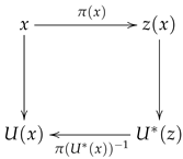
A schematic illustrating this process for the first two steps is shown in Figure 2. For this discrete experiment it is understood that N has to be sufficiently big in order to approximate $n_i^{\left(k\right)}$ for larger step numbers k as the expectation value of the average number of counts in each interval.

In order to prepare for a continuum random process, we consider a density distribution ${\langle {\rho }_n\left(x\right)\rangle }_{N_{\mathsf{\Xi }}}$ at step number n inside of each interval as a result of $N_{\mathsf{\Xi }}$ random events. This density distribution function can be introduced as a continuous function of $x\in [0,1]$

$${\langle {\rho }_n\left(x\right)\rangle }_{N_{\mathsf{\Xi }}}={\displaystyle \frac{1}{\delta x}}\sum _{k=\lfloor x/\delta x\rfloor }^{N_M}{\displaystyle \frac{1}{N_{\xi }\left(k\right)}}\sum _{j=1}^{N_{\xi }\left(k\right)}\theta ({\xi }_j\left(k\right)-x_i)\theta (x_{i+1}-{\xi }_j\left(k\right)),\forall x\in [x_i,x_{i+1}]$$

(7)

where $N_{\mathsf{\Xi }}={\sum }_{k=\lfloor x/\delta x\rfloor }^{N_M}{N}_{\xi }\left(k\right)$ and ${\xi }_j\left(k\right)$ are random numbers drawn from uniform distributions in the intervals ${\xi }_j\left(k\right)\in \mathsf{U}[0,k\delta x]$, $k\ge \lfloor x/\delta x\rfloor$. In a discrete experiment, the number of random experiments, $N_{\xi }\left(k\right)$, performed from each interval k depends on the current population, $n_k^{\left(n\right)}$, inside this interval. For a sufficiently large number of random events $N_{\mathsf{\Xi }}$, we can consider each interval to be populated with the expectation value ${\rho }_n\left(x\right)$ which in the limiting case is given by

$${\rho }_n\left(x\right)\equiv \mathbb{E}\left[{\rho }_n\left(x\right)\right]=\underset{N_{\mathsf{\Xi }}\to \infty }{lim}{\langle {\rho }_n\left(x\right)\rangle }_{N_{\mathsf{\Xi }}}$$

(8)

For the discrete system, it is constant within each interval and it is defined to fulfil a normalisation property

$${\int }_0^{1}dx{\rho }_n\left(x\right)=\sum _{i=1}^M{\int }_{x_{i-1}}^{x_i}dx{\rho }_n\left(x\right)=1$$

(9)

Since the random process only redistributes the density towards the origin, there is a conservation of mass, so that the normalisation property holds for arbitrary $n\ge 0$.

Continuing the random process with a uniform probability distribution from each individual interval will lead to an ongoing shift in the density towards the origin. If an $ϵ$-region is defined as an integer number of intervals, it is understood that in each step there will be new arrivals within this region, and finally, for $n\to \infty$, the whole population will be located inside the $ϵ$-interval.

The change in density in the intervals can be described formally by a propagator; changing the density at position x at step n to a different density at step $n+1$, and therefore the total population, in each interval will be given by

$${\rho }_{n+1}\left(x\right)=\mathcal{P}{\{{\rho }_n;\delta x\}}_x^1$$

(10)

where $\mathcal{P}{\{{\rho }_n;\delta x\}}_x^1$ is a discrete propagator operating on the space discretised by $\delta x$ and collecting all contributions from location x to 1. It propagates the current density distribution within each interval $[x_{i-1},x_i]$ ($i\in [1,M]$) at time step n to time step $n+1$ according to the underlying stochastic process and can be defined as

$$\mathcal{P}{\{{\rho }_n;\delta x\}}_x^1=\sum _{i=\lfloor x/\delta x\rfloor }^{M-1}{\int }_{x_i}^{x_{i+1}}dz{\rho }_n\left(z\right)p\left(z\right)$$

(11)

If we consider the initial step, the density is a $\delta$-function distribution at $x=1$. From there, the probability to jump to any location within the interval $[0,1]$ is 1, i.e., any jump of a random particle, starting at $x=1$ will be located within $[0,1]$. For the general case of a particle being located at $z\in [0,1]$, the probability to jump to location $x<z$ is

$$p(x,z)dz={\displaystyle \frac{dz}{z}}\equiv p\left(z\right)dz$$

(12)

and the density distribution after the first random step can be described as

$${\rho }_1\left(x\right)=\sum _{i=\lfloor x/\delta x\rfloor }^M{\int }_{x_{i-1}}^{x_i}dz{\rho }_0\left(z\right)p\left(z\right)$$

(13)

$$=\sum _{i=I\left(x\right)}^M{\displaystyle \frac{1}{\delta x}}{\int }_{x_{i-1}}^{x_i}dz{\displaystyle \frac{\delta (1-z)}{z}}$$

(14)

$$=1$$

(15)

where we have introduced the notation $I\left(x\right)=\lfloor x/\delta x\rfloor$ to indicate the left index of the interval, in which a particle at x is located. At step n, the density will be given by

$${\rho }_n\left(x\right)=\sum _{i=I\left(x\right)}^M{\int }_{x_{i-1}}^{x_i}dz{\rho }_{n-1}\left(z\right)p\left(z\right)$$

(16)

If we formally consider the limit of $\delta x\to 0$, the integral part gets

$$\underset{\delta x\to 0}{lim}{\int }_{x_i-\delta x}^{x_i}dz{\rho }_n\left(z\right)p\left(z\right)=\delta x{\rho }_n\left(x\right)p\left(x\right)$$

(17)

From Equations (16) and (17) the sum is rewritten as the Riemann integral

$$\underset{\delta x\to 0}{lim}\sum _{i=I\left(x\right)}^M\delta xf\left(x_i\right)={\int }_x^{1}dzf\left(z\right)$$

(18)

so that the combined transition for $\delta x\to 0$ is written as

$${\rho }_n\left(x\right)={\int }_x^{1}dz{\rho }_{n-1}\left(z\right)p\left(z\right)$$

(19)

For the process, which we consider, the probability density is given by $p\left(x\right)=1/x$. That is for each interval $[0,x]$, the total probability to jump from x to any other location $z\in [0,x]$ is $P_{0\to x}={\int }_0^{x}dzp\left(z\right)=1$. Therefore we can write

$${\rho }_n\left(x\right)={\int }_x^{1}dz{\displaystyle \frac{{\rho }_{n-1}\left(z\right)}{z}}$$

(20)

In the initial step the process starts at $x_0=1$ so that the density is written as ${\rho }_0\left(x\right)=\delta (1-x)$. To illustrate the solutions, we write down the first four terms explicitly:

$${\rho }_1\left(x\right)={\int }_x^{1}dz{\displaystyle \frac{{\rho }_0\left(z\right)}{z}}={\int }_x^{1}dz{\displaystyle \frac{\delta (1-z)}{z}}=1$$

(21)

$${\rho }_2\left(x\right)={\int }_x^{1}dz{\displaystyle \frac{{\rho }_1\left(z\right)}{z}}={\int }_x^{1}dz{\displaystyle \frac{1}{z}}=-log\left(x\right)$$

(22)

$${\rho }_3\left(x\right)={\int }_x^{1}dz{\displaystyle \frac{{\rho }_2\left(z\right)}{z}}=-{\int }_x^{1}dz{\displaystyle \frac{log\left(z\right)}{z}}={\displaystyle \frac{1}{2}}log{\left(x\right)}^2$$

(23)

$${\rho }_4\left(x\right)={\int }_x^{1}dz{\displaystyle \frac{{\rho }_3\left(z\right)}{z}}={\displaystyle \frac{1}{2}}{\int }_x^{1}dz{\displaystyle \frac{log{\left(z\right)}^2}{z}}=-{\displaystyle \frac{1}{6}}log{\left(x\right)}^3$$

(24)

From the recursive scheme, Equation (20), we can write down an analytic solution for the time evolution of the density field. Since $p\left(z\right)=1/z$ is given and the density ${\rho }_{n+1}\left(x\right)$ produces, as a result of integration, powers of n of the logarithm, we first evaluate

$${\int }_x^{1}dz{\displaystyle \frac{log{\left(z\right)}^n}{z}}={\displaystyle \frac{{(-1)}^{n+1}}{n+1}}log{\left(x\right)}^{n+1}$$

(25)

from where we get in combination with Equations (21)–(24)

$${\rho }_{n+1}\left(x\right)={\displaystyle \frac{{(-1)}^n}{n!}}log{\left(x\right)}^n\mathrm{or}{\rho }_n\left(x\right)={\displaystyle \frac{{(-1)}^{n-1}}{(n-1)!}}log{\left(x\right)}^{n-1}$$

(26)

Results for the density distribution function are shown in Figure 3 for analytical and numerical values from random walk simulations.

The distribution function for the number of steps to reach the target within the $ϵ$-region is then given as the collection of individual probabilities for n steps and constant distance $x=ϵ<1$, i.e.,

$$p(n+1;ϵ)={\displaystyle \frac{{(-1)}^n}{n!}}{\displaystyle \frac{log{\left(ϵ\right)}^n}{{\sum }_{k=0}^{\infty }\frac{{(-1)}^k}{k!}log{\left(ϵ\right)}^k}}$$

(27)

$$={\displaystyle \frac{{(-1)}^n}{n!}}{\displaystyle \frac{log{\left(ϵ\right)}^n}{e^{|log(ϵ\left)\right|}}}$$

(28)

$$={\displaystyle \frac{1}{n!}}{|log\left(ϵ\right)|}^n{e}^{-|log(ϵ\left)\right|}$$

(29)

or

$$p(n;ϵ)={\displaystyle \frac{1}{(n-1)!}}ϵ{|log\left(ϵ\right)|}^{n-1}$$

(30)

Results for the probability density distribution function are shown in Figure 4.

The shift in n corresponds to the fact that at least one step is needed to move the random walker to the target, even if $ϵ=1$ (it is always assumed that the walker is not yet inside the $ϵ$-region in the initial state). This looks quite similar to a Poisson distribution function $p(k;\lambda )={\lambda }^k{e}^{-\lambda }/k!$, where k is usually a number of occurrences. The present case corresponds to a shifted Poisson distribution function, where the probability at step n depends on the $(n-1)$-th step. The Poisson distribution function is very well studied and has, as the expectation value for the number of occurrences, the value $\lambda$. As shown in Appendix A, the expectation value and the variance of the current process is given by

$$\mathbb{E}\left[n;ϵ\right]=1+|log\left(ϵ\right)|$$

(31)

$$\mathsf{Var}\left[n;ϵ\right]=|log\left(ϵ\right)|$$

(32)

We can define a discrete flux into the $ϵ$-region as the spatial integral over the density change per unit step for $x\in [ϵ,1]$, i.e.,

$$j_r(n;ϵ)={\int }_{ϵ}^{1}dx({\rho }_n\left(x\right)-{\rho }_{n+1}\left(x\right))$$

(33)

$$=-{\displaystyle \frac{{(-1)}^n}{n!}}{\int }_{ϵ}^{1}dx\left(nlog{\left(x\right)}^{n-1}+log{\left(x\right)}^n\right)$$

(34)

which corresponds to the density decay in the region $x>ϵ$. Figure 5 shows a surface plot for $j_r(n;ϵ)$ as a function of step index and size of target region, which shows that the step index for the largest rate of change in the system is slowly increasing with reduced $ϵ$. The curves for a fixed $ϵ$ thereby obey the summation rule

$$\sum _{n=0}^{\infty }{j}_r(n;ϵ)=1$$

(35)

reflecting the fact that on the long term, i.e., $n\to \infty$, the whole density in the system will be located inside the target region $ϵ$.

2.2. Number of Rejected Steps

So far, we have considered the density and the probability for accepted random trial moves bringing the minimum search closer to an $ϵ$-region, which is eventually reached after a certain number of steps n. The complete minimisation process would also account for trial steps which lead to a direction of increasing energy and which are consequently rejected (Figure 6). For the present study, these steps are considered as rejected as a result of an acceptance criterion, which only accepts moves leading to lower energies. Therefore, the question is, how many steps in total would be necessary to bring a random walk inside the target $ϵ$-region

The number of average rejections between each accepted step can be computed along the following considerations. Since we assume a finite interval with a monotonously decreasing energy function, one direction from the current position x will lead downhill, while the other direction leads uphill. As mentioned before, uphill moves might be considered but are rejected as a valid stochastic move. Therefore, we can compute simply the number of stochastic attempts until a downhill move is found. If we consider now the whole configuration space, i.e., states with lower and higher energy, then it is understood that while approaching the $ϵ$-region, the number of possibilities to go downhill in energy is decreasing while the available space with higher energy is increasing. If the trial moves are selected from a uniform random number generator, the probability to move downhill will be given by the ratio of lower energy volume, ${\Omega }_{ϵ}$, to total volume, ${\Omega }_S$, and vice versa the ratio of higher energy volume, ${\Omega }_S\setminus {\Omega }_{ϵ}$, to total volume, ${\Omega }_S$, to move uphill in energy. If the current position of the random walker is x, the total probability to generate trial moves with lower/higher coordinate is therefore given as

$$P(z<x)={\int }_{{\Omega }_{ϵ}}dzP(z>x)={\int }_{{\Omega }_S\setminus {\Omega }_{ϵ}}dz$$

(36)

For the one-dimensional system defined in $[0,1]$, considered here, the probabilities are, therefore, simply the length of regions smaller and larger than x, i.e.,

$$P(z<x)=xP(z>x)=1-x$$

(37)

Therefore, the ratio between uphill and downhill steps is then given by the ratio of the probabilities. For each random walker, the number of rejected uphill steps with respect to an accepted downhill step is then $P(z>x)/P(z<x)=(1-x)/x$. Therefore, if the probability in step n to find a random walker in the interval $dx$ is given by the density ${\rho }_n\left(x\right)$, the ratio between the number of rejections to acceptances is given by the integral over the density multiplied by $P(z>x)/P(z<x)$, i.e.,

$$n_{rej}(n;ϵ)={\int }_{ϵ}^{1}dx{\rho }_n\left(x\right)\left({\displaystyle \frac{1}{x}}-1\right)$$

(38)

$$\begin{array}{cc}\hfill =& {\displaystyle \frac{{(-1)}^{(n-1)}{(-log\left(ϵ\right))}^{n-1}}{(n+1)!}}((n+1)(ϵ-1)\hfill \\ & +\sqrt{ϵ}{(-log\left(ϵ\right))}^{-n/2}{W}_{n/2,(n+1)/2}(-log\left(ϵ\right)))\hfill \end{array}$$

(39)

where $W_{k,l}\left(x\right)$ is the WhittakerM-function [53,54]. Equation (39) means that after n accepted trial moves in a stochastic optimisation procedure with the size of the target region $ϵ$, one will observe on average $n_{rej}(n;ϵ)$ rejected steps before succeeding in a $(n+1)th$ successful move. Since the total integral over the density in the limits $[0,1]$ is constant (conservation of mass), the portion of particles reaching the region $ϵ$ is growing with n and so the total number of rejected particles is decreasing with n. 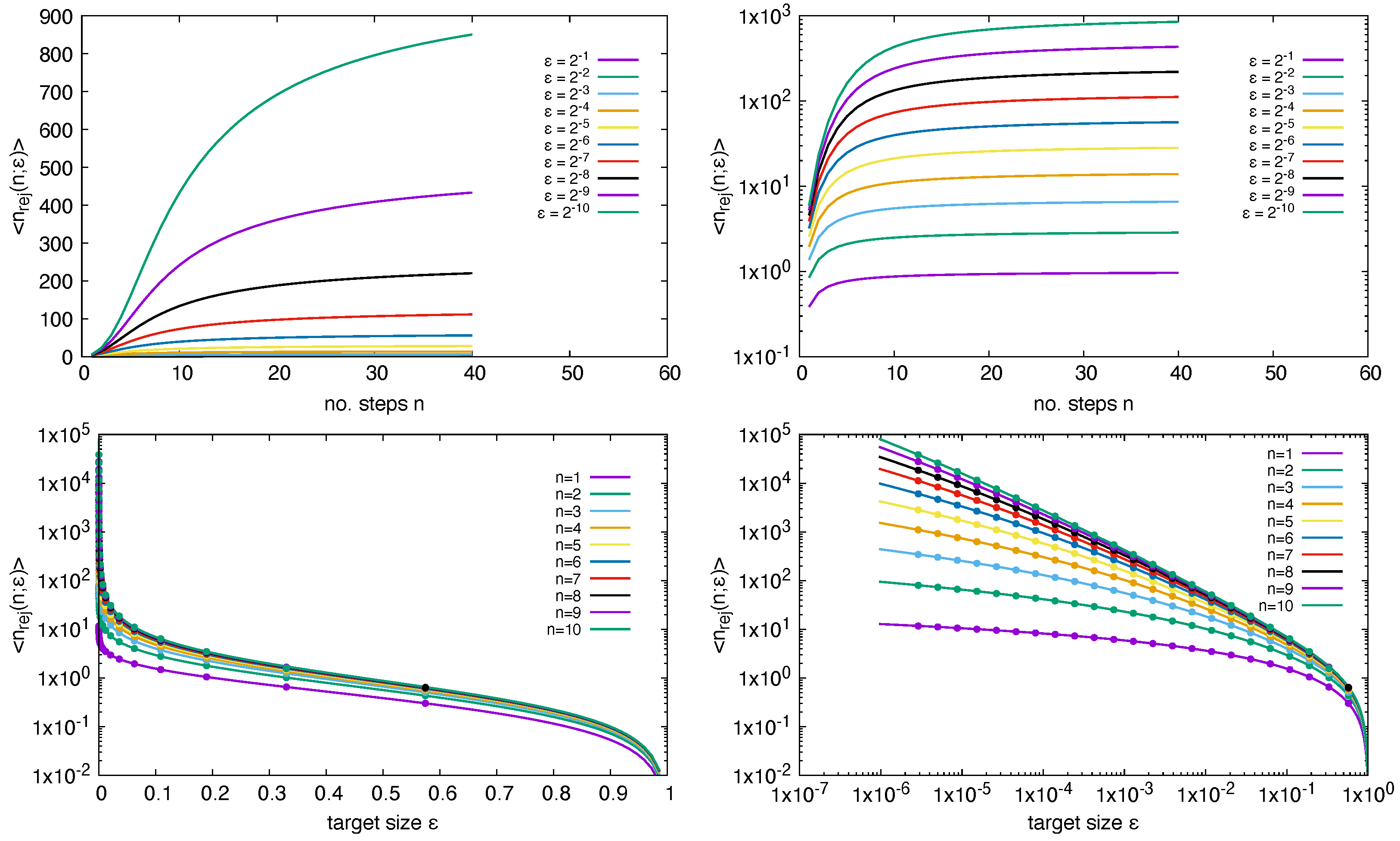In the long run, it is ${lim}_{n\to \infty }\rho (x>ϵ)=0$ and consequently also the number of rejected steps vanishes. Results for Equation (39) are shown in Figure 7. Note that Equation (39) only provides information about the waiting times, i.e., the average number of trial moves between two accepted steps. Therefore, the expectation number of total rejected steps for a random walker until it reaches the target of size $ϵ$ is given by the sum, i.e., the cumulative function

$$\mathbb{E}\left[n_{rej}(n;ϵ)\right]=\sum _{k=1}^n{n}_{rej}(k;ϵ)$$

(40)

or, if the total number of rejections is required for a random walker which tries to find a minimum region of size $ϵ$

$$\mathbb{E}\left[n_{rej}\left(ϵ\right)\right]=\sum _{k=1}^{\infty }{n}_{rej}(k;ϵ)$$

(41)

This is different if we consider the rejections for those particles which are still active in the random walk, i.e., all particles at positions $x>ϵ$. This can be computed if we renormalise the density to 1 within the interval $[ϵ,1]$, i.e.,

$${\widehat{n}}_{rej}^{\left(0\right)}(n;ϵ)={\displaystyle \frac{1}{Q_{ϵ}^{\left(0\right)}\left(n\right)}}{\int }_{ϵ}^{1}dx{\rho }_n\left(x\right)\left({\displaystyle \frac{1}{x}}-1\right)$$

(42)

with

$$Q_{ϵ}^{\left(0\right)}\left(n\right)={\int }_{ϵ}^{1}dx{\rho }_n\left(x\right)$$

(43)

$$\begin{array}{c}={\displaystyle \frac{\sqrt{ϵ}{(-log\left(ϵ\right))}^n}{(n+1)!}}[\sqrt{ϵ}(n+1)\\ +{(-log\left(ϵ\right))}^{-n/2}{W}_{n/2,(n+1)/2}(-log\left(ϵ\right))]\end{array}$$

(44)

where we have used the upper index notation “$\left(0\right)$” to indicate that the underlying probability distribution function is a uniform distribution function. Results are shown in Figure 8 for both Equation (42) and numerical random walk simulations. The number of rejected steps is increasing with the number of step size, since the event space which is available for rejected states, i.e., going uphill in the RW, is increasing. Since the number of active particles in the RW is decreasing in each step, the RW is finally finishing.

2.3. Triangular Distribution Function

With the formalism derived in the last section, we can now also study different underlying distribution functions for the stochastic process. The simplest extension from the uniform distribution function is the triangular distribution, i.e., a B-Spline of order-1. This distribution function can also be considered as the resulting distribution of the sum of two uniformly distributed random variates. To compute the successful trial step distributions, we consider the direction with decreasing step size, i.e., we only consider the positive branch of a centred distribution and write

$${\xi }^{\left(1\right)}=|{\xi }_1^{\left(0\right)}+{\xi }_2^{\left(0\right)}-2{\mu }_0|$$

(45)

In analogy to the case of the uniform distribution, we can write

$${\rho }_1^{\left(1\right)}\left(x\right)={\int }_x^{1}dz{\rho }_0^{\left(1\right)}\left(z\right)p^{\left(1\right)}(x;z)=2{\int }_x^{1}dz{\displaystyle \frac{x\delta (1-z)}{z^2}}=2x$$

(46)

$${\rho }_2^{\left(1\right)}\left(x\right)={\int }_x^{1}dz{\rho }_1^{\left(1\right)}\left(z\right)p^{\left(1\right)}(x;z)=4{\int }_x^{1}dz{\displaystyle \frac{x}{z}}=-4xlog\left(x\right)$$

(47)

$${\rho }_3^{\left(1\right)}\left(x\right)={\int }_x^{1}dz{\rho }_2^{\left(1\right)}\left(z\right)p^{\left(1\right)}(x;z)=-8{\int }_x^{1}dz{\displaystyle \frac{xlog\left(z\right)}{z}}=4xlog{\left(x\right)}^2$$

(48)

$${\rho }_4^{\left(1\right)}\left(x\right)={\int }_x^{1}dz{\rho }_3^{\left(1\right)}\left(z\right)p^{\left(1\right)}(x;z)=8{\int }_x^{1}dz{\displaystyle \frac{xlog{\left(z\right)}^2}{z}}=-{\displaystyle \frac{8}{3}}xlog{\left(x\right)}^3$$

(49)

where we have used the fact that the probability distribution for a forward move is now

$$p^{\left(1\right)}(x;z)=2x/z^2$$

(50)

The meaning is that x is the position, which collects contributions from random walk processes, starting from $z>x$. For a position at z, the total density ${\rho }_n^{\left(1\right)}\left(z\right)$ is moved towards positions $x<z$ with a linear probability function. Since it is considered that the total amount at z is moved, the total probability is normalised to 1, which results in Equation (50). Constructing a recursive scheme from these terms and from the formalism, which was derived, the probability to be located at x after n steps is found to be

$${\rho }_n^{\left(1\right)}\left(x\right)={(-1)}^{n-1}{\displaystyle \frac{2^n}{(n-1)!}}xlog{\left(x\right)}^{n-1}n\in {\mathbb{N}}^{+}$$

(51)

A comparison between results from Equation (51) and a numerical experiment are compared in Figure 9.

The probability distribution, to be located at a position x after n steps, is then readily found to be

$$p(n;x)={\displaystyle \frac{{\rho }_n^{\left(1\right)}\left(x\right)}{{\sum }_{k=1}^{\infty }{\rho }_n^{\left(1\right)}\left(x\right)}}$$

(52)

$$={\displaystyle \frac{2^n}{(n-1)!}}{\displaystyle \frac{{(-1)}^{n-1}xlog{\left(x\right)}^{n-1}}{{\sum }_{k=1}^{\infty }{(-1)}^{n-1}\frac{2^n}{(n-1)!}xlog{\left(x\right)}^{n-1}}}$$

(53)

$$={\displaystyle \frac{2^{n-1}}{(n-1)!}}{(-1)}^{n-1}{x}^{2}log{\left(x\right)}^{n-1}$$

(54)

with mean value and variance (cmp. Appendix A)

$$\mathbb{E}\left[n;ϵ\right]=1-2log\left(ϵ\right)$$

(55)

$$\mathsf{Var}\left[n;ϵ\right]=-2log\left(ϵ\right)$$

(56)

The number of random walk steps, which are rejected as a result of moving upwards in the energy landscape, can be computed in analogy to Equation (38). The number of steps is then found to be

$$n_{rej}^{\left(1\right)}(n;ϵ)={\int }_{ϵ}^{1}dx{\rho }_n\left(x\right)\left({\displaystyle \frac{1}{x^2}}-1\right)$$

(57)

$$={\int }_{ϵ}^{1}dx{\displaystyle \frac{{(-1)}^{n-1}{2}^{n}xlog{\left(x\right)}^{n-1}}{(n-1)!}}\left({\displaystyle \frac{1}{x^2}}-1\right)$$

(58)

$$\begin{array}{c} ={\displaystyle \frac{{(-1)}^{2n+1}x}{(n+1)!}}(2^{n/2}{(-log\left(x\right))}^{n/2}{W}_{n/2,(n+1)/2}(-2log\left(x\right))\\ +{(-2)}^{n}x(n+1){(-log\left(x\right))}^n)\end{array}$$

(59)

where $W_{n/2,(n+1)/2}(-log\left(x\right))$ is again the Whittaker function [53,54]. The first explicitly computed terms for $n_{rej}^{\left(1\right)}(n;ϵ)$ are given in Appendix D. This provides the total number of rejected steps if the random walk has reached n successful downhill steps, i.e., particles which have already reached the target region would contribute with zero unsuccessful uphill steps. If we ask how many steps are performed by those articles which are still active in the random walk, this can be computed by a normalised density within the active region, i.e.,

$${\widehat{n}}_{rej}^{\left(1\right)}(n;ϵ)={\displaystyle \frac{1}{Q_{ϵ}^{\left(1\right)}\left(n\right)}}{\int }_{ϵ}^{1}dx{\rho }_n\left(x\right)\left({\displaystyle \frac{1}{x}}-1\right)$$

(60)

where the normalisation factor, i.e., the integral over the density in the range of $x\in [ϵ,1]$ is given by

$$\begin{array}{cc}\hfill Q_{ϵ}^{\left(1\right)}\left(n\right)& ={\int }_{ϵ}^{1}dx{\rho }_n\left(x\right)\hfill \\ \hfill & ={\displaystyle \frac{ϵ{(-2log\left(ϵ\right))}^n}{(n+1)!}}[ϵ(n+1)\hfill \end{array}$$

(61)

$$+{(-2log\left(ϵ\right))}^{-n/2}{W}_{n/2,(n+1)/2}(-2log\left(x\right))]$$

(62)

2.4. Polynomial Distributions of Order-k

Applying the same technique to compute densities as before, we write

$${\rho }_n^{\left(k\right)}\left(x\right)={\int }_x^{1}dz{\rho }_{n-1}^{\left(k\right)}\left(z\right)p^{\left(k\right)}(z;x)$$

(63)

$$={\int }_x^{1}dz(k+1){\rho }_{n-1}^{\left(k\right)}\left(z\right){\displaystyle \frac{x^k}{z^{k+1}}}$$

(64)

$$={\displaystyle \frac{1}{(n-1)!}}{x}^k{(k+1)}^n{(-1)}^{n-1}log{\left(x\right)}^{n-1}$$

(65)

where the upper index $\left(k\right)$ indicates the polynomial order, i.e., $k\in \mathbb{N}$ and we have used the normalised polynomial distribution function (cmp. Equation (50))

$$p^{\left(k\right)}(z;x)=(k+1){\displaystyle \frac{x^k}{z^{k+1}}}$$

(66)

Due to the conservation of total probability to find a random walker in the interval $x\in [0,1]$, it is ${\int }_0^{1}dx{\rho }_n^{\left(k\right)}\left(x\right)=1,\forall n,k\in \mathbb{N}$.

The probability distribution to hit the target after n steps is given by the sum over all densities for a given target size $ϵ$ and normalised to 1. Therefore

$$p^{\left(k\right)}(n;ϵ)={\displaystyle \frac{{\rho }_n^{\left(k\right)}(x;ϵ)}{{\sum }_{n=1}^{\infty }{\rho }_n^{\left(k\right)}(x;ϵ)}}$$

(67)

It is found that ${\sum }_{n=1}^{\infty }{\rho }_n^{\left(k\right)}(x;ϵ)=(k+1)/x$, so that

$$p^{\left(k\right)}(n;ϵ)={\displaystyle \frac{1}{(n-1)!}}{(-1)}^{n-1}{(k+1)}^{n-1}{x}^{k+1}log{\left(x\right)}^{n-1}$$

(68)

Results for Equation (68) for the case of a triangular distribution function are shown in Figure 10.

It is readily found that the normalisation condition of this probability distribution holds. The first moments of n are found to be (cmp. Appendix A)

$${\mu }_0^{\left(k\right)}\left(ϵ\right)=\sum _{n=1}^{\infty }{p}^{\left(k\right)}(n;ϵ)=1$$

(69)

$${\mu }_1^{\left(k\right)}\left(ϵ\right)=\sum _{n=1}^{\infty }n{p}^{\left(k\right)}(n;ϵ)=1-(k+1)log\left(ϵ\right)$$

(70)

$${\mu }_2^{\left(k\right)}\left(ϵ\right)=\sum _{n=1}^{\infty }{n}^2{p}^{\left(k\right)}(n;ϵ)=1-3(k+1)log\left(ϵ\right)+{(k+1)}^{2}log{\left(ϵ\right)}^2$$

(71)

from where the expectation value and variance is given as

$$\mathbb{E}\left[n;ϵ\right]=1-(k+1)log\left(ϵ\right)$$

(72)

$$\mathsf{Var}\left[n;ϵ\right]=-(k+1)log\left(ϵ\right)$$

(73)

A comparison between analytical and numerical results of Equation (72) is shown in Figure 11.

As for the uniform random process, we compute the number of rejected steps before encountering the next successful step as

$$\begin{array}{cc}\hfill n_{rej}^{\left(k\right)}(n;ϵ)& ={\int }_{ϵ}^{1}dx{\rho }_n^{\left(k\right)}(x;ϵ)\left({\displaystyle \frac{1}{x}}-1\right)\hfill \\ \hfill & =-{\displaystyle \frac{{(k+1)}^n}{(n+1)!}}[{ϵ}^k(ϵ-1)(n+1){(-log\left(ϵ\right))}^n\hfill \end{array}$$

(74)

$$\begin{array}{c}+W\left({\displaystyle \frac{n}{2}},{\displaystyle \frac{n+1}{2}},-(k+1)log\left(ϵ\right)\right){ϵ}^{(k+1)/2}{\left(-{\displaystyle \frac{1}{k+1}}log\left(ϵ\right)\right)}^{n/2}\hfill \\ -W\left({\displaystyle \frac{n}{2}},{\displaystyle \frac{n+1}{2}},-klog\left(ϵ\right)\right){ϵ}^{k/2}{\left(-{\displaystyle \frac{1}{k}}log\left(ϵ\right)\right)}^{n/2}]\hfill \end{array}$$

(75)

In this expression the integral is carried out over the density in the interval $x\in [ϵ,1]$, i.e., it does only correspond to random walkers which are not yet finished and therefore, with increasing step number n, the number of rejections, $n_{rej}^{\left(k\right)}(n;ϵ)$, will finally decrease—to zero. Starting with N random walkers will therefore lead to the total number of waiting steps, which are accumulated in the experiment. Results are shown in Figure 12 for analytical results from Equation (75) and numerical values. The number of rejected steps is increasing with the number of step size, since the event space which is available for rejected states, i.e., going uphill in the RW, is increasing. Since the number of active particles in the RW is decreasing in each step, the RW is finally finishing.

To consider the average waiting time for individual random walkers, which have not yet reached the target region, i.e., those which are still active, we compute the normalised step number by

$${\widehat{n}}_{rej}^{\left(k\right)}(n;ϵ)={\displaystyle \frac{1}{Q_{ϵ}^{\left(k\right)}}}{n}_{rej}^{\left(k\right)}(n;ϵ)$$

(76)

which takes into account a normalised density distribution outside the target region. The normalisation factor $Q_{ϵ}^{\left(k\right)}$ is readily found as

$$\begin{array}{ccc}\hfill Q_{ϵ}^{\left(k\right)}& =& {\int }_{ϵ}^{1}dx{\rho }_n^{\left(k\right)}(x;ϵ)\hfill \\ & =& -{\displaystyle \frac{log\left(ϵ\right)}{(n+1)!}}[(n+1){(k+1)}^n{ϵ}^{(k+1)}(-log{\left(ϵ\right)}^{n-1})\hfill \\ & & +{(k+1)}^{n/2}{ϵ}^{(k+1)/2}(-log{\left(ϵ\right)}^{n/2-1})W\left({\displaystyle \frac{n}{2}},{\displaystyle \frac{n+1}{2}},-(k+1)log\left(ϵ\right)\right)]\hfill \end{array}$$

(77)

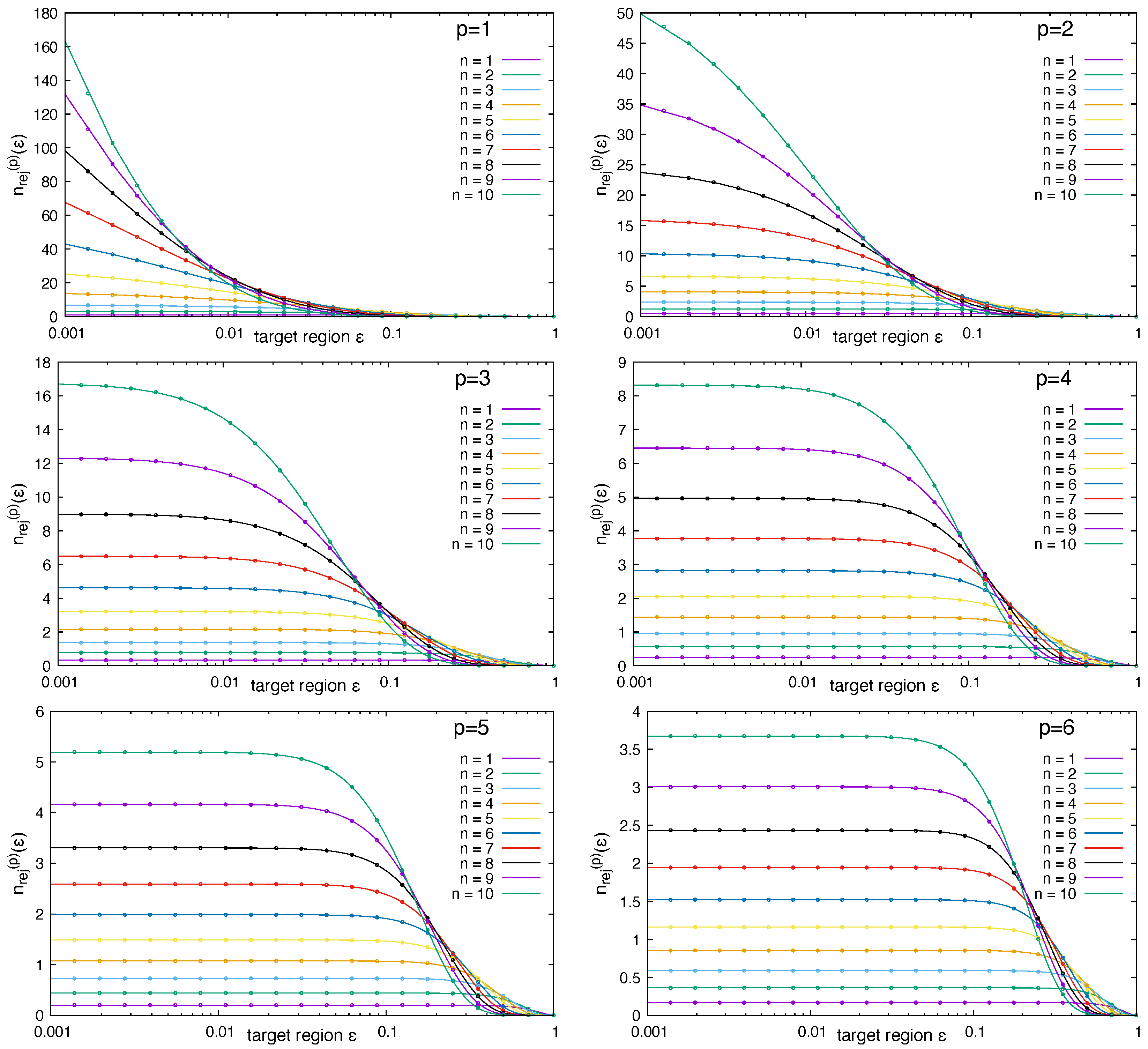
Results for Equation (76) are presented in Figure 13 for polynomial distribution functions of order $p=[1,6]$. The number of rejected steps is increasing with number of step size, since the event space which is available for rejected states, i.e., going uphill in the RW, is increasing. Since the number of active particles in the RW is decreasing in each step, the RW is finally finishing. In Figure 14 we further compare the number of rejected trial moves as function of the number of steps in the random walk.

2.5. The Case of Non-Monotonous Objective Functions

For this case there is no simple way to make an analytical prescription of the density distribution, since regions in space may contain local minima and the resulting density, $\rho (x,n)$, is not simply the integral over a known region of space, from where contributions are gathered. Each point in space, x, is related to an energy, $U\left(x\right)$, but the set of coordinates, i.e., spatial regions for which $U\left(x^{\prime }\right)<U\left(x\right)$, might not be simply connected, but separated by energy barriers. Therefore, there is no straightforward way to find the whole set of coordinates $\left\{x^{\prime }\right|(U\left(x^{\prime }\right)<U\left(x\right))\}$. In order to perform a convergence analysis we consider a transformed function. The basic idea is to use the concept of decreasing rearrangement [48,49,50]. To make this concept more clear, we assume that the function of interest, $f\left(x\right)$, is measurable and we can introduce a distribution function $\tilde{n}\left(x\right)=m\left\{\right|f|>x\}$, where $m(.)$ denotes the measure. Then the rearrangement $f^{*}$ of function f is defined as

$$f^{*}\left(x\right)=inf\{z\ge 0,\tilde{n}\left(z\right)\le x\}$$

(78)

The function $f^{*}\left(x\right)$ accordingly contains all values of the original function $f\left(x\right)$ but in an ordered way, so that the function is monotonously decreasing. Specifically, the computation of powers of that function holds

$${\int }_0^{\infty }{dx\left|f\left(x\right)\right|}^p={\int }_0^{\infty }dx{\left|f^{*}\left(x\right)\right|}^p$$

(79)

In that way we again consider a monotonously decaying energy function in the transformed space, for which the same principles apply which we found before. Practically we introduce a discretisation in space, $x_i$, for the original energy function, where $x_i$ is a coordinate of a node i and the interval width is $\delta x=x_{i+1}-x_i$ with corresponding energies $U_i=U\left(x_i\right)$. If we make the assumption that $U\left(x\right)\in {\mathcal{C}}^1$, the continuous function is obtained via $U\left(x\right)={lim}_{\delta x\to 0}{U}_i\left(x_i\right)\in \mathbb{R}$. Therefore the sorted sequence of energies $U_i^{*}=U^{*}\left(z_i\right)=U\left(x\left(z_i\right)\right)$ are constructed from a permuted series $\left\{z\right\}=\{z_1,\dots ,z_n\}\leftarrow \pi \left(\left\{x\right\}\right)=\pi \left(\{x_1,\dots ,x_n\}\right)$, for which

$$z\in \{z_i,i\in [0,1/\delta x]\}\mathrm{with}{U}^{*}\left(z\right)\in \{U^{*}\left(z_i\right)\le U^{*}\left(z_{i+1}\right),i\in [0,1/\delta x]\}$$

(80)

This can be represented schematically as

In order to apply the same strategy of analysis, which we have considered before, the following procedure is suggested. Since we consider a stochastic experiment, where random variates are generated on the entire interval $x\in [0,1]$ and trial moves are only accepted when a lower energy state is found, we can reformulate the set up of the experiment in the following way: we consider a sorted energy function in such a way that a transformation $z_i=z\left(U\left(x_j\right)\right)$ is performed, which guarantees that

$$U^{*}\left(z_i\right)-U^{*}\left(z_i^{\prime }\right)\ge 0z_i<z_i^{\prime }$$

(81)

To compare with the numerical values, we apply a similar procedure as in the stochastic experiment, i.e., we sum all contributions inside an interval $\delta x$ and assign the result to the next upper integer interval index. For the analytical result this implies performing an integral inside the interval $[x,x+\delta x]$, which allows a direct comparison. For the analytical result, Equation (26), it therefore follows

$${\rho }_k^{*}\left(n\right)={\displaystyle \frac{1}{\delta x}}{\int }_{(k-1)\delta x}^{k\delta x}dz{\rho }_n^{*}(z;ϵ)$$

(82)

$$={\displaystyle \frac{1}{\delta x}}{\int }_{(k-1)\delta x}^{k\delta x}dz{\displaystyle \frac{{(-1)}^{n-1}}{(n-1)!}}log{\left(z\right)}^{n-1}$$

(83)

$$=\left\{\begin{array}{ccc}1\hfill & :& n=0\hfill \\ {\displaystyle (n-1)!\frac{z}{\delta x}[\frac{{log}^{(n-1)}\left(z\right)}{(n-1)!}}\hfill \\ {\displaystyle +\sum _{m=1}^{n-2}\frac{{(-1)}^{n-1-m}}{m!}{log}^m\left(z\right)+{(-1)}^m]{|}_{(k-1)\delta x}^{k\delta x}}\hfill & :& n>0\hfill \end{array}\right.$$

(84)

This shows that the concepts, which were presented for the monotonously decaying functions discussed initially, can be transferred one-to-one if we apply the technique of decreasing rearrangement. Practically, this might be not applicable to an arbitrary function, for which the minimum is to be found. However, we see that the analysis then provides a helpful measure to estimate how many steps will be needed on average to decrease the energy value further if a given number of successful steps has already been performed. Therefore, the analysis provides a general framework to judge the effectiveness of stochastic optimisation and shows a kind of worst-case scenario, which can then be put in relation to other, more efficient methods. Therefore, the analysis provides an analytical framework for a bottom-line-model, so that by proper analysis of other optimisation methods, we can quantify how much faster a given method is with respect to simple or blind stochastic optimisation.

2.6. Model Systems

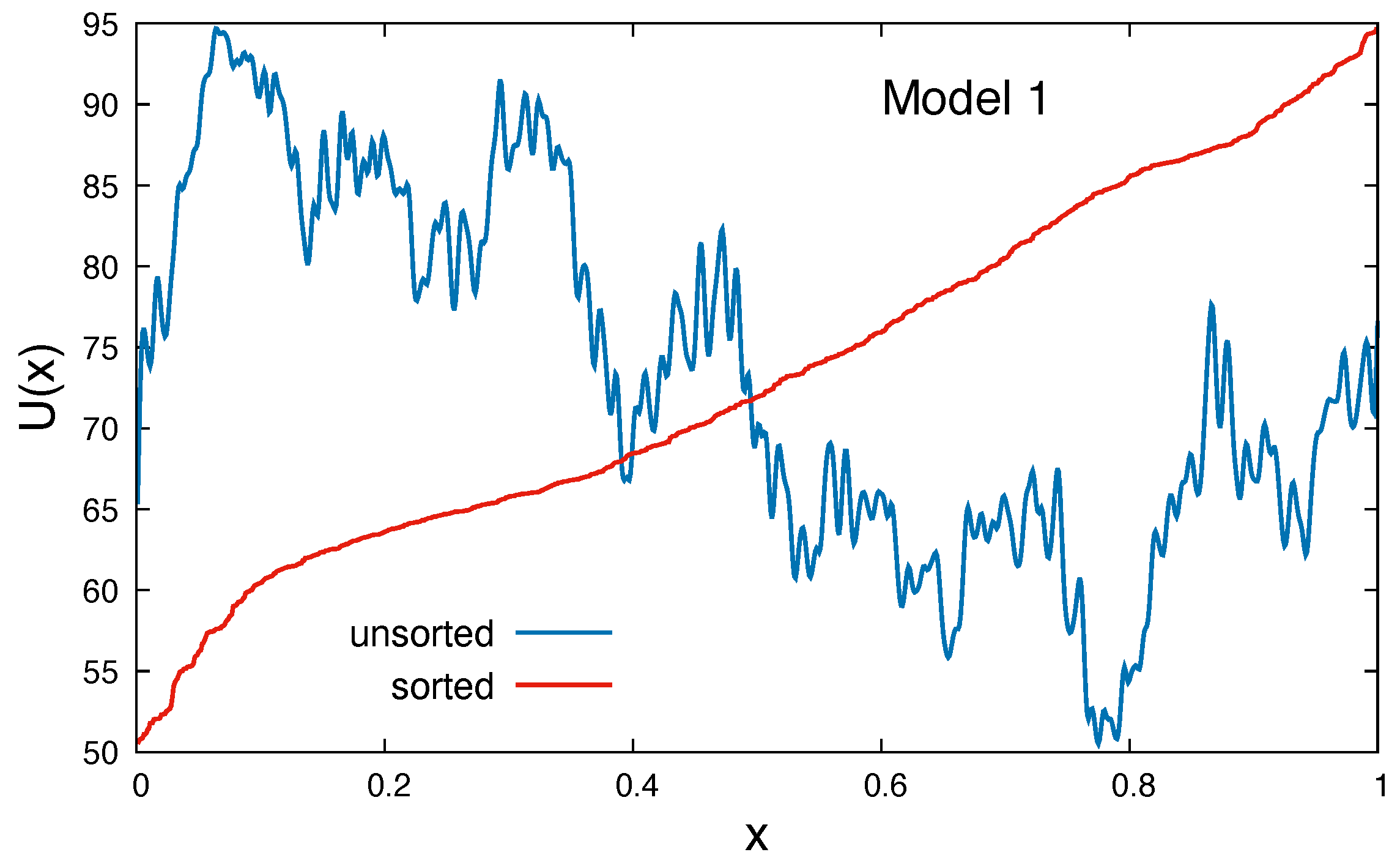
In this section we apply two different non-monotonous functions as the underlying potential surface and perform trial moves to minimise the system energy. As described previously, we use the technique of decreasing rearrangement to demonstrate, numerically and analytically, the applicability of the formalism, Equation (84), developed for the monotonously decaying case. In order to obtain sufficient number of experimental data, a large number ($N={10}^8$) of experiments has been used to exploit the underlying function. Both model systems show a rough structure with many local minima. The simple goal here is to demonstrate that the same formalism, which has been developed for the assumption of monotonously decaying functions can be applied here. In that sense, the global stochastic optimisation approach, which is analysed here, is agnostic with respect to local minima, since each point on the function can be reached with the same probability. Therefore, the technique of decreasing rearrangement can be applied here to demonstrate the convergence behaviour of global stochastic optimisation on rough functions. The experimental setup starts with a uniform density distribution, i.e., the initial position is chosen randomly with a uniform random number generator. If a random move leads to a lower function value, a counter for the experiment is increased by one and the position of the random position is stored in a histogram, corresponding to this counter. Therefore, histograms are constructed for n successful random moves and averaged over all the performed experiments. This leads to an average density distribution, which can be compared with the analytical density description, Equation (84).

2.6.1. Model System 1

The underlying test function, $U\left(x\right)$, is defined as

$$\begin{array}{cc}\hfill U\left(x\right)=& {\displaystyle \sum _{i=1}^{N_1}}{a}_{1,i}cos\left(2\pi {\displaystyle \frac{x-c_{1,i}}{b_{1,i}}}\right)-a_{2,i}sin\left(2\pi {\displaystyle \frac{x-c_{2,i}}{b_{2,i}}}\right)\hfill \\ & +a_{3,i}cos\left(2\pi {\displaystyle \frac{x-c_{3,i}}{b_{3,i}}}\right)\times sin\left(2\pi {\displaystyle \frac{x-c_{4,i}}{b_{4,i}}}\right)\hfill \end{array}$$

(85)

with $N_1=20$. Values for the parameters $a_{k,i},b_{k,i},c_{k,i}$ are given in Appendix F,

Table A1. Parameters $a_{i,k}$ and $b_{i,k}$ for Model System 1.

Index k	${\mathit{a}}_{1,\mathit{k}}$	${\mathit{a}}_{2,\mathit{k}}$	${\mathit{a}}_{3,\mathit{k}}$	${\mathit{b}}_{1,\mathit{k}}$	${\mathit{b}}_{2,\mathit{k}}$	${\mathit{b}}_{3,\mathit{k}}$	${\mathit{b}}_{4,\mathit{k}}$
1	4.390	7.485	7.172	10.501	10.520	6.469	26.330
2	7.562	5.198	7.125	5.699	6.560	17.444	9.216
3	3.560	5.718	6.498	0.196	11.836	25.204	25.299
4	0.348	9.913	20.987	14.443	6.511	23.996	4.783
5	2.701	3.516	14.768	1.068	15.402	22.369	23.881
6	6.436	4.363	11.032	3.718	5.238	19.290	14.675
7	6.366	2.794	11.240	9.437	8.692	4.293	20.627
8	0.950	10.004	3.941	5.471	7.078	32.063	5.442
9	9.331	3.123	10.241	9.219	1.181	0.349	9.100
10	0.793	3.135	4.787	0.044	4.911	1.103	25.434
11	2.726	2.654	3.443	6.444	3.717	36.231	21.825
12	3.563	2.159	9.255	5.203	11.723	11.998	15.442
13	6.456	0.505	12.519	12.686	7.317	22.017	19.387
14	7.638	11.257	1.476	5.383	2.881	34.070	10.467
15	7.807	1.960	9.229	10.998	0.703	37.445	17.563
16	2.794	4.799	20.585	10.644	12.639	14.420	14.609
17	4.875	1.511	3.925	6.252	5.693	4.068	19.079
18	8.359	5.932	7.686	1.407	13.970	32.728	7.608
19	3.259	3.684	2.626	13.292	3.240	14.631	11.557
20	4.522	2.241	3.768	0.131	3.063	11.810	9.459

and

Table A2. Parameters $c_{i,k}$ for Model System 1.

Index k	${\mathit{c}}_{1,\mathit{k}}$	${\mathit{c}}_{2,\mathit{k}}$	${\mathit{c}}_{3,\mathit{k}}$	${\mathit{c}}_{4,\mathit{k}}$
1	19.747	8.464	13.329	3.276
2	3.294	7.085	5.882	10.901
3	5.178	7.872	7.003	7.783
4	21.753	8.916	0.130	5.083
5	21.825	7.214	12.359	3.667
6	14.217	13.327	1.208	6.384
7	20.605	13.681	12.093	6.801
8	11.037	7.927	2.617	3.041
9	8.160	3.556	9.284	4.364
10	10.838	10.837	6.507	3.989
11	0.201	0.217	10.883	11.858
12	18.857	8.278	9.495	3.637
13	20.370	3.550	7.205	7.519
14	6.037	6.987	5.145	14.307
15	10.168	3.974	5.424	8.345
16	15.246	9.316	4.405	8.951
17	4.617	9.981	3.281	4.641
18	15.746	0.094	9.423	11.156
19	0.451	8.705	8.303	0.113
20	5.751	13.332	7.369	2.097

. To smoothen the strength of fluctuations, the function was averaged over 10 cycles via

$$U^{(k+1)}\left(x\right)={\displaystyle \frac{1}{4}}\left(U^{\left(k\right)}(x-\delta x)+2U^{\left(k\right)}\left(x\right)+U^{\left(k\right)}(x+\delta x)\right)$$

(86)

where $k\in [0,9]$ with $U^{\left(0\right)}\left(x\right)=U\left(x\right)$ from Equation (85) The potential function $U\left(x\right)$ and its sorted counterpart $U^{*}\left(x\right)$ are shown in Figure 15.

2.6.2. Model System 2

The underlying test function, $U\left(x\right)$, is defined as

$$U\left(x\right)=-\sum _{k=1}^{N_2}{\displaystyle \frac{a_k}{|x-b_k|+ϵ}}$$

(87)

with $N_2=20$. In order to avoid divergences, the constant term $ϵ={10}^{-8}$ was introduced. Values for the parameters $a_k,b_k$ are listed in Appendix G,

Table A3. Parameters for Model System 2.

Index k	${\mathit{a}}_{\mathit{k}}$	${\mathit{b}}_{\mathit{k}}$
1	0.467	0.218
2	0.632	0.685
3	0.058	0.582
4	0.851	0.119
5	0.165	0.458
6	0.302	0.720
7	0.187	0.872
8	0.543	0.446
9	0.880	0.952
10	0.852	0.845
11	0.215	0.334
12	0.094	0.328
13	0.220	0.294
14	0.900	0.636
15	0.145	0.704
16	0.476	0.012
17	0.414	0.836
18	1.000	0.888
19	0.269	0.830
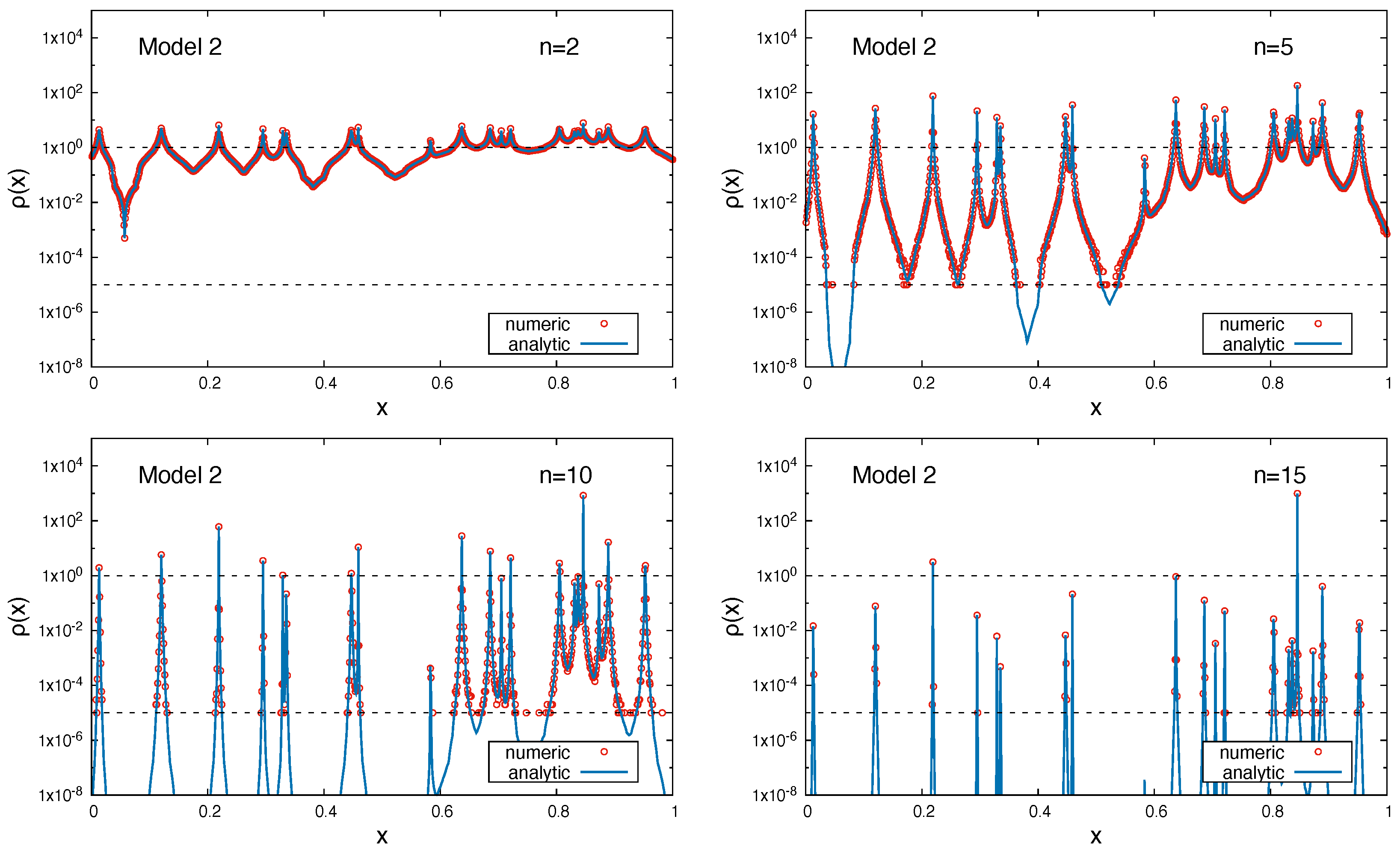
20	0.899	0.804

. The potential function $U\left(x\right)$ and its sorted counterpart $U^{*}\left(x\right)$ are shown in Figure 16. It is to be noted that the plot shows the absolute value of $U\left(x\right)$ on a logarithmic scale, i.e., the highest peak value at $x\approx 0.85$ corresponds to the minimum in the system.

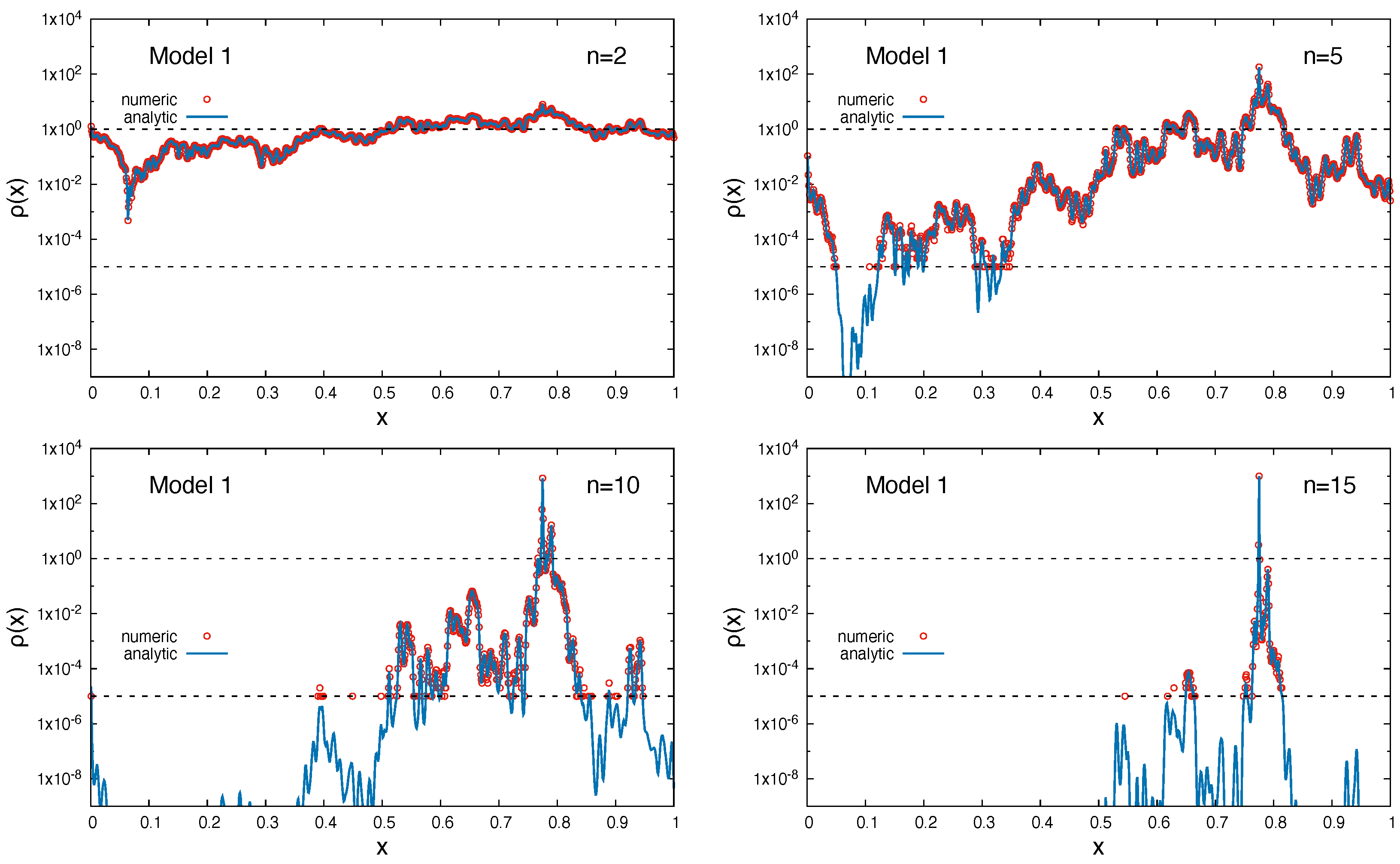
As can be observed for both model systems, the analytical and numerical results perfectly agree within numerical noise for the smallest values in the histogram of Figure 17 and Figure 18. On the one hand, this is due to the limited number of experiments; on the other hand, this is also due to the size of the interval ($\delta x=1\times {10}^{-3}$), which was chosen in order to resolve the sharp peaks in the potential function of model 2. In Figure 17 and Figure 18 the density evolution of the random walkers is shown for different iteration counts. For the model systems 1 and 2, the global minima are found at $x_1\approx 0.78$ and $x_2=0.85$, respectively. It is clearly seen that the density peaks at $x_1$ (Figure 19) and $x_2$ (Figure 20) is increasing for larger iteration counts n, while the rest of the system shows a strongly decreasing density, which is indicative for the assembly of random walkers in the global minimum of the systems. It is again demonstrated that the analytical description of the iteration process is in very close agreement to the numerical experiment, which deviates only due to limited statistics and interval width in the histogram.

2.7. Performance Considerations

From the findings it is possible to derive some performance considerations. Until now the main results which could be obtained were the analytical predictions of the number of both accepted (Equation (31)) and rejected (Equation (41)) steps. If we consider the evaluation time of operations for accepted (${\tau }_{acc}$) and rejected (${\tau }_{rej}$) trial moves, i.e., ${\tau }_{tot}={\tau }_{acc}+{\tau }_{rej}$, we can give an estimate for the overall performance, measured in execution time $T_{rw}$, in terms of $ϵ$. If we denote the expectation values for the number of accepted and rejected steps as $N_{acc}$ and $N_{rej}$ we can write

$$T_{rw}\left(ϵ\right)=N_{acc}\left(ϵ\right){\tau }_{acc}+N_{rej}\left(ϵ\right){\tau }_{rej}$$

(88)

The number of accepted steps has an obvious logarithmic scaling behaviour with $ϵ$. For the rejected steps, we will graphically show in Section 3 a scaling of $N_{rej}\left(ϵ\right)\approx {ϵ}^{-1}$. Therefore, the performance of the random walk optimisation procedure as described in the present article has a complexity of $\mathcal{O}\left({ϵ}^{-1}\right)$. As a motivation, we already anticipate here that the generalisation of the performance to higher dimensions follows a $\mathcal{O}\left({ϵ}^{-d}\right)$ behaviour, where d is the space dimension of the random walker.

3. Outlook for Multi-Dimensional Spaces

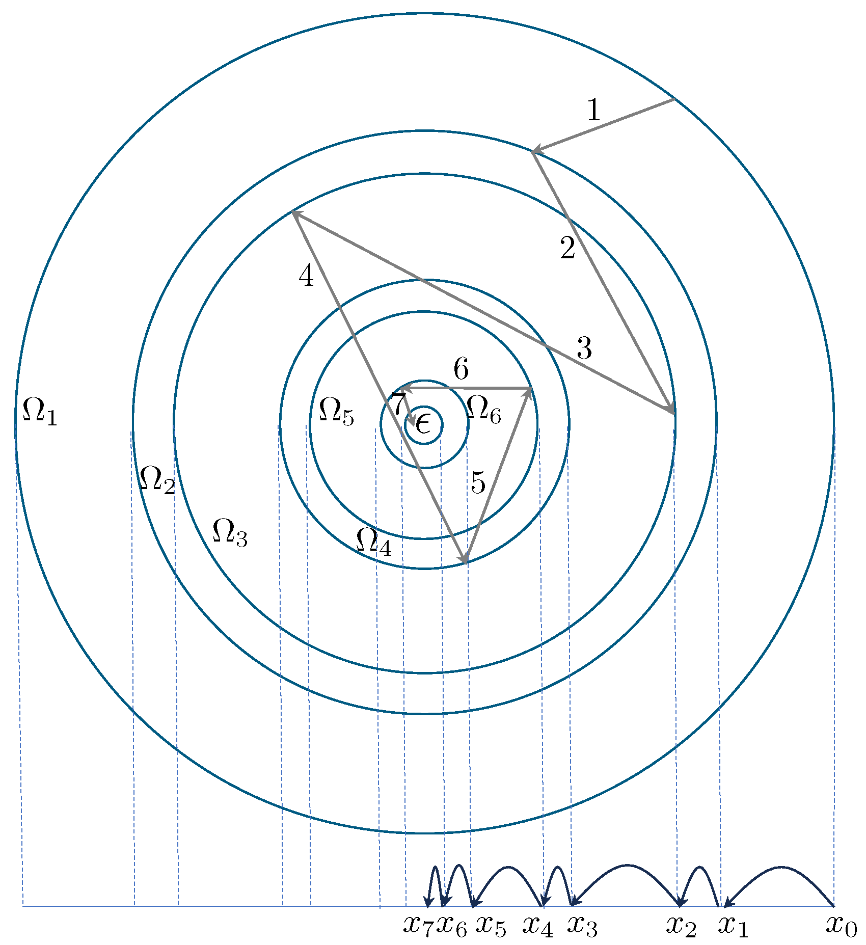
A schematic for a two-dimensional search space is illustrated in Figure 21. This can be easily extended to n-dimensional spaces as n-spheres. Starting from the simple basic idea of a deceasing energy function, the procedure is then similar than for the one-dimensional case, where a walker starts from the boarder of a system and proceeds walking until it reaches an $ϵ$-region, defined around the global minimum in the system. It is understood that the initially placed random point can then be considered to be located on the surface of an n-sphere and that it further proceeds towards the centre of the sphere. From Figure 21 it becomes conceptually clear that search spaces, ${\Omega }_{<}\subseteq \Omega$, can be characterised by isosurfaces, which enclose only smaller values than the value on the boarder, $\partial {\Omega }_{<}$. If the system is spherically symmetric, the only relevant measure is the distance $r^{\left(n\right)}={\parallel {\mathbf{r}}_i^{\left(n\right)}-{\mathbf{r}}_{ϵ}\parallel }_2$, where ${\mathbf{r}}_i^{\left(n\right)}$ is the position of random walker i at iteration step n and ${\mathbf{r}}_{ϵ}$ the minimum location. Therefore, by transforming coordinates to n-dimensional spherical coordinates, it is only the radial variable r which is of relevance for the acceptance of steps and not the angular degrees of freedom. Angular variables can be integrated out, which reduces the problem to a similar problem to the one-dimensional case. For non-monotonous cases the technique of symmetric decreasing rearrangement can be applied here [55,56]. In this case Equation (79) is still fulfilled, so the main properties of the function for the minimisation procedure should be preserved. Although it is not guaranteed that all transformed functions possess the continuity property [55], this should not present a problem for the discussion here, since this was not a requirement for the derived formalism. Therefore, the arguments, which we used for the one-dimensional case, should also be valid for non-homogeneous functions in a n-dimensional space. An issue which was not considered in the present article may occur with constrained-optimisation, including whether constraints can be consistently be transformed from the original to the rearranged function representation.

A major difference between the one-dimensional case and the n-dimensional system becomes more obvious for the number of rejected steps between accepted ones. Qualitatively, a strong increase in rejected steps is expected, which can be understood by the increased number of degrees of freedom in higher dimensions. In Equation (37) the argument was based on the ratio of the volumes between the space which contains smaller values (e.g., energy) and the volume of space with larger values. During the optimisation process, ${\Omega }_{<}$ becomes restricted and shrinks in volume. If a global sampling strategy with a uniform distribution of random numbers in ${\mathbb{R}}^d$ is taken, it follows that the probability for a random walker to move from higher to lower values reduces proportionally to the volume. If we consider L as an average length scale for each dimension of the volume ${\Omega }_{<}$ and set the total volume of the system to $|\Omega |=|{\Omega }_{<}{|+||\Omega |}_{>}|=1$, then, in analogy to Equation (38), the number of rejected steps increases as

$$n_{rej}(n,\mathbf{x}\in \partial {\Omega }_{<})={\displaystyle \frac{1}{|{\Omega }_{<}|}}\propto {\displaystyle \frac{1}{L^d}}$$

(89)

which is a power law relation for the number of rejected steps depending on the dimensionality of the system. For our simulated system we can provide a more precise scaling. If we respect that the system is enclosed by a box ${[-1,1]}^d$, but the restricted motion of a random walk proceeds towards the centre of the box by jumping to surfaces of decreasing d-spheres with volume $V_d\left(r\right)={\pi }^{d/2}{r}^d/\Gamma (d/2+1)$, we get a scaling relation ${\rho }_d\left(r\right)=2^d/V_d\left(r\right)$ of

$${\rho }_d\left(r\right)={\displaystyle \frac{2^d\Gamma (d/2+1)}{{\pi }^{d/2}{r}^d}}$$

(90)

To illustrate this behaviour, numerical experiments were conducted for random samplings in d-dimensional space ${\Omega }_d={[-1,1]}^d$, where a target region ${\Omega }_{ϵ}$ was defined in the centre of the box. Numerical simulations were conducted in the same spirit as for the one-dimensional system, i.e., a random point with coordinate ${\mathbf{x}}_{\mathbf{n}}=\left\{{\mathbf{x}}_i\right|U\left({\mathbf{x}}_{\mathbf{i}}\right)<U\left({\mathbf{x}}_{\mathbf{n}-\mathbf{1}}\right)\}$ was accepted as new minimum value. 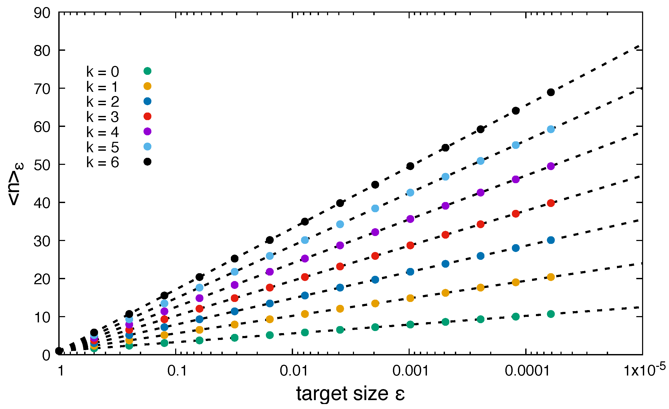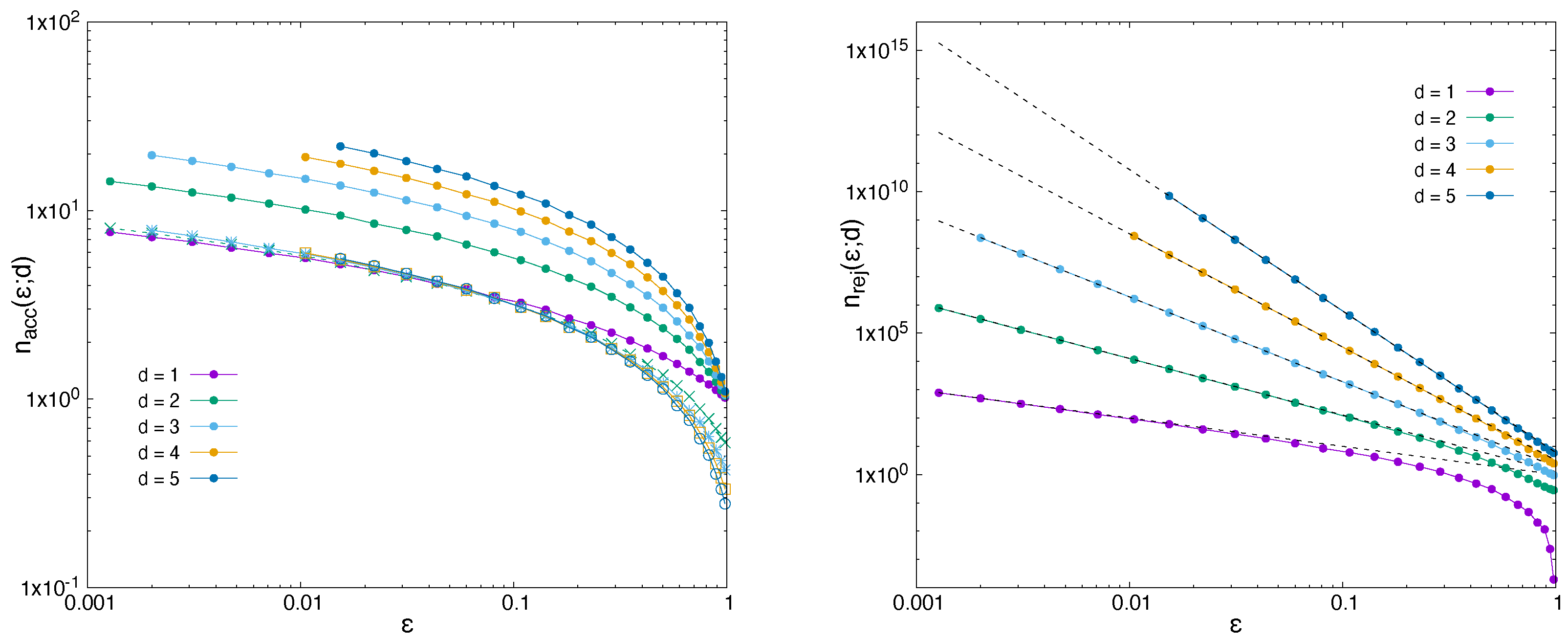Figure 22 shows results for number of steps in dimensions $d=[1,5]$ for both accepted steps (left) and rejected steps (right) as function target size $ϵ$. We stress that these are preliminary results, since a detailed, formal analysis would go beyond the present intention of the work, but it seems obvious that both accepted and rejected steps follow a scaling relation, which is more obvious for the rejected number of steps. As was mentioned before, a simple geometric argument provides the asymptotic scaling for small values of $ϵ$, which can be verified by the superimposed dotted lines. For the accepted steps the transition from an accepted sample to a point in n-space with a smaller energy involves the mean free path from the surface of a n-sphere towards its centre. As a rough measure we computed the mean step size, $\langle \parallel \delta \mathbf{x}{\parallel }_2\rangle$ of a random walker during the minimisation procedure (i.e., mean step size between accepted points $\left\{{\mathbf{x}}_n\right\}$). In the figure, the scaled results for $n_{rej}{(ϵ;d)\langle \parallel \delta \mathbf{x}\parallel }_2\rangle /d$ are superimposed, which show a very similar behaviour for small value of $ϵ$. This shows that the number of steps to reach a region of size $ϵ$ increases as $\mathcal{O}\left(d\right)$, since the mean step size $\langle \parallel \delta \mathbf{x}{\parallel }_2\rangle$ only weakly increases with d (for dimensions $d=[1,5]$ the values of the steps sizes are in value $\{1,1.13,1.2,1.24,1.27\}$). Note that the scaled value for the one-dimensional case is preserved, since $d=1$ and $\langle \delta x\rangle =1$. An in-depth formal discussion for this scaling needs to be performed and will be discussed in a forthcoming work. Here, the intention for the qualitative level of discussion was to provide an outlook for the more general case in higher dimensions.

4. Discussion

We have analysed the process of a stochastic optimisation to find a minimum in a system with monotonously decaying energy function. Although this is a rather simplistic system, it provides interesting insights from the perspective of the stochastic process. If only the successful steps (i.e., accepted steps in the stochastic optimisation process) are considered, one can consider the problem as a random walk with decreasing step size for the case where one approaches a minimum in a monotonously decreasing energy landscape. The present investigation aimed to analyse the procedure of global stochastic optimisation, where uniform random numbers are generated to find the global minimum. This can be considered a brute force approach, which is used to find an optimum without any possible guide from the numerical point of view (e.g., steepest decent methods or guided by gradients [57] or its stochastic extension [58,59,60]). The present study is therefore considered as a solvable model problem, which is able to capture the characteristics of the blind optimisation process. We have derived expectation values for both the necessary number of successful steps to approach the global minimum and the number of rejected steps in the system for a prescribed threshold value $ϵ$. For the latter one the total number of rejections was obtained from the sum of rejections between successful steps, a calculation which was based on the evolution of the particle density distribution during the progression of the random walk.

It is well understood that there are other (and more efficient) methods to find the minimum state in such a simple system. The present work is intended to provide an analytical framework for the global stochastic optimisation process, which can be considered as a reference result for more evolved minimisation techniques which allows us to better quantify the efficiency gain of a method with respect to the blind optimisation. We have considered not only the uniform distribution as an underlying stochastic process, but also more generalised power distributions were investigated, from where, in principle, other distributions can be constructed. As a general behaviour we have found that the number of steps to reach the target shows a logarithmic diverging behaviour for vanishing target sizes, $ϵ\to 0$. For power distributions with exponent k, it was found that the logarithmic factor is just multiplied by $(k+1)$. A very similar result is obtained for the variance, Equation (73), which, in a way, resembles the scaling factor of a simple random walk in higher dimensional space. This analogy is not by chance since the power law distribution functions with exponent d which we have studied are the probability distribution functions for $(d+1)$-dimensional spaces. This is in line with our findings, as can be anticipated from the qualitative analysis of the multi-dimensional case; power law distributions will be essential for the study of the radial component of the random walk. A more detailed study has to reveal more specific properties of multi-dimensional cases. For a simple symmetric multi-dimensional setup with monotonic decay towards the minimum, the analysis of the accepted steps in one-dimensional or multi-dimensional spaces should not be changed. We briefly sketched this argument in Section 3 to provide a first motivation for further work. A more detailed formal analysis including the number of rejected steps $n_{rej}^{\left(d\right)}(n;ϵ)$ between accepted steps in d-dimensional space is important which will be conducted in a forthcoming work, where we will also systematically study the increase in computational work of stochastic optimisation as a function of space dimension. A brief outline and motivation for further work is provided in Section 3.

5. Conclusions

Results which were obtained in the present work refer mainly to the one-dimensional case. A systematic extension of the analysis will allow for the inclusion of local minima or for rough energy landscapes in higher dimensions. We have already shown in the present work that by applying the technique of decreasing rearrangement, each rough surface in 1d can be transformed into a monotonously decreasing energy landscape. For a global stochastic technique [13,14], where the random walker can reach the whole system in each step, this implies that rough or smooth energy landscapes do not present a qualitative difference for the optimisation process. In higher dimensions the technique of decreasing rearrangement can be formulated in a symmetrised form with sorted level sets along a radial component. Therefore, a generalisation of the presented formalism could include the symmetric decreasing rearrangement to relate rough and non-monotonous energy landscapes to a simple case of a decreasing function. The presented formalism has to be generalised and to be adjusted. As mentioned before, the decreasing rearrangement is not considered as a practical improvement in the optimisation procedure, but as a conceptual tool that the developed analysis has a wider applicability. Furthermore, it is understood that for most real systems, the position of the global minimum is not known and search spaces are too large in order to know all function values for sorting before minimising (this would imply that the minimum could be simply found by sorting). The fundamental reason for applying the method of decreasing rearrangement is that one can demonstrate that for the global stochastic optimisation, no qualitative difference between monotonic decreasing and rough functions is present. Therefore, the conclusion of the study is that all analytical results, which relate, e.g., to the number of trial moves, are valid for both types of systems and therefore provides some insight into the number of attempts to find a minimum or to make a prediction of how many trial moves, on average, are to be expected if one already has evolved during the stochastic optimisation.

A fundamentally different situation is met when making the transition to local optimisation techniques [13], where random walkers have a finite range of jumps inside of a finite interval $\delta x\in [-\Delta x,\Delta x]$. In this case the technique of decreasing rearrangement can only be applied to the local environment, which, e.g., does not contain the global minimum of the system. Since the length scale $\lambda$ of roughness is, e.g., not known this will consequently lead to trapping in a local minimum if $\Delta x<\lambda$. Therefore, an efficient scheme would combine local and global optimisation, which might lead to an increase in accepted steps towards the global minimum, but might also lead to a decrease in rejected steps (at least for the local moves, because of reduced search space inside $[-\Delta x,\Delta x]$). This question will also be investigated in future.

In higher dimensions, the global stochastic method, as analysed in the present article, becomes limited by the number of rejected steps. In Section 3 a brief outline was presented on what is to be expected for higher dimensions. Preliminary results were obtained on a numerical basis, which, however, made the inherent limiting factor of global stochastic methods obvious, i.e., the number of rejected steps, which increases as $\propto {(L/r)}^d$ when L is the system size in one coordinate direction and r is the measure for the distance to the minimum, which is reduced after each accepted trial step (cmp. Equation (90)). It was observed, however, that the number of accepted steps, which are needed to reach the target, increases approximately only linearly with the number of dimensions, a fact which could be used in combination with other methods. As mentioned previously, a next step can include the combination of global and local search strategies and to analyse possible benefits from there.

Work in this direction is currently conducted and will be presented in a future publication.