Abstract
User preference mining uses rating data, item content or comments to learn additional knowledge to support the prediction task. For the use of rating data, the usual approach is to take rating matrix as data source, and collaborative filtering as the algorithm to predict user preferences. Item content and comments are usually used in sentiment analysis or as auxiliary information for other algorithms. However, factors such as data sparsity, category diversity, and numerical processing requirements for aspect sentiment analysis affect model performance. This paper proposes a hybrid method, which uses the deep neural network as the basic structure, considers the complementarity of text and numeric data, and integrates the numeric and text embedding into the model. In the construction of text-based embedding, extracts the text summary of each text-based review, and uses the Doc2vec to convert the text summary into multi-dimensional vector. Experiments on two Amazon product datasets show that the proposed model consistently outperforms other baseline models, achieving an average reduction of 15.72% in RMSE, 24.13% in MAE, and 28.91% in MSE. These results confirm the effectiveness of our proposed method for learning user preferences.
MSC:
68T07
1. Introduction
The exponential growth of online platforms has created an unprecedented challenge in personalized recommendation systems. With billions of users generating massive amounts of heterogeneous data daily, accurately mining user preferences has become critical for enhancing user experience and platform engagement [1].
Traditional user preference mining methods primarily rely on single-type data sources [2], such as rating data or textual reviews, which often fail to fully utilize the rich information embedded in multi-source heterogeneous data. Existing research demonstrates that user preference expressions typically manifests in multiple forms of data: numerical data (such as ratings, click counts, browsing duration, etc.) can quantify user behavioral intensity, while textual data (such as reviews, tags, descriptions, etc.) can reveal semantic features and emotional tendencies of user preferences. However, how to effectively fuse these heterogeneous data to obtain more accurate user preference representations still faces numerous challenges.
Current multimodal fusion methods generally suffer from noise interference when processing textual data [3]. User reviews often contain substantial redundant information irrelevant to core preferences. This noisy text not only fails to contribute effective preference information but may also mislead the model’s learning process, reducing the accuracy of preference mining. Furthermore, existing methods lack deep theoretical analysis and effective technical approaches in fusion strategies for numerical and textual embeddings, making it difficult to fully leverage the complementary advantages of different modal data.
To address these issues, this paper proposes the Multi-form information Embedding Neural Network (MENN), a deep learning model for mining user preferences. The main contributions of this method include: First, a hybrid method is established to learn user preference knowledge from numerical embedding and textual embedding. Second, in the process of constructing a textual embedded vector, we develop a novel way to weed out the redundant texts which do not contribute to the main intent of the user reviews and may confound the model results. Third, noting the complementarity of textual and numerical data, the textual embedding and numerical embedding are fused into a joint embedding representation vector to facilitate analysis of the model.
2. Related Works
This study proposes a deep neural network method that effectively integrates heterogeneous information, specifically numerical embeddings and textual embeddings, for user preference mining. Focusing on the core aspects of this research, we explain related works from three perspectives: predicting user preferences using rating data, predicting user preferences using text data, and user preference mining based on deep learning.
2.1. Using Rating Data to Predict User Preferences
Collaborative Filtering (CF) is one of the most widely used methods in recommendation systems, predicting user preferences by analyzing the user-item rating matrix [4]. Its core assumption is that if two users have similar rating patterns for certain items, their preferences for other items are likely to be similar. CF methods generate recommendations by finding similar users or items, with user similarity typically measured using Pearson correlation coefficient and cosine similarity [5]. In recent years, improving the accuracy of rating predictions has become a research focus, and modeling rating preference behavior significantly impacts recommendation performance. Rating data contains user preferences and forms the basis for user preference analysis [6]. However, the number of rating datasets is limited, generating rating data incurs costs, and data sharing may violate user privacy. Therefore, many studies attempt to create comprehensive datasets through data generation and use synthetic datasets to evaluate models [7]. Since synthetic datasets are based on original datasets, they inevitably bear the characteristics of the original datasets [8]. Moreover, it is unclear whether unknown datasets used for model training and testing will exhibit different characteristics in actual situations and lead to different model outcomes. Thus, a relatively reasonable measure is to increase the categories and dimensions of the data, such as adding comment text corresponding to the numerical data.
2.2. Using Text Data to Predict User Preferences
The core of using natural language processing techniques to predict user preferences lies in employing sentiment analysis methods to deeply explore the emotional tendencies and personal preferences contained in user reviews [9]. The application value of sentiment analysis in recommendation systems has been widely recognized, as user-generated text reviews constitute a vast repository of emotional opinions about products and services. Deep learning models such as Convolutional Neural Networks (CNN), Recurrent Neural Networks (RNN), and Bidirectional Long Short-Term Memory Networks (Bi-LSTM) have demonstrated excellent performance in sentiment prediction tasks for product reviews. Furthermore, the advent of pre-trained language models like BERT has significantly enhanced the accuracy of text sentiment analysis. In specific scenarios of e-commerce recommendations, models based on Transformers can effectively parse the complex semantics in user reviews, providing more precise sentiment judgments for product rating predictions. Notably, compared to rating data, text reviews carry richer semantic information [6], offering more detailed, comprehensive, and reliable insights into user preferences for recommendation systems, thereby aiding in constructing more refined representations of user preferences [9].
2.3. User Preference Mining Based on Deep Learning
Deep learning technology has catalyzed transformative advancements in the field of user preference mining by leveraging hierarchical feature learning capabilities to automatically discover complex user-item interaction patterns. Through multi-layer neural network architectures with increasing levels of abstraction, deep learning models can learn sophisticated representations that capture both explicit and implicit preference signals, effectively modeling the inherent nonlinearities and high-order interactions present in user behavior data. These deep hidden neural architectures demonstrate exceptional capabilities across diverse recommendation scenarios, including automated extraction of latent user profiles and item embeddings, comprehensive understanding of complex nonlinear user-item dependencies, efficient scalability for large-scale product recommendation systems, and accurate prediction of sequential user actions in session-based recommendation applications [10]. Currently, mainstream deep learning recommendation models employ various architectures, such as multilayer perceptrons, convolutional neural networks, recurrent neural networks, and the more advanced Transformer models. In recent years, graph neural networks have become a key technological breakthrough, regarded as a core tool for solving real-world problems such as recommendation systems, drug development, and traffic prediction [11]. Additionally, user preference mining methods that incorporate refined sentiment analysis have made significant progress. These methods leverage the powerful feature learning capabilities of deep neural networks to excel in accurately extracting user features and handling complex emotional expressions, effectively enhancing model performance [12].
Existing research either focuses on deep exploration of a single modality or uses simple concatenation or weighted summation for fusion. This study proposes a hybrid approach that achieves deeper cross-modal information interaction within a unified framework by establishing a collaborative learning mechanism for numerical and text embeddings, surpassing the limitations of traditional methods that process rating data and text data independently.
3. Approach
On online user preference mining, in addition to numerical rating information, text-based reviews are another good means to mine user preferences. The user’s textual comments on the item complement the numerical rating, reflecting the user’s preference for the product. Therefore, this paper considers the joint effects of numerical embedding and textual embedding on deep neural networks. At the same time, by taking the summary of the user comments as the data embedding bridge, it effectively avoids the possible interference of some ambiguous and irrelevant sentences in the original comment corpus on the final results of the model. In what follows, we examine the model’s overall structure, the numerical information embedding, and the textual information embedding and the individual user preference.
3.1. Model Structure
Figure 1 shows the overall architecture of the proposed model. Using a deep neural network architecture, both numerical embedding and textual embedding are considered in the embedding layer of the model. The data used for numerical embedding includes user ID and item ID. The textual embedding uses textual comment data, which correspond to the user IDs and item IDs. The label value of the model adopts the corresponding user’s rating value on the item. The size of the label reflects the user’s preference for the product. The larger the label value, the more the user prefers the product. Numerical embedding learns the representation of user preference items through user and item information, while textual embedding learns user preference through textual comment information. Since numerical embedding and textual embedding are complementary, text embedding explains the reasons why users rate the items in greater depth. Combining numerical embedding and text embedding improves the performance of the model in predicting user preferences.
Figure 1.
Structure of research approach.
Further, the proposed method does not simply divide the comment text into words and then map the words onto the data lexicon and embed them into the model. In the actual text comment section, each comment reflects the user’s preference for a certain product. Since we focus on extracting user preferences from the comments, compared to the complicated user comment text, the summary of the comment text clarifies the main idea of the comment, and removes other sentences that are not related to the main idea of the text, so it is conducive for reflecting user preferences. Therefore, the first step of textual embedding for us is to obtain a summary of the comment based on the user’s textual comments. Then, the Doc2vec algorithm is used to convert the summary into a multi-dimensional vector, which represents the user’s text comment information about the item. After obtaining the multi-dimensional vector of the textual comment, it is combined with the numerical embedding vector to embed the deep neural network for model training. This approach considers the relationship between user comments and scoring values, as well as the context between words in the comment text, and uses basic knowledge about users and items in the training of the model.
In short, the proposed method comprises three steps. The first step constructs the numerical embedding of the model. The second step builds the textual embedding of the model. The third step combines the numerical embedding with textual embedding to form a new embedding layer. This embedding layer data is fed to the DNN model for training to predict the user’s preference.
3.2. Numeric Information Embedding
Figure 2 shows how the user and item information are converted into the embedded vectors. This section describes how to convert numerical information into embedding vectors, a process consisting of two stages: encoding the numeric data and then converting it into embedding vectors.
Figure 2.
Numerical information embedding process.
3.2.1. Encoding of Numeric Information
Encoding numeric data is an important part of numeric information embedding. In machine learning applications, features are sometimes not always continuous, and for such features, it is often necessary to digitize them. For example, a field with an attribute of “region” may contain “Asia, Europe, US”. To digitize such information, the most direct way is to serialize each feature as a value, namely, converting the three features contained in the “region” field into [0,1,2]. However, such feature processing cannot be fed directly into the machine learning algorithm. Hence, if such a numeric feature processing method is used in the model calculation, it will affect the model’s performance. In this case, the value “0,1,2” represents three features. If they are applied directly to the computation, the value of the numeric features will affect the result. For example, the commonly used distance or similarity calculation is based on Euclidean distance, rather than directly using a single value.
One-Hot encoding is a way to extend the value of discrete features to Euclidean space. The first step of information coding is to number the users and items; each user and item generating a unique ID number. Second, One-Hot encoding is used to convert the user and item information into multi-dimensional vectors whose dimensions relate to the number of users and items. One-Hot encoding, or one-bit effective encoding, uses N-bit status registers to encode the N states. Each state has a registered bit, and only one bit is valid at a time. The One-Hot encoding of the user and the item requires that they be mapped to integer values separately. Each integer is represented as a binary vector, except that the value at the position of the integer index is marked as 1, and the value of the other position is 0.
3.2.2. Convert Numeric Information to Embedding Vectors
The One-Hot encoding of the users and items is converted into multi-dimensional vectors to facilitate the model computation. With more users and items, the vector dimension after One-Hot encoding increases. For example, when the number of users is 105, its dimensions of the encoded vector exceed 105, with most vector elements being 0. Clearly, the encoded data is too sparse, which causes it to overuse resources. As such, an embedding layer needs to be introduced to map the high-dimensional sparse coding vectors to the low-dimensional dense feature representation vector. We use a fully connected layer for the embedding layer, and set the dimension of the embedding vector, that is, how many “factors” do each user and item need to assign, which will affect the vector representation of the user and item. The encoded vectors of the user and the item are transformed into embedded vectors through a full connection layer, and each embedded vector is updated during model training.
In the numerical data embedding, we used numerical data including user ID, item ID, and user rating. The rating is the label of the deep neural network model. Each record in the original dataset contains the user ID and the item ID, and the user of record i is given as ui, . The item information of record j is denoted by ij, . Suppose the dataset has M records. In the original dataset, a user may correspond to multiple items, and a item may also correspond to multiple users. So, the number of users and items is not equal to the size of the dataset M. If the size of the users is K and the size of the item is V, then the vector dimensions of the users and items after numerical coding are K and V, respectively, with and . Two parallel embedding layers are used for the user and item embedding. The user and item embedding vectors are then combined at the top layer to yield a new joint embedding vector. In this process, if the user’s input is ui (ui is a multi-dimensional vector), then the output of the multiple neurons in the user’s embedded layer can be represented by Equation (1):
where , and represent the output results of different neurons in the embedded layer after the input ui is processed by the embedded layer, and λ is the number of neurons in the user’s embedded layer. σ denotes the activation function, , and are the corresponding weights of the different neurons, while , and are the bias quantities.
3.3. Textual Information Embedding
3.3.1. Summarization of Comment Text
First, we generate a summary of the user comments. The underlying assumption is that the summary represents the user’s feelings about an item, which potentially reflects the user’s preference of the item. The summary is designed to transform the comments into short texts containing key information, and its generation method can be divided into an extraction method and an abstraction method. The abstractive summary rephrases the key topics of a document using terms that do not appear in the source document. It allows new words and phrases to be generated to form a summary. The abstractive summary method allows new words or phrases to be included, and the summary expression has a higher flexibility. However, due to the complexity and diversity of natural language expressions, some identical words can be combined into several sentences with different meanings. Though the words that form a sentence and the order of the words are similar, sometimes the difference in punctuation or the position of the punctuation may invoke a completely different expressive meaning in the sentence. In the analysis of user preferences, if the abstractive summary generates new words, but the sentence composed of these words does not fully express the original text, or due to differences in grammar, syntax, or punctuation cause a part of the sentence to deviate from the original meaning, this situation will lead to biased results. On the other hand, the extractive summarization method relies on the original text. Extractive summarization depends on mining the features from source sentences and paragraphs and putting them into the classification model to determine whether the input sentence should be placed in the summary. Although the flexibility of the summarization is low, this method has a low error rate in grammar and syntax, which ensures that the generated summary can express the intent of the original text. This way of text summarization has a very good auxiliary role in mining user preferences.
When generating the comment summaries, the “TextRank” algorithm is used to construct undirected weight edges by taking sentences as nodes and using the similarity between sentences as edges. We iteratively update the node values using the weights of the edges and finally select the N nodes with the highest scores as the generated summary. The “TextRank” algorithm is an extraction method for unsupervised text summarization, applying the following steps. First, split the textual comment into single sentences. Second, find the vector representation for each sentence using word vector conversion, find the similarity between the sentence vectors and place it in the similarity matrix. The similarity matrix is transformed into a graph with sentences as nodes and similarity scores as edges, which are used to calculate the sentence scores. Finally, a fixed number of highly ranked sentences form a summary of the text comments. The expression for TextRank is stated as:
In Equation (2), d denotes the damping coefficient, . The left side of Equation (2) is the weight of a sentence, and the sum on the right side indicates the degree of contribution of adjacent sentences to the target sentence. The numerator wij represents the similarity of the two sentences, the denominator is the sum of the weights, while WS(Vj) represents the weight of iteration j, and Equation (2) is an iterative process. In principle, “TextRank” is used to obtain the importance of a sentence in the entire article.
3.3.2. Convert Summarization to Embedding Vectors
To ensure that the user’s preferences expressed in the comment are correctly identified and modeled, we apply the paragraph vector embedding technique of the Doc2vec algorithm after obtaining the summary of the comment [13], to transform the generated summary text into a vector representation. The algorithm uses a neural network to predict the subsequent words in the sentence through the training of the input words and sentences, so as to obtain the sentence representation vector. Therefore, after all the comment summaries are generated, they will be treated as new separate documents, and the Doc2vec algorithm is used to convert the independent documents into vector representations. The transformation into vector representations is convenient for different operations on them, and it aids further analysis of the comments represented by these real value vectors.
The Doc2vec model is inspired by the Word2vec model, which is an unsupervised learning algorithm used to predict vectors to represent different documents. Word2vec is a model for learning semantic knowledge from a large number of the textual corpus in an unsupervised way. Word2vec maps each word to a vector space through an embedded space and to make semantically similar words closer together in that space. Word2vec models mainly include “Skip-Gram” and “CBOW”, in which Skip-Gram model predicts the context for a given input word, while CBOW predicts the input word for a given context. Similarly to the Word2vec model, Doc2vec has two methods during training: “PV-DM” model (Distributed Memory Model of Paragraph Vectors), and “PV-DBOW” model (Distributed Bag of Words of paragraph vector). The “PV-DM” model predicts the input for a given context, while “PV-DBOW” predicts the context for a given input.
Similarly to the word vector technique, the paragraph vector technique involves predicting the words that appear next. The Doc2vec model maps each word and each paragraph to a separate vector represented by column matrices W and D, respectively. During the training process, Doc2vec samples fixed length words from one sentence, among which one of the words is the prediction word and the other words are used as input words. The input of the model is the word vector corresponding to the input and the sentence vector corresponding to this sentence. The input vector of the model is processed to form a new vector, and the new vector is used to train the model to predict the words in the window. Unlike Word2vec, Doc2vec adds sentence vectors to the input layer. The model intercepts a part of the words in the sentence during each training, so the sentence vector of the input layer is shared in several trainings of the same sentence. After repeated training, not only the trained word vectors but also the trained sentence vectors are obtained. Sentence vectors have been trained many times, and the subject of vector expression is becoming more accurate. Taking the form of “PV-DM” as an example, Figure 3 shows the model architecture of Doc2vec studied in this paper.
Figure 3.
Model architecture of Doc2vec.
As shown in Figure 3, the input data of the model is the sequence of words obtained by sliding sampling and the ID numbers of the sentences. These textual data are converted into multi-dimensional numerical vectors through the mapping layer. In the hidden layer, the subsequent words in the sentence are predicted by connecting the input of the previous layer or taking the average of the paragraph and the word representation vector of the previous layer. For a single document formed by each user comment text, the input word vector and sentence vector will be processed by the hidden layer activation function to obtain the desired output. After training, the weights of the hidden layer are used to represent the vectors involved in the words and paragraphs. Such operations are important for the model to learn the overall performance of user preferences from the comment text.
3.4. Individual User Preference Extraction
After obtaining the textual embedding and numerical embedding data, the two types of embedding vectors are merged to form a new embedding vector, indicating that textual comments and numerical data are complementary in the analysis of a user’s preferences, and the two collectively affect the user’s preferences. Given the convenience of the online platform in disseminating and exchanging information, a user’s preference may be influenced by users who have previously commented on the network in addition to their own internal factors. Moreover, the user’s preference may be related to temporal factors. The farther away from the user’s current comment time, the smaller the impact on the user’s preference. Therefore, this paper selects the deep neural networks (DNN) model as the basic architecture and sends the new joint embedding vector to the DNN model for training. The final output represents the user’s preference for a certain item.
4. Experimentation
We employ the Tensorflow and Keras frameworks to conduct a series of experiments. The following contents are carried out using the dataset adopted in the experiment, baseline comparison methods, relevant parameter setting, evaluation metrics, and experimental effect comparison.
4.1. Datasets
We select the data of the Amazon platform, which provides not only a large number of numerical data, but also the textual review of the users on the corresponding products (http://jmcauley.ucsd.edu/data/amazon/, accessed on 30 January 2021). During the data sampling phase, we employed a stratified random sampling strategy based on the distribution of ratings. As the original dataset is excessively large, for the sake of experimental efficiency, we extracted 50,000 samples from each of the “Electronic” and “Book” Amazon datasets, totaling 100,000 samples. This method ensures that our smaller subset aligns with the original dataset’s user rating tendencies. In the data preprocessing phase, we focused on standardization, as well as cleaning punctuation and stop words. Standardization involved converting all text to lowercase and removing HTML tags. The cleaning process eliminated all punctuation and used the standard English stop word list provided by the NLTK library to filter out high-frequency but low-information words. Table 1 describes the variables used in these two datasets, and Table 2 presents the detailed statistical information of the data.

Table 1.
Description of the variables in the datasets.
Table 2.
Detailed statistical information of the datasets.
The fields contained in these two datasets are “reviewer ID” (ID of the reviewer), “asin” (ID of the product), “reviewer Name” (name of the reviewer), “helpful” (helpfulness rating of the review), “review Text” (text of the review), and “overall” (rating of the product). We supply the data of “reviewer ID”, “asin”, “overall”, and “review Text” to the proposed model. Among them, “reviewer ID”, “asin”, and “overall” are numerical data, representing the users’ ratings on the corresponding products, while “review Text” is textual data, representing the users’ specific evaluations of the products. In each round of experimentation, we randomly select 80% of the data as the training set, 10% as the validation set, and the other 10% as the test set. After using the training data for model training, the trained model is used in the test set to evaluate model performance.
4.2. Baseline Methods
To validate the effectiveness of the proposed method in this paper, we selected a series of representative baseline methods for experimental comparison. This set of baselines covers multiple dimensions: it includes classic models like Factorization Machines (FM) and Deep Neural Networks (DNN) for feature interaction and nonlinear learning, as well as advanced models like Deep Factorization Machine (DeepFM) and MLP_NLP that represent current trends in efficiently integrating heterogeneous features. Additionally, to examine our model’s performance from more perspectives, we incorporated the Time Effect Collaborative Filtering (TECF) model, which specifically addresses the temporal dynamics of user preferences, and the Stacked Autoencoder as a representative of unsupervised representation learning. These methods were chosen to cover a range from classic recommendation algorithms to cutting-edge deep learning models, aiming to comprehensively evaluate our model’s performance.
FM: The factorization machine model constructs the feature combinations by finding the inner product of the hidden variables of each dimension feature. The core idea of FM is to learn a low-dimensional latent vector for each feature and use the inner product of these vectors to efficiently model second-order interactions between all feature pairs. This effectively addresses the feature combination explosion problem encountered by traditional polynomial models when handling large-scale sparse data. In this study, we chose FM as a baseline model for the following reasons: our proposed model aims to capture higher-order nonlinear feature interactions through deep networks, while FM focuses on explicit second-order interactions. Therefore, directly comparing with FM can clearly demonstrate the effective gains of our model in learning complex higher-order relationships [14].
DNN: DNN forms the foundation of deep learning technology, enabling the automatic learning and extraction of complex nonlinear relationships from data through a network structure with multiple hidden layers. In this study, we use DNN as a baseline model for the following reasons: since our proposed model is a deep learning architecture itself, a basic DNN model serves as the most direct and fair comparison. By comparing performance with the DNN, we can clearly assess the real performance improvements brought by specific modules we designed, such as text processing and feature fusion mechanisms, thereby strongly demonstrating the innovative value of our model architecture [15].
DeepFM: DeepFM is an advanced recommendation model that combines the advantages of Factorization Machines (FM) and Deep Neural Networks (DNN) through a clever end-to-end parallel architecture. In this model, the FM component efficiently learns low-order (especially second-order) explicit feature interactions, while the DNN component delves into complex and implicit nonlinear relationships hidden in the data. Both components share the same feature embedding layer, greatly enhancing the model’s learning efficiency and expressive power. In this study, DeepFM is chosen as the baseline model primarily due to its successful integration of different levels of feature interactions, which directly aligns with our research goal of integrating heterogeneous features (text and numerical data). By comparing performance with DeepFM, we can clearly evaluate whether our proposed integration strategy offers superiority over this established interaction fusion paradigm [16].
TECF: The TECF model is designed to capture the dynamic evolution of user interests. It builds upon traditional collaborative filtering by introducing a time decay factor, assigning different weights to users’ historical interactions. Behaviors closer to the current time are considered more reflective of users’ true interests and are thus given higher weights. In this study, TECF is chosen as a baseline model to examine the effectiveness of our method from a completely different perspective. By comparing it with TECF, we can assess whether the user preference representation derived from a deep understanding of content can outperform a model specifically designed to handle temporal dynamics. This comparison helps to comprehensively validate our model’s ability to capture users’ core, stable preferences and demonstrates that the textual information we introduce provides fundamental value beyond simple temporal patterns [17].
Stacked Autoencoder: The Stacked Autoencoder is a classic unsupervised deep learning model, formed by stacking multiple autoencoders layer by layer. Each layer learns a compressed representation of the output from the previous layer and attempts to reconstruct its input. In this study, the Stacked Autoencoder is chosen as a baseline model primarily to evaluate whether our model, which utilizes label information for end-to-end learning, can learn feature representations that are superior to the high-quality features extracted solely from the data’s inherent structure [18].
MLP_NLP: MLP_NLP is a deep learning architecture that combines natural language processing techniques with a multilayer perceptron to process and utilize text information. The core idea is to use NLP methods to convert unstructured data, such as user text reviews, into numerical vectors, which are then sent to a deep neural network for training. In this study, MLP_NLP is chosen as the baseline model primarily because it represents a classic paradigm of applying deep learning to natural language processing tasks. One of the core innovations of our proposed new model lies in the way it processes text data and integrates it with numerical features. By comparing it with MLP_NLP, we can evaluate the performance improvements brought by our proposed method [19].
4.3. Parameter Details
In the proposed model, the dimension of the embedded layer is 32, i.e., the DNN layer has 32 neurons, the activation function selects “Relu”, the optimizer adopts “Adam”, the loss function selects the “cross entropy” function, the training epoch of the model is 10, and the number of training samples per batch is 1000. Additionally, early stopping is employed during training to prevent overfitting. The parameters to convert the comment text summary into a vector are set as follows: the dimension of the feature vector is 100, the window size is 10 (the window size indicates the maximum distance between the current word and the predicted word in a sentence), “min_count” is 5 (the minimum word counting is used to truncate the dictionary, words with a frequency less than this value is discarded), the value of alpha is 0.01 (alpha represents the initial learning rate), the value of the sampling threshold is 1 × 10⁻⁵, “workers” (it represents the number of parallelism used to control training) is set as 1, and the training period is set at 50.
To facilitate the comparison of the model experimental effects, all the baseline models, DeepFM, DNN, FM, Stacked Autoencoder, MLP_NLP use the optimizer “Adam” in the training process, and the loss function uses the “cross entropy” function, the model training epoch is 10, and the number of training samples per batch is 1000. The TECF model adopts the item-based collaborative filtering algorithm. The Stacked Autoencoder uses two stacked coding layers, the number of coding layer neurons is set to 32 and 16, respectively, and the activation function uses the “Relu” function. The number of neurons in the decoding layer is set to 6. That is, when the value of user ratings is expressed as an integer from 0 to 5, the feature vector dimension obtained by “one-hot” coding is adopted, and the activation function of this layer uses the sigmoid function. In the DeepFM model, the number of hidden factors in the quadratic part of FM is set to 100, and the number of hidden layers in the DNN is set to 2. These two hidden layers have 32 and 16 neurons, respectively, and the activation function is set to “Relu”, the number of neurons in the output layer of the DNN is set to 6, and the activation function is “sigmoid”. Finally, combining the DNN and the FM, the final output layer dimension is 6, and the activation function is “sigmoid”. The DNN model has an input layer, two hidden layers and an output layer. The input layer is used to input numeric data representing the users and corresponding items. The hidden layers map these data to multi-dimensional vectors. The dimensions of the two hidden layers are 32 and 16, respectively, and the activation function is “Relu”. The number of neurons in the output layer is 6, and the activation function adopts the “sigmoid” function. The number of hidden factors in the FM model is set to 100. The MLP_NLP model sets an embedding layer, which is used to convert text data into a multi-dimensional vector, and the dimension of the multi-dimensional vector is set to 32. At the same time, the model sets two hidden layers, the number of neurons in the two hidden layers is 32 and 16, respectively, and the activation function is “relu”. The number of neurons in the output layer is 6, and the activation function selects the “sigmoid” function.
All experiments were conducted on a system equipped with an Intel Core i9 CPU (Intel Corporation, Santa Clara, CA, USA) and an NVIDIA GeForce RTX 3090 GPU (NVIDIA Corporation, Santa Clara, CA, USA). The models were implemented in Python 3.6, with key libraries including NumPy 1.21.2, Pandas 1.4.3, Scikit-learn 1.1.1, and Gensim 4.2.0 for Doc2Vec text vectorization. For each model, we conducted systematic grid searches, primarily tuning the learning rate, batch size, hidden layer dimensions, and dropout rate. Each model was evaluated by averaging at least five independent runs to ensure result stability.
4.4. Evaluation Metrics
The Mean Absolute Error (MAE), Mean Square Error (MSE), and Root Mean Square Error (RMSE) are commonly used metrics to evaluate model performance. MAE measures the average value of the absolute error, which reflects the error between the predicted and the actual values. MAE is as follows.
MSE sums the square of the difference between the predicted value and the actual value and then averages the sum of the squares. RMSE is the square root of MSE. These two indices are often used as the standard for measuring the prediction results of the model. The MSE and RMSE are written as:
and represent the actual value and the predicted value, respectively, represents the number of real value or predicted value involved in the calculation, that is, the data size of the test set.
4.5. Performance Comparison
Our experiments were conducted on Amazon’s “Electronic” and “Book” datasets. The abstract of the comment text is extracted during the textual embedding process, and the comment text is converted into an embedding vector according to the abstract. As the abstract is a summary of the user comment text, it extracts the central idea of the comment text. Therefore, embedding the text abstract into the model can not only improve the performance of the model, but also avoids the effect of the redundant and complicated text description on the model. The proposed method is a new DNN, based on multi-form information embedding. For the ease of description, we will abbreviate it as the MENN model.
Table 3 shows the performance of the various models on the “Electronic” and “Book” datasets. The smaller the evaluation metrics MAE, MSE, and RMSE, the better the prediction error of the model, indicating superior model performance. The best results of the evaluation metrics are highlighted in bold. Clearly, the MAE, MSE, and RMSE of FM and TECF are larger than those of the other models, suggesting that the performance of FM and TECF in mining online user preferences is not as good as the other models. This may be because these two models are not based on DNN, and DNN has powerful feature representation capabilities. Next, the DeepFM model has poorer evaluation metrics. Compared to TECF and FM, DeepFM partially incorporates DNN, which improves the performance of the model to a certain extent. Though the DeepFM model uses DNN in the model construction process, given the poor performance of the FM, the FM part of the DeepFM model may still lower the overall model performance. The other DNN based models, such as Stacked Autoencoder, DNN, MLP_NLP, and the MENN model, have relatively better evaluation metrics, and the MENN model performs the best. Figure 4, Figure 5 and Figure 6 show the improvement rate of the MENN model compared to the other models on the two datasets “Electronic” and “Book”.
Table 3.
Evaluation metrics for experimental models.
Figure 4.
MAE improvement rate for models in two datasets.
Figure 5.
MSE improvement rate for models in two datasets.
Figure 6.
RMSE improvement rate for models in two datasets.
In Figure 4, Figure 5 and Figure 6, the abscissa represents the comparison between MENN and the other baseline models, and the length of the ordinate represents the improvement ratio of the MENN model compared with the other baseline models. The formula for the size of the ordinate in Figure 4 can be expressed as
The method for representing the ordinate of Figure 5 and Figure 6 is similar to that of Figure 4, except that the ordinate of Figure 5 measures MSE and the ordinate of Figure 3 measures the RMSE. From Figure 4, Figure 5 and Figure 6, clearly the performance improvement effect of MENN model has reached 90% at the maximum and 10% at the minimum. Overall, the performance improvement of MENN compared to TECF, DeepFM and FM models is the largest, which is consistent with the earlier analysis. Second, MENN performs better than Autoencoder and MLP_NLP. Although Autoencoder and MLP_NLP both belong to the DNN category in terms of model construction, due to the difference in the internal operating mechanism of the models, the effect of the models will be different. From the evaluation metrics, MENN has the least improvement compared with DNN, followed by the MLP_NLP model. The reason for this result is that although MENN, DNN and MLP_NLP belong to the DNN category in the model architecture, the DNN in this experiment is mainly analyzed from the perspective of numerical data embedding, while MLP_NLP uses NLP technology and multi-layer perceptron model to analyze from the perspective of text-based data embedding. Moreover, when processing the text data, MLP_NLP does not consider the possible adverse effects of high-frequency redundant parts in the text corpus on the model effect. The MENN model also considers the role of numeric data embedding and text data embedding. This method effectively combines the advantages of these two embedding methods in model feature learning. Therefore, compared with the advanced DNN and MLP_NLP, MENN has better performance.
The performance improvement of the MENN method is primarily attributed to the following factors: compared to traditional methods like FM and TECF, MENN leverages a deep neural network architecture to capture more complex nonlinear feature interactions, explaining the significant performance gap with these baseline models. While the improvement over DNN and MLP_NLP is smaller, this reflects the incremental advantage of multimodal fusion—MENN processes numerical and textual features simultaneously through parallel embedding layers, preserving complementary information that single-modality methods might miss, especially in capturing subtle user preferences. To validate MENN’s performance compared to the best-performing baseline, we conducted paired t-tests on results from five independent experiments. The test showed a p-value much less than 0.05 (p ≈ 0.001), indicating that the observed performance gains are statistically significant.
To explore the performance of the model under various dataset sizes, we merged the two datasets “Electronic” and “Book” into an overall dataset. The number of records randomly extracted from the overall dataset was 20,000, 40,000, 60,000, 80,000, and 100,000. The performance of each model is analyzed under these five datasets. The performance of the models is shown in Figure 7, Figure 8 and Figure 9.
Figure 7.
The MAE of models changes with dataset size.
Figure 8.
The MSE of models changes with dataset size.
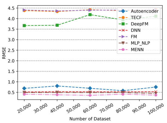
Figure 9.
The RMSE of models changes with dataset size.
As can be seen from Figure 7 to Figure 9, the changes in MENN, DNN and MLP_NLP are small as the dataset size increasing, and the advantage of these models are smaller prediction errors and better performance. The evaluation metrics of Autoencoder fluctuate slightly with dataset size. As the dataset increases, the Autoencoder’s prediction error increases. When the dataset continues to increase, the Autoencoder’s prediction error begins to decrease. Similarly, the evaluation metric values of the TECF model and the FM model with the least satisfactory performance also appear to vary as increasing dataset size. The fluctuation range of the prediction error of the DeepFM model is larger than that of other models. It is plausible that the fluctuation of DeepFM model is not only affected by the DNN model, but also by the FM model. Given the dual impact of the fluctuations of the FM and the DNN, the fluctuation range of the DeepFM is slightly higher than other models. In addition, looking at the trend in Figure 7, Figure 8 and Figure 9, the error values of the Autoencoder, MLP_NLP, DNN, and MENN models that are based on DNN are relatively close. The evaluation metric values of these models are much smaller than TECF, FM, and DeepFM. This phenomenon occurs because TECF and FM are not based on a DNN model, and DeepFM uses a DNN architecture, offering better performance.
Figure 10 and Figure 11 are visualizations of embedding text comment data on the two datasets “Electronic” and “Book”, respectively. These three-dimensional visualizations were generated using the t-SNE dimensionality reduction method. After summarizing these text comment data into concise abstract text, the abstract text is converted into feature vectors that can be embedded in the model. In practice, these feature vectors are multi-dimensional vectors. To facilitate visual display, these text embedding vectors are reduced to 3-D vectors. Each dot in the figure represents a 3-D vector, and this 3-D vector represents a user’s comment record on the corresponding product, portraying it an example of user comment text vector embedding. As shown in Figure 10 and Figure 11, the visual images of many users’ comments text are clustered together and very similar, which means that the comment text they represent has similar meanings. In general, the user preferences reflected by the user’s textual comments are consistent with the trend of the user’s rating on the items. Users with a rating of 5 have a different comment tendency compared to those with a rating of 1. This suggests that spatial distance influences the user-generated text embedding vectors with different comment tendencies. Users with similar preferences may have a similar comment tendency on the product, resulting in the text embedding vectors generated being relatively similar in spatial distance and thus clustered. When a user’s rating for an item is less than 3, the user’s preference on the item is low. In Figure 10 and Figure 11, blue dots are used to indicate the embedding of these users’ text comments. In the legend, “class 1” is used to represent such data. Conversely, when the user’s rating for an item is greater than 3, the user prefers the corresponding item. The red dots indicate the embedding of these users’ text comments. In the legend, “class 2” is used to represent such data. Clearly, most text embedding vectors with similar degrees of preference are clustered, indicating that the tendency of related text comments is relatively close. The embedding vector formed by text comments can help DNN models better mine user preferences.
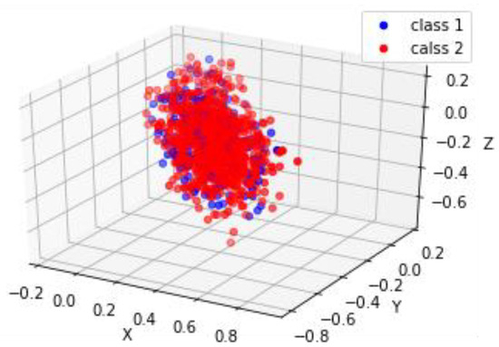
Figure 10.
Electronic vector.
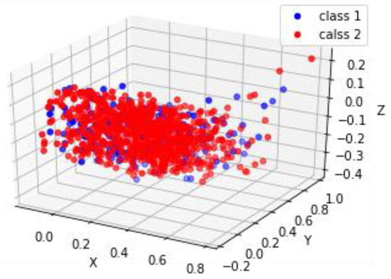
Figure 11.
Book vector.
5. Discussion
Through performance comparisons with other baseline models, it was found that the proposed MENN model achieved better performance on both the “Electronic” and “Book” datasets, validating the effectiveness of the text and numerical information embedding deep neural network architecture. Traditional models like FM and TECF perform poorly in handling complex user preference patterns due to their lack of deep feature representation capabilities. Although DeepFM incorporates deep learning components, the limitations of its FM part still restrict overall performance improvement. In contrast, models based purely on DNN architectures (such as Stacked Autoencoders, DNN, and MLP_NLP) demonstrate stronger feature learning capabilities. However, the MENN model further exploits the synergistic effects of multimodal data through an effective parallel embedding strategy of numerical and textual information, achieving significant performance improvements across all evaluation metrics. This result not only demonstrates the superiority of deep neural networks in user preference mining tasks but also highlights the critical role of multimodal information fusion strategies in enhancing prediction accuracy, providing new technical insights and empirical support for the field of user preference modeling.
6. Conclusions
This study proposes a multi-form information embedding deep neural network that integrates numerical and textual data through parallel embedding architectures for enhanced user preference mining. The approach addresses single-modality limitations by leveraging complementary behavioral and semantic information.
Experimental results demonstrate that the proposed MENN model significantly outperforms baseline methods across multiple datasets. The key finding reveals that numerical embeddings effectively capture behavioral patterns while textual embeddings provide semantic context, with their synergistic fusion enabling comprehensive multi-dimensional user preference modeling and superior predictive accuracy.
However, this study also has some limitations. The main issue lies in the performance during cold-start scenarios. Although multimodal fusion helps alleviate data sparsity, the prediction accuracy for new users and new items still needs improvement. Future research can explore more effective solutions to the cold-start problem by leveraging “meta-learning.”
Funding
This work was supported by the National Natural Science Foundation of China (No. 72301143; No. 72502110), China Postdoctoral Science Foundation General Project (No. 2025M770770).
Data Availability Statement
The data presented in this study are openly available at https://github.com/helloworld1621/user (accessed on 6 October 2025).
Conflicts of Interest
The author declares no conflict of interest.
References
- Gao, M.; Li, J.Y.; Chen, C.H.; Li, Y.; Zhang, J.; Zhan, Z.H. Enhanced multi-task learning and knowledge graph-based rec-ommender system. IEEE Trans. Knowl. Data Eng. 2023, 35, 10281–10294. [Google Scholar] [CrossRef]
- Cui, Y.; Yu, H.; Guo, X.; Cao, H.; Wang, L. RAKCR: Reviews sentiment-aware based knowledge graph convolutional networks for Personalized Recommendation. Expert Syst. Appl. 2024, 248, 123403. [Google Scholar] [CrossRef]
- Cheng, S.H.; Chen, W.Y.; Liu, W.L.; Zhou, L.; Zhao, H.L.; Kong, W.S.; Qu, H.; Fu, M.S. Dynamic training for handling textual label noise. Appl. Intell. 2024, 54, 11161–11176. [Google Scholar] [CrossRef]
- Alharbe, N.; Rakrouki, M.A.; Aljohani, A. A collaborative filtering recommendation algorithm based on embedding repre-sentation. Expert Syst. Appl. 2023, 215, 119380. [Google Scholar] [CrossRef]
- Kuo, R.J.; Li, S.S. Applying particle swarm optimization algorithm-based collaborative filtering recommender system consid-ering rating and review. Appl. Soft Comput. 2023, 135, 110038. [Google Scholar] [CrossRef]
- Zhu, B.; Guo, D.; Ren, L. Consumer preference analysis based on text comments and ratings: A multi-attribute decision-making perspective. Inf. Manag. 2022, 59, 103626. [Google Scholar] [CrossRef]
- Fonseca, J.; Bacao, F. Tabular and latent space synthetic data generation: A literature review. J. Big Data 2023, 10, 115. [Google Scholar] [CrossRef]
- Gabryel, M.; Kocić, E.; Kocić, M.; Patora-Wysocka, Z.; Xiao, M.; Pawlak, M. Accelerating user profiling in e-commerce using conditional GAN networks for synthetic data generation. J. Artif. Intell. Soft Comput. Res. 2024, 14, 309–319. [Google Scholar] [CrossRef]
- Xiao, Y.; Li, C.; Thürer, M.; Liu, Y.; Qu, T. User preference mining based on fine-grained sentiment analysis. J. Retail. Consum. Serv. 2022, 68, 103013. [Google Scholar] [CrossRef]
- Park, J.; Ahn, H.; Kim, D.; Park, E. GNN-IR: Examining graph neural networks for influencer recommendations in social media marketing. J. Retail. Consum. Serv. 2024, 78, 103075. [Google Scholar] [CrossRef]
- Wang, J.F.; Guo, Y.F.; Yang, L.; Wang, Y.H. Enabling Homogeneous GNNs to Handle Heterogeneous Graphs via Relation Embedding. IEEE Trans. Big Data 2023, 9, 1697–1710. [Google Scholar] [CrossRef]
- Bian, Y.; Ye, R.; Zhang, J.; Yan, X. Customer preference identification from hotel online reviews: A neural network based fi-ne-grained sentiment analysis. Comput. Ind. Eng. 2022, 172, 108648. [Google Scholar] [CrossRef]
- Hanifi, M.; Chibane, H.; Houssin, R.; Cavallucci, D. Problem formulation in inventive design using Doc2vec and Cosine Sim-ilarity as Artificial Intelligence methods and Scientific Papers. Eng. Appl. Artif. Intell. 2022, 109, 104661. [Google Scholar] [CrossRef]
- Qu, S.L.; Guo, G.B.; Liu, Y.; Yao, Y.; Wei, W. Fast discrete factorization machine for personalized item recommendation. Knowl.-Based Syst. 2020, 193, 105470. [Google Scholar] [CrossRef]
- Wang, R.Q.; Jiang, Y.L.; Lou, J.G. TDR: Two-stage deep recommendation model based on mSDA and DNN. Expert Syst. Appl. 2020, 145, 113116. [Google Scholar] [CrossRef]
- Liu, W.; Zhang, Z.; Bai, Y.; Liu, Y.; Yang, A.; Li, J. A DeepFM-based non-parametric model enabled big data platform for predicting passenger car sales in sustainable way. IEEE Trans. Intell. Transp. Syst. 2023, 24, 16018–16028. [Google Scholar] [CrossRef]
- Li, D.; Wang, C.; Li, L.; Zheng, Z. Collaborative filtering algorithm with social information and dynamic time windows. Appl. Intell. 2022, 52, 5261–5272. [Google Scholar] [CrossRef]
- Wu, P.; Miao, Z.D.; Wang, K.; Gao, J.F.; Zhang, X.J.; Lou, S.W.; Yang, C.J. FA-SconvAE-LSTM: Feature-Aligned Stacked Convolutional Autoencoder with Long Short-Term Memory Network for Soft Sensor Modeling. Eng. Appl. Artif. Intell. 2025, 150, 110535. [Google Scholar] [CrossRef]
- Çolhak, F.; Ecevit, M.İ.; Dağ, H.; Creutzburg, R. SecureReg: Combining NLP and MLP for Enhanced Detection of Malicious Domain Name Registrations. In Proceedings of the 2024 International Conference on Electrical, Computer and Energy Tech-nologies, Sydney, Australia, 25–27 July 2024; pp. 1–6. [Google Scholar] [CrossRef]
Disclaimer/Publisher’s Note: The statements, opinions and data contained in all publications are solely those of the individual author(s) and contributor(s) and not of MDPI and/or the editor(s). MDPI and/or the editor(s) disclaim responsibility for any injury to people or property resulting from any ideas, methods, instructions or products referred to in the content. |
© 2025 by the author. Licensee MDPI, Basel, Switzerland. This article is an open access article distributed under the terms and conditions of the Creative Commons Attribution (CC BY) license (https://creativecommons.org/licenses/by/4.0/).