Assessing the Role of Vaccination in the Control of Hand, Foot, and Mouth Disease Transmission

Abstract

The impact of vaccination on the dynamics of hand, foot, and mouth disease (HFMD) transmission is explored in this paper, considering a fractional-order derivative system of equations. This model provides vaccination strategies and characterizes local and global stability using Lyapunov functions. This work computes the basic reproduction number ($R_0$) to represent the endemic and epidemic scenarios. Additionally, sensitivity analysis was performed to identify the most critical parameters responsible for the disease dissemination. Our results indicate that vaccination plays a crucial role in controlling HFMD, significantly reducing its prevalence. These findings align with existing research, supporting the importance of effective vaccination strategies and public health interventions against HFMD. The fractional-order model captures the memory effect in infectious disease dynamics, providing further insight into modeling HFMD transmission compared to a traditional integer-order model. The results would contribute to effective vaccination strategies and public health interventions against HFMD.

1. Introduction

This paper involves incorporating vaccination into the study of hand, foot, and mouth disease (HFMD) transmission dynamics to understand the effects of different immunization strategies on outbreaks within populations. Vaccination has the potential to significantly lower the basic reproduction number ($R_0$), the number of secondary infections produced by the average infected person. The immunization of a large part of the population susceptible to infection breaks the chain of transmission, which will reduce the spread of the virus. In communities where vaccination is highly prevalent, HFMD outbreaks may remain impressively low due to fewer people being susceptible to the virus [1,2,3,4]. In addition, vaccination may assist in herd immunity, whereby unvaccinated populations tend to benefit from the reduced virus circulation. In addition, vaccine efficacy and coverage rates, and even age distribution among the vaccinated population [5], might be other factors influencing the effectiveness of vaccination in HFMD control. This can be accomplished using mathematical modeling and epidemiological studies to determine what different vaccination scenarios would yield an effect, thereby assisting program designers in developing specific immunization programs that would limit the burden of HFMD in at-risk populations.

Therefore, it is important to use fractional-order models to analyze transmission dynamics and intervention strategies associated with HFMD to fill the existing literature gap. Fractional-order differential equations are a sophisticated mathematical framework incorporating memory effects and hereditary characteristics inherent in biological processes, including infectious disease dissemination. On the contrary, fractional-order models can capture all these complexities in disease propagation and control strategies by using fractional derivatives, which are believed to represent the time-dependent manner in which a system’s state depends on the previous context. In the context of HFMD, fractional-order models can be used to investigate the long-term impact of vaccination strategies where variations in individual immunity levels, vaccine efficacy, and waning immunity are considered. These models come in handy for capturing scenarios where the population does exhibit heterogeneity about vaccination programs, such as differences in adherence to the recommended immunization schedules or changes in social contact behavior. Combining fractional dynamics with standard compartmental structures like SIR or SEIR will offer a better way for researchers to capture how vaccination impacts the effective reproduction number of disease ($R_0$) under different times and demographic settings [6,7,8,9].

The modes of transmission of infectious diseases represent a variety of mechanisms, generally classified into two broad categories: direct and indirect. Direct transmission may occur through actual physical contact, respiratory droplets, or several body fluids, resulting in the transfer of infectious agents from one host to another. Indirect transmission involves intermediate agents such as fomites (inanimate infected objects), vectors like mosquitoes, and air particles [10,11]. Mathematical modeling further elucidates the complex nature of disease spread and provides critical tools for describing and predicting transmission dynamics. The basic notions include the basic reproduction number, $R_0$, defined as the average number of secondary infections produced by one infected individual in a wholly susceptible population, indicating a pathogen’s contagiousness. SIR and SEIR compartment models have been some of the most used compartment models to simulate the dynamics of diseases within populations by partitioning individuals into different compartments depending on their disease status [12,13,14,15,16,17].

Agent-based models explicitly simulate the individual-to-individual interactions within a population and hence provide further details; they are thus much better suited to capturing heterogeneous mixing patterns and individual behavior. Stochastic models incorporate randomness in the transmission process; this is appropriate for modeling the natural variability and, in particular, the unpredictability of real-world disease transmission. Network model approaches that explicitly represent populations as interconnected networks of individuals offer insight into how the structure of social interactions drives disease dynamics. Besides these mathematical methods, a significant contribution is seen in modern epidemiology in data-driven approaches. Using data around surveillance analysis and genomic epidemiology, model-based approaches use real-time data and large datasets to track disease spread, identify risk factors, and optimize intervention strategies.

Another key aspect involves intervention modeling, such as different vaccination scenarios, simulations for quarantine and isolation policies, and social distancing measures. These models enable the modeling of the potential impacts of various interventions on disease containment and control. In reality, such models are used in planning pandemic responses, and governments and health agencies use them to forecast outbreaks, assess the effectiveness of interventions, and inform resource allocation. But once again, such models are hostage to the quality of data, the accuracy of the assumptions behind them, and their ability to capture uncertainty and behavior changes in the population. Nonetheless, model techniques will remain invaluable for scientific insight into and the management of infectious disease spread.

2. Preliminaries

This section presents basic definitions, theorems, and results connected with the stability, existence, and uniqueness of our model, which is developed based on the Caputo fractional derivative. Such a mathematical toolkit provides a complete setting for scrutinizing the model’s dynamic behavior. Moreover, we start by recalling some relevant definitions of the Caputo fractional derivatives, fixed-point theorems, and stability criteria. These are critical elements to help validate the robustness and reliability of our model for capturing the dynamics of HFMD.

Definition 1 

([18]). The integral formula for the Caputo fractional derivative of order $(\alpha \in (m-1,m\left]\right)$ for a function $\left(h\right(x\left)\right)$ that is $\left(mth\right)$-differentiable is given by the following:

$${}_0{D}_t^{\alpha }h\left(x\right)={\displaystyle \frac{1}{\mathrm{\Gamma }(m-\alpha )}}{\int }_0^x{(x-t)}^{m-\alpha -1}{h}^{\left(m\right)}\left(t\right),dt,m=\lceil \alpha \rceil .$$

Theorem 1 

([19]). Let $T:Y\to Y$ be a contractive operator on a complete metric space $(Y,\mathit{dist})$. Then, T has a unique fixed point $z^{\ast }\in Y$ such that $T\left(z^{\ast }\right)=z^{\ast }$. Additionally, T satisfies the following contraction condition:

$$\mathit{dist}\left(T\right(z),T(w\left)\right)\le K\mathit{dist}(z,w),\mathit{for}\mathit{all}z,w\in Y,$$

where $0<K<1$. This result guarantees the existence and uniqueness of the fixed point and provides a method to approximate it iteratively due to the contractive nature of T.

Definition 2 

([20]). For a function $f:\mathbb{R}\to \mathbb{R}$ that is integrable and a fractional order $0<\alpha \le 1$, the fractional integral of f of order α is defined as

$${\mathcal{I}}^{\alpha }f\left(y\right)={\displaystyle \frac{1}{\mathrm{\Gamma }\left(\alpha \right)}}{\int }_0^y{(y-t)}^{\alpha -1}f\left(t\right)dt.$$

Lemma 1 

([21]). The Laplace transform of the Caputo fractional derivative is expressed as follows:

$$\mathcal{L}{\{}_0{D}_t^{\alpha }g\left(t\right)\}=s^{\alpha }\mathcal{L}\left\{g\left(t\right)\right\}-s^{\alpha -1}g\left(0\right),0<\alpha <1.$$

This expression indeed contains the relationship between the fractional derivative and its Laplace transform, along with the initial condition $g\left(0\right)$, as per the definition by Caputo.

Theorem 2 

([22]). The equilibrium solutions $z^{\ast }$ of the Caputo fractional differential equation system

$${}_0{D}_t^{\alpha }z\left(t\right)=g(t,x),z\left(t_0\right)=z_0$$

are locally asymptotically stable (LAS) if the eigenvalues ${\lambda }_j$ of the Jacobian matrix ${\displaystyle \frac{\partial g}{\partial z_j}}$, evaluated at these equilibrium points, satisfy the following condition:

$$\left|arg\left({\lambda }_j\right)\right|=\pi >{\displaystyle \frac{\alpha \pi }{2}},0<\alpha <1,\forall j=1,\dots ,n.$$

This condition guarantees the stability by demanding that the arguments of the eigenvalues be within a defined range about the fractional order α.

Theorem 3 

([23]). Let $z\left(t\right)\in {\mathbb{R}}^{+}$ be a continuous and differentiable function. For a given $z^{\ast }\in {\mathbb{R}}^{+}$ and $0<\alpha <1$, the following inequality holds for any time instant $t\ge t_0$:

$${}_0{D}_t^{\alpha }\left[z\left(t\right)-z^{\ast }-z^{\ast }ln{\displaystyle \frac{z\left(t\right)}{z^{\ast }}}\right]\le \left(1-{\displaystyle \frac{z\left(t\right)}{z^{\ast }}}\right){}_0{D}_t^{\alpha }z\left(t\right).$$

This result follows from the properties of the Caputo fractional derivative and highlights the relationship between the function $z\left(t\right)$ and its equilibrium value $z^{\ast }$.

Theorem 4 

([24]). Let $z^{\ast }$ be an equilibrium point of the fractional-order differential equation ${}_0{D}_t^{\alpha }z\left(t\right)=g(t,z)$, where $\mathrm{\Omega }\subset {\mathbb{R}}^m$ is a domain containing $z^{\ast }$. Define a Lyapunov candidate function $U(t,z):[0,+\infty )\times \mathrm{\Omega }\to \mathbb{R}$ that satisfies the following conditions:

I. 

There exist continuous, positive definite functions $W_1\left(z\right)$ and $W_2\left(z\right)$ on Ω such that

$$W_1\left(z\right)\le U(t,z)\le W_2\left(z\right),\forall z\in \mathrm{\Omega },\forall t\ge 0.$$

II. 

The fractional derivative of U satisfies

$${}_0{D}_t^{\alpha }U(t,z)\le -W_3\left(z\right),\forall z\in \mathrm{\Omega },\forall t\ge 0,\alpha \in (0,1),$$

where $W_3\left(z\right)$ is a continuous, positive definite function on Ω . Under these conditions, the equilibrium point $z^{\ast }$ is globally asymptotically stable.

This theorem extends the Lyapunov stability approach to fractional-order systems. The conditions imposed on $U(t,z)$ ensure it acts as a Lyapunov function, providing bounds on the system’s behavior and guaranteeing that $z\left(t\right)\to z^{\ast }$ as $t\to \infty$. The fractional derivative condition emphasizes that U decreases along trajectories, leading to stability.

The Caputo formulation of the fractional derivative is preferred in epidemiological modeling because it is compatible with the conventional initial conditions usually expressed as integer-order derivatives [25]. This compatibility makes it easier to incorporate real data into the models. In addition, the Caputo derivative provides a more natural physical interpretation, especially for biological systems, because of memory effects where past states affect current and future dynamics [26]. This feature is of major importance in epidemiology since the historical development of disease transmission significantly impacts current-day transmission values. The Caputo derivative has been more flexible in representing complex systems, enabling the accurate characterizations of non-local dynamics and memory effects that are not captured by traditional integer-order models. In addition, it provides an easy transition from the fractional-order to the integer-order model, which really simplifies the comparison and transition across different modeling approaches [27].

Our article is organized as follows: We begin with the proposed model, introducing the fractional model and the relevant proofs of existence and uniqueness. This is followed by a section dedicated to equilibrium stability analysis. Next, we include a section on endemic equilibrium. Finally, we conclude with a discussion and numerical results section.

3. Proposed Model for HFMD Dynamical Spreading

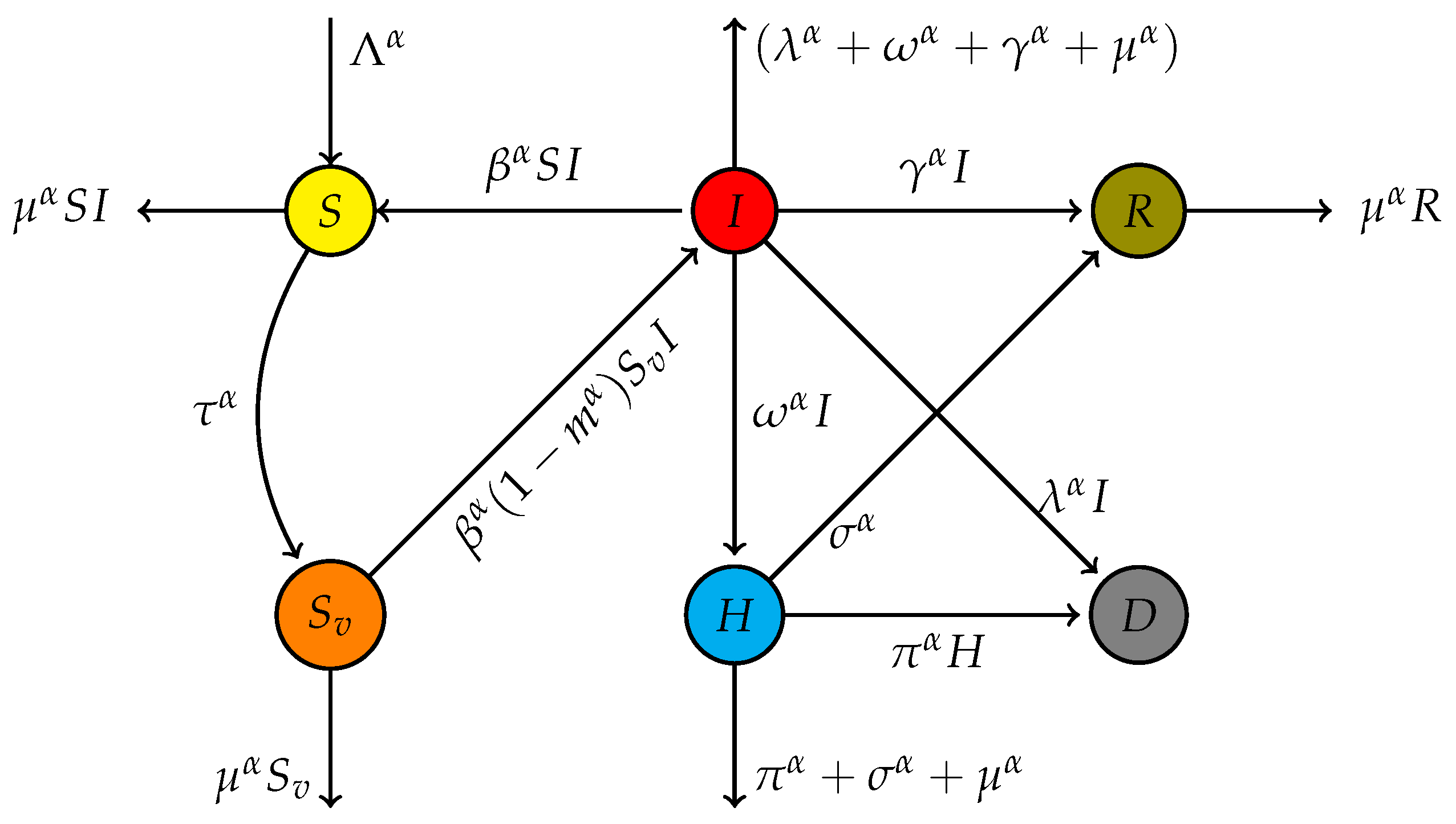
In this section, we introduce a system of differential equations incorporating fractional derivatives to model the dynamical spreading of hand, foot, and mouth disease (HFMD). Using fractional derivatives allows for a more accurate representation of memory and hereditary properties in the disease transmission process. This approach captures the complex dynamics of HFMD more effectively than traditional integer-order models. The equations presented here reflect these advanced modeling techniques, providing a robust framework for analyzing the spread of HFMD under various realistic scenarios, including vaccination efficiency. Figure 1 illustrates the interconnections between compartments, with all parameters clearly defined, while the system of Equation (1) mathematically describes the dynamic behavior depicted in Figure 1.

$$\begin{array}{cc}\hfill & {}_0{D}_t^{\alpha }S={\mathrm{\Lambda }}^{\alpha }-{\beta }^{\alpha }SI-\left({\tau }^{\alpha }+{\mu }^{\alpha }\right)S,\hfill \\ \hfill & {}_0{D}_t^{\alpha }{S}_v=-{\beta }^{\alpha }\left(1-m^{\alpha }\right)S_{v}I+{\tau }^{\alpha }S-{\mu }^{\alpha }{S}_v,\hfill \\ \hfill & {}_0{D}_t^{\alpha }I={\beta }^{\alpha }SI+{\beta }^{\alpha }\left(1-m^{\alpha }\right)S_{v}I-\left({\delta }^{\alpha }+{\omega }^{\alpha }+{\gamma }^{\alpha }+{\mu }^{\alpha }\right)I,\hfill \\ \hfill & {}_0{D}_t^{\alpha }H={\omega }^{\alpha }I-\left({\pi }^{\alpha }+{\sigma }^{\alpha }+{\mu }^{\alpha }\right)H,\hfill \\ \hfill & {}_0{D}_t^{\alpha }R={\gamma }^{\alpha }I+{\sigma }^{\alpha }H-{\mu }^{\alpha }R,\hfill \\ \hfill & {}_0{D}_t^{\alpha }D={\delta }^{\alpha }I+{\pi }^{\alpha }H.\hfill \end{array}$$

(1)

With the following initial conditions:

$$S\left(0\right)\ge 0,S_v\left(0\right)\ge 0,I\left(0\right)\ge 0,H\left(0\right)\ge 0,R\left(0\right)\ge 0,D\left(0\right)\ge 0.$$

Table 1. Descriptions of the variables and parameters in the proposed model (1).

Variable	Description
S	The number of the susceptible population.
$S_v$	The number of the susceptible vaccinated population.
I	The number of the infectious population.
H	The number of the hospitalized population.
R	The number of the recovered population.
D	The number of the dead population.
Parameter	Description	Sample Value Utilized
${\mathrm{\Lambda }}^{\alpha }$	Recruitment rate	Assumed to range between 300 and 500
${\mu }^{\alpha }$	Natural death rate	Assumed to range between 1 and 5 per day
${\beta }^{\alpha }$	Transmission rate	0.3 to 0.5 per day, [28]
${\tau }^{\alpha }$	Vaccination rate	Varies, [5]
${\gamma }^{\alpha }$	Recovery from infection rate	0.1 to 0.14 per day, [29]
${\sigma }^{\alpha }$	Recovery from infection while in hospital	0.2 to 0.3 per day, [30]
${\omega }^{\alpha }$	Hospital admission rate	0.01 to 0.05 per day, [30]
${\delta }^{\alpha }$	Death rate of infected population	0.0001 per day, [31]
${\pi }^{\alpha }$	Death rate of hospitalized population	Taken from References [29,30]: 0.0002 per day
$m^{\alpha }$	Efficacy of vaccine for preventing infection	Taken from Reference [32]: $90\%$

summarizes the detailed descriptions of the variables and parameters used in the proposed model. The model tracks different groups of the population based on their health state. S is the class of the susceptible population, and $S_v$ accounts for the vaccinated susceptible individuals. I denotes the number of infected, H—those hospitalized, and R—those recovered. The parameters describe basic model dynamics: ${\mathrm{\Lambda }}^{\alpha }$ describes new inflows into the population, ${\mu }^{\alpha }$ describes the mortality rate, and ${\beta }^{\alpha }$ describes the rate at which an infection spreads in the population. The vaccination efforts are described through ${\tau }^{\alpha }$, while through ${\gamma }^{\alpha }$ and ${\sigma }^{\alpha }$, the recovery rate models describe the infected and hospitalized populations. Hospitalization and death rates are described through ${\omega }^{\alpha }$, ${\delta }^{\alpha }$, and ${\pi }^{\alpha }$. Finally, $m^{\alpha }$ describes the efficiency of the vaccine in impeding the infection. The above variables and parameters define the dynamics of infection, recovery, hospitalization, and population mortality.

3.1. Positivity and Boundedness

In a mathematical model for epidemiology, positivity and boundedness are the two major features that guarantee the model operates in a way that shows real population dynamics. Positivity guarantees that no model variable, representing the number of susceptible, infected, or recovered individuals at any given time, assumes a negative value, which does not make biological sense. Boundedness means that the model variables do not grow boundlessly but rather stay within the confines of the total size of a finite population. These characteristics are crucial for ensuring the model’s validity and reliability in accurately portraying the dissemination and management of diseases.

Define the region $\mathrm{\Omega }=\left\{(S\left(t\right),S_v\left(t\right),I\left(t\right),H\left(t\right),R\left(t\right),D\left(t\right)\in {\mathbb{R}}_{+}^6:S+S_v+I+H+R\right.$$\left.+D\le {\displaystyle \frac{{\mathrm{\Lambda }}^{\alpha }}{{\mu }^{\alpha }}}\right\}$. The following theorem shows that $\mathrm{\Omega }$ is positively invariant.

The superscript $\alpha$ in Equation (1) functions simultaneously as the fractional order and the power, playing a critical role in capturing the memory effect and non-local behavior of the model. This dual functionality allows the model to account for the influence of past states on current and future dynamics, which is particularly significant in epidemiological modeling. By incorporating historical disease spread, the model enhances the ability to predict and control future transmission.

Theorem 5 

The non-negative region Ω that includes the solutions of Model (1) ’s equations is positively invariant for $t\ge 0$.

Proof. 

Let the total population $T\left(t\right)$ be the sum of the model’s components, i.e., $T\left(t\right)=S\left(t\right)+S_v\left(t\right)+I\left(t\right)+H\left(T\right)+R\left(t\right)+D\left(t\right)$. Then,

$$\begin{array}{cc}\hfill {}_0{D}_t^{\alpha }T& ={}_0{D}_t^{\alpha }S+{}_0{D}_t^{\alpha }{S}_v+{}_0{D}_t^{\alpha }I+{}_0{D}_t^{\alpha }H+{}_0{D}_t^{\alpha }R+{}_0{D}_t^{\alpha }D\hfill \\ \hfill & ={\mathrm{\Lambda }}^{\alpha }-{\mu }^{\alpha }S-{\mu }^{\alpha }{S}_v-{\mu }^{\alpha }I-{\mu }^{\alpha }H-{\mu }^{\alpha }R\hfill \\ \hfill & ={\mathrm{\Lambda }}^{\alpha }-{\mu }^{\alpha }T\hfill \end{array}$$

Therefore, we conclude that

$${}_0{D}_t^{\alpha }T+{\mu }^{\alpha }T={\mathrm{\Lambda }}^{\alpha }.$$

(2)

To proceed with the proof, let $\mathcal{L}\left\{T\left(t\right)\right\}=\widehat{T}\left(s\right)$ be the Laplace transform of $T\left(t\right)$ with the initial condition $T\left(0\right)=T_0$. By the application of the Laplace transform on Equation (2), we have

$$\begin{array}{cc}\hfill \mathcal{L}{\{}_0{D}_t^{\alpha }T+{\mu }^{\alpha }T\}& =\mathcal{L}\left\{{\mathrm{\Lambda }}^{\alpha }\right\}\hfill \\ \hfill s^{\alpha }\widehat{T}\left(s\right)-s^{\alpha -1}{T}_0+{\mu }^{\alpha }\widehat{T}\left(s\right)& ={\displaystyle \frac{{\mathrm{\Lambda }}^{\alpha }}{s}}\hfill \\ \hfill & \widehat{T}\left(s\right)={\displaystyle \frac{{\mathrm{\Lambda }}^{\alpha }+s^{\alpha }{T}_0}{s(s^{\alpha }+{\mu }^{\alpha })}}\hfill \\ \hfill & ={\displaystyle \frac{{\mathrm{\Lambda }}^{\alpha }}{s^{\alpha +1}\left(1+\frac{{\mu }^{\alpha }}{s^{\alpha }}\right)}}+{\displaystyle \frac{T_0}{s\left(1+\frac{{\mu }^{\alpha }}{s^{\alpha }}\right)}}\hfill \\ \hfill \widehat{T}\left(s\right)& ={\displaystyle \frac{{\mathrm{\Lambda }}^{\alpha }}{{\mu }^{\alpha }}}\sum _{n=0}^{\infty }{\displaystyle \frac{{(-{\mu }^{\alpha })}^{n+1}}{s^{(n+1)\alpha +1}}}+T_0\sum _{n=0}^{\infty }{\displaystyle \frac{{(-{\mu }^{\alpha })}^n}{s^{n\alpha +1}}}.\hfill \end{array}$$

(3)

To find $T\left(t\right)$, we take Laplace inverse to both sides of Equation (3) to obtain the following:

$$\begin{array}{cc}\hfill {\mathcal{L}}^{-1}\left\{\widehat{T}\left(s\right)\right\}& ={\mathcal{L}}^{-1}\left\{{\displaystyle \frac{{\mathrm{\Lambda }}^{\alpha }}{{\mu }^{\alpha }}}\sum _{n=0}^{\infty }{\displaystyle \frac{{(-{\mu }^{\alpha })}^{n+1}}{s^{(n+1)\alpha +1}}}+T_0\sum _{n=0}^{\infty }{\displaystyle \frac{{(-{\mu }^{\alpha })}^n}{s^{n\alpha +1}}}\right\}\hfill \\ \hfill & ={\displaystyle \frac{{\mathrm{\Lambda }}^{\alpha }}{{\mu }^{\alpha }}}\sum _{n=0}^{\infty }{\displaystyle \frac{{(-{\mu }^{\alpha }{t}^{\alpha })}^{n+1}}{\mathrm{\Gamma }(n\alpha +\alpha +1)}}+T_0\sum _{n=0}^{\infty }{\displaystyle \frac{{(-{\mu }^{\alpha }{t}^{\alpha })}^n}{\mathrm{\Gamma }(n\alpha +1)}}\hfill \\ \hfill T\left(t\right)& ={\displaystyle \frac{{\mathrm{\Lambda }}^{\alpha }}{{\mu }^{\alpha }}}{E}_{\alpha ,1}(-{\mu }^{\alpha }{t}^{\alpha })+T_0{E}_{\alpha ,\alpha +1}(-{\mu }^{\alpha }{t}^{\alpha }).\hfill \end{array}$$

(4)

According to the Mittag–Leffler function property

$$E_{c,d}\left(x\right)=x{E}_{c,c+d}\left(x\right)+{\displaystyle \frac{1}{\mathrm{\Gamma }\left(d\right)}},$$

Equation (4) becomes

$$T\left(t\right)=(T_0-{\mathrm{\Lambda }}^{\alpha })E_{\alpha ,\alpha +1}(-{\mu }^{\alpha }{t}^{\alpha })+{\displaystyle \frac{{\mathrm{\Lambda }}^{\alpha }}{{\mu }^{\alpha }}}.$$

Thus, $lim\; supT\left(t\right)\le {\displaystyle \frac{{\mathrm{\Lambda }}^{\alpha }}{{\mu }^{\alpha }}}$. This completes the proof. □

3.2. Existence and Uniqueness

We can prove the existence and uniqueness of the solution for the fractional epidemic model of HFMD by applying mathematical methodologies, mainly fixed-point theorems. The accent is on the Banach fixed-point theorem. This model, which combines fractional derivatives, better describes the dynamics of the disease due to the presence of memory in the population. The existence of a solution guarantees a well-defined trajectory of the disease spread for any given set of initial conditions. On the other hand, uniqueness guarantees that the behavior is deterministic; the course of the disease progression can thus be predicted and is not dependent on arbitrary choices. These properties are usually demonstrated by converting the system to an appropriate integral form and showing that the associated operator satisfies the fixed-point theorem conditions to guarantee the solution’s existence and uniqueness. The conclusion here is that the model produces a reliable prediction concerning the dynamics of the epidemic over time.

Theorem 6 

The equations of System (1) satisfy the Lipschitz continuous conditions for $K_j\ge 0,j=1,2,3,4,5.$

Proof. 

Rewrite the equations of System (1) in a steady-state mode as follows:

$$\begin{array}{cc}& g_1\left(S\right)={\mathrm{\Lambda }}^{\alpha }-({\tau }^{\alpha }+{\mu }^{\alpha })S-{\beta }^{\alpha }SI,\hfill \\ & g_2\left(S_v\right)={\tau }^{\alpha }S-{\mu }^{\alpha }{S}_v-\beta (1-m^{\alpha })S_{v}I,\hfill \\ & g_3\left(I\right)={\beta }^{\alpha }SI+{\beta }^{\alpha }(1-m^{\alpha })S_{v}I-({\delta }^{\alpha }+{\omega }^{\alpha }+{\mu }^{\alpha }+{\gamma }^{\alpha })I,\hfill \\ & g_4\left(H\right)={\omega }^{\alpha }I-({\pi }^{\alpha }+{\sigma }^{\alpha }+{\mu }^{\alpha }),\hfill \\ & g_5\left(R\right)={\gamma }^{\alpha }I+{\sigma }^{\alpha }H-{\mu }^{\alpha }R,\hfill \end{array}$$

Upon applying Theorem 1, we obtain the following:

$$\begin{array}{cc}\hfill ∥g_1\left(S\right)-g_1\left(S^{\prime }\right)∥& =∥({\tau }^{\alpha }+{\mu }^{\alpha })\left(S-S^{\prime }\right)+{\beta }^{\alpha }I\left(S-S^{\prime }\right)∥\hfill \\ & \le |{\tau }^{\alpha }+{\mu }^{\alpha }|∥S-S^{\prime }∥+|{\beta }^{\alpha }|\parallel I\parallel ∥S-S^{\prime }∥\hfill \\ & \le \left(\right|{\tau }^{\alpha }+{\mu }^{\alpha }|+|{\beta }^{\alpha }|{\max }_{t\in [0,T]}\parallel I\parallel )∥S-S^{\prime }∥\hfill \\ & =K_1∥S-S^{\prime }∥\hfill \end{array}$$

where $K_1=|{\tau }^{\alpha }+{\mu }^{\alpha }|+|{\beta }^{\alpha }|{\max }_{t\in [0,T]}\parallel I\parallel <\infty$.

Similarly, the following results can be obtained:

$$\begin{array}{cc}\hfill ∥g_2\left(S_v\right)-g_2\left(S_v^{\prime }\right)∥& \le K_2\parallel S_v-S_v^{\prime }\parallel \hfill \\ \hfill ∥g_3\left(I\right)-g_3\left(I^{\prime }\right)∥& \le K_3\parallel I-I^{\prime }\parallel \hfill \\ \hfill ∥g_4\left(H\right)-g_4\left(H^{\prime }\right)∥& \le K_4\parallel H-H^{\prime }\parallel \hfill \\ \hfill ∥g_5\left(R\right)-g_5\left(R^{\prime }\right)∥& \le K_5\parallel R-R^{\prime }\parallel \hfill \end{array}$$

where $K_2=|{\mu }^{\alpha }|+|{\beta }^{\alpha }(1-m^{\alpha })|{max}_{t\in [0,T]}\parallel I\parallel <\infty$, $K_3=|{\beta }^{\alpha }|{max}_{t\in [0,T]}\parallel S\parallel +|{\beta }^{\alpha }(1-m^{\alpha })|{max}_{t\in [0,T]}∥S_v∥+|{\delta }^{\alpha }+{\omega }^{\alpha }+{\gamma }^{\alpha }+{\mu }^{\alpha }|<\infty$, $K_4=|{\pi }^{\alpha }+{\sigma }^{\alpha }+{\mu }^{\alpha }|<\infty ,\mathrm{and}{K}_5=\left|{\mu }^{\alpha }\right|<\infty$, which completes the proof. □

Lemma 2 

Volterra integral equation form can be used to represent the system of equations in Model (1).

Proof. 

Consider the system of equations in Model (1):

$${}_0{D}_t^{\alpha }{x}_j\left(t\right)=g_j(t,x_j),j=1,\cdots ,5.$$

(5)

By an application of Definition (2) to both sides of Equation (5), we obtain

$${\mathcal{I}}^{\alpha }{(}_0{D}_t^{\alpha }{x}_j\left(t\right))={\mathcal{I}}^{\alpha }\left(g_j(t,x_j)\right),j=1,\cdots ,8.$$

(6)

The left-hand side reduces to $x_j\left(t\right)-x_j\left(0\right)$ and hence, Equation (6) becomes

$$x_j\left(t\right)-x_j\left(0\right)={\displaystyle \frac{1}{\mathrm{\Gamma }\left(\alpha \right)}}{\int }_0^t{(t-u)}^{\alpha -1}{g}_j(u,x_j)du,\mathrm{for}\mathrm{all}j.$$

(7)

Thus, the proof is completed, and the system of equations in Model (1) is converted to the following equivalent system of Volterra integral equations:

$$x_j\left(t\right)=x_j\left(0\right)+{\displaystyle \frac{1}{\mathrm{\Gamma }\left(\alpha \right)}}{\int }_0^t{g}_j(u,x_j){(t-u)}^{\alpha -1}du,\mathrm{for}\mathrm{all}j.$$

(8)

□

Theorem 7 

([33]). For $0<\alpha <1$ and $G=[0,u]\subseteq \mathbb{R},J=[x_j\left(0\right)-k,x_j\left(0\right)+k]$. Let $g_j:G\times J⟶\mathbb{R}$ satisfy the Lipschitz condition and be continuous and bounded, $i.e.,$ ∃ unique $M_j>0,\left|\right|g_j\left(x\right)\left|\right|<M_j$, where $M_j={max}_{t\in [0,u]}\left|\right|g_j\left(x\right)\left|\right|$. If ${\displaystyle \frac{K_j{\ell }_j}{M_j}}<1$, then ∃ only one solution for the initial value problem (1), namely, $x_j\in C[0,u^{\ast }]$, where $u^{\ast }=min\left\{u,{\left({\displaystyle \frac{{\ell }_j\mathrm{\Gamma }(\alpha +1)}{M_j}}\right)}^{{\displaystyle \frac{1}{\alpha }}}\right\}$. $j=1,2,\cdots ,5$.

Proof. 

Let $X=\{x_j\left(t\right)\in C([0,u],{\mathbb{R}}^5):||x_j\left(t\right)-x_j\left(0\right)||\le {\ell }_j$, $j=1,2,\cdots ,5$. Since every sequence $x_j^n$ in X converges to $x_j\in C([0,u],{\mathbb{R}}^5)$ with respect to the infinity norm $\left|\right|·{\left|\right|}_{\infty }$ and x is continuous and $\left|\right|x_j\left(t\right)-x_j\left(0\right)\left|\right|\le {\ell }_j$, then $\forall n\left|\right|x_j^n\left(t\right)-x\left(0\right)\left|\right|\le {\ell }_j$. Thus, X is closed and hence a complete metric space.

Define $\mathcal{F}:X⟶X$ such that

${\displaystyle {\mathcal{F}}_j\left(x\left(t\right)\right)=x_j\left(0\right)+\frac{1}{\mathrm{\Gamma }\left(\alpha \right)}{\int }_0^t{k}_{\alpha }(u,t){\mathcal{F}}_j(u,x_j\left(t\right))du}$, where $k_{\alpha }(u,t)={(t-u)}^{\alpha -1}$. Then,

$$\begin{array}{cc}\hfill \left|\right|{\mathcal{F}}_j\left(x_j\left(t\right)\right)-x_j\left(0\right)\left|\right|& =∥{\displaystyle \frac{1}{\mathrm{\Gamma }\left(\alpha \right)}}{\int }_0^t{k}_{\alpha }(u,t)g_j(u,x_j\left(t\right))du∥,j=1,2,\cdots ,5.\hfill \\ \hfill & \le {\displaystyle \frac{1}{\mathrm{\Gamma }\left(\alpha \right)}}{\int }_0^t{k}_{\alpha }(u,t)\left|\right|g_j(u,x_j\left(t\right))\left|\right|du\hfill \\ \hfill & \le {\displaystyle \frac{M_j}{\mathrm{\Gamma }\left(\alpha \right)}}{\int }_0^t{k}_{\alpha }(u,t)du\hfill \\ \hfill & ={\displaystyle \frac{M_j{t}^{\alpha }}{\mathrm{\Gamma }(\alpha +1)}}\le {\displaystyle \frac{M_j{\left(u^{\ast }\right)}^{\alpha }}{\mathrm{\Gamma }(\alpha +1)}}\le {\ell }_j\hfill \end{array}$$

Therefore, $\left|\right|{\mathcal{F}}_j\left(x_j\left(t\right)\right)-x_j\left(0\right)\left|\right|\le {\ell }_j$, and hence, $\mathcal{F}$ maps X onto itself.

To show that $\mathcal{F}$ is a contraction operator, we assume $y,z\in X$ such that

$$\begin{array}{cc}\hfill \parallel {\mathcal{F}}_j\left(y_j\left(t\right)\right)-{\mathcal{F}}_j\left(z_j\left(t\right)\right)\parallel & =∥{\displaystyle \frac{1}{\mathrm{\Gamma }\left(\alpha \right)}}{\int }_0^t{k}_{\alpha }(u,t)(g_j(u,y_j\left(t\right))-g_j(u,z_j\left(t\right))du∥,j=1,2,\cdots ,5.\hfill \\ \hfill & \le {\displaystyle \frac{1}{\mathrm{\Gamma }\left(\alpha \right)}}{\int }_0^t{k}_{\alpha }(u,t)\left|\right|(g_j(u,y_j\left(t\right))-g_j(u,z_j\left(t\right))\left|\right|du\hfill \\ \hfill & \le {\displaystyle \frac{K_j}{\mathrm{\Gamma }\left(\alpha \right)}}\left|\right|y_j\left(t\right)-z_j\left(t\right)\left|\right|{\int }_0^t{k}_{\alpha }(u,t)du\hfill \\ \hfill & ={\displaystyle \frac{K_j{t}^{\alpha }}{\mathrm{\Gamma }(\alpha +1)}}\left|\right|y_j\left(t\right)-z_j\left(t\right)\left|\right|\hfill \\ \hfill & \le {\displaystyle \frac{K_j{\left(u^{\ast }\right)}^{\alpha }}{\mathrm{\Gamma }(\alpha +1)}}\le {\displaystyle \frac{K_j{\ell }_j}{M_j}}\left|\right|y_j\left(t\right)-z_j\left(t\right)\left|\right|.\hfill \end{array}$$

Therefore, $\parallel {\mathcal{F}}_j\left(y_j\left(t\right)\right)-{\mathcal{F}}_j\left(z_j\left(t\right)\right)\parallel \le {\displaystyle \frac{K_j{\ell }_j}{M_j}}\left|\right|y_j\left(t\right)-z_j\left(t\right)\left|\right|$. Thus, by the assumption ${\displaystyle \frac{K_j{\ell }_j}{M_j}}<1$, $\mathcal{F}$ is a contraction mapping. Therefore, it possesses a unique fixed point. System (1) has a unique solution. □

4. Equilibrium Stability Analysis

4.1. Basic Reproduction Number

The reproduction number, referred to as ${\mathcal{R}}_0$, is an essential threshold parameter that defines the stability of the HFMD epidemic model. This parameter quantifies the mean number of secondary infections that result from one infected individual within a completely susceptible population. If ${\mathcal{R}}_0<1$, then the disease-free equilibrium is stable, and the disease will die out eventually; otherwise, if ${\mathcal{R}}_0>1$, then the disease will spread in the population, and the endemic equilibrium becomes stable. The reproduction number can be obtained by the next-generation matrix method, which involves linearizing the differential equations around the disease-free equilibrium system and then analyzing the transmission and recovery rates. The principal eigenvalue of the resultant matrix yields ${\mathcal{R}}_0$, offering valuable information regarding the likelihood of disease outbreaks and guiding control measures [34]. Following [35], the infection states are divided into transmission and transition matrices as follows:

$$F=\left[\begin{array}{cc}{\beta }^{\alpha }S+{\beta }^{\alpha }(1-m^{\alpha })S_v& 0\\ 0& 0\end{array}\right]\mathrm{and}V=\left[\begin{array}{cc}{\delta }^{\alpha }+{\omega }^{\alpha }+{\gamma }^{\alpha }+{\mu }^{\alpha }& 0\\ -{\omega }^{\alpha }& {\pi }^{\alpha }+{\sigma }^{\alpha }+{\mu }^{\alpha }\end{array}\right].$$

By an application of Theorem (2) in [35], the basic reproduction number is defined as the spectral radius of the matrix $F{V}^{-1}$; i.e., ${\mathcal{R}}_0=\rho \left(F{V}^{-1}\right)$. Therefore, the basic reproduction number can be given by the following expression:

$${\mathcal{R}}_0={\displaystyle \frac{{\mathrm{\Lambda }}^{\alpha }{\beta }^{\alpha }{\mu }^{\alpha }+{\mathrm{\Lambda }}^{\alpha }{\beta }^{\alpha }{\tau }^{\alpha }(1-m^{\alpha })}{{\mu }^{\alpha }({\mu }^{\alpha }+{\tau }^{\alpha })({\delta }^{\alpha }+{\omega }^{\alpha }+{\gamma }^{\alpha }+{\mu }^{\alpha })}}.$$

(9)

4.2. Existence of Equilibria

To find the hand, foot, and mouth free equilibrium point (HFMEEP), we set the right-hand side of Model (1)’s equations to zero to obtain

$$\begin{array}{cc}\hfill {\mathrm{\Lambda }}^{\alpha }-{\beta }^{\alpha }SI-\left({\tau }^{\alpha }+{\mu }^{\alpha }\right)S& =0\hfill \\ \hfill -{\beta }^{\alpha }\left(1-m^{\alpha }\right)S_{v}I+{\tau }^{\alpha }S-{\mu }^{\alpha }{S}_v& =0\hfill \\ \hfill {\beta }^{\alpha }SI+{\beta }^{\alpha }\left(1-m^{\alpha }\right)S_{v}I-\left({\delta }^{\alpha }+{\omega }^{\alpha }+{\gamma }^{\alpha }+{\mu }^{\alpha }\right)I& =0\hfill \\ \hfill {\omega }^{\alpha }I-\left({\pi }^{\alpha }+{\sigma }^{\alpha }+{\mu }^{\alpha }\right)H& =0\hfill \\ \hfill {\gamma }^{\alpha }I+{\sigma }^{\alpha }H-{\mu }^{\alpha }R& =0\hfill \end{array}$$

(10)

The solution of System (10) is given by the following:

$${\mathcal{E}}_0=\left({\displaystyle \frac{{\mathrm{\Lambda }}^{\alpha }}{{\mu }^{\alpha }+{\tau }^{\alpha }}},{\displaystyle \frac{{\tau }^{\alpha }{\mathrm{\Lambda }}^{\alpha }}{{\mu }^{\alpha }\left({\mu }^{\alpha }+{\tau }^{\alpha }\right)}},0,0,0\right).$$

4.3. Local Stability Analysis

This section investigates a local stability analysis of the fractional mathematical model of hand, foot, and mouth disease. The system’s behavior around its equilibrium points, particularly the disease-free equilibrium, is dealt with. Considering the nonlinear system of fractional differential equations, a linear system is considered around the approximate equilibrium solution. Then, the stability of such an equilibrium can be determined by the eigenvalue analysis of the Jacobian matrix of the system. In most cases, a fractional-order model’s Jacobian matrix characteristic equation involves the fractional powers of the eigenvalues and the integer-order classical models. When viewed in the context of fractional derivatives, if all the eigenvalues have negative real parts, then the equilibrium point is locally stable; small perturbations will decay in time and lead the system back to the equilibrium point. This, in turn, gives such an analysis a high degree of importance because understanding the dynamics of initial outbreaks and under what conditions this disease can be controlled or even eradicated is a must. Thus, the Jacobian matrix for the model (1) is given by

$$\mathcal{J}=\left[\begin{array}{cccc}-{\beta }^{\alpha }I-\left({\tau }^{\alpha }+{\mu }^{\alpha }\right)& 0& 0& 0\\ {\tau }^{\alpha }& -{\beta }^{\alpha }\left(1-m^{\alpha }\right)I-{\mu }^{\alpha }& 0& 0\\ {\beta }^{\alpha }I& {\beta }^{\alpha }\left(1-m^{\alpha }\right)I& -\left({\delta }^{\alpha }+{\omega }^{\alpha }+{\gamma }^{\alpha }+\mu \alpha \right)& 0\\ 0& 0& {\omega }^{\alpha }& -\left({\pi }^{\alpha }+{\sigma }^{\alpha }+{\mu }^{\alpha }\right)\end{array}\right].$$

In many epidemic models, the study of local stability drops the recovery and death compartments from the Jacobian matrix because these do not alter the transmission dynamics or how the disease is evolving within the active compartments, i.e., susceptible (S), infected (I), and exposed (E) populations. Recovery and death in many compartmental models are terminal states in the sense that, once entered, individuals no longer contribute to or influence the spread of disease. Their inclusion in the Jacobian matrix would not affect the stability of either the disease-free equilibrium (DFE) or the endemic equilibrium (EE) since the dynamics of such states are usually driven by the dynamics of the previous compartments. This reduction maintains the system’s intrinsic characteristics but lowers the Jacobian matrix’s dimension to be easily computed with the eigenvalues. Consequently, from the stability perspective, attention will be given only to the compartments directly affecting disease transmission and its evolution.

Theorem 8 

The hand, foot, and mouth disease-free equilibrium point, ${\mathcal{E}}_0$, is locally asymptotically stable.

Proof. 

At the HFMD free equilibrium point, ${\mathcal{E}}_0=\left({\displaystyle \frac{{\mathrm{\Lambda }}^{\alpha }}{{\mu }^{\alpha }+{\tau }^{\alpha }}},{\displaystyle \frac{{\tau }^{\alpha }{\mathrm{\Lambda }}^{\alpha }}{{\mu }^{\alpha }\left({\mu }^{\alpha }+{\tau }^{\alpha }\right)}},0,0,0\right)$, the Jacobian matrix is given as follows:

$$\begin{array}{c}\hfill \mathcal{J}\left({\mathcal{E}}_0\right)=\left[\begin{array}{cccc}-\left({\tau }^{\alpha }+{\mu }^{\alpha }\right)& 0& 0& 0\\ {\tau }^{\alpha }& -{\mu }^{\alpha }& 0& 0\\ 0& 0& -\left({\delta }^{\alpha }+{\omega }^{\alpha }+{\gamma }^{\alpha }+{\beta }^{\alpha }\right)& 0\\ 0& 0& {\omega }^{\alpha }& -\left({\pi }^{\alpha }+{\sigma }^{\alpha }+{\mu }^{\alpha }\right)\end{array}\right]\end{array}.$$

The eigenvalues of the Jacobian matrix at the HFMD-free equilibrium point, $\mathcal{J}\left({\mathcal{E}}_0\right)$, are the solutions of the characteristic equation of the $\mathcal{J}\left({\mathcal{E}}_0\right)$, i.e., $|\lambda I_4-\mathcal{J}\left({\mathcal{E}}_0\right)|=0$. Namely, ${\lambda }_1=-\left({\delta }^{\alpha }+{\beta }^{\alpha }+{\gamma }^{\alpha }+{\omega }^{\alpha }\right),{\lambda }_2=-{\mu }^{\alpha },{\lambda }_3=-\left({\mu }^{\alpha }+{\pi }^{\alpha }+{\sigma }^{\alpha }\right)\mathrm{and}{\lambda }_4=-\left({\mu }^{\alpha }+{\tau }^{\alpha }\right)$. Since all the eigenvalues of $\mathcal{J}\left({\mathcal{E}}_0\right)$ are negative real numbers, then $\left|arg\left({\lambda }_j\right)\right|=\pi >{\displaystyle \frac{\alpha \pi }{2}},0<\alpha <1$ for $j=1,2,3,4$.

Thus, by Theorem (2), the HFMD-free equilibrium point ${\mathcal{E}}_0$ is locally asymptotically stable. □

5. Endemic Equilibrium

The endemic equilibrium of hand, foot, and mouth disease can be defined as a steady-state condition whereby the disease persists within a population at a constant level over time. This, in other words, means that the number of infected individuals at this equilibrium remains the same, neither increasing nor decreasing significantly, since the rates of new infections and recoveries balance out one another. Mathematical models of the disease use parameters on transmission rates and recovery rates for population dynamics in analyzing the endemic equilibrium. The endemic equilibrium is helpful for a long-term understanding of the disease and for assessing control strategies. This equilibrium is hugely important because the stability analysis will show whether small perturbations will cause the disease prevalence to go back to its steady state or give rise to outbreaks, and it may thus be central to informing public health interventions.

5.1. Existence of HFMD Endemic Equilibrium

Let ${\mathcal{E}}^{\ast }=\left(S^{\ast },S_v^{\ast },I^{\ast },H^{\ast },R^{\ast }\right)$ be an equilibrium point of Model (1). Thus, the following theorem follows.

Theorem 9 

The proposed model (1) has a unique endemic equilibrium point ${\mathcal{E}}^{\ast }$, whenever ${\mathcal{R}}_0>1$.

Proof. 

By solving the equations of the steady-state model (10) at the endemic equilibrium point ${\mathcal{E}}^{\ast }$, we obtain

$$S^{\ast }={\displaystyle \frac{{\mathrm{\Lambda }}^{\alpha }}{{\beta }^{\alpha }{I}^{\ast }+{\tau }^{\alpha }+{\mu }^{\alpha }}},S_v^{\ast }={\displaystyle \frac{{\tau }^{\alpha }{\mathrm{\Lambda }}^{\alpha }}{{\beta }^{\alpha }{I}^{\ast }+{\tau }^{\alpha }+{\mu }^{\alpha }}}·{\displaystyle \frac{1}{{\beta }^{\alpha }\left(1-m^{\alpha }\right)I^{\ast }+{\mu }^{\alpha }}}$$

$$I^{\ast }={\displaystyle \frac{-b\pm \sqrt{b^2-4ac}}{2a}},\mathrm{where}$$

$$\begin{array}{cc}\hfill a& =\left({\delta }^{\alpha }+{\omega }^{\alpha }+{\gamma }^{\alpha }+{\mu }^{\alpha }\right)\left(1-m^{\alpha }\right){\left({\beta }^{\alpha }\right)}^2,\hfill \\ \hfill b& =\left[\left({\delta }^{\alpha }+{\omega }^{\alpha }+{\gamma }^{\alpha }+{\mu }^{\alpha }\right)\left({\tau }^{\alpha }+{\mu }^{\alpha }\right){\beta }^{\alpha }\left(1-{\mu }^{\alpha }\right)+{\mu }^{\alpha }{\beta }^2\right)-{\left({\beta }^{\alpha }\right)}^2{\mathrm{\Lambda }}^{\alpha }\left(1-m^{\alpha }\right),\hfill \\ \hfill c& =\left({\delta }^{\alpha }+{\omega }^{\alpha }+{\gamma }^{\alpha }+{\mu }^{\alpha }\right)\left({\tau }^{\alpha }{\mu }^{\alpha }+{\left({\mu }^{\alpha }\right)}^2\right)-{\tau }^{\alpha }{\beta }^{\alpha }{\mathrm{\Lambda }}^{\alpha }(1-m^{\alpha })-{\mu }^{\alpha }{\beta }^{\alpha }{\mathrm{\Lambda }}^{\alpha }.\hfill \end{array}$$

$$H^{\ast }={\displaystyle \frac{{\omega }^{\alpha }{I}^{\ast }}{\left({\pi }^{\alpha }+{\sigma }^{\alpha }+{\mu }^{\alpha }\right)}},R^{\ast }={\displaystyle \frac{{\delta }^{\alpha }{I}^{\ast }}{{\mu }^{\alpha }}}+{\displaystyle \frac{{\sigma }^{\alpha }{\omega }^{\alpha }{I}^{\ast }}{\left({\pi }^{\alpha }+{\sigma }^{\alpha }+{\mu }^{\alpha }\right){\mu }^{\alpha }}}.$$

It is readily seen that all the compartments are positive whenever $I^{\ast }>0$. Moreover, $I^{\ast }>0$ iff $-b+\sqrt{b^2-4ac}>0$. $\mathrm{i}.\mathrm{e}{b}^2-4ac>b^2$, which implies that $ac<0$. That is, $c<0$, since a is always positive. Thus,

$$\left({\delta }^{\alpha }+{\omega }^{\alpha }+{\gamma }^{\alpha }+{\mu }^{\alpha }\right)\left({\tau }^{\alpha }{\mu }^{\alpha }+{\left({\mu }^{\alpha }\right)}^2\right)-{\tau }^{\alpha }{\beta }^{\alpha }{\mathrm{\Lambda }}^{\alpha }(1-m^{\alpha })-{\mu }^{\alpha }{\beta }^{\alpha }{\mathrm{\Lambda }}^{\alpha }<0,$$

which implies that

$${\displaystyle \frac{{\tau }^{\alpha }{\beta }^{\alpha }{\mathrm{\Lambda }}^{\alpha }(1-m^{\alpha })+{\mu }^{\alpha }{\beta }^{\alpha }{\mathrm{\Lambda }}^{\alpha }}{\left({\delta }^{\alpha }+{\omega }^{\alpha }+{\gamma }^{\alpha }+{\mu }^{\alpha }\right)\left({\tau }^{\alpha }{\mu }^{\alpha }+{\left({\mu }^{\alpha }\right)}^2\right)}}>1.$$

Therefore, ${\mathcal{R}}_0>1$. This completes the proof. □

5.2. Global Stability Analysis

Global stability analysis of a fractional mathematical model of hand, foot, and mouth disease deals with the system’s long-term behavior over the entire state space, so it goes beyond the local neighborhood of equilibrium points. This is important because it explains whether the system will always end in a disease-free or endemic equilibrium, regardless of initial conditions. Specifically, the global stability analysis in fractional models is often carried out with a specially constructed Lyapunov function, where the analysis demonstrates that the system’s total energy or “distance” from equilibrium decays monotonically. This means that a model is globally stable with a Lyapunov function being positive definite and its fractional derivative along the trajectories of the system being negative definite. The existence of such a function would ensure global convergence to a stable equilibrium of the system; otherwise, it would spread uniformly in the population or die out. Thus, this analysis plays a vital role in the design of control strategies, giving information on how the system behaves regarding its robustness and interventions. Thus, the following theorems are obtained:

Theorem 10 

In the absence of hospital admission rate, the hand, foot, and mouth disease-free equilibrium point, ${\mathcal{E}}_0$, is globally asymptotically stable whenever $R_0<1$.

Proof. 

Let the HEMD free equilibrium point be ${\mathcal{E}}_0=(S^{\ast },S_v^{\ast },0,0,0)=\left({\displaystyle \frac{{\mathrm{\Lambda }}^{\alpha }}{{\mu }^{\alpha }+{\tau }^{\alpha }}},{\displaystyle \frac{{\tau }^{\alpha }{\mathrm{\Lambda }}^{\alpha }}{{\mu }^{\alpha }\left({\mu }^{\alpha }+{\tau }^{\alpha }\right)}},\right.$$\left.0,0,0\right)$.

Define the Lyapunov function as

$${\mathcal{V}}_1\left(I,H\right)=a_{1}I+a_{2}H$$

where

$$a_1={\displaystyle \frac{1}{\left({\delta }^{\alpha }+{\omega }^{\alpha }+{\gamma }^{\alpha }+{\mu }^{\alpha }\right)}},a_2={\displaystyle \frac{1}{({\pi }^{\alpha }+{\sigma }^{\alpha }+{\mu }^{\alpha })}}.$$

The Caputo derivative is given by

$${}_0{D}_t^{\alpha }{\mathcal{V}}_1\left(I,H\right)=a_1{(}_0{D}_t^{\alpha }I)+a_2{(}_0{D}_t^{\alpha }H).$$

(11)

At the free equilibrium point, Equation (11) simplifies to

$${}_0{D}_t^{\alpha }{\mathcal{V}}_1\left(I,H\right)=\left[a_1({\beta }^{\alpha }{S}^{\ast }+{\beta }^{\alpha }\left(1-m^{\alpha }\right)S_v^{\ast }-\left({\delta }^{\alpha }+{\omega }^{\alpha }+{\gamma }^{\alpha }+{\mu }^{\alpha }\right))+a_2{\omega }^{\alpha }\right]I-a_2[{\pi }^{\alpha }+{\sigma }^{\alpha }+{\mu }^{\alpha }]H.$$

(12)

Therefore,

$${}_0{D}_t^{\alpha }{\mathcal{V}}_1\left(I,H\right)=\left[(R_0-1)+{\displaystyle \frac{{\omega }^{\alpha }}{({\pi }^{\alpha }+{\sigma }^{\alpha }+{\mu }^{\alpha })}}\right]I-H.$$

(13)

By setting ${\omega }^{\alpha }=0$, we have

$${}_0{D}_t^{\alpha }{\mathcal{V}}_1\left(I,H\right)=(R_0-1)I-H.$$

(14)

Thus, whenever $R_0<1$, the Lyapunov derivative ${}_0{D}_t^{\alpha }{\mathcal{V}}_1\left(I,H\right)<0$, and hence, the HFMD free equilibrium point is globally asymptotically stable. □

Theorem 11 

The hand, foot, and mouth endemic equilibrium point, ${\mathcal{E}}^{\ast }$, is global asymptotically stable if ${\mathcal{R}}_0>1$.

Proof. 

Let ${\mathcal{R}}_0>1$; then, by Theorem (9), Model (1) has a unique disease-present equilibrium point, ${\mathcal{E}}^{\ast }$. To proceed with the proof, we define the following Lyapunov function:

$$\begin{array}{cc}\hfill {\mathcal{V}}_2\left(S,S_v,I,H\right)& =\left[S-S^{\ast }-S^{\ast }ln{\displaystyle \frac{S}{S^{\ast }}}\right]+\left[S_v-S_v^{\ast }-S_v^{\ast }ln{\displaystyle \frac{S_v}{S-v^{\ast }}}\right]\hfill \\ \hfill & +\left[I-I^{\ast }-I^{\ast }ln{\displaystyle \frac{I}{I^{\ast }}}\right]+\left[H-H^{\ast }-H^{\ast }ln{\displaystyle \frac{H}{H^{\ast }}}\right].\hfill \end{array}$$

(15)

By taking the Caputo derivative for both sides of Equation (15), we obtain the following:

$$\begin{array}{cc}\hfill {}_0{D}_t^{\alpha }{\mathcal{V}}_2& {=}_0{D}_t^{\alpha }\left[S-S^{\ast }-S^{\ast }ln{\displaystyle \frac{S}{S^{\ast }}}\right]{+}_0{D}_t^{\alpha }\left[S_v-S_v^{\ast }-S_v^{\ast }ln{\displaystyle \frac{S_v}{S_v^{\ast }}}\right]\hfill \\ \hfill & {+}_0{D}_t^{\alpha }\left[I-I^{\ast }-I^{\ast }ln{\displaystyle \frac{I}{I^{\ast }}}\right]{+}_0{D}_t^{\alpha }\left[H-H^{\ast }-H^{\ast }ln{\displaystyle \frac{H}{H^{\ast }}}\right].\hfill \end{array}$$

(16)

Applying Theorem (3) on Equation (16) yields

$${}_0{D}_t^{\alpha }{\mathcal{V}}_2\le \left[1-{\displaystyle \frac{S^{\ast }}{S}}\right]{}_0{D}_t^{\alpha }S+\left[1-{\displaystyle \frac{S_v^{\ast }}{S_v}}\right]{}_0{D}_t^{\alpha }{S}_v+\left[1-{\displaystyle \frac{I^{\ast }}{I}}\right]{}_0{D}_t^{\alpha }I+\left[1-{\displaystyle \frac{H^{\ast }}{H}}\right]{}_0{D}_t^{\alpha }H.$$

(17)

Substituting the Caputo derivatives from Model (1) into Equation (17), we obtain the following:

$$\left[1-{\displaystyle \frac{S^{\ast }}{S}}\right]\times \left[{\mathrm{\Lambda }}^{\alpha }-{\beta }^{\alpha }SI-\left({\tau }^{\alpha }+{\mu }^{\alpha }\right)S\right],\mathrm{but}\mathrm{\Lambda }={\beta }^{\alpha }{I}^{\ast }{S}^{\ast }+({\mu }^{\alpha }+{\tau }^{\alpha })S^{\ast }$$

Therefore,

$$\left[1-{\displaystyle \frac{S^{\ast }}{S}}\right]{}_0{D}_t^{\alpha }S\le {\beta }^{\alpha }{I}^{\ast }{S}^{\ast }\left[1-{\displaystyle \frac{S^{\ast }}{S}}-{\displaystyle \frac{SI}{S^{\ast }{I}^{\ast }}}+{\displaystyle \frac{I}{I^{\ast }}}\right]$$

(18)

Similarly, we have the following:

$$\begin{array}{cc}\hfill \left[1-{\displaystyle \frac{S_v^{\ast }}{S_v}}\right]{}_0{D}_t^{\alpha }{S}_v& \le {\beta }^{\alpha }(1-m^{\alpha })S_v^{\ast }{I}^{\ast }\left[{\displaystyle \frac{S}{S^{\ast }}}\left(1-{\displaystyle \frac{S_v^{\ast }}{S_v}}\right)+{\displaystyle \frac{I}{I^{\ast }}}\left(1-{\displaystyle \frac{S_v}{S_v^{\ast }}}\right)\right]\hfill \end{array}$$

$$\begin{array}{cc}\hfill & +{\mu }^{\alpha }{S}_v^{\ast }\left[\left(1-{\displaystyle \frac{S_v}{S_v^{\ast }}}\right)+{\displaystyle \frac{S}{S^{\ast }}}\left(1-{\displaystyle \frac{S_v^{\ast }}{S_v}}\right)\right]\hfill \\ \hfill \left[1-{\displaystyle \frac{I^{\ast }}{I}}\right]{}_0{D}_t^{\alpha }I& \le -{\beta }^{\alpha }(1-m^{\alpha })S_v^{\ast }{I}^{\ast }\left[{\displaystyle \frac{S_v}{S_v^{\ast }}}\left(1-{\displaystyle \frac{I}{I^{\ast }}}\right)\right]-{\beta }^{\alpha }{S}^{\ast }{I}^{\ast }\left[{\displaystyle \frac{S}{S^{\ast }}}\left(1-{\displaystyle \frac{I}{I^{\ast }}}\right)\right]\hfill \end{array}$$

(19)

$$\begin{array}{cc}\hfill & +\left({\delta }^{\alpha }+{\omega }^{\alpha }+{\gamma }^{\alpha }+{\mu }^{\alpha }\right)I^{\ast }\left(1-{\displaystyle \frac{I}{I^{\ast }}}\right)\hfill \end{array}$$

(20)

$$\begin{array}{cc}\hfill \left[1-{\displaystyle \frac{H^{\ast }}{H}}\right]{}_0{D}_t^{\alpha }H& \le \left({\pi }^{\alpha }+{\sigma }^{\alpha }+{\mu }^{\alpha }\right)H^{\ast }\left[\left(1-{\displaystyle \frac{H}{H^{\ast }}}\right)+{\displaystyle \frac{I}{I^{\ast }}}\left(1-{\displaystyle \frac{H^{\ast }}{H}}\right)\right].\hfill \end{array}$$

(21)

Upon adding Equations (18)–(21) and by an application of the Arithmetic–Geometric mean inequality—that the geometric mean is less than or equal to the arithmetic mean—we conclude that

$${}_0{D}_t^{\alpha }{\mathcal{V}}_2\le 0.$$

(22)

Therefore, by Theorem (11), the hand, foot, and mouth endemic equilibrium point, ${\mathcal{E}}^{\ast }$, is globally asymptotically stable, and the proof is completed. □

6. Discussion and Numerical Results

In this section, we validate the proposed model and the theorems presented in the previous section. Our results demonstrate the alignment between the theoretical analysis and the observed dynamics of both pandemic and endemic scenarios, particularly focusing on the reproduction number threshold. Using MATLAB R2024b, we simulate the model to visualize the results and analyze the sensitivity of the reproduction number as described in the study [36]. This allows us to observe the effects of various parameters on the spread of hand, foot, and mouth disease (HFMD). The simulations provide insights into how changes in specific parameters can influence the disease dynamics, offering valuable information for effective disease management and control strategies.

Figure 2a,b showcase two scenarios of disease progression with varying levels of fractional derivatives—alpha at $0.3$ and $0.8$—illustrating how changes in this parameter can impact the long-term behavior of an endemic illness. Each sub-figure represents a fractional derivative value, and an inset focuses on the long-term disease life cycle. Figure 2c illustrates the dynamics of HFMD using an alpha fractional derivative of $0.5$. Notably, the basic reproduction number ($R_0$) is calculated to be $1.98$, which exceeds the threshold of 1, indicating pandemic potential. Additionally, the inset figure focuses on the long-term behavior of disease progression.

Figure 3 illustrates the dynamics of HFMD using varying alpha fractional derivatives. The left figure represents short-term trends, while the right figure focuses on long-term behavior. In the short term, infection cases peak around 96–98, declining sharply with higher alpha values. In the long term, all infection cases gradually decrease over time.

The three-dimensional Figure 4 depicts the dynamics of HFMD using varying alpha fractional derivatives (specifically, $\alpha =0.5$). The axes are labeled as follows: x-axis: $S+S_v$ (representing susceptible vaccinated individuals); y-axis: $I\left(t\right)$ (indicating the number of infected individuals over time); and z-axis: $H+R$ (likely referring to hospitalized plus recovered individuals). Notably, all trajectories converge to a common point during the pandemic. This convergence occurs regardless of initial conditions, emphasizing that any initial disease discovery eventually leads to a consistent outcome.

Figure 5 consists of two graphs related to HFMD dynamics. The right graph illustrates the impact of varying recovery rates ($\gamma$) on infection cases, while the left graph focuses on vaccination efficiency (m). Increasing recovery rates and vaccination efforts contribute to reducing infection cases and controlling disease spread.

Figure 6 represents Partial Rank Correlation Coefficients (PRCCs) for the basic reproduction number, denoted $R_0$. The graph displays vertical bars above and below a horizontal axis (which represents zero). The bars above the axis indicate positive PRCC values, while those below represent negative PRCC values. Each bar is labeled with a different Greek letter or symbol (such as $\beta$, $\lambda$, $\mu$, $\tau$, m, $\mathrm{\Lambda }$, $\omega$, and $\gamma$). This visualization shows how different variables correlate with $R_0$ when other variables are held constant. PRCC is relevant in fields like epidemiology, where $R_0$ represents the basic reproduction number of an infection. It helps us understand how changes in specific factors impact disease spread. Our simulations validate the theoretical model, showing the importance of the reproduction number in HFMD dynamics. Sensitivity analysis reveals how parameter changes affect disease spread, aiding effective intervention strategies.

Using a fractional derivative Caputo system of equations for vaccination control in transmitting hand, foot, and mouth disease (HFMD) presents several challenges. These include the inherent complexity of fractional differential equations, the need for precise data to ensure reliable results, higher computational costs, difficulties interpreting the results for non-specialists, and the challenge of validating the model with real-world data. These factors can limit the practicality and accuracy of such studies. To improve our study in future work, we can focus on including additional factors such as age distribution, social behavior, and geographical differences, which can affect the spread and control of the disease. Thorough validation of the model against historical data and real-world outbreaks will help test its accuracy and robustness. Incorporating stochastic elements will account for random variations and uncertainties in disease transmission and vaccination effects. Conducting scenario analysis to evaluate the impact of different vaccination strategies, public health interventions, and behavioral changes on disease spread will also enhance the model. Finally, engaging in interdisciplinary collaboration with epidemiologists, public health experts, and statisticians can improve the model’s comprehensiveness and applicability.

7. Conclusions

This study investigated the impact of vaccination on the transmission dynamics of hand, foot, and mouth disease (HFMD) using a fractional-order derivative model. The mathematical analysis section established the proposed model’s existence, uniqueness, and stability, including the equilibrium stability existence and local stability. Furthermore, it demonstrated the existence of the endemic equilibrium and the global stability of the model. Numerical simulations, implemented using MATLAB, were conducted to validate the model’s behavior under various scenarios. Our sensitivity analysis identified the vaccination rate ($\tau$) as the dominant parameter in the model. This parameter had the most significant impact on controlling and reducing the spread of HFMD. The vaccine’s efficacy (m) also played an important role, but the vaccination rate was the most influential factor in reducing transmission. The study found that alpha derivatives can affect the spreading period, as shown in Figure 3. Figure 5 highlights the effectiveness of vaccination in controlling the spread of the disease, while Figure 6 illustrates the correlation between the reproduction number and certain parameters. Overall, this research provides valuable insights into the dynamics of HFMD and underscores the importance of vaccination strategies for disease control.

References

- Klein, M.; Chong, P. Is a multivalent hand, foot, and mouth disease vaccine feasible? Hum. Vaccines Immunother. 2015, 11, 2688–2704. [Google Scholar] [CrossRef] [PubMed]
- Deng, T.; Huang, Y.; Yu, S.; Gu, J.; Huang, C.; Xiao, G.; Hao, Y. Spatial-temporal clusters and risk factors of hand, foot, and mouth disease at the district level in Guangdong Province, China. PLoS ONE 2013, 8, e56943. [Google Scholar] [CrossRef] [PubMed]
- Madhu, K.; Al-arydah, M. Optimal vaccine for human papillomavirus and age-difference between partners. Math. Comput. Simul. 2021, 185, 325–346. [Google Scholar] [CrossRef]
- Al-Arydah, M. Two-sex logistic model for human papillomavirus and optimal vaccine. Int. J. Biomath. 2021, 14, 2150011. [Google Scholar] [CrossRef]
- Aswathyraj, S.; Arunkumar, G.; Alidjinou, E.; Hober, D. Hand, foot and mouth disease (HFMD): Emerging epidemiology and the need for a vaccine strategy. Med. Microbiol. Immunol. 2016, 205, 397–407. [Google Scholar] [CrossRef] [PubMed]
- Majee, S.; Jana, S.; Das, D.K.; Kar, T. Global dynamics of a fractional-order HFMD model incorporating optimal treatment and stochastic stability. Chaos Solitons Fractals 2022, 161, 112291. [Google Scholar] [CrossRef]
- Ghanbari, B. A fractional system of delay differential equation with nonsingular kernels in modeling hand-foot-mouth disease. Adv. Differ. Equ. 2020, 2020, 536. [Google Scholar] [CrossRef]
- Mohandoss, A.; Chandrasekar, G.; Jan, R. Modelling and Analysis of Vaccination Effects on Hand, Foot, and Mouth Disease Transmission Dynamics. Math. Model. Eng. Probl. 2023, 10, 1937–1949. [Google Scholar] [CrossRef]
- Shi, L.; Zhao, H.; Wu, D. Modelling and analysis of HFMD with the effects of vaccination, contaminated environments and quarantine in mainland China. Math. Biosci. Eng. 2019, 16, 474–500. [Google Scholar] [CrossRef]
- Wilson, M.L. Ecology and infectious disease. In Ecosystem Change and Public Health: A Global Perspective; Johns Hopkins University Press: Baltimore, MD, USA, 2001; pp. 283–324. [Google Scholar]
- Antonovics, J.; Wilson, A.J.; Forbes, M.R.; Hauffe, H.C.; Kallio, E.R.; Leggett, H.C.; Longdon, B.; Okamura, B.; Sait, S.M.; Webster, J.P. The evolution of transmission mode. Philos. Trans. R. Soc. B Biol. Sci. 2017, 372, 20160083. [Google Scholar] [CrossRef]
- Sun, T.C.; DarAssi, M.H.; Alfwzan, W.F.; Khan, M.A.; Alqahtani, A.S.; Alshahrani, S.S.; Muhammad, T. Mathematical modeling of COVID-19 with vaccination using fractional derivative: A case study. Fractal Fract. 2023, 7, 234. [Google Scholar] [CrossRef]
- Asma Yousaf, M.; Afzaal, M.; DarAssi, M.H.; Khan, M.A.; Alshahrani, M.Y.; Suliman, M. A mathematical model of vaccinations using new fractional order derivative. Vaccines 2022, 10, 1980. [Google Scholar] [CrossRef] [PubMed]
- DarAssi, M.H.; Ahmad, I.; Meetei, M.Z.; Alsulami, M.; Khan, M.A.; Tag-eldin, E.M. The impact of the face mask on SARS-CoV-2 disease: Mathematical modeling with a case study. Results Phys. 2023, 51, 106699. [Google Scholar] [CrossRef]
- Zafar, Z.U.A.; DarAssi, M.H.; Ahmad, I.; Assiri, T.A.; Meetei, M.Z.; Khan, M.A.; Hassan, A.M. Numerical simulation and analysis of the stochastic HIV/AIDS model in fractional order. Results Phys. 2023, 53, 106995. [Google Scholar] [CrossRef]
- Meetei, M.Z.; DarAssi, M.H.; Altaf Khan, M.; Koam, A.N.; Alzahrani, E.; Ahmadini, A.A.H. Analysis and simulation study of the HIV/AIDS model using the real cases. PLoS ONE 2024, 19, e0304735. [Google Scholar] [CrossRef]
- Alfwzan, W.F.; DarAssi, M.H.; Allehiany, F.; Khan, M.A.; Alshahrani, M.Y.; Tag-eldin, E.M. A novel mathematical study to understand the Lumpy skin disease (LSD) using modified parameterized approach. Results Phys. 2023, 51, 106626. [Google Scholar] [CrossRef]
- Podlubnv, I. Fractional Differential Equations; Academic Press: San Diego, CA, USA; Boston, MA, USA, 1999; Volume 6. [Google Scholar]
- Caputo, M. Lectures on Seismology and Rheological Tectonics; Universitá La Sapienza, Dipartimento di Fisica: Roma, Italy, 1992. [Google Scholar]
- Samko, S.G.; Kilbas, A.A.; Marichev, O.I. Fractional Integrals and Derivatives: Theory and Applications; Gordon and Breach Science Publishers: Philadelphia, PA, USA, 1993. [Google Scholar]
- Kilbas, A.A.; Srivastava, H.M.; Trujillo, J.J. Theory and Applications of Fractional Differential Equations; Elsevier: Amsterdam, The Netherlands, 2006; Volume 204. [Google Scholar]
- Matignon, D. Stability results for fractional differential equations with applications to control processing. Comput. Eng. Syst. Appl. 1996, 2, 963–968. [Google Scholar]
- Vargas-De-León, C. Volterra-type Lyapunov functions for fractional-order epidemic systems. Commun. Nonlinear Sci. Numer. Simul. 2015, 24, 75–85. [Google Scholar] [CrossRef]
- Delavari, H.; Baleanu, D.; Sadati, J. Stability analysis of Caputo fractional-order nonlinear systems revisited. Nonlinear Dyn. 2012, 67, 2433–2439. [Google Scholar] [CrossRef]
- Nisar, K.S.; Farman, M.; Abdel-Aty, M.; Cao, J. A review on epidemic models in sight of fractional calculus. Alex. Eng. J. 2023, 75, 81–113. [Google Scholar] [CrossRef]
- Calatayud, J.; Jornet, M.; Pinto, C.M. On the interpretation of Caputo fractional compartmental models. Chaos Solitons Fractals 2024, 186, 115263. [Google Scholar] [CrossRef]
- Padder, A.; Almutairi, L.; Qureshi, S.; Soomro, A.; Afroz, A.; Hincal, E.; Tassaddiq, A. Dynamical analysis of generalized tumor model with Caputo fractional-order derivative. Fractal Fract. 2023, 7, 258. [Google Scholar] [CrossRef]
- Koh, W.M.; Bogich, T.; Siegel, K.; Jin, J.; Chong, E.Y.; Tan, C.Y.; Chen, M.I.; Horby, P.; Cook, A.R. The epidemiology of hand, foot and mouth disease in Asia: A systematic review and analysis. Pediatr. Infect. Dis. J. 2016, 35, e285–e300. [Google Scholar] [CrossRef] [PubMed]
- Wang, Y.; Zhao, H.; Ou, R.; Zhu, H.; Gan, L.; Zeng, Z.; Yuan, R.; Yu, H.; Ye, M. Epidemiological and clinical characteristics of severe hand-foot-and-mouth disease (HFMD) among children: A 6-year population-based study. BMC Public Health 2020, 20, 801. [Google Scholar] [CrossRef]
- Peng, Y.; He, W.; Zheng, Z.; Pan, P.; Ju, Y.; Lu, Z.; Liao, Y.; Wang, H.; Zhang, C.; Wang, J.; et al. Factors related to the mortality risk of severe hand, foot, and mouth diseases (HFMD): A 5-year hospital-based survey in Guangxi, Southern China. BMC Infect. Dis. 2023, 23, 144. [Google Scholar] [CrossRef]
- Ni, X.; Li, X.; Xu, C.; Xiong, Q.; Xie, B.Y.; Wang, L.H.; Peng, Y.H.; Li, X.W. Risk factors for death from hand—Foot–mouth disease: A meta-analysis. Epidemiol. Infect. 2020, 148, e44. [Google Scholar] [CrossRef]
- Zhu, F.; Xu, W.; Xia, J.; Liang, Z.; Liu, Y.; Zhang, X.; Tan, X.; Wang, L.; Mao, Q.; Wu, J.; et al. Efficacy, safety, and immunogenicity of an enterovirus 71 vaccine in China. N. Engl. J. Med. 2014, 370, 818–828. [Google Scholar] [CrossRef]
- Ortiz, J.M.; Hernández, L.R. The theorem existence and uniqueness of the solution of a fractional differential equation. Acta Univ. 2013, 23, 16–18. [Google Scholar]
- Diekmann, O.; Heesterbeek, J.; Roberts, M.G. The construction of next-generation matrices for compartmental epidemic models. J. R. Soc. Interface 2010, 7, 873–885. [Google Scholar] [CrossRef]
- Van den Driessche, P.; Watmough, J. Reproduction numbers and sub-threshold endemic equilibria for compartmental models of disease transmission. Math. Biosci. 2002, 180, 29–48. [Google Scholar] [CrossRef]
- Al-arydah, M.; Smith, R. Adding education to “test and treat”: Can we overcome drug resistance? J. Appl. Math. 2015, 2015, 781270. [Google Scholar] [CrossRef]