Live-Streaming Adoption Strategies in Downstream-Dominant Supply Chain

Abstract

In recent years, live streaming has become popular among merchants as it helps them obtain direct access to and attract customers. This study examines how weak upstream providers and strong downstream sellers adopt live streaming in a supply chain framework. It uses a theoretical game model with one provider and one seller. The seller sets the procurement price, and then the provider decides the supply level. Both can use live streaming alongside traditional channels. The results show that (1) live streaming raises both procurement and retail prices in traditional channels; (2) retail prices may differ or coincide between channels when different parties use live streaming; (3) as live streaming’s market cultivation efficiency decreases, the adoption strategies shift from both parties using it to only the provider or neither; and (4) live streaming always benefits the provider but harms the seller, with the overall impact on the supply chain depending on the cultivation efficiency and types of equilibrium strategies.

1. Introduction

In the contemporary supply chain landscape, the influence of channel pricing (or bargaining) power is undoubtedly shifting from upstream to downstream entities, propelled by factors such as demand-driven, digitalization, informatization, branding, and so on. This trend is becoming increasingly prevalent and, thus, marks the downstream-dominant supply chain as becoming mainstream. A typical example is the trade in a platform economy between large platform companies (e.g., Amazon, JD) and numerous small suppliers. Another illustration is the trade in contract farming between vast agricultural markets (or distributors) and numerous smallholders. In such a structure, upstream producers or suppliers are always in a disadvantageous position and a passive situation. On the one hand, this is reflected in their inability to directly access existing online and/or offline markets, which are monopolized by a few downstream giants. On the other hand, it is also evident in the loss of most (or even all) of their channel pricing (or bargaining) power, leaving them with no choice but to passively accept the contract terms set by the downstream giants or opt out of the transaction. The way of breaking through this disadvantageous situation has become the primary concern for weak upstream producers or suppliers. Meanwhile, powerful downstream distributors or retailers also hope to further expand the market that they are in contact with in order to consolidate their own advantages. In this context, live streaming brings them hope and possibilities.

Early on, live streaming aimed to change content consumption with an immersive and engaging experience by providing real-time interactions, and, undoubtedly, it has succeeded. Subsequently, in 2016, Alibaba’s Taobao Live pioneered a powerful new approach by linking an online live-stream broadcast with an e-commerce store to allow viewers to watch and shop at the same time [1]. Since then, live streaming has widely spread to the traditional e-commerce market of China and other major economic bodies. For example, China’s live-streaming commerce market increased to nearly five trillion yuan in 2023. This boom has inspired neighboring Asia–Pacific nations such as Indonesia, Vietnam, India, and Thailand to actively engage in it and achieve significant operational success. In parallel, the live-streaming commerce market in the U.S. hit 50 billion dollars in 2023 and is forecasted to soar by 36% by 2026 [2]. According to a survey, in 2023, among online shoppers, the global average share of live-streaming commerce shoppers was 46%, where this share was larger in countries such as China, India, and Thailand and lower in countries such as the U.S., Australia, and Japan [3]. At present, live-streaming commerce has also become an indispensable main sales mode and is highly preferred by the majority of young people. For example, in the first quarter of 2023, the share of Gen Z consumers who had participated in a live-streaming shopping event was 46%, while that in Australia was 33% [4]. In China, the proportion of this type of consumer exceeded one-third as early as 2021 [5]. Driven by the huge live-streaming commerce market, it can be observed that many offline giants such as Walmart, traditional online giants such as Amazon, and social giants such as Instagram have all extended their reach to explore the live-streaming commerce business. Live streaming seems to have become something that sellers have to do or are all scrambling to do. The primary reason for this phenomenon is the robust real-time interactive capability of live-streaming commerce—a feature that traditional e-commerce lacks. This attribute allows hosts to efficiently build and capitalize on their private-domain traffic (or fan base), transforming it into a viable market segment. This accumulation of a dedicated audience can also empower smaller players to circumvent the monopolistic barriers erected by downstream giants, establishing direct links with niche consumer groups. Furthermore, the private-domain nature of live-streaming commerce significantly reduces the initiator’s exposure to competitive pressures.

However, is launching a live-streaming channel always advantageous for supply chain members? The answer may be “not always”, while there are undeniable perks to leveraging live streams to sell products within a well-established private-domain traffic environment, the initial investment in cultivating a fan base can be prohibitively costly and, meanwhile, does not guarantee the desired outcomes. Furthermore, within a downstream-dominant supply chain, weak upstream producers or suppliers often face the issue of dis-economies of scale due to the difficulties or high expenses associated with securing investment capital to expand their production or procurement infrastructure. For example, it is challenging for small-scale farmers to readily expand their land and increase agricultural output. Similarly, small businesses often find it difficult to secure loans from banks or other financial institutions at a reasonable cost (in China, many times, it may be virtually impossible to secure loans, regardless of the interest rates that small enterprises are willing to bear). As a result, supply chain members may commit substantial resources to establish live-streaming channels. However, the harsh reality is that the production or procurement scale often falls short, or the corresponding cost is increased significantly—a challenge that is especially pronounced for small upstream producers or suppliers. This shortfall can exacerbate their economic inefficiencies.

In the live-streaming field, previous related studies can be mainly divided into two major aspects according to their research methods. One is the category of empirical analysis studies on factor influences in live-streaming scenarios [6,7,8,9]. This type of study mainly analyzes the impacts of various factors in live-streaming scenarios from the perspective of empirical data. However, they only focus on the influence from factor to factor, and they do not examine the supply chain structure and interaction strategies regarding the live-streaming scenarios from an overall perspective. Both the research methods and the emphasized issues are completely different from those of this study. Another category is that of theoretical analysis of live streaming strategies carried out based on game theory and optimization theory [10,11,12]. This type of research mainly analyzes various issues regarding the adoption of strategies and the optimization of operations in live-streaming scenarios from the perspective of theoretical mechanisms. Theoretical game models or mathematical optimal models are typically used to investigate strategies. In this study, a theoretical method is adopted to conduct relevant research. Furthermore, unfortunately, previous related theoretical studies on live-streaming sales are still based on a traditional upstream-dominant framework. In other words, they assume that upstream product providers (or suppliers and manufacturers) still have channel advantage and the feature of being a first-mover on pricing. However, with the rise of concepts such as the market economy and the platform economy, in reality, the downstream sellers who connect with and control the demand side are gaining more and more power in the channels. The downstream-dominant supply chain structure is more common in modern social and economic activities. On the other hand, previous related theoretical studies on live-streaming sales have not considered the endogenization of the market size in live-streaming channels (i.e., the fan base), often treating it as an exogenous constant. This goes against the characteristics of the fan economy brought about by the live-streaming field in reality. In fact, one of the prominent features in the live-streaming field is that it allows individual sellers to build their own market size (e.g., private-domain traffic) within the larger market, which is different from the situation in the traditional market where individual sellers can only change the effective demand by adjusting prices.

Therefore, unlike previous relevant theoretical studies, based on the two features of the downstream-dominant supply chain structure and the endogenization of the market size of live-streaming channels, this study attempts to explore the live-streaming adoption strategies of upstream and downstream members and the impacts of live streaming. The specific problems are as follows.

• What is the impact of the introduction of live streaming on the key decisions of members?
• Is live streaming always beneficial to all members in a downstream-dominant supply chain?
• In a downstream-dominant supply chain, are all members always willing to adopt live streaming?

To address the aforementioned questions, a game-theoretical model is developed to capture the live-streaming adoption strategies of supply chain members. Specifically, a two-echelon supply chain framework is considered, comprising one provider and one seller. In the traditional channel, the downstream seller controls the procurement (or wholesale) price and sells a product sourced from the upstream provider to customers. The provider determines the quantity of the product to be provided to the seller based on the procurement price announced by the seller. Additionally, both the provider and the seller have the possibility of opening a live-streaming channel to gain additional direct access to customers and the resulting new market. Then, the equilibrium results in different live-streaming adoption strategy configurations, and the decision of whether to adopt live streaming and its impacts are discussed.

The main findings reveal that the establishment of live-streaming channels by the provider, the seller, or both leads to an increase in both the procurement and the retail prices within the traditional channel. The total supply of the provider to all possible channels is also enhanced. Furthermore, the retail price in the provider’s live-streaming channel differs from that in the traditional channel, while the retail price in the seller’s live-streaming channel aligns with that in the traditional channel. Regarding profits and adoption strategies, as the cultivation efficiency for the market size (or fan base) in live-streaming channels decreases from high to low, the equilibrium live-streaming strategy configuration for both the provider and the seller changes from both preferring to only the provider preferring to neither preferring. The equilibrium adoption strategy configuration always benefits the provider but harms the seller. At the same time, if the equilibrium is a situation where only the provider prefers to adopt a live-streaming channel, it may not always be beneficial for the whole supply chain.

The contributions of this study are threefold. First, this study is the first to introduce research on live-streaming adoption strategies within the framework of downstream-dominant supply chains. This not only provides a new research angle for subsequent studies on live-streaming issues but also expands and enriches the scope of the research field on the theme of live-streaming. Second, this study has constructed a new and reality-oriented theoretical model for exploring the issues of live-streaming adoption strategies in downstream-dominant supply chains. In particular, in the model, an attempt has been made to use a specific nonlinear relationship between the market size of live-streaming channels and the related cultivation costs to construct the characteristics of the fan economy in live streaming, thus providing a modeling reference for subsequent studies when depicting relevant issues. Third, this study refutes the applicability of the findings obtained in previous related theoretical studies. It has been confirmed that some of their results are not applicable to the issue of live-streaming adoption in the downstream-dominant supply chain structure. In other words, the findings of this study, while verifying the limitations of the applicability of the conclusions of previous relevant studies, also supplement the results in areas that their conclusions failed to cover.

The remainder of this article is organized as follows. The literature review and the differences of this study are presented in Section 2. Section 3 discusses the problem description and notations. In Section 4, the equilibrium results with different live-streaming adoption strategy configurations are derived. Then, Section 5 presents a discussion on the live-streaming adoption strategies of supply chain members and the impacts of live streaming. Finally, Section 6 concludes and provides managerial implications and limitations. In addition, the proofs of all lemmas and propositions are presented in Appendix A.

2. Literature Review

This study is highly related to the literature on live-streaming sales with game-theoretical and optimization methods. Therefore, in the following, the relevant theoretical studies are systematically reviewed. Then, the differences between this study and the reviewed literature are presented.

2.1. Reviews

In the realm of live-streaming sales, researchers have introduced some commonly recognized features when characterizing live streaming, such as the ability to expand the market size, the ability to enhance the value of consumers’ purchases, and the ability to address product mismatches. On these bases, first of all, a large number of relevant studies have focused on the issue of whether and when to introduce live streaming in various structures and environments. For example, some studies have explored the issue of whether a traditional centralized seller should introduce live-streaming sales. However, they have carried out relevant research based on different environments, such as the traditional single e-channel environment [13,14,15,16,17,18], traditional multichannel environment [19], traditional omnichannel environment [20], multi-period environment [21,22], and mixed decision-making environment involving live streaming alongside other strategies (e.g., showrooming [23], buy-online-and-return-in-store (BORS) [24], and blockchain [25]). It can be discovered through their research that when certain conditions are met, such as when the costs borne by sellers (e.g., fixed fees, commission fees) are relatively small, the costs borne by consumers (e.g., hassle costs of product returns) are relatively large, when the traditional market size is not too large, and when the product quality is relatively low, traditional centralized sellers may adopt live-streaming sales with the help of streamers. However, it is also demonstrated that introducing live streaming may not always be beneficial for the sellers who introduce it and for the cooperating streamers. In addition, live streaming may promote the adoption of BORS services, restrain showrooming, or serve as a substitute or complement to blockchain technology.

There are also some studies on the issue of whether to introduce live-streaming sales in a decentralized system. A typical structure is the two-echelon one, consisting of one upstream supplier (or manufacturer/brand owner) and one downstream retailer (or e-tailer/e-platform). In this structure, the relevant studies primarily focus on three aspects, namely, live-streaming strategies of upstream parties (e.g., suppliers, manufacturers, and brand owners), downstream parties (e.g., retailers, e-tailers, and e-platforms), or both upstream and downstream parties. For example, when only focusing on the live-streaming strategies of upstream parties, relevant studies (e.g., [26,27,28,29,30]) have found that the introduction of live streaming for upstream parties depends on the magnitudes of relevant costs (e.g., commission fees, operating costs) and relevant effects (e.g., network externality, free-riding). It is obvious that lower costs and higher effects will prompt the adoption of live streaming. In addition, these studies also indicated that the act of the upstream parties’ providing live streaming is not always harmful to the downstream parties. Meanwhile, it is often more appropriate for upstream parties to choose to cooperate with a live streamer who has less significant influence to open up live-streaming channels. However, these findings may not always hold in an overseas situation. By contrast, when only focusing on the live-streaming strategies of downstream parties, relevant studies (e.g., [31,32]) have found that the downstream parties are more likely to benefit from live streaming and choose to open up this channel as long as the setup costs are not too high. Meanwhile, the introduction of live streaming by downstream parties does not always benefit the upstream parties. Nevertheless, there is potential for a win–win situation. In terms of live-streaming strategies of both upstream and downstream parties, relevant studies have found that live streaming may be a dominant strategy for both upstream and downstream parties when the hassle cost is low and procurement cost is high [33] or in the context of a dynamic price scheme [34]. However, a choice inconsistency in live streaming for both upstream and downstream parties can also occur [35]. The introduction of upstream parties may not always hurt downstream parties and vice versa, which indicates that a win–win situation always exists conditionally [36]. In addition, there are also some studies that have explored the issue of live-streaming strategies of two horizontally competing retailers (e-tailers, brand owners, or firms). Relevant studies have found that live streaming may be a dominant strategy for competing retailers (e-tailers, brand owners, or firms) if the mismatch cost is moderately high [37], the commission rate is moderate [38], or the entertainment value is large [39]. Further, a high-quality decision maker is prone to adopting live streaming if the quality-adjusted cost is low [39], and retailers may prefer their competitors not to adopt live streaming [40].

Apart from exploring whether to introduce live streaming, some studies have also focused on other issues in the context of live streaming. For example, some studies have explored the mode issue when introducing live streaming, mainly focusing on whether to conduct live streaming by themselves or by using third-party streamers (influencers or KOLs). The corresponding findings revealed that adopting live streaming with the help of third-party streamers (influencers or KOLs) may be better when consumers are insensitive to the service [41] or the expected level of random yield is high [42]; otherwise, a self-broadcasting model may be adopted. When choosing to cooperate with streamers (influencers or KOLs), some studies have further conducted in-depth explorations of issues such as one-time cooperation or long-term cooperation [43,44], cooperating with a top streamer or an ordinary streamer [45,46], using a resale mode or agency mode for live-streaming channels [47,48], adopting AI or not [49,50], adopting blockchain technology or not [51], providing a discount preannouncement strategy [52], providing a exclusive promotion strategy [53], providing a selective sales strategy [54], providing a product bundling strategy [55], providing a product assortment strategy [56], providing a live-streaming cooperative establishment strategy [57], and designing cooperation contracts [58]. Additionally, the impact of fairness in the context of live streaming has also been explored [59].

2.2. Differences

Next, a comparison of the results of this study and those of the studies mentioned above is carried out from two key perspectives—namely, the research issue and model structure—as shown in

Table 1. Comparison between this study and the reviewed studies.

Studies	Research Issue		Model Structure
	Introduce LS	Other Issues with LS	Centralized	Vertical Decentralized	Horizontal Competing
[13,14,15,16,17,18,19,20,21,22,23,24,25]	✓		✓
[26,27,28,29,30,31,32,33,34,35,36]	✓			✓
[37,38,39,40]	✓				✓
[41,42,43,44,45,46,47,48,49,50,51,52,53,54,55,56,57,58,59]		✓	✓	✓	✓
This Study	✓			✓

.

From Table 1, it is easy to see that this study is highly relevant to the studies in [26,27,28,29,30,31,32,33,34,35,36]. However, there are still further differences between them and this study. The first difference lies in the models used. This study considers a completely opposite channel power structure (i.e., downstream-dominant) from theirs (they consider an upstream-dominant situation). The change in this channel power structure exerts a certain influence on the effectiveness of live streaming and the corresponding adoption strategies of all supply chain members. Meanwhile, in this study, the market size (or fan base) in the live-streaming channel is assumed to be endogenized and changed continuously by the introducer of the live-streaming channel, whereas they consider this factor as an exogenous constant. In other words, the correlation between investment (or input) and the live-streaming market size has not been clearly taken into account in the previous related studies. Additionally, the studies in [26,27,28,29,30,31,32] only considered the issue of live streaming’s introduction by a specific decision maker in a vertical decentralized system, and they ignored the interactions among different decision makers regarding live-streaming introduction strategies. However, that is what this study considers. The second difference lies in the findings. This study obtained findings that are different from those of the studies in [26,27,28,29,30,31,32,33,34,35,36], and it reveals the limitations in the application of their results. For example, the studies in [26,27,28,29,30,31,32,33,34,35,36] found that in the traditional upstream-dominant supply chain, the introduction of live streaming would lead to the emergence of a win–win situation under certain conditions. However, this study reveals that in a downstream-dominant supply chain, a win–win situation will never occur in live-streaming adoption strategy configuration equilibrium.

3. Problem Description and Notation

Consider that a small provider (producers such as smallholders or small enterprises acting as manufacturers or suppliers) sells a specific product to a group of customers through a large seller. The seller has traditional offline, online, or dual channels. For ease of expression, we refer to the traditional channel as channel T, and there is no further detailed distinction on channel T. The seller announces the procurement price $w_T$ in advance. Subsequently, the provider determines the supply $q_T$ of the product to be sold to the seller based on this procurement price. Finally, the seller sells all submitted goods to customers. The seller indirectly controls the supply $q_T$ by adjusting the procurement price $w_T$. A typical example is in the agricultural field. In emerging markets, small farmers only have the right to make agricultural operation decisions (e.g., determining the planned output of agricultural products), while the downstream processors or merchants set the purchase prices of agricultural products [60]. In other words, farmers are price takers. Especially when these small farmers and downstream merchants are connected and cooperate in the form of contract farming, the purchase prices are often set before agricultural operation decisions are made, such as in the Wens Group [61]. Another example is the situation between weak upstream OEMs and strong downstream brand giants (e.g., Apple and its numerous small OEMs). The brand giants usually have relatively strong control over the upstream purchase prices and predetermine them with contracts before small OEMs start to organize production.

The provider is confronted with a quadratic acquisition cost structure associated with the total supply. This is also in line with the characteristic of dis-economies of scale for small providers. For instance, if the total supply is q, the acquisition cost borne by small providers is ${\displaystyle \frac{1}{2}}\gamma q^2$. Here, $\gamma >0$ represents the acquisition efficiency coefficient. The larger the value of $\gamma$, the lower the acquisition efficiency of the provider. This nonlinear cost setting is widely seen in the other literature related to downstream-dominant supply chain structures [62,63].

Similarly to [34,36], we assume that the potential market size in channel T is normalized to one. Each customer only buys one unit at most. The value of the product is v, which is uniformly distributed between 0 and 1. So, an individual customer’s purchase utility in channel T is $U_T=vs.-p_T$, where $p_T$ is the retail price in channel T. Thus, it is easy to derive that those with $v\ge p_T$ will choose to buy the product, and we can obtain the corresponding effective demand $D_T=1-p_T$.

In addition to channel T, both the provider and the seller have the autonomy to establish or initiate their own live-streaming channels. For ease of expression, we refer to the live-streaming channel opened by the provider as channel P and the one opened by the seller as channel S. It is assumed that each live-streaming channel operates in isolation, with no market overlap or competition between traditional channels and live-streaming channels or among different live-streaming channels. This characteristic is a hallmark of the fan economy and the concept of private traffic. This setting can be seen in the other literature (e.g., [38,48]). Contrasting with the rational consumption behavior typical in traditional channels, where customers engage in extensive product comparisons to find the most cost-effective option, live-streaming channels attract customers through social needs and the influence of personalities. These customers congregate around the individuals who bring them together (such as streamers) and create a private transaction sphere. To amass a substantial customer base, both the provider and seller must invest in developing the market size (or fan base) for their respective live-streaming channels. This development may involve purchasing high-quality recording and streaming equipment, regularly releasing socially interactive content such as short videos and images/text, and hiring a range of live-streaming support staff, including planners, operators, and copywriters.

Specifically, it is assumed that the market size (i.e., fan base) in channel P is denoted as $I_P$. To obtain $I_P$, the provider has to bear the corresponding cultivation cost of ${\displaystyle \frac{1}{2}}{\eta }_P{I}_P^2$, where ${\eta }_P>0$ represents the cultivation efficiency coefficient of the provider. This setting is similar to that in [42]. On the market side, similarly to the situation in channel T, the effective demand in this live-streaming channel is $D_P=I_P(1-p_P)$, where $p_P$ is the corresponding retail price. Meanwhile, the supply of the product in channel P is $q_P$. Similarly, in channel S, the market size is $I_S$, the cultivation cost is ${\displaystyle \frac{1}{2}}{\eta }_S{I}_S^2$, the retail price is $p_S$, the supply of the product is $q_S$, and the effective demand is $D_S=I_S(1-p_S)$. Furthermore, in order to start a live-streaming channel, the provider or seller who may act as a streamer also faces a minimum start-up cost, which is denoted as $F>0$, and the same goes for both the provider and the seller. This start-up cost is independent of the size of the fan base (i.e., $I_P$ or $I_S$) and is a generalization of the minimum equipment, time, funds, etc. that must be invested to open a live-streaming channel. For example, to start a live-streaming business, it is necessary to bear start-up costs from $1500 to $4000, with spending on various equipment (e.g., smartphone, tripod, notebook computer), a wireless network, a platform, and marketing [64]. All notations used throughout this article are summarized in

Table 2. Summary of notations.

Parameters	Definitions
$j=T,P,S$	Index of channel type
	(traditional, provider own LS and seller own LS)
$v\sim U[0,1]$	Value of the product
$\gamma >0$	Product acquisition efficiency coefficient
${\eta }_j>0$	Cultivation efficiency coefficient in channel j ($j\ne T$)
$F>0$	Start-up cost of a live streaming channel
${\displaystyle \frac{1}{2}}\gamma q^2$	Acquisition cost
${\displaystyle \frac{1}{2}}{\eta }_j{I}_j^2$	Cultivation cost in channel j ($j\ne T$)
$p_j$	Retail price in channel j
$D_j=I_j(1-p_j)$	Effective demand in channel j (note: $I_j=1$ if $j=T$)
$I_j$	Market size (or fan base) in channel j ($j\ne T$)
$w_T$	Procurement price in channel T
$q_j$	Supply in channel j
q	Total supply for all possible channels

.

To capture the live-streaming adoption strategies of the provider and the seller, it is assumed that the decision of the provider to adopt live streaming is denoted as $A_P$, and the decision not to adopt it is denoted as $N_P$. Similarly, the decision of the seller to adopt live streaming is denoted as $A_S$, and the decision not to adopt live streaming is denoted as $N_S$. Then, four subgames, that is, $N_P{N}_S$, $A_P{N}_S$, $N_P{A}_S$, and $A_P{A}_S$, are considered. In the following sections, the equilibrium results in different subgames will be solved first, and then the equilibrium live-streaming adoption strategy and its impact will be discussed.

4. Equilibrium Analysis in Different Subgames

4.1. Neither Member Introduces a Live-Streaming Channel (i.e., $N_P{N}_S$)

First, we consider the case where neither member introduces a live-streaming channel. That is, the provider sells their product only via channel T. In market equilibrium, the seller always hopes to indirectly adjust the level of the provider’s supply (i.e., $q_T$) by formulating the procurement price (i.e., $w_T$) so that the supply on this channel is equal to the corresponding effective demand (i.e., $D_T=1-p_T$). Thus, $q_T=D_T=1-p_T$ is obtained, thereby yielding a reverse demand of $p_T=1-q_T$. Additionally, since the total supply is $q=q_T$, the provider bears an acquisition cost of ${\displaystyle \frac{1}{2}}\gamma q_T^2$. Therefore, the profits of the provider, the seller, and the whole supply chain are, respectively, as follows:

$${\pi }_{PRO}^{N_P{N}_S}=w_T{q}_T-{\displaystyle \frac{1}{2}}\gamma q_T^2$$

(1)

$${\pi }_{SEL}^{N_P{N}_S}=(1-q_T-w_T)q_T$$

(2)

$${\pi }_{SC}^{N_P{N}_S}={\pi }_{PRO}^{N_P{N}_S}+{\pi }_{SEL}^{N_P{N}_S}$$

(3)

The decision sequence is that the seller first determines the procurement price (i.e., $w_T$), and the provider then determines the supply in this channel (i.e., $q_T$). Based on Equations (1), (2), and (3), the optimal equilibrium results in this case can be derived, and they are shown in Lemma 1.

Lemma 1.

In the case of $N_P{N}_S$, the optimal equilibrium results satisfy

$$\left\{\begin{array}{c}{w}_T^{N_P{N}_S*}={\displaystyle \frac{\gamma }{2(1+\gamma )}}\hfill \\ q^{N_P{N}_S*}=q_T^{N_P{N}_S*}={\displaystyle \frac{1}{2(1+\gamma )}}\hfill \\ p_T^{N_P{N}_S*}={\displaystyle \frac{1+2\gamma }{2(1+\gamma )}}\hfill \\ {\pi }_{PRO}^{N_P{N}_S*}={\displaystyle \frac{\gamma }{8{(1+\gamma )}^2}}\hfill \\ {\pi }_{SEL}^{N_P{N}_S*}={\displaystyle \frac{1}{4(1+\gamma )}}\hfill \\ {\pi }_{SC}^{N_P{N}_S*}={\displaystyle \frac{2+3\gamma }{8{(1+\gamma )}^2}}\hfill \end{array}\right.$$

(4)

Lemma 1 reveals that in a basic downstream-dominant structure, the seller can obtain at least two-thirds of the overall profit of the whole supply chain, and the larger the provider’s product acquisition efficiency (i.e., $\gamma$ is reduced) is, the more severe the seller’s relative exploitation of the provider (Note that ${\displaystyle \frac{{\pi }_{SEL}^{N_P{N}_S*}}{{\pi }_{SC}^{N_P{N}_S*}}}={\displaystyle \frac{2+2\gamma }{2+3\gamma }}\in ({\displaystyle \frac{2}{3}},1)$ and ${\displaystyle \frac{\partial ({\pi }_{SEL}^{N_P{N}_S*}/{\pi }_{SC}^{N_P{N}_S*})}{\partial \gamma }}=-{\displaystyle \frac{2}{{(2+3\gamma )}^2}}<0$.). This is because the seller can achieve this by significantly lowering the procurement price. In contrast, a decline in acquisition efficiency (i.e., $\gamma$ is increased) reduces the total revenue of the whole supply chain (Note that ${\displaystyle \frac{\partial {\pi }_{SC}^{N_P{N}_S}}{\partial \gamma }}=-{\displaystyle \frac{1+3\gamma }{8{(1+\gamma )}^3}}<0$.). So, there exists a moderate level that can further maximize the provider’s profit, and an acquisition efficiency that is either too high or too low is detrimental to the provider.

4.2. Only the Provider Introduces a Live-Streaming Channel (i.e., $A_P{N}_S$)

Now, we turn to consider the case where only the provider introduces a live-streaming channel. That is, in addition to channel T, the provider also opens and sells a portion of their product to channel P directly. On the one hand, in channel T, the supply, the procurement price, and the effective demand are still $q_T$, $w_T$, and $D_T=1-p_T$, respectively. On the other hand, in channel P, the provider puts the supply $q_P$ in it and faces an effective demand $D_P=I_P(1-p_P)$. Similarly, in the market equilibrium of each channel, the reverse demands $p_T=1-q_T$ and $p_P=1-{\displaystyle \frac{q_P}{I_P}}$ can be obtained by solving $q_T=D_T$ and $q_P=D_P$. Moreover, the provider must bear three costs, namely, an acquisition cost of ${\displaystyle \frac{1}{2}}\gamma {(q_T+q_P)}^2$ (since the total supply is $q=q_T+q_P$), a start-up cost of F, and a cultivation cost of ${\displaystyle \frac{1}{2}}{\eta }_P{I}_P^2$. Therefore, the profits of the provider, the seller, and the whole supply chain are, respectively, as follows:

$${\pi }_{PRO}^{A_P{N}_S}=w_T{q}_T+(1-{\displaystyle \frac{q_P}{I_P}})q_P-{\displaystyle \frac{1}{2}}\gamma {(q_T+q_P)}^2-{\displaystyle \frac{1}{2}}{\eta }_P{I}_P^2-F$$

(5)

$${\pi }_{SEL}^{A_P{N}_S}=(1-q_T-w_T)q_T$$

(6)

$${\pi }_{SC}^{A_P{N}_S}={\pi }_{PRO}^{A_P{N}_S}+{\pi }_{SEL}^{A_P{N}_S}$$

(7)

The decision sequence is that the provider first determines the market size in channel P (i.e., $I_P$), and then the seller determines the procurement price (i.e., $w_T$). Finally, the provider determines the supply in channel T (i.e., $q_T$) and that in channel P (i.e., $q_P$) simultaneously. Based on Equations (5), (6), and (7), the optimal equilibrium results in this case can be derived, and they are shown in Lemma 2.

Lemma 2.

In the case of $A_P{N}_S$, the optimal equilibrium results satisfy

$$\left\{\begin{array}{c}-{\displaystyle \frac{{\gamma }^2[2(3+\gamma )+3\gamma I_P^{A_P{N}_S*}]}{{(2+\gamma I_P^{A_P{N}_S*})}^2{[2(1+\gamma )+\gamma I_P^{A_P{N}_S*}]}^3}}+{\displaystyle \frac{1}{{(2+\gamma I_P^{A_P{N}_S*})}^2}}-{\eta }_P{I}_P^{A_P{N}_S*}=0\hfill \\ w_T^{A_P{N}_S*}={\displaystyle \frac{\gamma [2+2(1+\gamma )I_P^{A_P{N}_S*}+\gamma {\left(I_P^{A_P{N}_S*}\right)}^2]}{(2+\gamma I_P^{A_P{N}_S*})[2(1+\gamma )+\gamma I_P^{A_P{N}_S*}]}}\hfill \\ q_T^{A_P{N}_S*}={\displaystyle \frac{1}{2(1+\gamma )+\gamma I_P^{A_P{N}_S*}}}\hfill \\ q_P^{A_P{N}_S*}={\displaystyle \frac{I_P^{A_P{N}_S*}(2+\gamma +\gamma I_P^{A_P{N}_S*})}{(2+\gamma I_P^{A_P{N}_S*})[2(1+\gamma )+\gamma I_P^{A_P{N}_S*}]}}\hfill \\ q^{A_P{N}_S*}={\displaystyle \frac{2+2(1+\gamma )I_P^{A_P{N}_S*}+\gamma {\left(I_P^{A_P{N}_S*}\right)}^2}{(2+\gamma I_P^{A_P{N}_S*})[2(1+\gamma )+\gamma I_P^{A_P{N}_S*}]}}\hfill \\ p_T^{A_P{N}_S*}={\displaystyle \frac{1+2\gamma +\gamma I_P^{A_P{N}_S*}}{2(1+\gamma )+\gamma I_P^{A_P{N}_S*}}}\hfill \\ p_P^{A_P{N}_S*}={\displaystyle \frac{2+3\gamma +3\gamma I_P^{A_P{N}_S*}+2{\gamma }^2{I}_P^{A_P{N}_S*}+{\gamma }^2{\left(I_P^{A_P{N}_S*}\right)}^2}{(2+\gamma I_P^{A_P{N}_S*})[2(1+\gamma )+\gamma I_P^{A_P{N}_S*}]}}\hfill \\ {\pi }_{PRO}^{A_P{N}_S*}={\displaystyle \frac{\left\{\begin{array}{c}8I_P^{A_P{N}_S*}+\gamma [8+24I_P^{A_P{N}_S*}+20{\left(I_P^{A_P{N}_S*}\right)}^2]\hfill \\ +{\gamma }^2[8+38I_P^{A_P{N}_S*}+48{\left(I_P^{A_P{N}_S*}\right)}^2+18{\left(I_P^{A_P{N}_S*}\right)}^3]\hfill \\ +{\gamma }^3{I}_P^{A_P{N}_S*}[14+41I_P^{A_P{N}_S*}+30{\left(I_P^{A_P{N}_S*}\right)}^2+7{\left(I_P^{A_P{N}_S*}\right)}^3]\hfill \\ +{\gamma }^4{\left(I_P^{A_P{N}_S*}\right)}^2{(2+I_P^{A_P{N}_S*})}^3\hfill \end{array}\right\}}{2{(2+\gamma I_P^{A_P{N}_S*})}^2{[2(1+\gamma )+\gamma I_P^{A_P{N}_S*}]}^3}}-F\hfill \\ {\pi }_{SEL}^{A_P{N}_S*}={\displaystyle \frac{1}{(2+\gamma I_P^{A_P{N}_S*})[2(1+\gamma )+\gamma I_P^{A_P{N}_S*}]}}\hfill \\ {\pi }_{SC}^{A_P{N}_S*}={\displaystyle \frac{\left\{\begin{array}{c}16+8I_P^{A_P{N}_S*}+\gamma [40+48I_P^{A_P{N}_S*}+20{\left(I_P^{A_P{N}_S*}\right)}^2]\hfill \\ +{\gamma }^2[24+70I_P^{A_P{N}_S*}+60{\left(I_P^{A_P{N}_S*}\right)}^2+18{\left(I_P^{A_P{N}_S*}\right)}^3]\hfill \\ +{\gamma }^3{I}_P^{A_P{N}_S*}[22+49I_P^{A_P{N}_S*}+32{\left(I_P^{A_P{N}_S*}\right)}^2+7{\left(I_P^{A_P{N}_S*}\right)}^3]\hfill \\ +{\gamma }^4{\left(I_P^{A_P{N}_S*}\right)}^2{(2+I_P^{A_P{N}_S*})}^3\hfill \end{array}\right\}}{2{(2+\gamma I_P^{A_P{N}_S*})}^2{[2(1+\gamma )+\gamma I_P^{A_P{N}_S*}]}^3}}-F\hfill \\ \end{array}\right.$$

(8)

Then, we compare the results of Lemmas 1 and 2 and obtain the following propositions.

Proposition 1.

The comparison of the results of the procurement price, the supplies, and the retail prices in the case of $N_P{N}_S$ and $A_P{N}_S$ satisfies

(i) $w_T^{A_P{N}_S*}>w_T^{N_P{N}_S*}$;

(ii) $q_T^{A_P{N}_S*}<q^{N_P{N}_S*}=q_T^{N_P{N}_S*}<q^{A_P{N}_S*}$;

(iii) $p_T^{A_P{N}_S*}>p_P^{A_p{N}_S*}>p_T^{N_P{N}_S*}$ if ${\eta }_P$ is small; otherwise, $p_T^{A_P{N}_S*}>p_T^{N_P{N}_S*}>p_P^{A_P{N}_S*}$.

Proposition 1 reveals that when only the provider introduces a live-streaming channel, the emergence of this live-streaming channel poses a threat to the seller in terms of supply guarantee. In order to alleviate the possible significant decline in upstream supply, the seller has to increase the procurement price to enhance the attractiveness of their own channel to the provider. However, the seller’s action of raising the procurement price can only alleviate the downward trend of the supply that they receive, but they cannot stop it. Meanwhile, the provider introduces a new market through live streaming, which will expand their total supply. In terms of retail prices, the retail price of channel T will increase significantly due to the increase in the seller’s procurement cost. However, the retail price of the provider’s own live-streaming channel (i.e., channel P) is not always lower than that of channel T in the case of $N_P{N}_S$. This means that shortening the supply chain does not necessarily always lead to low prices and benefit customers. Especially when the provider is relatively good at opening live-streaming channels (i.e., small ${\eta }_P$), the price is often higher.

Proposition 2.

The comparison of the results of the profits of the provider, the seller, and the whole supply chain in the case of $N_P{N}_S$ and $A_P{N}_S$ satisfies

(i) ${\pi }_{PRO}^{A_P{N}_S*}>{\pi }_{PRO}^{N_P{N}_S*}$ and ${\pi }_{SC}^{A_P{N}_S*}>{\pi }_{SC}^{N_P{N}_S*}$ if both F and ${\eta }_P$ are small; otherwise, ${\pi }_{PRO}^{A_P{N}_S*}<{\pi }_{PRO}^{N_P{N}_S*}$ and ${\pi }_{SC}^{A_P{N}_S*}<{\pi }_{SC}^{N_P{N}_S*}$. Furthermore, the former’s corresponding thresholds are greater than the latter’s.

(ii) ${\pi }_{SEL}^{A_P{N}_S*}<{\pi }_{SEL}^{N_P{N}_S*}$.

Proposition 2 reveals that the provider’s introduction of live-streaming channels can benefit them and the whole supply chain only if live-streaming channels can be easily established and developed by that provider (i.e., sufficiently small F and ${\eta }_P$). This is similar to the results obtained when only the live-streaming adoption strategies of the upstream parties were considered in the past (e.g., [26,27,28,29,30]). Both indicate that cost is often the most crucial factor influencing whether upstream providers adopt live streaming or not. However, the seller’s profit is always damaged due to this introduction. This is completely different from the results revealed in previous relevant studies (e.g., [26,27,28,29,30]), which show that the introduction of live streaming by the upstream parties may be beneficial to the downstream parties. This indicates that the transformation of the channel power structure from being dominated by the upstream to being dominated by the downstream has also affected the essential effect of the upstream parties’ introduction of live streaming. In addition, with the increase in relevant costs (i.e., F and ${\eta }_P$), the decision of the provider introducing live-streaming channels will only benefit them unilaterally or even harm all supply chain members. In short, under certain conditions, live-streaming channels can serve as a powerful tool for weak providers to break away from their original disadvantaged positions by posing a supply threat to powerful downstream sellers and opening up new sales channels for themselves.

4.3. Only the Seller Introduces a Live-Streaming Channel (i.e., $N_P{A}_S$)

In this subsection, a case where only the seller introduces a live-streaming channel is considered. That is, in addition to channel T, the seller also opens and sells a portion of their products purchased from the provider to channel S directly. First, the provider can still only sell the product through the seller. However, at this time, the seller can choose to allocate the obtained products to channel T and channel S, with the allocated quantities being $q_T$ and $q_S$, respectively. So, the total supply provided by the provider to the seller is $q=q_T+q_S$. An equivalent form is $q_T=q-q_S$. Second, the procurement price and the effective demands in channels T and S are $w_T$, $D_T=1-p_T$, and $D_S=I_S(1-p_S)$, respectively. However, in the market equilibrium for each channel, by solving $q_T=q-q_S=D_T$ and $q_S=D_S$, the reverse demands are $p_T=1-(q-q_S)$ and $p_S=1-{\displaystyle \frac{q_S}{I_S}}$. Moreover, the provider bears an acquisition cost of ${\displaystyle \frac{1}{2}}\gamma q^2$, while the seller must bear a start-up cost of F and a cultivation cost of ${\displaystyle \frac{1}{2}}{\eta }_S{I}_S^2$, except for the procurement cost $w_{T}q$. Therefore, the profits of the provider, the seller, and the whole supply chain are, respectively, as follows:

$${\pi }_{PRO}^{N_P{A}_S}=w_{T}q-{\displaystyle \frac{1}{2}}\gamma q^2$$

(9)

$${\pi }_{SEL}^{N_P{A}_S}=[1-(q-q_S)](q-q_S)+(1-{\displaystyle \frac{q_S}{I_S}})q_S-w_{T}q-{\displaystyle \frac{1}{2}}{\eta }_S{I}_S^2-F$$

(10)

$${\pi }_{SC}^{N_P{A}_S}={\pi }_{PRO}^{N_P{A}_S}+{\pi }_{SEL}^{N_P{A}_S}$$

(11)

The decision sequence is that the seller first determines the market size in channel S (i.e., $I_S$) and then the procurement price (i.e., $w_T$). Subsequently, the provider determines the total supply for the seller (i.e., q); the seller determines the supply in channel S (i.e., $q_S$), and the remainder (i.e., $q-q_S$) is automatically sold in channel T. Based on Equations (9)–(11), the optimal equilibrium results in this case can be derived, and they are shown in Lemma 3.

Lemma 3.

In the case of $N_P{A}_S$, the optimal equilibrium results satisfy

$$\left\{\begin{array}{c}{\displaystyle \frac{1}{4{(1+\gamma +\gamma I_S^{N_P{A}_S*})}^2}}-{\eta }_S{I}_S^{N_P{A}_S*}=0\hfill \\ w_T^{N_P{A}_S*}={\displaystyle \frac{\gamma (1+I_S^{N_P{A}_S*})}{2(1+\gamma +\gamma I_S^{N_P{A}_S*})}}\hfill \\ q_T^{N_P{A}_S*}={\displaystyle \frac{1}{2(1+\gamma +\gamma I_S^{N_P{A}_S*})}}\hfill \\ q_S^{N_P{A}_S*}={\displaystyle \frac{I_S^{N_P{A}_S*}}{2(1+\gamma +\gamma I_S^{N_P{A}_S*})}}\hfill \\ q^{N_P{A}_S*}={\displaystyle \frac{1+I_S^{N_P{A}_S*}}{2(1+\gamma +\gamma I_S^{N_P{A}_S*})}}\hfill \\ p_T^{N_P{A}_S*}=p_S^{N_P{A}_S*}={\displaystyle \frac{1+2\gamma (1+I_S^{N_P{A}_S*})}{2(1+\gamma +\gamma I_S^{N_P{A}_S*})}}\hfill \\ {\pi }_{PRO}^{N_P{A}_S*}={\displaystyle \frac{\gamma {(1+I_S^{N_P{A}_S*})}^2}{8{(1+\gamma +\gamma I_S^{N_P{A}_S*})}^2}}\hfill \\ {\pi }_{SEL}^{N_P{A}_S*}={\displaystyle \frac{2+I_S^{N_P{A}_S*}+2\gamma {(1+I_S^{N_P{A}_S*})}^2}{8{(1+\gamma +\gamma I_S^{N_P{A}_S*})}^2}}-F\hfill \\ {\pi }_{SC}^{N_P{A}_S*}={\displaystyle \frac{2+I_S^{N_P{A}_S*}+3\gamma {(1+I_S^{N_P{A}_S*})}^2}{8{(1+\gamma +\gamma I_S^{N_P{A}_S*})}^2}}-F\hfill \end{array}\right.$$

(12)

Then, we compare the results of Lemmas 1 and 3 and obtain the following propositions.

Proposition 3.

The comparison of the results of the procurement price, the supplies, and the retail prices in the case of $N_P{N}_S$ and $N_P{A}_S$ satisfies

(i) $w_T^{N_P{A}_S*}>w_T^{N_P{N}_S*}$;

(ii) $q_T^{N_P{A}_S*}<q^{N_P{N}_S*}=q_T^{N_P{N}_S*}<q^{N_P{A}_S*}$;

(iii) $p_T^{N_P{A}_S*}=p_S^{N_p{A}_S*}>p_T^{N_P{N}_S*}$.

Proposition 3 reveals that when only the seller introduces a live-streaming channel, the emergence of this live-streaming channel demonstrates a strong driving force for expanding the sales volume. As a result, the seller increases the procurement price and obtains more products from the provider. However, the live-streaming channel (i.e., channel S) significantly diverts more products from channel T. Consequently, the actual supply in channel T remains below the levels prior to the advent of live streaming. In terms of retail prices, surprisingly, a quite different result from that of Proposition 1 is obtained. On the one hand, it is manifested in that the retail prices set by the seller in each channel will be higher than before. This is different from the situation where the retail price in channel P may rise or fall when only the provider introduces a live-streaming channel. On the other hand, after the seller introduces a live-streaming channel, a consistent pricing strategy will be strictly implemented among all possible channels. This is quite different from the practice of basically adopting a differentiated pricing strategy across all possible channels when the provider introduces a live-streaming channel.

Proposition 4.

The comparison of the results of the profits of the provider, the seller, and the whole supply chain in the case of $N_P{N}_S$ and $N_P{A}_S$ satisfies

(i) ${\pi }_{SEL}^{N_P{A}_S*}>{\pi }_{SEL}^{N_P{N}_S*}$ and ${\pi }_{SC}^{N_P{A}_S*}>{\pi }_{SC}^{N_P{N}_S*}$ if both F and ${\eta }_S$ are small; otherwise, ${\pi }_{SEL}^{N_P{A}_S*}<{\pi }_{SEL}^{N_P{N}_S*}$ and ${\pi }_{SC}^{N_P{A}_S*}<{\pi }_{SC}^{N_P{N}_S*}$. Furthermore, the former’s corresponding thresholds are less than the latter’s.

(ii) ${\pi }_{PRO}^{N_P{A}_S*}>{\pi }_{PRO}^{N_P{N}_S*}$.

Proposition 4 reveals that the seller’s introduction of live-streaming channels can benefit them and the whole supply chain only if live-streaming channels can be easily established and developed by the seller (i.e., sufficiently small F and ${\eta }_S$). This is similar to what is obtained in the case of $A_P{N}_S$. However, unlike in the situation where only the provider introduces a live-streaming channel, the live-streaming channel introduced by the seller is always beneficial rather than harmful to the provider. In other words, the seller’s live-streaming channel is more like a powerful tool for mutual benefit or win–win results between upstream and downstream partners. It has a relatively strong altruistic attribute. When its introduction efficiency is not good, the one who introduces it will be the first to be harmed. Therefore, from the perspective of the upstream and downstream of the supply chain, the live-streaming channel is not a means of competition for the powerful downstream sellers but a double-edged sword. Compared with previous studies that only considered the live-streaming adoption strategies of downstream sellers (e.g., [31,32]), the results are also different. Specifically, in the downstream-dominant framework, the introduction of live streaming by the downstream parties is always beneficial to the upstream parties, rather than being conditionally beneficial.

4.4. Both Introduce Live-Streaming Channels (i.e., $A_P{A}_S$)

Finally, we consider the case where both the provider and the seller introduce live-streaming channels. That is, channels T, P, and S exist simultaneously. The situation of channel P is similar to that in the case of $A_P{N}_S$, while the situation of channels T and S is similar to that in the case of $N_P{A}_S$. At this moment, the total supply is $q=q_T+q_P+q_S$. For the convenience of derivation and illustration, $q^{\prime }=q_T+q_S$ is defined as the total supply provided to the seller. Then, it is found that $q=q^{\prime }+q_P$ and $q_T=q^{\prime }-q_S$. Thus, the reverse demands of each channel are $p_T=1-(q^{\prime }-q_S)$, $p_P=1-{\displaystyle \frac{q_P}{I_P}}$, and $p_S=1-{\displaystyle \frac{q_S}{I_S}}$. Additionally, both the provider and the seller face a start-up cost of F and a cultivation cost of ${\displaystyle \frac{1}{2}}{\eta }_P{I}_P^2$ or ${\displaystyle \frac{1}{2}}{\eta }_S{I}_S^2$. Meanwhile, the provider also needs to bear an acquisition cost of ${\displaystyle \frac{1}{2}}\gamma {(q^{\prime }+q_P)}^2$. Therefore, the profits of the provider, the seller, and the whole supply chain are, respectively, as follows:

$${\pi }_{PRO}^{A_P{A}_S}=w_T{q}^{\prime }+(1-{\displaystyle \frac{q_P}{I_P}})q_P-{\displaystyle \frac{1}{2}}\gamma {(q^{\prime }+q_P)}^2-{\displaystyle \frac{1}{2}}{\eta }_P{I}_P^2-F$$

(13)

$${\pi }_{SEL}^{A_P{A}_S}=[1-(q^{\prime }-q_S)](q^{\prime }-q_S)+(1-{\displaystyle \frac{q_S}{I_S}})q_S-w_T{q}^{\prime }-{\displaystyle \frac{1}{2}}{\eta }_S{I}_S^2-F$$

(14)

$${\pi }_{SC}^{A_P{A}_S}={\pi }_{PRO}^{A_P{A}_S}+{\pi }_{SEL}^{A_P{A}_S}$$

(15)

The decision sequence is that, first, both the provider and the seller determine the market size in channels P and S simultaneously and separately (i.e., $I_P$ and $I_S$). Then, the seller determines the procurement price for the provider (i.e., $w_T$). Subsequently, the provider determines the total supply for the seller (i.e., $q^{\prime }$) and the supply in channel P (i.e., $q_P$). Finally, the seller determines the supply in channel S (i.e., $q_S$), and the remainder (i.e., $q^{\prime }-q_S$) is automatically sold in channel T. Based on Equations (13)–(15), the optimal equilibrium results in this case can be derived, and they are shown in Lemma 4.

Lemma 4.

In the case of $A_P{A}_S$, the optimal equilibrium results satisfy

$$\left\{\begin{array}{c}{\displaystyle \frac{\left\{\begin{array}{c}8+12(2+I_P^{A_P{A}_S*}+2I_S^{A_P{A}_S*})\gamma \hfill \\ +6(1+I_P^{A_P{A}_S*}+I_S^{A_P{A}_S*})(3+I_P^{A_P{A}_S*}+3I_S^{A_P{A}_S*}){\gamma }^2\hfill \\ +\left[\begin{array}{c}{\left(I_P^{A_P{A}_S*}\right)}^3+6(1+I_S^{A_P{A}_S*}){\left(I_P^{A_P{A}_S*}\right)}^2\hfill \\ +9{(1+I_S^{A_P{A}_S*})}^2{I}_P^{A_P{A}_S*}+6{(1+I_S^{A_P{A}_S*})}^3\hfill \end{array}\right]{\gamma }^3\hfill \end{array}\right\}}{{(2+\gamma I_P^{A_P{A}_S*})}^2{[2(1+\gamma )+\gamma I_P^{A_P{A}_S*}+2\gamma I_S^{A_P{A}_S*}]}^3}}-{\eta }_P{I}_P^{A_P{A}_S*}=0\hfill \\ {\displaystyle \frac{1}{{[2(1+\gamma )+\gamma I_P^{A_P{A}_S*}+2\gamma I_S^{A_P{A}_S*}]}^2}}-{\eta }_S{I}_S^{A_P{A}_S*}=0\hfill \\ w_T^{A_P{A}_S*}={\displaystyle \frac{\gamma [2+2(1+\gamma )I_P^{A_P{A}_S*}+2I_S^{A_P{A}_S*}+2\gamma I_P^{A_P{A}_S*}{I}_S^{A_P{A}_S*}+\gamma {\left(I_P^{A_P{A}_S*}\right)}^2]}{(2+\gamma I_P^{A_P{A}_S*})[2(1+\gamma )+\gamma I_P^{A_P{A}_S*}+2\gamma I_S^{A_P{A}_S*}]}}\hfill \\ q_T^{A_P{A}_S*}={\displaystyle \frac{1}{2(1+\gamma )+\gamma I_P^{A_P{A}_S*}+2\gamma I_S^{A_P{A}_S*}}}\hfill \\ q_P^{A_P{A}_S*}={\displaystyle \frac{I_P^{A_P{A}_S*}(2+\gamma +\gamma I_P^{A_P{A}_S*}+\gamma I_S^{A_P{A}_S*})}{(2+\gamma I_P^{A_P{A}_S*})[2(1+\gamma )+\gamma I_P^{A_P{A}_S*}+2\gamma I_S^{A_P{A}_S*}]}}\hfill \\ q_S^{A_P{A}_S*}={\displaystyle \frac{I_S^{A_P{A}_S*}}{2(1+\gamma )+\gamma I_P^{A_P{A}_S*}+2\gamma I_S^{A_P{A}_S*}}}\hfill \\ q^{A_P{A}_S*}={\displaystyle \frac{2(1+I_S^{A_P{A}_S*})+2I_P^{A_P{A}_S*}[1+\gamma (1+I_S^{A_P{A}_S*})]+\gamma {\left(I_P^{A_P{A}_S*}\right)}^2}{(2+\gamma I_P^{A_P{A}_S*})[2(1+\gamma )+\gamma I_P^{A_P{A}_S*}+2\gamma I_S^{A_P{A}_S*}]}}\hfill \\ p_T^{A_P{A}_S*}=p_S^{A_P{A}_S*}={\displaystyle \frac{1+2\gamma +\gamma I_P^{A_P{A}_S*}+2\gamma I_S^{A_P{A}_S*}}{2(1+\gamma )+\gamma I_P^{A_P{A}_S*}+2\gamma I_S^{A_P{A}_S*}}}\hfill \\ p_P^{A_P{A}_S*}={\displaystyle \frac{2+3\gamma (1+I_P^{A_P{A}_S*}+I_S^{A_P{A}_S*})+{\gamma }^2{I}_P^{A_P{A}_S*}[I_P^{A_P{A}_S*}+2(1+I_S^{A_P{A}_S*})]}{(2+\gamma I_P^{A_P{A}_S*})[2(1+\gamma )+\gamma I_P^{A_P{A}_S*}+2\gamma I_S^{A_P{A}_S*}]}}\hfill \\ {\pi }_{PRO}^{A_P{A}_S*}={\displaystyle \frac{\left\{\begin{array}{c}8I_P^{A_P{A}_S*}+4\gamma [5{\left(I_P^{A_P{A}_S*}\right)}^2+6I_P^{A_P{A}_S*}(1+I_S^{A_P{A}_S*})+2{(1+I_S^{A_P{A}_S*})}^2]+\hfill \\ 2{\gamma }^2(1+I_P^{A_P{A}_S*}+I_S^{A_P{A}_S*})(1+3I_P^{A_P{A}_S*}+I_S^{A_P{A}_S*})(4+3I_P^{A_P{A}_S*}+4I_S^{A_P{A}_S*})+\hfill \\ {\gamma }^3{I}_P^{A_P{A}_S*}\left[\begin{array}{c}7{\left(I_P^{A_P{A}_S*}\right)}^3+30{\left(I_P^{A_P{A}_S*}\right)}^2(1+I_S^{A_P{A}_S*})\hfill \\ +41I_P^{A_P{A}_S*}{(1+I_S^{A_P{A}_S*})}^2+14{(1+I_S^{A_P{A}_S*})}^3\hfill \end{array}\right]+\hfill \\ {\gamma }^4{\left(I_P^{A_P{A}_S*}\right)}^2{(2+I_P^{A_P{A}_S*}+2I_S^{A_P{A}_S*})}^3\hfill \end{array}\right\}}{2{(2+\gamma I_P^{A_P{A}_S*})}^2{[2(1+\gamma )+\gamma I_P^{A_P{A}_S*}+2\gamma I_S^{A_P{A}_S*}]}^3}}-F\hfill \\ {\pi }_{SEL}^{A_P{A}_S*}={\displaystyle \frac{2(2+I_S^{A_P{A}_S*})+\gamma [4+2I_P^{A_P{A}_S*}+I_S^{A_P{A}_S*}(8+I_P^{A_P{A}_S*})+4{\left(I_S^{A_P{A}_S*}\right)}^2]}{2(2+\gamma I_P^{A_P{A}_S*}){[2(1+\gamma )+\gamma I_P^{A_P{A}_S*}+2\gamma I_S^{A_P{A}_S*}]}^2}}-F\hfill \\ {\pi }_{SC}^{A_P{A}_S*}={\displaystyle \frac{\left\{\begin{array}{c}8(2+I_P^{A_P{A}_S*}+I_S^{A_P{A}_S*})\hfill \\ +4\gamma [10+12I_P^{A_P{A}_S*}+18I_S^{A_P{A}_S*}+5{\left(I_P^{A_P{A}_S*}\right)}^2+9I_P^{A_P{A}_S*}{I}_S^{A_P{A}_S*}+8{\left(I_S^{A_P{A}_S*}\right)}^2]\hfill \\ +2{\gamma }^2\left[\begin{array}{c}9{\left(I_P^{A_P{A}_S*}\right)}^3+3{\left(I_P^{A_P{A}_S*}\right)}^2(10+9I_S^{A_P{A}_S*})\hfill \\ +I_P^{A_P{A}_S*}(1+I_S^{A_P{A}_S*})(35+31I_S^{A_P{A}_S*})+12{(1+I_S^{A_P{A}_S*})}^3\hfill \end{array}\right]\hfill \\ +{\gamma }^3{I}_P^{A_P{A}_S*}\left[\begin{array}{c}7{\left(I_P^{A_P{A}_S*}\right)}^3+{\left(I_P^{A_P{A}_S*}\right)}^2(32+31I_S^{A_P{A}_S*})\hfill \\ +I_P^{A_P{A}_S*}(49+96I_S^{A_P{A}_S*}+47{\left(I_P^{A_P{A}_S*}\right)}^2)+22{(1+I_S^{A_P{A}_S*})}^3\hfill \end{array}\right]\hfill \\ +{\gamma }^4{\left(I_P^{A_P{A}_S*}\right)}^2{(2+I_P^{A_P{A}_S*}+2I_S^{A_P{A}_S*})}^3\hfill \end{array}\right\}}{2{(2+\gamma I_P^{A_P{A}_S*})}^2{[2(1+\gamma )+\gamma I_P^{A_P{A}_S*}+2\gamma I_S^{A_P{A}_S*}]}^3}}-2F\hfill \end{array}\right.$$

(16)

Although the result of Lemma 4 is complex, to some extent, when compared with the case of $N_P{N}_S$, it still shows some findings similar to those exhibited in the cases where only one party introduces a live-streaming channel (i.e., $A_P{N}_S$ or $N_P{A}_S$).

5. Discussion About Live-Streaming Adoption Strategies

Now, the equilibrium live-streaming adoption strategies for both the provider and the seller are explored. Since the results, particularly in the case of $A_P{A}_S$, are too complex to conduct a theoretical analysis, a numerical approach is considered. Specifically, first of all, the product acquisition efficiency is not discussed here and is set as a constant. For example, let $\gamma =1$. Then, the value of F should not be large. Otherwise, the possibility of live streaming being adopted is threatened in each case. For example, let $F=0.01$. Finally, in order to analyze the impact of the average difficulty (or objective situation) of cultivating a fan base (or obtaining traffic) in the live-streaming market on the live-streaming strategies of each member in the downstream-dominant supply chain, let ${\eta }_P={\eta }_S=\eta$; meanwhile, $\eta$ varies between 0 and 10. In other words, here, we mainly focus on exploring the impact of the change in the cultivation efficiency coefficient (i.e., $\eta$) on the equilibrium live-streaming strategy configurations given F and $\gamma$. 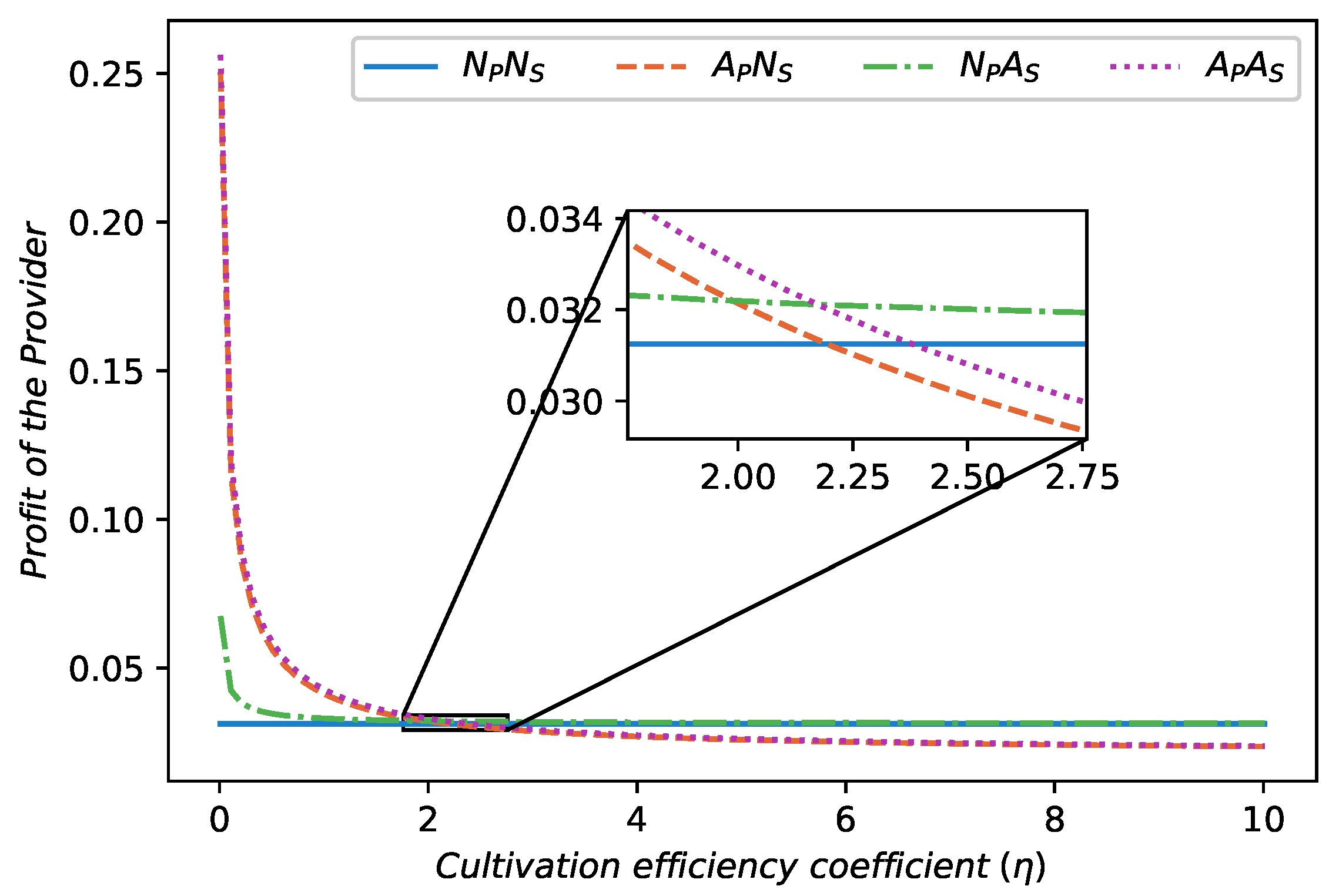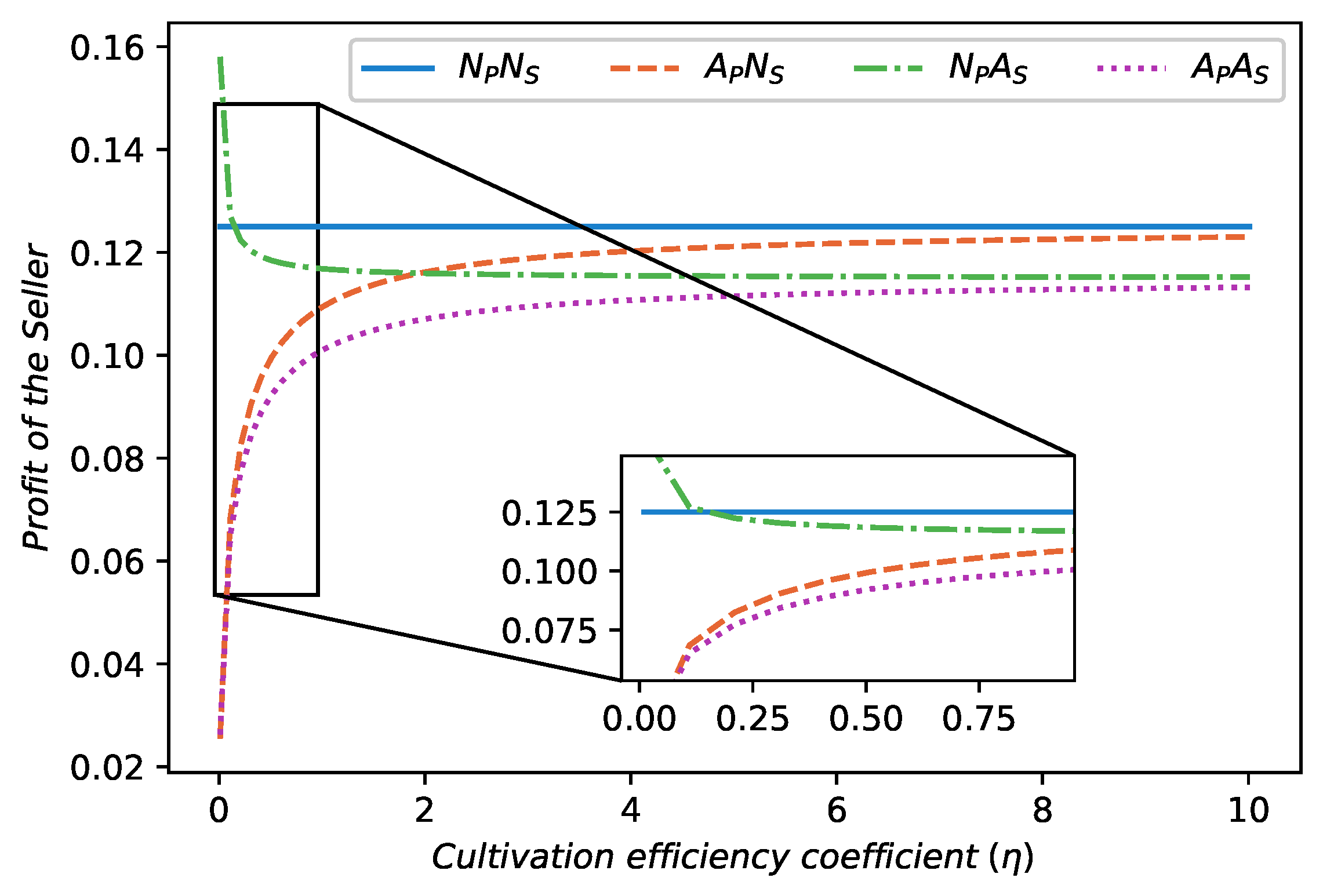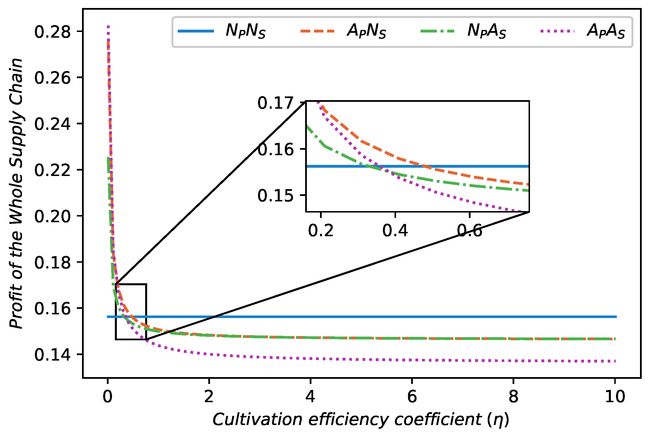According to the above settings, we first obtain the impact of the changes in the cultivation efficiency coefficient on the profits of the provider, the seller, and the whole supply chain in all cases, as shown in Figure 1, Figure 2 and Figure 3. From the three figures, two observations are obtained.

Observation 1.

Given proper F and $\gamma$, the results of the equilibrium live-streaming adoption strategy configurations are as follows:

(i) If $\eta$ is relatively small, both the provider and the seller prefer to adopt live-streaming channels (i.e., $A_P{A}_S$);

(ii) If $\eta$ is relatively medium, the provider prefers to adopt a live-streaming channel, whereas the seller prefers not to (i.e., $A_P{N}_S$);

(iii) If $\eta$ is relatively large, neither the provider nor the seller prefer to adopt live-streaming channels (i.e., $N_P{N}_S$).

Observation 1 reveals that, firstly, if the cultivation efficiency is relatively high (i.e., $\eta$ is relatively small, e.g., from 0 to around $0.12$), adopting a live-streaming channel (i.e., A) is the dominant strategy for both the provider and the seller. This is because, on the one hand, the provider needs to leverage it as a powerful tool to weaken their own disadvantages by threatening the powerful downstream seller and extracting more margins by expanding a new directly accessed market. On the other hand, the seller also needs to introduce it to boost sales or offset the adverse impacts on them brought about by the upstream provider’s opening of the live-streaming channel by strengthening their own attractiveness to the provider. As a result, $A_P{A}_S$ emerges as the equilibrium outcome.

Then, as the cultivation efficiency is reduced to a relatively medium level (i.e., $\eta$ is relatively medium, e.g., from around $0.12$ to around $2.2$), the provider and the seller take different actions. Specifically, adopting a live-streaming channel remains a powerful means and a dominant strategy for the provider to improve their unfavorable position. However, for the seller, introducing a live-streaming channel would, on the contrary, put it in an unfavorable position and cause additional losses. This is due to the increase in the cost of cultivating the potential market size of the live-streaming channel and the diseconomies of the supply scale of the upstream provider. At this time, more products are still sold through channel T with low margins, and the revenues from the live-streaming channel are hardly sufficient to cover the total costs of opening and developing this channel. As a result, $A_P{N}_S$ emerges as the equilibrium outcome.

Finally, when the cultivation efficiency is relatively low (i.e., $\eta$ is relatively large, e.g., around $2.2$ and above), not adopting a live-streaming channel (i.e., N) is the dominant strategy for both the provider and the seller. This is because, for either the provider or the seller, introducing live-streaming channels is an uneconomical practice due to the high related cost. As a result, $N_P{N}_S$ emerges as the equilibrium outcome.

Observation 2.

Compared with the basic case (i.e., $N_P{N}_S$), the impacts of the equilibrium live-streaming adoption strategy configuration on the profits of the provider, the seller, and the whole supply chain are as follows:

(i) If $A_P{A}_S$ emerges, this strategy configuration always benefits the provider and the whole supply chain, while it hurts the seller;

(ii) If $A_P{N}_S$ emerges, this strategy configuration always benefits the provider and hurts the seller, but it may be beneficial or harmful for the whole supply chain;

(iii) If $N_P{N}_S$ emerges, this strategy configuration brings no changes for any members.

Observation 2 reveals that, overall, live streaming is a powerful tool for a weak upstream provider to reverse their disadvantages. However, for a powerful downstream seller, it is more of a means of mitigating the adverse effects brought about by the strategy of the upstream provider. Therefore, among the three equilibrium outcomes, the provider ultimately benefits, while the seller suffers losses. The only difference lies in the degree. In addition, the whole supply chain always benefits from activities when both upstream and downstream members open live-streaming channels simultaneously. However, when only the upstream provider introduces a live-streaming channel; for the whole supply chain to benefit, the cultivation efficiency must not be too low or even at a medium level.

Compared with previous studies that considered the live-streaming adoption strategies of both upstream providers and downstream sellers (e.g., [33,34,35,36]), firstly, similar equilibrium strategy results were obtained, showing that, sometimes, introducing live streaming is dominant, or choice inconsistency emerges between providers and sellers. However, in the downstream-dominant structure, a win–win outcome will not occur in equilibrium, which is quite different from previous findings. This is because, in this structure, a win–win situation will only occur when only the downstream seller adopts live streaming (i.e., $N_P{A}_S$). However, if the seller does so, the provider will quickly adopt a consistent strategy, thereby undermining the emergence of this win–win situation under equilibrium conditions.

6. Conclusions

6.1. Main Findings

This study investigated the live-streaming adoption strategies of providers and sellers within a downstream-dominant supply chain framework. The seller is powerful and controls the procurement price of upstream products while, in contrast, the provider is weak and acts as a price taker. To improve the current situation and expand into new markets, both the provider and the seller are likely to establish their own live-streaming channels. Then, there are four cases regarding the adoption of live-streaming channels, namely, neither party introduces them, only the provider does, only the seller does, or both parties do. Additionally, the live-streaming channel is assumed to possess the characteristics of independence and a potential market that can be endogenized. By deriving the optimal equilibrium results in different cases and comparing them, the live-streaming adoption strategies of both the provider and the seller are discussed, as is the impact of live streaming.

The main findings show that adopting a live-streaming channel is a dominant strategy for both the upstream provider and the downstream seller if it is easy to cultivate the potential market size (i.e., fan base) in newly opened live-streaming channels. However, as the cultivation efficiency declines, the seller will withdraw first, followed by the provider. Compared with the seller, the provider is more likely to benefit from live streaming as they can use it as a means of sending a supply threat signal to the downstream seller and improving their own bottom line. This will relieve the originally weak situation of the provider to a certain extent. However, the live streaming of the seller is restricted by the diseconomies of supply of the weak upstream provider, making it difficult for them to achieve the expected positive effects.

Regarding the impacts of live streaming, on one hand, it can be found that in equilibrium and compared with the basic situation (i.e., neither party introduces live-streaming channels), live streaming always benefits the provider but hurts the seller. It is difficult to achieve a win–win outcome. On the other hand, if the cultivation efficiency is relatively high, both parties introduce live-streaming channels, which can raise the profit of the whole supply chain. In contrast, if the cultivation efficiency is relatively moderate, only the provider introduces a live-streaming channel, and the impact thereof on the profit of the whole supply chain is uncertain. This further depends on whether the cultivation efficiency tends towards the upper bound or the lower bound of the moderate range. Moreover, no matter who introduces the live-streaming channel(s), the procurement and retail prices in the traditional channels will increase over the previous prices. Meanwhile, the retail price in the newly opened live-streaming channel is different from (or consistent with) the current retail price in the traditional channel if it is introduced by the provider (or seller).

6.2. Managerial Implications

These findings have several managerial implications. First, it is crucial to recognize that live-streaming markets, particularly in regions such as China, are evolving rapidly. These markets are transitioning from a phase of rapid growth and expansion to a more mature and competitive state. This shift is characterized by a significant increase in the costs associated with acquiring and retaining loyal fans. Maintaining audience engagement and loyalty has become increasingly challenging, which is primarily due to the high fees required for various traffic promotion services and the difficulty in sustaining viewer interest over time. Consequently, entering the live-streaming market without a strategic plan may not be advantageous for either upstream providers or downstream sellers. This is especially true for upstream providers, who might view live streaming as a potential solution to alleviate their disadvantaged market positions. However, the high costs and competitive nature of the market suggest that a more cautious approach is necessary. In contrast, the live-streaming industry in some emerging markets is still in its early stages of development, presenting more favorable opportunities for entry. For instance, small product providers in China, such as those in the Yiwu area of Zhejiang, have begun to leverage live streaming for cross-border trade. This initiative aligns with the broader context of the One Belt One Road initiative, which encourages economic collaboration and trade expansion. By tapping into these emerging markets, businesses can potentially avoid the intense competition and high costs associated with more established markets while also capitalizing on the growing demand for live-streaming content.

Second, live-streaming platforms should carefully consider their support strategies for top and well-known streamers; while it is natural for platforms to want to promote their most successful and popular streamers, over-investing in these individuals can exacerbate the Matthew effect within the industry. To counteract this, platforms should focus on fostering a more balanced ecosystem that encourages the growth of new talent. By providing targeted support and resources to emerging streamers, platforms can help to level the playing field and promote a healthier market dynamic. Additionally, platforms should tailor their traffic promotion mechanisms and paid services to the specific needs and circumstances of each merchant on the supply side. A one-size-fits-all approach may not be effective, as it can lead to a situation where inferior offerings displace superior ones in the market. By customizing their services, platforms can better support a diverse range of merchants and contribute to a more vibrant and competitive live-streaming environment.

Third, in supply chains where downstream sellers hold significant power, the introduction of live-streaming channels by upstream providers can often result in losses for the dominant downstream sellers. Even if these downstream sellers attempt to mitigate the impact by introducing their own live-streaming channels, they may still struggle to reverse the overall trend of losses. In such cases, a strategic alternative could be for downstream sellers to abandon the idea of opening their own live-streaming channels and instead focus on integrating into the live-streaming operations of upstream providers. By doing so, they can leverage the existing infrastructure and resources of the upstream providers, potentially leading to a more efficient and effective use of resources. To achieve a win–win situation, both parties can explore reasonable benefit-sharing mechanisms. This approach not only allows downstream sellers to participate in the growing live-streaming market but also provides upstream providers with valuable insights into consumer preferences and market trends, ultimately benefiting both parties in the long run.

6.3. Limitations and Future Study

Although this study focuses on discussing the live-streaming adoption strategies of each member in downstream-dominant supply chains and the impacts of live-streaming, there are still some limitations that can be further explored in the future. First, this study takes into account a simple supply chain structure composed of a single provider and a single seller. However, the situation of multiple providers and/or sellers also deserves to be discussed further. Providers can be differentiated, and so can sellers. In this way, more complex but more realistic scenarios can be depicted, such as competitive situations among multiple live-streaming platform giants (e.g., TikTok, Kwai, JD Live, and Taobao Live) with numerous individuals participating. Then, more in-depth and detailed issues will be explored, such as the problem of the level of heterogeneity or homogeneity of live-streaming strategies in the live-streaming market.

Second, the factor of competition among supply chains deserves further consideration. This may also be an important driving force for promoting live streaming to enter the original and traditional supply chains. This triggers a series of questions. For example, when introducing live streaming, will this change the competitive landscape of the supply chain? Will this change the cooperation modes within and between supply chains? Will this change the channel power structure dominated by the downstream? Especially when downstream live-streaming platforms and streamers are playing an increasingly important role, the downstream-dominated attribute of a live-streaming channel is also quite prominent and is very likely to be different from the downstream-dominated characteristics in the traditional supply chain. As a result, the cross-linking and mutual influence among different channels, different supply chains, and different power structures impact product sales and the operation of supply chains; all of these considerations are worthy of further exploration.

Third, in this study, it is considered that the provider, the seller, and consumers are rational. However, some behavioral factors of decision-makers could be further explored. Especially in real live-streaming scenarios, there are numerous small individual decision-makers, who are more likely to exhibit certain behaviors. Examples include consumers’ herd behavior and impulsive consumption behavior, as well as the speculative behaviors of streamers and merchants.

References

1. It’s Showtime! How Live Commerce is Transforming the Shopping Experience. Available online: https://www.mckinsey.com/capabilities/mckinsey-digital/our-insights/its-showtime-how-live-commerce-is-transforming-the-shopping-experience (accessed on 21 July 2021).
2. Live Commerce-Statistics & Facts. Available online: https://www.statista.com/topics/8752/livestream-commerce/#topicOverview (accessed on 5 April 2024).
3. Live Commerce: Top Chinese Platforms, Revenue & Market Analysis. Available online: https://ecommercedb.com/insights/livestream-commerce-in-china-taobao-leads-but-its-dominance-fades/4598 (accessed on 26 September 2024).
4. Gen Z Livestream E-Commerce Participation and Awareness 2023, by Country. Available online: https://www.statista.com/statistics/1395802/gen-z-livestream-shopping-by-country/ (accessed on 1 June 2023).
5. Breakdown of Traditional E-Commerce and Live Commerce Users China 2021, by Generation. Available online: https://www.statista.com/statistics/1284686/china-age-breakdown-of-traditional-and-livestreaming-e-commerce-users/ (accessed on 1 January 2022).
6. Liu, Z.L.; Li, J.N.; Wang, X.Q.; Guo, Y.R. How search and evaluation cues influence consumers’ continuous watching and purchase intentions: An investigation of live-stream shopping from an information foraging perspective. J. Bus. Res. 2023, 168, 114233. [Google Scholar] [CrossRef]
7. Ma, X.Y.; Chen, H.Z.; Lang, X.P.; Li, T.S.; Wu, N.W.; Duong, B. Research on the impact of streamers’ linguistic emotional valence on live streaming performance in live streaming shopping environments. J. Retail. Consum. Serv. 2024, 81, 104040. [Google Scholar] [CrossRef]
8. Tian, Y.; Frank, B. Optimizing live streaming features to enhance customer immersion and engagement: A comparative study of live streaming genres in China. J. Retail. Consum. Serv. 2024, 81, 103974. [Google Scholar] [CrossRef]
9. Choi, Y.S.; Wu, Q.Q.; Lee, J.Y. Can you tolerate influencer marketing? An empirical investigation of live streaming viewership reduction related to influencer marketing. J. Bus. Res. 2025, 188, 115094. [Google Scholar] [CrossRef]
10. Pan, R.; Feng, J.; Zhao, Z.L. Fly with the wings of live-stream selling-channel strategies with/without switching demand. Prod. Oper. Manag. 2022, 31, 3387–3399. [Google Scholar] [CrossRef]
11. Wang, S.S.; Guo, X. Strategic cooperation of live-stream platform in e-commerce. Manag. Decis. Econ. 2023, 44, 4201–4227. [Google Scholar] [CrossRef]
12. Chen, L.D.; Xu, Q.Y.; He, Y. Channel selection strategy with consumer impulse purchase in livestream selling. Manag. Decis. Econ. 2024, 45, 5006–5019. [Google Scholar] [CrossRef]
13. Zhang, W.; Yu, L.L.; Wang, Z.Z. Live-streaming selling modes on a retail platform. Transport. Res. E-Log. 2023, 173, 103096. [Google Scholar] [CrossRef]
14. Duan, Y.R.; Song, J. The adoption of live streaming channel considering impulse buying and product returns. Int. J. Prod. Econ. 2024, 274, 109295. [Google Scholar] [CrossRef]
15. Liu, Z.; Chen, H.R.; Zhang, X.M.; Gajpal, Y.; Zhang, Z.C. Optimal channel strategy for an e-seller: Whether and when to introduce live streaming? Electron. Commer. Res. Appl. 2024, 63, 101348. [Google Scholar] [CrossRef]
16. Zhang, T.; Tian, Y.; Cheng, T.C.E. Online Retailing with Key Opinion Leaders and Product Returns. Int. J. Prod. Econ. 2024, 1–30. Available online: https://www.sciencedirect.com/science/article/abs/pii/S0925527324003153?via%3Dihub (accessed on 1 November 2024). [CrossRef]
17. Zhang, Y.F.; Xu, Q. Consumer engagement in live streaming commerce: Value co-creation and incentive mechanisms. J. Retail. Consum. Serv. 2024, 81, 103987. [Google Scholar] [CrossRef]
18. Li, K.L.; Yao, S.; Li, Y.J.; Tang, F.C.; Wang, Z.B. Deliberate shortage in live-streaming commerce. Omega 2025, 131, 103201. [Google Scholar] [CrossRef]
19. Zhang, T.; Tang, Z.J. Should manufacturers open live streaming shopping channels? J. Retail. Consum. Serv. 2023, 71, 103229. [Google Scholar] [CrossRef]
20. Li, Y.R.; Li, B.; Wang, M.X.; Liu, Y. Optimal sales strategies for an omni-channel manufacturer in livestreaming demonstration trends. Transport. Res. E-Log. 2023, 180, 103222. [Google Scholar] [CrossRef]
21. Wang, X.T.; Han, X.H.; Chen, Y. Optimal manufacturer strategy for live-stream selling and product quality. Electron. Commer. Res. Appl. 2024, 64, 101372. [Google Scholar] [CrossRef]
22. Zhao, Q.L.; Fan, Z.P. Two-period pricing of an e-tailer: Is using a top influencer to promote new products a bane or a boon? Electron. Commer. Res. Appl. 2024, 63, 101345. [Google Scholar] [CrossRef]
23. Gong, H.Y.; Zhao, M.; Ren, J.L.; Hao, Z.H. Live streaming strategy under multi-channel sales of the online retailer. Electron. Commer. Res. Appl. 2022, 55, 101184. [Google Scholar] [CrossRef]
24. Xu, Q.Y.; Shao, Z.; Zhang, L.; He, Y. Optimal livestream selling strategy with buy-online-and-return-in-store. Electron. Commer. Res. Appl. 2023, 61, 101307. [Google Scholar] [CrossRef]
25. Liu, X.F.; Zhou, Z.B.; Hu, M.H.; Zhong, F.M. How retailers can gain more profitability driven by digital technology: Live streaming promotion and blockchain technology traceability? Electron. Commer. Res. Appl. 2024, 68, 101445. [Google Scholar] [CrossRef]
26. Fan, X.J.; Zhang, L.; Guo, X.; Zhao, W.Y. The impact of live-streaming interactivity on live-streaming sales mode based on game-theoretic analysis. J. Retail. Consum. Serv. 2024, 81, 103981. [Google Scholar] [CrossRef]
27. Lu, W.; Ji, X.; Wu, J. Retailer’s information sharing and manufacturer’s channel expansion in the live-streaming e-commerce era. Eur. J. Oper. Res. 2025, 320, 527–543. [Google Scholar] [CrossRef]
28. Niu, B.Z.; Yu, X.H.; Li, Q.Y.; Wang, Y.L. Gains and losses of key opinion leaders’ product promotion in livestream e-commerce. Omega 2023, 117, 102846. [Google Scholar] [CrossRef]
29. Zhang, T.; Tang, Z.J.; Han, Z.Y. Optimal online channel structure for multinational firms considering live streaming shopping. Electron. Commer. Res. Appl. 2022, 56, 101198. [Google Scholar] [CrossRef]
30. Zhang, Y.F.; Xu, Q. Whether and how to adopt live streaming selling: A perspective on interaction value creation. Electron. Commer. Res. Appl. 2024, 68, 101464. [Google Scholar] [CrossRef]
31. Chen, Q.Y.; Yan, X.; Zhao, Y.; Bian, Y.W. Live streaming channel strategy of an online retailer in a supply chain. Electron. Commer. Res. Appl. 2023, 62, 101321. [Google Scholar] [CrossRef]
32. Chen, Q.Y.; Yan, X.; Bian, Y.W.; Han, X.H. Live streaming channel and product assortment with both national and store brand products. Omega 2025, 131, 103212. [Google Scholar] [CrossRef]
33. Cui, X.Q.; Li, Y.J.; Li, X.; Fang, S.L. Livestream e-commerce in a platform supply chain: A product-fit uncertainty reduction perspective. Int. J. Prod. Econ. 2023, 258, 108796. [Google Scholar] [CrossRef]
34. Ji, G.J.; Fu, T.Y.; Li, S.H. Optimal selling format considering price discount strategy in live-streaming commerce. Eur. J. Oper. Res. 2023, 309, 529–544. [Google Scholar] [CrossRef]
35. Yang, W.T.; Govindan, K.; Zhang, J.T. Spillover effects of live streaming selling in a dual-channel supply chain. Transport. Res. E-Log. 2023, 180, 103298. [Google Scholar] [CrossRef]
36. Wang, S.S.; Guo, X. Strategic introduction of live-stream selling in a supply chain. Electron. Commer. Res. Appl. 2023, 62, 101315. [Google Scholar] [CrossRef]
37. Huang, L.C.; Liu, B.; Zhang, R. Channel strategies for competing retailers: Whether and when to introduce live stream? Eur. J. Oper. Res. 2024, 312, 413–426. [Google Scholar] [CrossRef]
38. Niu, B.Z.; Chen, Y.Y.; Zhang, J.H.; Chen, K.L.; Jin, Y. Brands’ livestream selling with influencers’ converting fans into consumers. Omega 2025, 131, 103195. [Google Scholar] [CrossRef]
39. Lu, Y.S.; Duan, Y.R. Strategic live streaming choices for vertically differentiated products. J. Retail. Consum. Serv. 2024, 76, 103582. [Google Scholar] [CrossRef]
40. Li, Z.W.; Liu, D.S.; Zhang, J.K.; Wang, P.; Guan, X. Live streaming selling strategies of online retailers with spillover effects. Electron. Commer. Res. Appl. 2024, 63, 101330. [Google Scholar] [CrossRef]
41. Xin, B.G.; Hao, Y.R.; Xie, L. Strategic product showcasing mode of e-commerce live streaming. J. Retail. Consum. Serv. 2023, 73, 103360. [Google Scholar] [CrossRef]
42. Jin, D.L.; Lai, D.L.; Pu, X.J.; Han, G.H. Self-broadcasting or cooperating with streamers? A perspective on live streaming sales of fresh products. Electron. Commer. Res. Appl. 2024, 64, 101367. [Google Scholar] [CrossRef]
43. Liu, B.L.; Wang, W.L. Live commerce retailing with online influencers: Two business models. Int. J. Prod. Econ. 2023, 255, 108715. [Google Scholar] [CrossRef]
44. Mao, Z.F.; Du, Z.L.; Yuan, R.Y.; Miao, Q.Q. Short-term or long-term cooperation between retailer and MCN? New launched products sales strategies in live streaming e-commerce. J. Retail. Consum. Serv. 2022, 67, 102996. [Google Scholar] [CrossRef]
45. Du, Z.; Fan, Z.P.; Sun, F.H. Live streaming sales: Streamer type choice and limited sales strategy for a manufacturer. Electron. Commer. Res. Appl. 2023, 61, 101300. [Google Scholar] [CrossRef]
46. Ye, F.; Ji, L.; Ning, Y.; Li, Y.N. Influencer selection and strategic analysis for live streaming selling. J. Retail. Consum. Serv. 2024, 77, 103673. [Google Scholar] [CrossRef]
47. Hao, C.X.; Yang, L. Resale or agency sale? Equilibrium analysis on the role of live streaming selling. Eur. J. Oper. Res. 2023, 307, 1117–1134. [Google Scholar] [CrossRef]
48. Xu, X.P.; Yang, Y.Y.; Zhang, J.Z.; Cheng, T.C.E. Live streaming platform operations and coordination under the cap-and-trade regulation: Platform-enabled mode versus platform-agency mode. Int. J. Prod. Econ. 2023, 260, 108859. [Google Scholar] [CrossRef]
49. Niu, B.Z.; Yu, X.H.; Dong, J. Could AI livestream perform better than KOL in cross-border operations? Transport. Res. E-Log. 2023, 174, 103130. [Google Scholar] [CrossRef]
50. Xu, X.P.; Wang, Y.T.; Cheng, T.C.E.; Choi, T.M. Should live broadcasting platforms adopt artificial intelligence? A sales effort perspective. Eur. J. Oper. Res. 2024, 318, 979–999. [Google Scholar] [CrossRef]
51. Liu, X.F.; Zhou, Z.B.; Zhong, F.M.; Hu, M.H. Resolving the information reliability issue in live streaming through blockchain adoption. Transport. Res. E-Log. 2024, 189, 103652. [Google Scholar] [CrossRef]
52. Li, G.; Li, X.C.; Zheng, H. Discount preannouncement in the digital supply chain era. Int. J. Prod. Econ. 2023, 258, 108815. [Google Scholar] [CrossRef]
53. Zhou, C.; Yu, J.; Qian, Y. Should live-streaming platforms nonexclusively promote brands from traditional retail platforms? J. Retail. Consum. Serv. 2024, 80, 103930. [Google Scholar] [CrossRef]
54. Zhen, X.P.; Wang, P.; Li, X.R. The Streamer’s sales strategy choice considering sales effort. J. Retail. Consum. Serv. 2024, 78, 103745. [Google Scholar] [CrossRef]
55. Xie, L.; Guo, G.T.; Chen, J. Bundling products and service on influencer channels. J. Retail. Consum. Serv. 2024, 79, 103833. [Google Scholar] [CrossRef]
56. Liu, J.Q.; Yuan, R.; Feng, S.; Wang, G.X. Quality-differentiated distribution strategies between live streaming and online channels. J. Retail. Consum. Serv. 2025, 82, 104056. [Google Scholar] [CrossRef]
57. Cheng, Y.W. Live-streaming commerce in the supply chain with equity cooperation: Independent or cooperative? Mathematics 2024, 12, 2334. [Google Scholar] [CrossRef]
58. Zhang, Y.F.; Xu, Q.; Zhang, G.Q. Optimal contracts with moral hazard and adverse selection in a live streaming commerce market. J. Retail. Consum. Serv. 2023, 74, 103419. [Google Scholar] [CrossRef]
59. Li, R.; Huang, W.D. Differential games between a brand manufacturer and an internet celebrity regarding fairness concerns. Mathematics 2024, 12, 3154. [Google Scholar] [CrossRef]
60. Li, J.; Kouvells, P.; Dada, M. Agricultural supply chains in emerging markets: Competition and cooperation under correlated yields. Manuf. Serv. Oper. Manag. 2024, 26, 664–680. [Google Scholar] [CrossRef]
61. Hong, X.P.; He, Y.M.; Zhou, P.; Chen, J.G. Demand information sharing in a contract farming supply chain. Eur. J. Oper. Res. 2023, 309, 560–577. [Google Scholar] [CrossRef]
62. Wang, J.B.; Zhang, T.; Fan, X.J. Reverse channel design with a dominant retailer and upstream competition in emerging markets: Retailer- or manufacturer- collection? Transport. Res. E-Log. 2020, 173, 101924. [Google Scholar] [CrossRef]
63. Zhang, S.C.; Wei, L.Q.; Zhang, J.X. Demand forecast sharing for a dominant retailer with supplier encroachment and quality decisions. Eur. J. Oper. Res. 2022, 301, 39–50. [Google Scholar] [CrossRef]
64. How to Start a Successful Live Streaming Business. Available online: https://stepbystepbusiness.com/business-ideas/start-a-live-streaming-business/#:~:text=How%20much%20does%20it%20cost%20to%20start%20a,include%20a%20computer%2C%20equipment%2C%20and%20a%20marketing%20budget (accessed on 2 June 2023).
Figure 1. Profits of the provider in different cases.
Mathematics 13 00230 g001
Figure 2. Profits of the seller in different cases.
Mathematics 13 00230 g002
Figure 3. Profits of the whole supply chain in different cases.
Mathematics 13 00230 g003