Article

Investigations of Modified Classical Dynamical Models: Melnikov’s Approach, Simulations and Applications, and Probabilistic Control of Perturbations

1
Faculty of Mathematics and Informatics, University of Plovdiv Paisii Hilendarski, 24, Tzar Asen Str., 4000 Plovdiv, Bulgaria
2
Institute of Mathematics and Informatics, Bulgarian Academy of Sciences, Acad. G. Bonchev Str., Bl. 8, 1113 Sofia, Bulgaria
3
Faculty of Mathematics and Informatics, Sofia University “St. Kliment Ohridski”, 5, James Bourchier Blvd., 1164 Sofia, Bulgaria
*
Author to whom correspondence should be addressed.
Mathematics 2025, 13(2), 231; https://doi.org/10.3390/math13020231
Submission received: 9 December 2024 / Revised: 7 January 2025 / Accepted: 9 January 2025 / Published: 11 January 2025

Abstract

:
We suggest a few kinds of extended classical oscillators in this study. We present a few specific modules for examining these oscillators’ behavior. This will be an essential component of a broader web-based scientific computing platform that is in the works. The modeling and synthesis of radiating antenna designs is also taken into consideration as a potential use case for Melnikov functions. Additionally, we discuss strategies for achieving probabilistic control over system perturbations.

1. Introduction

A number of authors have researched the classical differential model:
d x d t = y d y d t = sin x + ϵ F ( x , y ) y ,
where 0 ϵ < 1 . The literature on this subject is extensive and diverse. The outstanding studies of Tricomi [1], Stoker [2], Levi, Hoppensteadt and Miranker [3], Perko [4], and Guckenheimer and Holmes [5] provide the reader with comprehensive information. A universal escape nonlinear oscillator model describes a variety of oscillatory physical phenomena that occur in various fields, including mechanics, quantum optics, acoustics, hydrodynamics, electronics, and engineering. The equation of motion for the sinusoidally driven escape oscillator, which includes nonlinear damping terms as a power series on the velocity, has been examined by Sanjuan [6]. See [7,8,9,10,11,12,13,14] for additional results. We examine the following model in [15].
d x d t = y d y d t = sin x + ϵ a 1 + i = 0 n 2 1 a n 2 i x n 2 i + i = 0 n 2 2 b n 2 2 i y n 2 2 i y ,
where 0 ϵ < 1 and n is even. The classical differential model—the damped mathematical pendulum excited by horizontal harmonics—is the focus of several authors’ studies [16,17,18,19,20,21]:
x ¨ + ϵ δ x ˙ + sin x + ϵ γ cos ( ω t ) cos x = 0
or
d x d t = y d y d t = sin x ϵ ( δ y + γ cos ( ω t ) cos x ) ,
where 0 ϵ < 1 . In this paper, we suggest some classes of extended classical oscillators. Studies are examined in the context of Melnikov’s methodology [22]. We offer several simulations. Additionally, we present a few specialized modules for examining the dynamics of these fictitious oscillators. The obtained results can be included into a much broader scientific computing application—see [23,24,25,26,27,28] for additional information. The following is the paper’s plan. In Section 2.1 and Section 2.2, we provide our models. Section 2.1.1 and Section 2.2.1 examine investigations in the context of Melnikov’s methodology. Section 2.1.2 and Section 2.2.2 contain a few simulations. Section 2.1.3 and Section 2.2.3 address one potential use of Melnikov functions, which is in the modeling of radiating antenna designs. Section 3 brings us to a close. Appendix A and Appendix B provide probabilistic control over the perturbations.

2. The Models

2.1. The Model A

The following novel class of extended oscillators is examined.
d x d t = y d y d t = sin x ϵ A p = 1 n y | y | p 1 j = 1 N g j sin ( j ω t ) ,
where A is the damping level, p 1 is the damping exponent, N is an integer, and 0 ϵ < 1 . Specifically, we take into account the following model:
d x d t = y d y d t = sin x ϵ A y | y | p 1 j = 1 N g j sin ( j ω t ) .
The equation H ( x , y ) = 1 2 y 2 + 1 cos x represents the system’s total energy ( ϵ = 0 ). Some details can be found in monograph [5]. The orbit is provided by (refer to Figure 1):
x 0 ( t ) = ± 2 arctan ( sinh t ) ; y 0 ( t ) = ± 2 sech t .

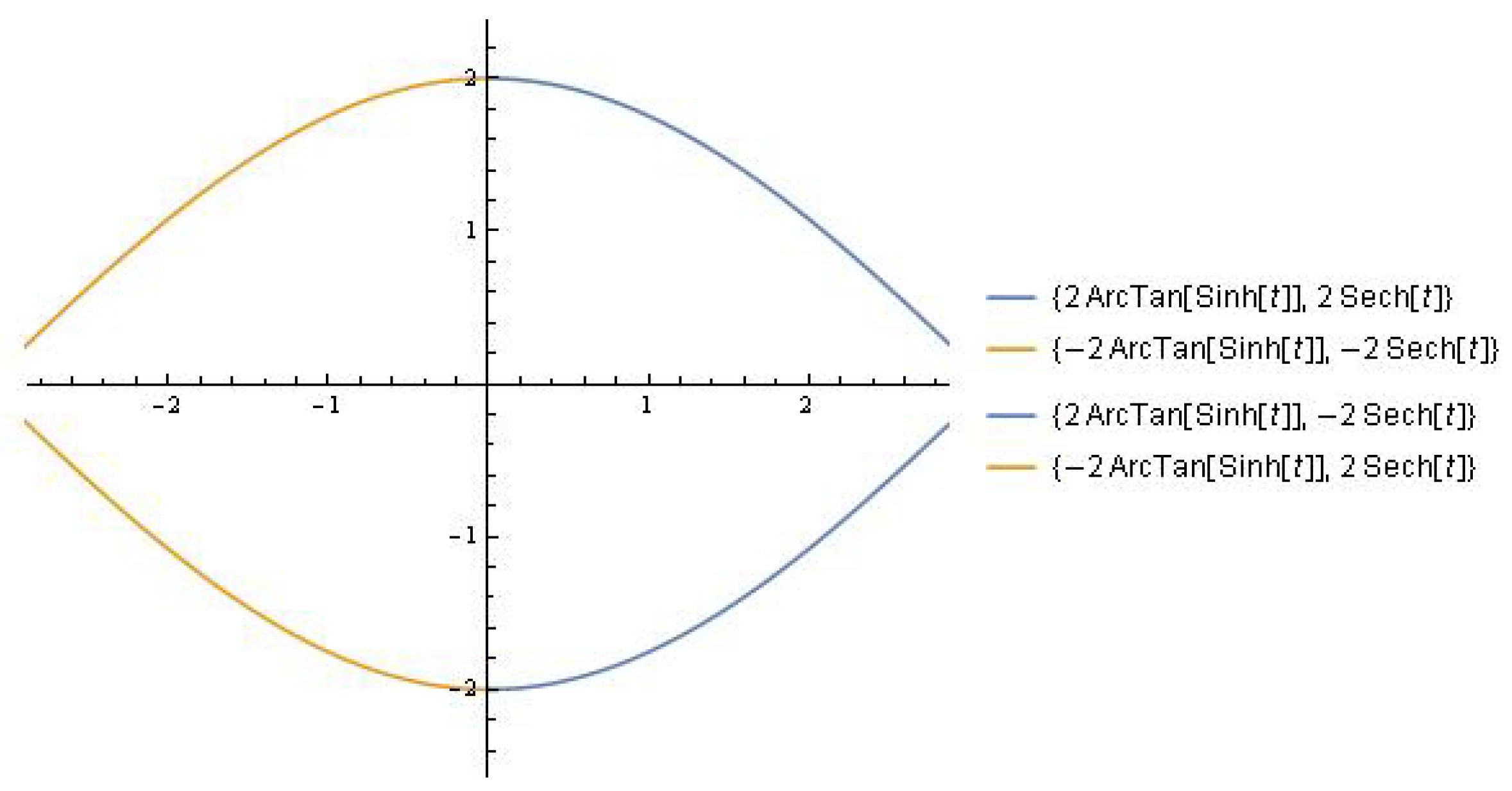
2.1.1. Observations in View of Melnikov’s Methodology

The Melnikov function can be used to determine the transverse intersection of the stable and unstable manifolds and provides a measure of the leading order distance between them when ϵ 0 . By definition, the Melnikov integral is provided by
M ( t 0 ) = y 0 ( t ) A y 0 ( t ) | y 0 ( t ) | p 1 j = 1 N g i sin ( j ω ( t + t 0 ) ) d t ,
where Equation (7) defines the functions x 0 ( t ) and y 0 ( t ) . The task of determining the root of M ( t 0 ) is more intriguing from a numerical perspective as the parameters that appear in the suggested differential model are subject to certain practical and physical constraints.
Proposition 1.
The roots of the Melnikov function M ( t 0 ) are provided as equation solutions if p = 2 and N = 1
M ( t 0 ) = 2 π 2 A g 1 sech π ω 2 sin ( t 0 ω ) = 0 .
M ( t 0 ) = 0 (for p = 2 ; N = 1 ; A = 0.015 ; ω = 0.2 ; g 1 = 0.09 ), for instance, is shown on Figure 2. In the interval ( 0 , 16 ) , the roots are: 1.78742 ; 13.9205 . Melnikov’s condition for chaotic behavior of the dynamical model can be formulated by the reader from Proposition 1 (also see Figure 2).
Proposition 2.
The roots of the Melnikov function M ( t 0 ) are provided as equation solutions for p = 2 and N = 2
M ( t 0 ) = 2 π 2 A g 1 sech π ω 2 sin ( t 0 ω ) g 2 sech ( π ω ) sin ( 2 t 0 ω ) = 0 .
For instance, the formula M ( t 0 ) = 0 is shown in Figure 3 (for p = 2 ; N = 2 ; A = 0.015 ; ω = 0.6 ; g 1 = 0.07 ; g 2 = 0.3 ). The following are the roots in the interval of ( 0 , 10 ) : 0.224036 ; 2.7794 ; 5.63804 ;   7.0665 . We can demonstrate the following claim when p = 4 and N = 1 .
Proposition 3.
The roots of the Melnikov function M ( t 0 ) are provided as equation solutions for p = 4 and N = 1
M ( t 0 ) = 2 π 6 A g 1 sech π ω 2 sin ( t 0 ω ) = 0 .
For instance, Figure 4 shows the equation M ( t 0 ) = 0 (for p = 4 ; N = 1 ; A = 0.015 ; ω = 0.1 ; g 1 = 0.091 ). The root in interval ( 0 , 16 ) is: 15.708 with a multiplicity of two.
Proposition 4.
The roots of the Melnikov function M ( t 0 ) are provided as equation solutions for p = 4 and N = 2
M ( t 0 ) = 2 π 6 A g 1 sech π ω 2 sin ( t 0 ω ) g 2 sech ( π ω ) sin ( 2 t 0 ω ) = 0 .
As an illustration, Figure 5 shows the equation M ( t 0 ) = 0 (for p = 4 ; N = 2 ; A = 0.011 ; ω = 0.92 ; g 1 = 0.091 ; g 2 = 0.32 ). The roots (with a multiplicity of two) at an interval of ( 0 , 10 ) are: 0.97718 ; 7.92402 . M ( t 0 ) = 0 is the equation (for p = 4 ; N = 2 ; A = 0.02 ; ω = 0.7 ; g 1 = 0.005 ; g 2 = 0.2 ) and has no roots (see Figure 6).
Proposition 5.
The roots of the Melnikov function M ( t 0 ) are provided as equation solutions if p = 4 and N = 3
M ( t 0 ) = 1 1 + 2 cosh ( π ω ) e 2 i t 0 ω π i e 2 i t 0 ω g 1 + i e 4 i t 0 ω g 1 + 6 A e 2 i t 0 ω cosh π ω 2 + i e 2 i t 0 ω g 1 cosh ( π ω ) i e 4 i t 0 ω g 1 cosh ( π ω ) i g 3 cosh ( π ω ) + i e 6 i t 0 ω g 3 cosh ( π ω ) i e i t 0 ω g 2 cosh 3 π ω 2 + i e 5 i t 0 ω g 2 cosh 3 π ω 2 i e 2 i t 0 ω g 1 cosh ( 2 π ω ) + i e 4 i t 0 ω g 1 cosh ( 2 π ω ) + 6 A e 3 i t 0 ω cosh 5 π ω 2 sech π ω 2 sech ( π ω ) = 0 .
For instance, the equation M ( t 0 ) = 0 (for p = 4 ; N = 3 ; A = 0.05 ; ω = 0.09 ; g 1 = 0.6 ; g 2 = 0.3 ; g 3 = 0.1 ) is depicted on Figure 7.
Proposition 6.
The roots of the Melnikov function M ( t 0 ) are provided as equation solutions if p = 6 and N = 2
M ( t 0 ) = 2 π 20 A g 1 sech π ω 2 sin ( t 0 ω ) g 2 sech ( π ω ) sin ( 2 t 0 ω ) = 0 .
Melnikov’s criterion for the occurrence of the intersection between the perturbed and unperturbed separatrixes can be formulated by the reader using Propositions 1 through 6. The analogous approximation issue for randomly selected p and N can be examined by the reader.

2.1.2. Some Simulations

We will concentrate on a few interesting simulations here:
1. For the given p = 2 ; N = 2 ; A = 0.015 ; ϵ = 0.1 ; ω = 0.6 ; g 1 = 0.07 ; g 2 = 0.3 , the simulations on the system (6) for x 0 = 0.6 ; y 0 = 0.2 are depicted in Figure 8.
2. For the given p = 4 ; N = 2 ; A = 0.011 ; ϵ = 0.1 ; ω = 0.92 ; g 1 = 0.9 ; g 2 = 0.2 , the simulations on the system (6) for x 0 = 0.7 ; y 0 = 0.3 are depicted in Figure 9.
3. For the given p = 6 ; N = 3 ; A = 0.011 ; ϵ = 0.1 ; ω = 0.98 ; g 1 = 0.96 ; g 2 = 0.1 ; g 3 = 0.6 , the simulations on the system (6) for x 0 = 0.8 ; y 0 = 0.4 are depicted in Figure 10.

2.1.3. The Modeling and Synthesis of Radiating Antenna Patterns Is One Potential Use for Melnikov Functions

This brings us to M ( t ) . The hypothetical normalized antenna factor is defined as follows: The formula is M ( θ ) = 1 D | M ( K cos θ + k 1 ) | , where θ is the azimuth angle, K = k d ;   k = 2 π λ ; λ is the wave length, d is the distance between emitters, and k 1 is the phase difference.
For fixed A = 0.0001 ; ω = 0.27 ; g 1 = 0.6 ; g 2 = 0.001 ; K = 19.91 ; k 1 = 0.001 (from Proposition 4), see Figure 11.
For fixed A = 0.002 ; ω = 0.27 ; g 1 = 0.07 ; g 2 = 0.001 ; K = 20.91 ; k 1 = 0 (from Proposition 6), see Figure 12.
Naturally, the hypothetical Melnikov array that we provided can be viewed as an addition to the Array Antenna Theory, following careful evaluation by experts in this field of study.

2.2. The Model B

The following novel class of extended oscillators is examined
d x d t = y d y d t = sin x ϵ A p = 1 n y | y | p 1 + cos x j = 1 N g j cos ( j ω t ) ,
where A is the damping level, p 1 is the damping exponent, N is an integer, and 0 ϵ < 1 . Specifically, we take into account the following model
d x d t = y d y d t = sin x ϵ A y | y | p 1 + cos x j = 1 N g j cos ( j ω t ) .

2.2.1. Taking into Account Melnikov’s Methodology

The integral of Melnikov is defined as follows
M ( t 0 ) = y 0 ( t ) A y 0 ( t ) | y 0 ( t ) | p 1 + cos ( x 0 ( t ) ) j = 1 N g i cos ( j ω ( t + t 0 ) ) d t ,
where Equation (7) defines the functions x 0 ( t ) and y 0 ( t ) .
Proposition 7.
The roots of the Melnikov function M ( t 0 ) are provided as equation solutions if p = 2 and N = 1
M ( t 0 ) = 2 π 2 A + g 1 ω 2 cos ( t 0 ω ) sech π ω 2 = 0 .
As an illustration, the equation M ( t 0 ) = 0 (for p = 2 ; N = 1 ; A = 0.0025 ; ω = 0.3 ;   g 1 = 0.17 ) is depicted in Figure 13. The roots in at an interval of ( 0 , 20 ) are: 6.47699 ; 14.467 .
The reader can derive Melnikov’s condition for the dynamical model’s chaotic behavior from Proposition 7 (also see Figure 13).
Proposition 8.
The roots of the Melnikov function M ( t 0 ) are provided as equation solutions for p = 4 and N = 2
M ( t 0 ) = 2 π 6 A + g 1 ω 2 cos ( t 0 ω ) sech π ω 2 + 4 g 2 ω 2 cos ( 2 t 0 ω ) sech ( π ω ) = 0 .
As an illustration, the equation M ( t 0 ) = 0 (for p = 4 ; N = 2 ; A = 0.0025 ; ω = 0.4 ; g 1 = 0.17 ; g 2 = 0.05 ) is depicted in Figure 14. The root in interval ( 0 , 5 ) is: 3.74239 .
Proposition 9.
The roots of the Melnikov function M ( t 0 ) are provided as equation solutions if p = 6 and N = 3
M ( t 0 ) = 2 π 20 A + g 1 ω 2 cos ( t 0 ω ) sech π ω 2 + 4 g 2 ω 2 cos ( 2 t 0 ω ) sech ( π ω ) + 9 g 3 ω 2 cos ( 3 t 0 ω ) sech 3 π ω 2 = 0 .
As an illustration, the equation M ( t 0 ) = 0 (for p = 6 ; N = 3 ; A = 0.001 ; ω = 0.7 ;   g 1 = 0.1 ; g 2 = 0.05 ; g 3 = 0.01 ) has a root of 2.15038 (in interval ( 0 , 3 ) (see Figure 15).
For p = 6 ; N = 3 ; A = 0.001 ; ω = 0.35 ; g 1 = 0.08 ; g 2 = 0.06 ; g 3 = 0.01 , the equation M ( t 0 ) = 0 has no roots (see Figure 16).

2.2.2. Some Simulations

We will concentrate on a few interesting simulations here:
1. For the given p = 4 ; N = 2 ; A = 0.015 ; ϵ = 0.01 ; ω = 0.6 ; g 1 = 0.07 ; g 2 = 0.3 , the simulations on the system (5.16) for x 0 = 0.6 ; y 0 = 0.3 are depicted in Figure 17.
2. For the given p = 6 ; N = 3 ; A = 0.005 ; ϵ = 0.01 ; ω = 0.3 ; g 1 = 0.07 ; g 2 = 0.3 ; g 3 = 0.5 , the simulations on the system (5.16) for x 0 = 0.7 ; y 0 = 0.4 are depicted in Figure 18.

2.2.3. The Modeling and Synthesis of Radiating Antenna Patterns Is One Potential Use for Melnikov Functions (See Section 2.1.3 for Additional Information)

For fixed A = 0.0025 ; ω = 0.4 ; g 1 = 0.17 ; g 2 = 0.05 ; K = 6 ; k 1 = 0.1 (from Proposition 8), see Figure 19.
For fixed A = 0.001 ; ω = 0.6 ; g 1 = 0.16 ; g 2 = 0.1 ; g 3 = 0.01 ; K = 3.44 ; k 1 = 0.01 (from Proposition 9), see Figure 20.
For arbitrarily selected p and N, the reader can examine the corresponding approximation problem.
Proposition 10.
The roots of the Melnikov function M ( t 0 ) are provided as solutions to the following equation if p = 8 and N = 4
M ( t 0 ) = 2 π 70 A + g 1 ω 2 cos ( t 0 ω ) sech π ω 2 + 4 g 2 ω 2 cos ( 2 t 0 ω ) sech ( π ω ) + 9 g 3 ω 2 cos ( 3 t 0 ω ) sech 3 π ω 2 + 16 g 4 ω 2 cos ( 4 t 0 ω ) sech ( 2 π ω ) = 0 .
As an illustration, equation M ( t 0 ) = 0 (for p = 8 ; N = 4 ; A = 0.0001 ; ω = 0.95 ; g 1 = 0.1 ; g 2 = 0.03 ; g 3 = 0.2 ; g 4 = 0.05 ) is depicted in Figure 21).
For p = 8 ; N = 4 ; A = 0.001 ; ω = 0.4 ; g 1 = 0.1 ; g 2 = 0.03 ; g 3 = 0.1 ; g 4 = 0.05 ), equation M ( t 0 ) = 0 has no roots (see Figure 22).
The potential normalized antenna factor M ( θ ) in the case p = 8 ; N = 4 and fixed A = 0.0001 ; ω = 0.95 ; g 1 = 0.1 ; g 2 = 0.03 ; g 3 = 0.2 ; g 4 = 0.05 ; K = 3.44 ; k 1 = 0.1 (from Proposition 10), see Figure 23.
Proposition 11.
The roots of the Melnikov function M ( t 0 ) are provided as equation solutions if p = 10 and N = 6
M ( t 0 ) = 2 π 252 A + g 1 ω 2 cos ( t 0 ω ) sech π ω 2 + 4 g 2 ω 2 cos ( 2 t 0 ω ) sech ( π ω ) + 9 g 3 ω 2 cos ( 3 t 0 ω ) sech 3 π ω 2 + 16 g 4 ω 2 cos ( 4 t 0 ω ) sech ( 2 π ω ) + 25 g 5 ω 2 cos ( 5 t 0 ω ) sech 5 π ω 2 + 36 g 6 ω 2 cos ( 6 t 0 ω ) sech ( 3 π ω ) = 0 .
The equation M ( t 0 ) = 0 (for p = 10 ; N = 6 ; A = 0.00001 ; ω = 0.8 ; g 1 = 0.07 ; g 2 = 0.03 ; g 3 = 0.17 ; g 4 = 0.05 ; g 5 = 0.77 ; g 6 = 0.02 ) and normalized antenna factor M ( θ ) for K = 4.44 ; k 1 = 0 are depicted in Figure 24.

3. Concluding Remarks

In this study, we have examined a few kinds of extended classical oscillators. We present a few specific modules for examining these oscillators’ behavior. For some of them, a cloud version is available that just needs a browser and an internet connection. This will be an essential component of a much broader web-based program for scientific computing that is in the works. In [29,30], numerical techniques for solving nonlinear algebraic equations are contained. The reader can formulate Melnikov’s criterion for the appearance of the intersection between the disturbed and unperturbed separatrixes using Propositions 1 through 6. For arbitrarily selected p and N, the reader can examine the corresponding approximation problem. We observe that arbitrary point sets in the plane about uniform metric can be approximated using Melnikov polynomials. These kinds of activities are pertinent to the general theory of radiation diagrams and digital filter fabrication and analysis. To determine A k coefficients, the standard N-element linear phased array factor is
A F ( θ ) = k = 1 N 2 A k cos ( ( 2 k 1 ) u ) = M ( x ) ,
where x = x 0 cos u and x 0 is a design parameter, d is element separation, θ is the polar angle, and u = π d λ cos θ . Soltis [31] used this concept in his creation of novel Gegenbauer-like and Jacobi-like antenna arrays. Naturally, this relatively new concept is a topic for defense, and experts in this field of science will conduct substantial research to support its legitimacy. The issue related to noise minimization (in decibels) also remains open.
Remark 1.
The monograph [32] is concerned with the control of chaos in dissipative non-autonomous system described by the differential equation
x ¨ + d U ( x ) d x = d ( x x ˙ ) + F ( t ) ,
where U ( x ) is a nonlinear potential, d ( x x ˙ ) is a general dissipative force, and F ( t ) is a general periodic function of period T. The planar system, corresponding to the damped pendulum, is
d x d t = y d y d t = sin x ϵ A y g cn ( ω t ; 0 ) ,
where A , g > 0 , and c n ( ω t ; m ) is the Jacoby elliptic function of parameter m. In the book cited above, one can find a relatively precise bibliographic reference on the mentioned topic, as well as some modified but not sufficiently studied differential models. Following the considerations in this article, the reader can successfully formulate and investigate the dynamics of the following extended oscillators:
d x d t = y d y d t = sin x ϵ A y | y | p 1 j = 1 N g j c n ( j ω t ; 0 ) ,
d x d t = y d y d t = sin x ϵ A y | y | p 1 cos x j = 1 N g j c n ( j ω t ; 0 ) ,
where 0 ϵ < 1 , A is the damping level, p 1 is the damping exponent, and N is an integer.
Proposition 12.
If p = 8 , N = 4 , and | Im ( ω ) | < 1 4 , then the roots of the corresponding Melnikov function M ( t 0 ) are given as solutions of the equation:
M ( t 0 ) = 70 A g 1 cos ( t 0 ω ) sech π ω 2 g 2 cos ( 2 t 0 ω ) sech ( π ω ) g 3 cos ( 3 t 0 ω ) sech 3 π ω 2 g 4 cos ( 4 t 0 ω ) sech ( 2 π ω ) = 0 .
For example, the equation M ( t 0 ) = 0 (for p = 8 ; N = 4 ; A = 0.00 ; ω = 0.2 ; g 1 = 0.2 ; g 2 = 0.62 ; g 3 = 0.1 ; g 4 = 0.425 ) is depicted in Figure 25.
Remark 2.
The analytical study of controlling chaotic dynamics in spur gear systems is the subject of reflections by many authors working in the field of Mechanisms and Machine Theory (see [33,34,35,36,37,38]). Gear systems have been widely used in many industrial applications due to their advantages of having accurate transmission ratios, compact dimensions, and high efficiency. A nonlinear dynamic model of a spur gear pair with backlash and static transmission error is formulated in [33] as
d x d t = y d y d t = f h ( x ) ϵ A y + g 1 cos ( ω t ) ,
where the backlash function f h ( x ) is a nonlinear displacement function and can be expressed as follows:
f h ( x ) = x ( 1 α ) ; 1 < x α x ; 1 x 1 x + ( 1 α ) ; 1 < x ,
where α is a mechanical parameter. The authors in [33] consider the following polynomial approximation (for α = 0 ): f h ( x ) 0.1667 x + 0.1667 x 3 and study the dynamics of model using Melnikov analysis. The reader can formulate and explore the dynamics of the modified model of the type
d x d t = y d y d t = f h ( x ) ϵ A y i = 1 N g i cos ( i ω t )
in which a trigonometric approximation for backlash function f h ( x ) of type sin x or sin x + c x is used, and then use the apparatus proposed in this article.
Remark 3.
A number of authors have devoted their research to the RF superconducting quantum interference device (SQUID) driven by an oscillating external flux (see, for example, [39,40,41,42,43,44,45,46,47,48]). In this regard, we would like to note that the detailed study of modified dynamic models of type
d x d t = y d y d t = sin x c x ϵ b y i = 1 N g i cos ( i ω t )
will be the subject of our future research.
Remark 4.
For the purposes of our research (thankfully), the user does not need to have an explicit representation of the Melnikov polynomials corresponding to our differential model (for large values of the parameters), because the output of the first module used becomes the input for the second and most important module (implemented in the CAS Mathematica) used, designed to generate and visualize the corresponding diagrams of the radiating antenna array.

Author Contributions

Conceptualization, N.K. and T.Z.; methodology, N.K. and T.Z.; software, T.Z., V.K. and A.I.; validation, A.R., T.Z., A.I. and N.K.; formal analysis, N.K. and T.Z.; investigation, T.Z., N.K., V.K., A.R. and A.I.; resources, A.R., T.Z., V.K. and N.K.; data curation, A.R., A.I. and V.K.; writing—original draft preparation, V.K., N.K. and T.Z.; writing—review and editing, A.R., V.K. and A.I.; visualization, V.K., N.K. and T.Z.; supervision, T.Z. and N.K.; project administration, T.Z.; funding acquisition, A.R., T.Z., N.K. and A.I. All authors have read and agreed to the published version of the manuscript.

Funding

The first, third, and fifth authors are supported by the European Union-NextGenerationEU, through the National Plan for Recovery and Resilience of the Republic of Bulgaria, project No BG-RRP-2.004-0001-C01. The research of the second author was carried out under project BG-RRP-2.011-0049, “Integrated Framework for Health Service Improvement via Analysis of Patient Reported Outcomes Data”, funded by the Recovery and Resilience Mechanism as part of investment C2.I2, “Enhancing the Innovation Capacity of the Bulgarian Academy of Sciences in the Field of Green and Digital Technologies”.

Data Availability Statement

Data are contained within the article.

Conflicts of Interest

The authors declare no conflicts of interest.

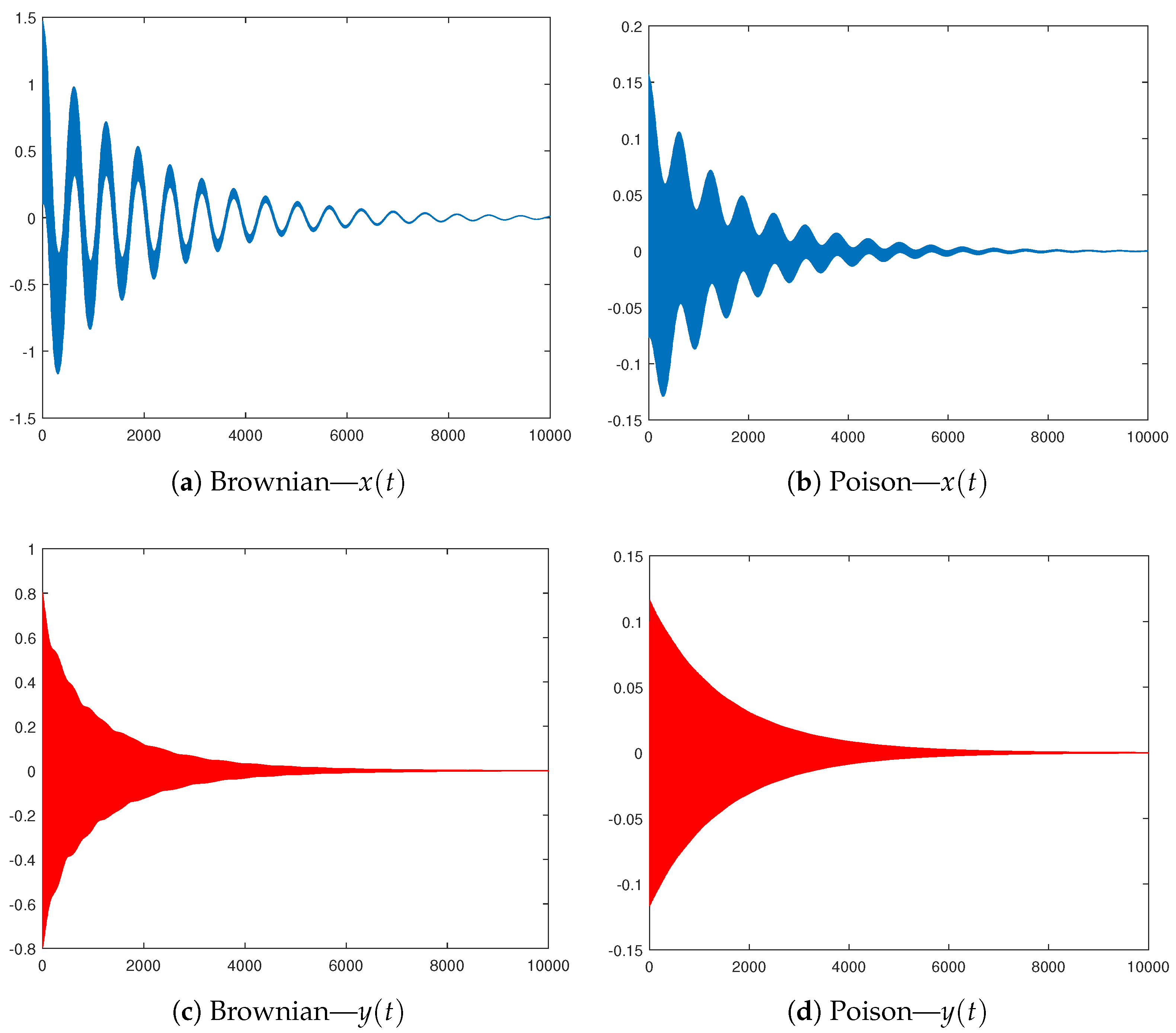
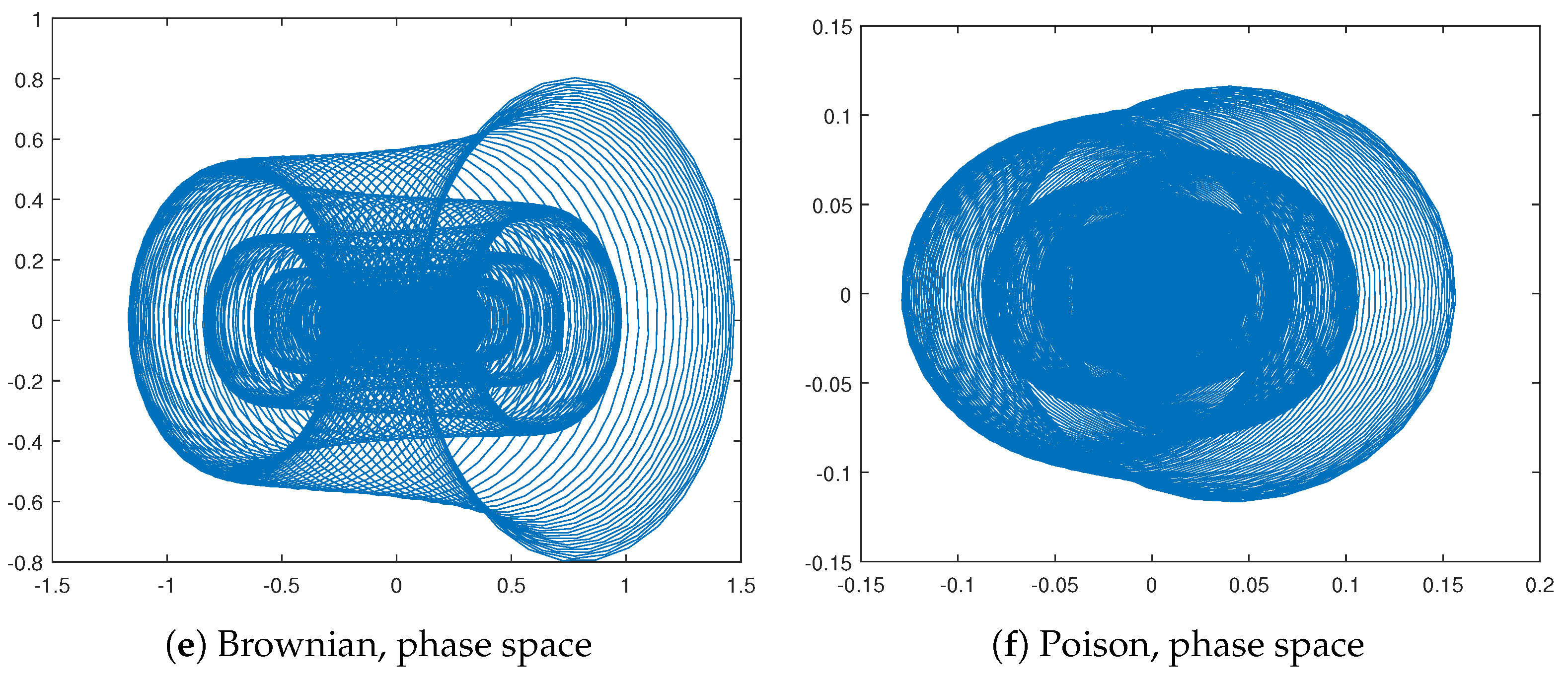
Appendix A. Stochastic Control on the Perturbations in Model A

Next, we discuss a stochastic control on the introduced perturbations. We first rewrite model (5) as follows
d x d t = y d y d t = sin x ϵ A y 1 | y | n 1 | y | j = 1 N g j sin ( j ω t ) .
We can assume without any restrictions that j = 1 N g j = 1 and, consequently, we can consider these coefficients to be the probabilities of a particular distribution. We shall follow the approach of [26,27,28]—we will briefly describe it. Using the complex presentation of the sin-function
sin x = e i x e i x 2 i ,
we can rewrite the y-dynamics (A1) as
d y d t = sin x ϵ A y 1 | y | n 1 | y | j = 1 N g j e i j ω t e i j ω t 2 i = sin x ϵ A y 1 | y | n 1 | y | 1 2 i ψ ω t ψ ω t .
Above, by ψ · is denoted the characteristic function of a distribution taking values 1 , 2 , , N with probabilities g j , j = 1 , 2 , , N . Note that we can generalize dynamics (A3) on the infinite support 1 , 2 , as well as on some continuous domain. Thus, if we denote the domain of the probability distribution by D and its density by g · , then the original dynamics (A1) turns into
d x d t = y d y d t = sin x ϵ A y 1 | y | n 1 | y | D g u sin ( u ω t ) d u .
In contrast to the approach used in [26,27,28], we shift the time dependence from the sin-function to the function g · , t , imposing the condition D g u , t d u = 1 for every fixed t. Thus, we view g · , t as the density function of a stochastic process. Thus, dynamics (A3) turn into
d y d t = sin x ϵ A y 1 | y | n 1 | y | 1 2 i ψ t , ω ψ t , ω .
Our suggestion is to use the characteristic function of a Brownian motion with drift μ and multiplied by a diffusion coefficient σ —its domain is D R . Its characteristic function is
ψ t , x = e t i μ x σ 2 x 2 2 .
Hence, dynamics (A5) can be written as
d y d t = sin x ϵ A y 1 | y | n 1 | y | 1 2 i e t i μ ω σ 2 ω 2 2 e t i μ ω σ 2 ω 2 2 = sin x ϵ A y 1 | y | n 1 | y | e σ 2 ω 2 t 2 2 i e i μ ω t e i μ ω t = sin x ϵ A y 1 | y | n 1 | y | e σ 2 ω 2 t 2 sin μ ω t .
We present in Figure A1a,c,e the x- and y-dynamics as well as the phase portrait for the following values: p = 10 , A = 0.0012 , ϵ = 1 , ω = 0.1 , μ = 0.1 , and σ = 0.3 . The initial point is assumed to be 0.1 , 0.1 .
Suppose now that the perturbations are driven by the characteristic function of a Poisson point process with intensity λ , i.e.,
ψ t , x = e λ t e i x 1 .
Using formula (A2), we rewrite
1 2 i ψ t , ω ψ t , ω = 1 2 i e λ t e i ω 1 e λ t e i ω 1 = e λ t 2 i e λ t cos ω + i sin ω e λ t cos ω i sin ω = e λ t 2 i e λ t cos ω e i λ t sin ω e i λ t sin ω = e λ t cos ω 1 sin λ t sin ω .
Hence, y-dynamics (A7) turns into
d y d t = sin x ϵ A y 1 | y | n 1 | y | e λ t cos ω 1 sin λ t sin ω .
Some simulations based on this construction can be seen in Figure A1b,d,f. We use the values p = 10 , A = 0.03 , ϵ = 0.04 and λ = 0.1 .
Figure A1. Oscillators based on the Brownian motion and the Poisson process.
Mathematics 13 00231 g0a1

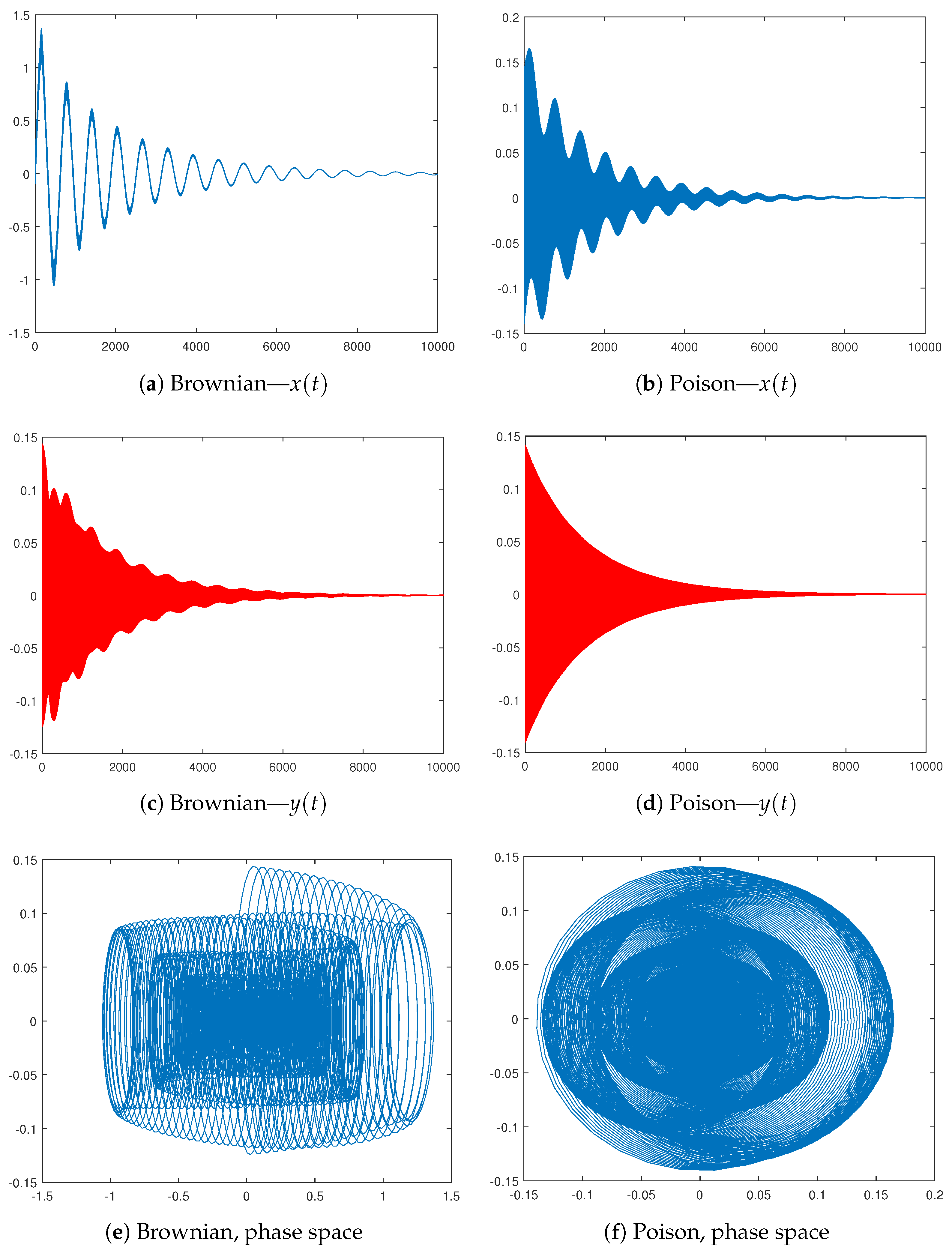
Appendix B. Stochastic Control on the Perturbations in Model B

We discuss briefly Model B in light of the approach presented in the previous section. Using the cos-presentation
cos x = e i x + e i x 2 ,
we transform dynamics (15) into
d x d t = y d y d t = sin x ϵ A y 1 | y | n 1 | y | + cos x 2 ψ t , ω + ψ t , ω .
If we use the Brownian characteristic function (A6), we reach
d y d t = sin x ϵ A y 1 | y | n 1 | y | + cos x e σ 2 ω 2 t 2 cos μ ω t .
If we apply the Poisson characteristic function (A8), then dynamics (A13) turns into
d y d t = sin x ϵ A y 1 | y | n 1 | y | + cos x e λ t cos ω 1 cos λ t sin ω .
Some simulations based on the parameters reported in Appendix A are presented in Figure A2.
Figure A2. Oscillators based on the Brownian motion and the Poisson process.
Mathematics 13 00231 g0a2aMathematics 13 00231 g0a2b

References

  1. Tricomi, F. Integratione di un’ equazione differenziale presentatasi in elettrotecnica. Ann. Della Sc. Norm. Super. Pisa 1933, 2, 1–20. [Google Scholar]
  2. Stoker, J. Nonlinear Vibration in Mechanical and Electrical Systems; Interscience: New York, NY, USA, 1950. [Google Scholar]
  3. Levi, M.; Hoppensteadt, F.; Miranker, W. Dynamics of the Josephson junction. Q. Appl. Math. 1978, 35, 167–198. [Google Scholar] [CrossRef]
  4. Perko, L. Differential Equations and Dynamical Systems; Springer-Verlag: New York, NY, USA, 1991. [Google Scholar]
  5. Guckenheimer, J.; Holmes, P. Nonlinear Oscillations, Dynamical Systems, and Bifurcations of Vector Fields; Springer: New York, NY, USA, 1983. [Google Scholar]
  6. Sanjuan, M. The effect of nonlinear damping on the universal oscillator. Int. J. Bifurc. Chaos 1999, 9, 735–744. [Google Scholar] [CrossRef]
  7. Soliman, M.; Thompson, J. The effect of nonlinear damping on the steady state and basin bifurcation patterns of a nonlinear mechanical oscillator. Int. J. Bifurc. Chaos 1992, 2, 81–91. [Google Scholar] [CrossRef]
  8. Fangnon, R.; Ainamon, C.; Monwanou, A.; Mowadinou, C.; Orpu, J. Nonlinear dynamics of the quadratic damping Helmholtz oscillator. Complexity 2020, 2020, 8822534. [Google Scholar] [CrossRef]
  9. Bikdash, M.; Balachandran, B.; Nayfeh, A. Melnikov analysis for a ship with a general roll-damping model. Nonlinear Dyn. 1994, 6, 101–124. [Google Scholar] [CrossRef]
  10. Ravindra, B.; Mallik, A. Stability analysis of a non–linearly clamped Duffing oscillator. J. Sound Vib. 1999, 171, 708–716. [Google Scholar] [CrossRef]
  11. Ravindra, B.; Mallik, A. Role of nonlinear dissipation in soft Duffing oscillators. Phys. Rev. E 1984, 49, 4950–4954. [Google Scholar] [CrossRef] [PubMed]
  12. Sanjuan, M. Monoclinic bifurcation sets of driven nonlinear oscillators. Int. J. Theor. Phys. 1996, 35, 1745–1752. [Google Scholar] [CrossRef]
  13. Holmes, P.; Marsden, J. Horseshoes in perturbation of Hamiltonian systems with two degrees of freedom. Commun. Math. Phys. 1982, 82, 523–544. [Google Scholar] [CrossRef]
  14. Holmes, P.; Marsden, J. A partial differential equation with infinitely many periodic orbits: Chaotic oscillations. Arch. Ration. Mech. Anal. 1981, 76, 135–166. [Google Scholar] [CrossRef]
  15. Golev, A.; Terzieva, T.; Iliev, A.; Rahnev, A.; Kyurkchiev, N. Simulation on a Generalized Oscillator Model: Web-Based Application. Proc. Bulg. Acad. Sci. 2024, 77, 230–237. [Google Scholar] [CrossRef]
  16. Lenci, S.; Lupini, R. Homoclinic and heteroclinic solutions for a class of two-dimensional Hamiltonian systems. Z. Angew. Math. Phys. 1996, 47, 97–111. [Google Scholar] [CrossRef]
  17. Lenci, S.; Rega, G. Controlling nonlinear dynamics in a two-well impact system. I. Attractors and bifurcation scenario under symmetric excitations. Int. J. Bifur. Chaos Appl. Sci. Eng. 1998, 8, 2387–2407. [Google Scholar] [CrossRef]
  18. Lenci, S.; Rega, G. Controlling nonlinear dynamics in a two-well impact system. II. Attractors and bifurcation scenario under unsymmetric optimal excitation. Int. J. Bifur. Chaos Appl. Sci. Eng. 1998, 8, 2409–2424. [Google Scholar] [CrossRef]
  19. Lenci, S.; Rega, G. Higher-order Melnikov analysis of homo/heteroclinic bifurcations in mechanical oscillators. In Proceedings of the 16th AIMETA Congress of Theoretical and Applied Mechanics, Ferrara, Italy, 9–12 September 2003. CD-Rom. [Google Scholar]
  20. Lenci, S.; Rega, G. Optimal control of homoclinic bifurcation: Theoretical treatment and practical reduction of safe basin erosion in the Helmholtz oscillator. J. Vib. Control 2003, 9, 281–315. [Google Scholar] [CrossRef]
  21. Rega, G.; Lenci, S. Bifurcations and chaos in single-d.o.f. mechanical systems: Exploiting nonlinear dynamics properties for their control. In Recent Research Developments in Structural Dynamics; Luongo, A., Ed.; Research Signpost: Kerala, India, 2003; pp. 331–369. [Google Scholar]
  22. Melnikov, V. On the stability of a center for time–periodic perturbation. Trans. Mosc. Math. Soc. 1963, 12, 3–52. [Google Scholar]
  23. Kyurkchiev, N.; Zaevski, T.; Iliev, A.; Kyurkchiev, V.; Rahnev, A. Nonlinear dynamics of a new class of micro-electromechanical oscillators–open problems. Symmetry 2024, 16, 253. [Google Scholar] [CrossRef]
  24. Kyurkchiev, N.; Zaevski, T.; Iliev, A.; Kyurkchiev, V.; Rahnev, A. Dynamics of a new class of oscillators: Melnikov’s approach, possible application to antenna array theory. Math. Inform. 2024, 67, 367. [Google Scholar]
  25. Kyurkchiev, N.; Zaevski, T.; Iliev, A.; Kyurkchiev, V.; Rahnev, A. Modeling of Some Classes of Extended Oscillators: Simulations, Algorithms, Generating Chaos, Open Problems. Algorithms 2024, 17, 121. [Google Scholar] [CrossRef]
  26. Kyurkchiev, N.; Zaevski, T.; Iliev, A.; Branzov, T.; Kyurkchiev, V.; Rahnev, A. Dynamics of Some Perturbed Morse-Type Oscillators: Simulations and Applications. Mathematics 2024, 12, 3368. [Google Scholar] [CrossRef]
  27. Kyurkchiev, N.; Zaevski, T.; Iliev, A.; Kyurkchiev, V.; Rahnev, A. Notes on Modified Planar Kelvin–Stuart Models: Simulations, Applications, Probabilistic Control on the Perturbations. Axioms 2024, 13, 720. [Google Scholar] [CrossRef]
  28. Kyurkchiev, N.; Zaevski, T.; Iliev, A.; Kyurkchiev, V.; Rahnev, A. Generating Chaos in Dynamical Systems: Applications, Symmetry Results, and Stimulating Examples. Symmetry 2024, 16, 938. [Google Scholar] [CrossRef]
  29. Proinov, P.; Vasileva, M. On the convergence of high-order Gargantini-Farmer-Loizou type iterative methods for simultaneous approximation of polynomial zeros. Appl. Math. Comput. 2019, 361, 202–214. [Google Scholar] [CrossRef]
  30. Ivanov, S. Families of high-order simultaneous methods with several corrections. Numer. Algorithms 2024, 97, 945–958. [Google Scholar] [CrossRef]
  31. Soltis, J. New Gegenbauer-like and Jacobi-like polynomials with applications. J. Frankl. Inst. 1993, 33, 635–639. [Google Scholar] [CrossRef]
  32. Chacon, R. Control of homoclinic chaos by weak periodic perturbations. In World Scientific Series on Nonlinear Science; Chua, L., Ed.; Series A; World Scientific Publisher: Singapore, 2005; Volume 55. [Google Scholar]
  33. Saghafi, A.; Furshidianfer, A. The analytical study of controlling chaotic dynamics in spur gear systems. Mech. Mach. Theory 2016, 96, 179–191. [Google Scholar] [CrossRef]
  34. Guerine, A. Dynamic response of a spur gear system with uncertain parameters. J. Theor. Appl. Mech. 2016, 54, 1039–1049. [Google Scholar] [CrossRef]
  35. Dalpiaz, G.; Rivola, A.; Rubini, R. Dynamic modeling of gear systems for condition monitoring and diagnostics. Congr. Tech. Diagn. 1996, 185–192. [Google Scholar]
  36. Guerine, A.; El Hami, A.; Fakhfakh, T.; Haddar, M. A polynomial chaos method to the analysis of the dynamic behavior of spur gear system. Struct. Eng. Mech. 2015, 53, 819–831. [Google Scholar] [CrossRef]
  37. Guerine, A.; El Hami, A.; Walha, L.; Fakhfakh, T.; Haddar, M. A perturbation approach for the dynamic analysis of one stage gear system with uncertain parameters. Mech. Mach. Theory 2015, 92, 113–126. [Google Scholar] [CrossRef]
  38. Jin, B.; Bian, Y.; Liu, X.; Gao, Z. Dynamic Modeling and Nonlinear Analysis of a Spur Gear System Considering a Nonuniformly Distributed Meshing Force. Appl. Sci. 2022, 12, 12270. [Google Scholar] [CrossRef]
  39. Ritala, R.; Salomaa, M. Odd and even subharmonics and chaos in RF SQUIDS. J. Phys. C Solid State Phys. 1983, 16, 477–484. [Google Scholar] [CrossRef]
  40. Ritala. R.; Salomaa, M. Chaotic dynamics of periodically driven rf superconducting quantum interference devices. Phys. Rev. B 1984, 29, 6143. [Google Scholar] [CrossRef]
  41. Fesser, K.; Bishop, A.; Kumar, P. Chaos in rf SQUID’s. Appl. Phys. Lett. 1983, 43, 123–124. [Google Scholar] [CrossRef]
  42. Schieve, W.; Bulsara, A.; Jacobs, E. Homoclinic chaos in the rf superconducting quantum-interference device. Phys. Rev. A 1988, 37, 3541. [Google Scholar] [CrossRef] [PubMed]
  43. Ling, F.; Bao, G. A numerical implementations of Melnikov’s method. Phys. Lett. A 1987, 122, 413. [Google Scholar] [CrossRef]
  44. Salam, F. The Mel’nikov Technique for Highly Dissipative Systems. SIAM J. Appl. Math. 1987, 47, 232–243. [Google Scholar] [CrossRef]
  45. Schecter, S. Melnikov’s method at a saddle–node and the dynamics of the forced Josephson junction. SIAM J. Math. Anal. 1987, 18, 1699–1715. [Google Scholar] [CrossRef]
  46. Grebogi, C.; Ott, E.; Yorke, J. Basin boundary metamorphoses: Changes in accessible boundary orbits. Physica 1987, 24, 243–262. [Google Scholar]
  47. Bruhn, B.; Koch, B. Homoclinic and Heteroclinic Bifurcations in rf SQUIDs. Z. Naturforschung 1988, 43, 930–938. [Google Scholar] [CrossRef]
  48. Ostrovskii, V.; Karimov, A.; Rybin, V.; Kopets, E.; Butusov, D. Comparing the Finite-Difference Schemes in the Simulation of Shunted Josephson Junctions. In Proceedings of the 23rd Conference of Open Innovations Association (FRUCT), Bologna, Italy, 13–16 November 2018; pp. 300–305. [Google Scholar]
Figure 1. The orbits ( x 0 ( t ) , y 0 ( t ) ) .
Mathematics 13 00231 g001
Figure 2. Using the formula M ( t 0 ) = 0 (Proposition 1).
Mathematics 13 00231 g002
Figure 3. Using the formula M ( t 0 ) = 0 (Proposition 2).
Mathematics 13 00231 g003
Figure 4. Using the formula M ( t 0 ) = 0 (Proposition 3).
Mathematics 13 00231 g004
Figure 5. Using the formula M ( t 0 ) = 0 (Proposition 4).
Mathematics 13 00231 g005
Figure 6. Using the formula M ( t 0 ) = 0 (Proposition 4).
Mathematics 13 00231 g006
Figure 7. Using the formula M ( t 0 ) = 0 (Proposition 5).
Mathematics 13 00231 g007
Figure 8. The system’s solutions (a); phase space (b) (example 1).
Mathematics 13 00231 g008
Figure 9. The system’s solutions (a); phase space (b) (example 2).
Mathematics 13 00231 g009
Figure 10. The system’s solutions (a); phase space (b) (example 3).
Mathematics 13 00231 g010
Figure 11. A typical Melnikov antenna array (from Proposition 4).
Mathematics 13 00231 g011
Figure 12. A typical Melnikov antenna array (from Proposition 6).
Mathematics 13 00231 g012
Figure 13. Using the formula M ( t 0 ) = 0 (Proposition 7).
Mathematics 13 00231 g013
Figure 14. Using the formula M ( t 0 ) = 0 (Proposition 8).
Mathematics 13 00231 g014
Figure 15. Using the formula M ( t 0 ) = 0 (Proposition 9).
Mathematics 13 00231 g015
Figure 16. Using the formula M ( t 0 ) = 0 (Proposition 9).
Mathematics 13 00231 g016
Figure 17. The system’s solutions (a); phase space (b) (example 1).
Mathematics 13 00231 g017
Figure 18. The system’s solutions (a); phase space (b) (example 2).
Mathematics 13 00231 g018
Figure 19. A typical Melnikov antenna array (from Proposition 8).
Mathematics 13 00231 g019
Figure 20. A typical Melnikov antenna array (from Proposition 9).
Mathematics 13 00231 g020
Figure 21. Using the formula M ( t 0 ) = 0 (Proposition 10).
Mathematics 13 00231 g021
Figure 22. Using the formula M ( t 0 ) = 0 (Proposition 10).
Mathematics 13 00231 g022
Figure 23. A typical Melnikov antenna array (from Proposition 10).
Mathematics 13 00231 g023
Figure 24. (a) The equation M ( t 0 ) = 0 (Proposition 11); (b) A typical array of Melnikov antennas (from Proposition 11).
Mathematics 13 00231 g024
Figure 25. Melnikov function M ( t 0 ) (Proposition 12).
Mathematics 13 00231 g025
Disclaimer/Publisher’s Note: The statements, opinions and data contained in all publications are solely those of the individual author(s) and contributor(s) and not of MDPI and/or the editor(s). MDPI and/or the editor(s) disclaim responsibility for any injury to people or property resulting from any ideas, methods, instructions or products referred to in the content.

