Abstract
American options have long received considerable attention in the literature, with numerous publications dedicated to their pricing. Bermudan and randomized Bermudan options are broadly used to estimate their prices efficiently. Notably, the penalty method yields option prices that coincide with those of randomized Bermudan options. However, theoretical results regarding the speed of convergence of these approximations to the American option price remain scarce. In this paper, we address this gap by establishing a general result on the convergence speed of Bermudan and randomized Bermudan option prices to their American limits. We prove that for convex payoff functions, the convergence speed is linear; that is, of order , where n denotes the number of exercisable opportunities in the Bermudan case and serves as the intensity parameter of the underlying Poisson process in the randomized Bermudan case. Our framework is quite general, encompassing Lévy models, stochastic volatility models, and nearly any risk-neutral model that can be incorporated within a strong Markov framework. We extend our analysis to Canadian options, showing under mild conditions a convergence rate of to their American limits. To our knowledge, this is the first study addressing the speed of convergence in Canadian option pricing.
MSC:
60G40; 91G20; 91G60
1. Introduction
Due to their importance and the challenges of pricing them, there has been a lot of interest in American options. Many numerical schemes use Bermudan options as proxies to estimate the price P of an American option. With linear extrapolation, the convergence may be accelerated. Extremely efficient examples are the CONV [1] and COS methods [2]. For Lévy models, they allow for the very rapid and accurate evaluation of Bermudan options. Let n denote the number of discrete exercise opportunities within the maturity period T, with intervals of length . It is assumed [1] (p. 1692) that an expansion of the Bermudan price in powers of exists with constant coefficients that is
with and not depending on n. When such an expansion exists, we say that smooth convergence occurs. Then, it is possible [3,4] to use repeated Richardson extrapolation (RRE) to obtain extremely fast convergence of the Bermudan price to its American limit. It is noted in [1] that is consistent with numerical experiments. However, to the best of our knowledge, the existence of an expansion in powers of has never been established, even in the Black–Scholes model. Outside the Black–Scholes setting, it has not yet even been proved that the convergence of Bermudan option prices to the American put is linear; that is, the speed of convergence is .
When an option can be exercised at maturity, or prior to maturity, at any of the jumps of an independent Poisson process N with intensity proportional to n, we have a randomized Bermudan option. The scheme has been studied under different names by many authors, such as in [5,6,7,8,9,10,11,12,13,14]. In the finite maturity case, it was shown in [7,11] (see also [9]) that the price of such options corresponds to the classical solution of the penalty method introduced in [15], which is widely acknowledged to be an efficient [16] way of pricing American options.
As far as we are aware, very few results have been established about the speed of convergence of Bermudan or randomized Bermudan option prices, in spite of the fact that both are broadly used in the computation of American options. In the Black–Scholes model with convex payoff functions, a speed of convergence of is obtained in [6,16,17], where n is the reciprocal of the (expected) time between two exercise opportunities. For Lévy models, a convergence speed of order is obtained in [7,16]. The speed of convergence depends on the convexity of the payoff function: indeed, it is shown in [16] that for non-convex payoff, the optimal speed of convergence can be of order . The most important case is the convex case since it includes the American put. We are not aware of any convergence speed results for stochastic volatility models. In the Volterra Heston model [18,19], which includes rough volatility models, convergence of Bermudan option prices is established in [20] for the put option and other non-smooth payoff functions. In [21], the authors study a form of modified Bermudan options through the lens of discrete approximations and corrected stopping boundaries, achieving a convergence rate of in the context of geometric Brownian motion.
The approximation of the American option price using Bermudan options or randomized Bermudan options (i.e., the penalty method) is broadly used in the literature. But how good is that approximation? What is the speed of convergence? Several articles, such as [22,23,24,25,26], refer to [17] or [1,2,3] to support the assumption that the convergence of Bermudan option prices to the American limit is linear or even smooth. However, in [1,2,3], linear and smooth convergence are mere assumptions backed by numerical experimentations. As pointed out in [1,2] it appears that [17] is the only paper in which an expansion of the Bermudan option price in terms of is considered and linear convergence is established; that is, the error decreases to zero at a speed of order , where is the expected time between two exercisable times.
Despite this sparse theoretical foundation, many papers, for instance [1,10,17,20,22,23,24,25,26,27,28,29,30,31,32,33,34,35], rely on the assumption of smooth or rapid convergence of the (randomized) Bermudan scheme to its American limit. This gap is the main motivation for this paper. We believe that establishing a general result of linear convergence of (randomized) Bermudan option prices to their American limit is long overdue. In a broad setting, we prove that (randomized) Bermudan option prices converge at a speed of for convex payoff functions. This is the main contribution of this article to the literature.
As an application of the results in this paper, we also show that under mild conditions, Canadian option prices converge at a speed of to their American limit, when the intensity of the associated Poisson process tends to infinity. To the best of our knowledge, it is the first time that the speed of convergence of Carr’s maturity-randomized option is studied, in spite of the immense popularity and influence of [36]. This is the second contribution of this article to the literature.
The paper is organized in the following manner. First, we gather the notation and assumptions used throughout this paper. Then, we establish the maximal expected gain that can result from an immediate exercise of the option rather than a randomly delayed one. Next, we prove the linear convergence of randomized Bermudan option prices to their American limits. As a corollary, we obtain the same speed of convergence for Bermudan options. Finally, we study the speed of convergence of Canadian options.
2. Setting, Notation and Assumptions
- Discounted underlying asset price. For simplicity, we assume a constant interest rate, . We also assume that the underlying asset is risk-neutral, meaning is a martingale. As is meant to be the price of some underlying asset, we also require that . Furthermore, we consider an associated process such that the pair forms a right process. A typical example arises in stochastic volatility models where represents the stochastic volatility, making a Markov process even though alone is not. If is already a right process, can be omitted. Recall that right processes form a very broad class of strong Markov processes characterized by càdlàg (right-continuous with left limits) trajectories. This class encompasses Hunt, Feller, Lévy, and diffusion processes, such as geometric Brownian motion, among others. As noted in [37], “the requirement of the strong Markov property is not onerous, as this includes solutions of stochastic differential equations and integrals of Lévy processes, so almost all common models used in quantitative finance”. The additional condition that the strong Markov process be a right process is similarly unrestrictive.
- Payoff functions. Recall that the value is called the intrinsic value of the option at time t. For simplicity, we consider payoff functions which are bounded, convex, and Lipschitz with compact support. For the American put, , for some .Probability space and counting process N. We consider a probability space, denoted by , which satisfies the usual conditions. We assume that the processes and a counting process are realized on this probability space, with being independent of .
- Conditional expectation notation. In this article, denotes the conditional expectation given that . Similarly, denotes the conditional expectation given that , and denotes the conditional expectation given that .
- Stopping time . Fix and an integer , we denote by the first time such that .
- Randomized options. Throughout this paper, we fix some maturity , a payoff function h, and some integer . In order to avoid undue generality, we focus on two cases: (a) the Poisson case, where is a Poisson process with intensity ; and (b) the deterministic case where the jumps of occur at times , for . We are interested in the following randomized American-style options, which at time can be described in the following manner:
- The Canadian option can be exercised at any time until .
- The randomized Bermudan option can be exercised at times , for .
- Randomized option prices. Fix , integer , and the payoff function h. Suppose that , , and . We denote by the value of the American option, by the value of the randomized Bermudan option, and by the value of the Canadian option. For , let be the class of stopping times such that for every , . Then
- Let be the class of stopping times such that for every , , for . Then and for ,
- Note that the price of a randomized Bermudan option might be less than its intrinsic value since, by definition, it is not exercisable at inception. An optimal stopping time exists: it is the first exercisable time at which the intrinsic value is no less than the option’s value. Note also that replacing by does not affect the value of the randomized Bermudan option because the increments of a Poisson process are independent and identically distributed. (In the deterministic case, where the jumps of occur at times , the value of is uniquely determined by t).Uniform -terms. Consider real valued functions , and , where for some arbitrary set . We say that uniformly if there exists a function such that for every and a constant c, that may depend only on and h, such that for every . In this paper, all O-terms are uniform.
3. Convergence Speed of Randomized Options
3.1. Maximal Immediate Expected Gain
Here, we establish a uniform upper bound in the form of an O-term for the expected gain, should such a gain exist, that results from an immediate exercise of the option rather than a randomly delayed one. The underlying context is the following: assume that is a point on the optimal exercise boundary of some American option in the setting of Section 2. Assume that m jumps of N have been observed. How bad is it to delay the exercise until the next exercisable time ? Put differently, how advantageous is it to exercise now? Here, the immediate expected gain is defined as the difference between the intrinsic value and the expected discounted delayed intrinsic value, provided this difference is positive. Otherwise, the gain is null.
In the theorem below, we provide a maximal gain, the maximal immediate expected gain, in the form of an -term, which can be viewed as an upper bound for this gain in terms of the expected length of .
Fix , an integer , and the payoff function h. Suppose that , , and . Fix an integer , and let
We are interested in the class of stopping times , which are either mere constants, such as , or take the form , where and are constants satisfying . We refer to this class of stopping times as the N-stopping times because they depend only on the process N and are completely independent of the trajectories of for .
Theorem 1
(Maximal immediate expected gain). Under the settings of Section 2, let , let , and let be an integer. Additionally, let θ be an N-stopping time such that , and define . Then
where the -term is uniform, and is the conditional expectation given that .
Proof.
Fix , , and an integer . Recall that is the conditional expectation given that , is the conditional expectation given that , and is the conditional expectation given that . Indeed, these quantities are the transition probability functions of their respective strong Markov right processes. Recall also that is independent of the process , for u restricted to the interval . Therefore, if is a non-negative bounded measurable function,
Note that
since depends in no way on the value of .
First, we show that
where the O-term is uniform. From the optional stopping theorem and the fact that is a martingale,
Then,
The reasoning yielding certainly holds if we replace by . Therefore,
This is equivalent to (2).
We will now establish (1). Utilizing the identity
and noting that for every
it follows, by the boundedness of h, that
Since h is Lipschitz with compact support, then for every ,
Using (2), we obtain
Thus,
Using Jensen’s inequality and (3), we get
The combination of this inequality and (4) yields
From the above inequality, we conclude that, if
then
Otherwise, if
then obviously
In both cases
Note that, throughout the proof, the -terms are uniform. □
3.2. Bermudan and Randomized Bermudan Options
Here, we first show that randomized Bermudan option prices converge to their American limits at a speed of . We then derive the convergence speed of Bermudan option prices as a corollary.
Theorem 2
(Randomized Bermudan options). Under the settings of Section 2, we have
and
where the O-terms are uniform in and .
Proof.
Fix and . Let be the first exercisable time after t. In the Poisson case, where is an exponential random variable with average which is independent of the process , and . In the deterministic case, where is the truncation of x. In this case, .
We first prove (5). Invoking Theorem 1, there exists a constant c such that for every ,
Because the first exercisable time after t is suboptimal:
Thus,
We now turn our attention to (6). But first, we introduce some notation. Let be the optimal stopping time for the American option, and let be the first exercisable time which is greater than or equal to . Let be the waiting time until ; that is, . Finally, let denote the discounted expectation of the payoff at time , given that , . By suboptimality,
From the strong Markov property of we obtain
Next,
Exploiting (7) and more specifically
we get
Since , we have obtained
as wanted. □
We now set aside the Poisson process to focus exclusively on the deterministic case, where the jumps of occur at fixed times for Obviously, under this setting, the “randomized” Bermudan option is actually exercisable at “non-random” times. Then, by definition, the difference between a Bermudan option and a randomized Bermudan option is that, when purchased at time , , the Bermudan option is exercisable at time , while the randomized Bermudan option is exercisable only at time . Therefore,
where is the value of a Bermudan option.
The speed of convergence of the Bermudan option price, which is of order , is obtained as a simple corollary to Theorem 2.
Corollary 1
(Bermudan options). Under the settings of Section 2, we have that for , ,
where the O-term is uniform.
3.3. Canadian Options
Here, we use the maximal immediate expected gain to study the convergence speed of Canadian options to their American limit. We make the following assumption, which is verified, in particular, in the Black–Scholes model studied by Carr [36].
Assumption 1.
Let be the price at time 0 of a European option with maturity u when and . We assume that the mapping is continuously differentiable when and that for every ,
where
Theorem 3
(Canadian options). Under the settings of Section 2 and Assumption 1, we have
where the -term is uniform. Here,
denotes the price of the Canadian option at time 0, and is the optimal stopping time satisfying .
Proof.
We will use Theorem 1, which has a boundedness condition on the stopping times involved, more specifically that they are bounded by . Recall that given t, is the first time such that . Now, starting at time 0, the probability that is outside the interval goes to zero exponentially fast as , and since h is bounded, if we set , then clearly,
where
We will refer to the option exercisable until time as the ‘modified’ Canadian option. The first step of the proof is to show that for ,
where the -term is uniform. Fix and . Let be the optimal stopping time for the modified Canadian option. Then, using the strong Markov property of , we write
where and . Since is optimal, we can continue with
Then, we invoke Theorem 1 to get (10).
Now we return to the value of the modified Canadian option at time 0 and write
where
Set and . From (10) and the Markov property we get that, for some constant c that may depend only on and h,
Note that the last equality follows from the fact that , being the sum of n independent exponentially distributed random variables with mean , follows an Erlang distribution with shape parameter n and scale parameter . Consequently, , which leads to
Independence of and N and Assumption 1 give
where . Thus
Set and note that
Set and
Then, because ,
Now and therefore
We will now demonstrate, using similar reasoning, that
which yields and completes the proof. Because the proof is very similar to what has just been done, we will only highlight the main steps.
First we use Theorem 1 to show that
where the -term is uniform. Next, if is the optimal stopping time for the American option at time 0, we write
Then, with (11) and the strong Markov property, we continue with
Setting , we conclude that
From this, we get
as wanted. □
4. Numerical Illustration
A closed-form formula for the value of a Bermudan put option in the Black–Scholes model is provided in [38]. However, as noted in [27], evaluating high-dimensional multivariate normal cumulative distribution functions makes the formula computationally impractical, even for a small number of exercise opportunities. Here, we instead employ a tree method—specifically that of [39]—with 100,000 time steps and Richardson extrapolation to estimate the prices of American and Bermudan options. The convergence properties of tree methods are well understood [40,41,42,43,44], and the simplicity of the approach makes it easy for interested readers to replicate our results. To demonstrate that Bermudan options converge to their American limit at a speed of order of , where m is the number of equally spaced exercise opportunities after inception, we price American and Bermudan put options with parameters , , , , and . Let denote the American option price, and the Bermudan option price with m exercise opportunities after inception. We calculate for . The plot numerically illustrates that is bounded, which is equivalent to . The results appear in Figure 1.
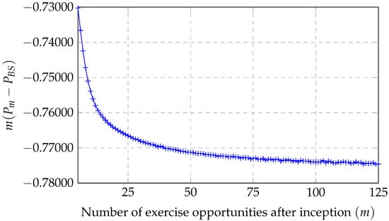
Figure 1.
The plot illustrates that remains bounded, which is equivalent to .
There is no closed-form formula for the value of Canadian options in the Black–Scholes setting. However, Carr [36] provides a numerical method to estimate their value. We use the same parameter values as above: , , , , and . Again, denotes the American put option price, but now denotes the price of a Canadian put option when the maturity occurs at the time of the mth jump of a Poisson process with intensity . We compute for . The plot numerically illustrates that is bounded, which is equivalent to . The results appear in Figure 2.
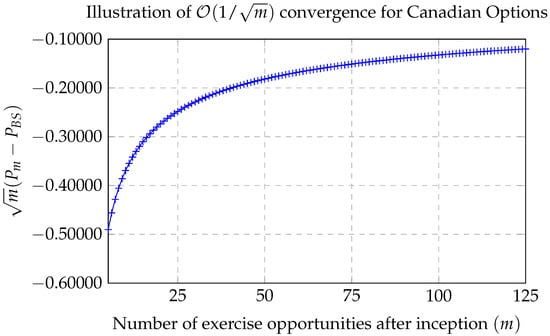
Figure 2.
The plot illustrates that remains bounded, which is equivalent to .
Funding
Guillaume Leduc was supported by the American University of Sharjah Faculty Research Grants FRG20-S-S83 and FRG24-E-S17. Furthermore, the work in this paper was also supported, in part, by the Open Access Program from the American University of Sharjah. This paper represents the opinions of the author and does not mean to represent the position or opinions of the American University of Sharjah.
Data Availability Statement
The original contributions presented in the study are included in the article, further inquiries can be directed to the author.
Conflicts of Interest
The author declares no conflicts of interest.
References
- Lord, R.; Fang, F.; Bervoets, F.; Oosterlee, C.W. A fast and accurate FFT-based method for pricing early-exercise options under Lévy processes. SIAM J. Sci. Comput. 2008, 30, 1678–1705. [Google Scholar] [CrossRef]
- Fang, F.; Oosterlee, C.W. Pricing early-exercise and discrete barrier options by Fourier-cosine series expansions. Numer. Math. 2009, 114, 27–62. [Google Scholar] [CrossRef]
- Chang, C.-C.; Chung, S.-L.; Stapleton, R.C. Richardson extrapolation techniques for the pricing of American-style options. J. Futur. Mark. 2007, 27, 791–817. [Google Scholar] [CrossRef]
- Chang, C.-C.; Lin, J.-B.; Tsai, W.-C.; Wang, Y.-H. Using Richardson extrapolation techniques to price American options with alternative stochastic processes. Rev. Quant. Financ. Account. 2012, 39, 383–406. [Google Scholar] [CrossRef]
- Dupuis, P.; Wang, H. Optimal stopping with random intervention times. Adv. Appl. Probab. 2002, 34, 141–157. [Google Scholar] [CrossRef]
- Dupuis, P.; Wang, H. On the convergence from discrete to continuous time in an optimal stopping problem. Ann. Appl. Probab. 2005, 15, 1339–1366. [Google Scholar] [CrossRef][Green Version]
- Eriksson, B.; Pistorius, M. American option valuation under continuous-time Markov chains. Adv. Appl. Probab. 2015, 47, 378–401. [Google Scholar] [CrossRef]
- Guo, X.; Liu, J. Stopping at the maximum of geometric Brownian motion when signals are received. J. Appl. Probab. 2005, 826–838. [Google Scholar] [CrossRef]
- Lange, R.-J.; Ralph, D.; Støre, K. Real-option valuation in multiple dimensions using Poisson optional stopping times. J. Financ. Quant. Anal. 2020, 55, 653–677. [Google Scholar] [CrossRef]
- Leduc, G. Exercisability randomization of the American option. Stoch. Anal. Appl. 2008, 26, 832–855. [Google Scholar] [CrossRef]
- Leduc, G. The randomized American option as a classical solution to the penalized problem. J. Funct. Spaces 2015, 2015, 245436. [Google Scholar] [CrossRef]
- Lempa, J. Optimal stopping with information constraint. Appl. Math. Optim. 2012, 66, 147–173. [Google Scholar] [CrossRef]
- Miclo, L.; Villeneuve, S. On the forward algorithm for stopping problems on continuous-time Markov chains. J. Appl. Probab. 2021, 58, 1043–1063. [Google Scholar] [CrossRef]
- Bayer, C.; Belomestny, D.; Hager, P.; Pigato, P.; Schoenmakers, J. Randomized optimal stopping algorithms and their convergence analysis. SIAM J. Financ. Math. 2021, 12, 1201–1225. [Google Scholar] [CrossRef]
- Forsyth, P.; Vetzal, K. Quadratic convergence for valuing American options using a penalty method. SIAM J. Sci. Comput. 2002, 23, 2095–2122. [Google Scholar] [CrossRef]
- Howison, S.; Reisinger, C.; Witte, J. The effect of nonsmooth payoffs on the penalty approximation of American options. SIAM J. Financ. Math. 2013, 4, 539–574. [Google Scholar] [CrossRef]
- Howison, S. A matched asymptotic expansions approach to continuity corrections for discretely sampled options. Part 2: Bermudan options. Appl. Math. Financ. 2007, 14, 91–104. [Google Scholar] [CrossRef]
- Abi Jaber, E.; El Euch, O. Markovian structure of the Volterra Heston model. Stat. Probab. Lett. 2019, 149, 63–72. [Google Scholar] [CrossRef]
- Abi Jaber, E.; Larsson, M.; Pulido, S. Affine Volterra processes. Ann. Appl. Probab. 2019, 29, 3155–3200. [Google Scholar] [CrossRef]
- Chevalier, E.; Pulido, S.; Zúñiga, E. American options in the Volterra Heston model. SIAM J. Financ. Math. 2022, 13, 426–458. [Google Scholar] [CrossRef]
- Lai, T.L.; Yao, Y.-C.; AitSahlia, F. Corrected random walk approximations to free boundary problems in optimal stopping. Adv. Appl. Probab. 2007, 39, 753–775. [Google Scholar] [CrossRef]
- Ballestra, L.V.; Cecere, L. A fast numerical method to price American options under the Bates model. Comput. Math. Appl. 2016, 72, 1305–1319. [Google Scholar] [CrossRef]
- Dilloo, M.J.; Tangman, D.Y. A high-order finite difference method for option valuation. Comput. Math. Appl. 2017, 74, 652–670. [Google Scholar] [CrossRef]
- Feng, L.; Lin, X. Pricing Bermudan options in Lévy process models. SIAM J. Financ. Math. 2013, 4, 474–493. [Google Scholar] [CrossRef]
- Gong, X.; Zhuang, X. American option valuation under time changed tempered stable Lévy processes. Phys. A Stat. Mech. Its Appl. 2017, 466, 57–68. [Google Scholar] [CrossRef]
- Shoude, H.; Guo, X. A Shannon wavelet method for pricing American options under two-factor stochastic volatilities and stochastic interest rate. Discret. Dyn. Nat. Soc. 2020, 2020, 8531959. [Google Scholar] [CrossRef]
- Bunch, D.S.; Johnson, H. A simple and numerically efficient valuation method for American puts using a modified Geske-Johnson approach. J. Financ. 1992, 47, 809–816. [Google Scholar]
- Chen, W.; Du, K.; Qiu, X. Analytic properties of American option prices under a modified Black–Scholes equation with spatial fractional derivatives. Phys. A Stat. Mech. Its Appl. 2018, 491, 37–44. [Google Scholar] [CrossRef]
- Huang, J.; Subrahmanyam, M.; Yu, G. Pricing and hedging American options: A recursive integration method. Rev. Financ. Stud. 1996, 9, 277–300. [Google Scholar] [CrossRef]
- Ibáñez, A. Robust pricing of the American put option: A note on Richardson extrapolation and the early exercise premium. Manag. Sci. 2003, 49, 1210–1228. [Google Scholar] [CrossRef]
- Jin, X.; Tan, H.H.; Sun, J. A state-space partitioning method for pricing high-dimensional American-style options. Math. Financ. 2007, 17, 399–426. [Google Scholar] [CrossRef]
- Lim, H.; Lee, S.; Kim, G. Efficient pricing of Bermudan options using recombining quadratures. J. Comput. Appl. Math. 2014, 271, 195–205. [Google Scholar] [CrossRef]
- Omberg, E. A note on the convergence of binomial-pricing and compound-option models. J. Financ. 1987, 42, 463–469. [Google Scholar]
- Prekopa, A.; Szántai, T. On the analytical–numerical valuation of the Bermudan and American options. Quant. Financ. 2010, 10, 59–74. [Google Scholar] [CrossRef]
- Shang, Q.; Byrne, B. American option pricing: Optimal lattice models and multidimensional efficiency tests. J. Futur. Mark. 2021, 41, 514–535. [Google Scholar] [CrossRef]
- Carr, P. Randomization and the American put. Rev. Financ. Stud. 1998, 11, 597. [Google Scholar] [CrossRef]
- Volk-Makarewicz, W.; Borovkova, S.; Heidergott, B. Assessing the impact of jumps in an option pricing model: A gradient estimation approach. Eur. J. Oper. Res. 2022, 298, 740–751. [Google Scholar] [CrossRef]
- Geske, R.; Johnson, H.E. The American put option valued analytically. J. Financ. 1984, 39, 1511–1524. [Google Scholar] [CrossRef]
- Chang, L.B.; Palmer, K. Smooth convergence in the binomial model. Financ. Stoch. 2007, 11, 91–105. [Google Scholar] [CrossRef]
- Joshi, M.S. The convergence of binomial trees for pricing the American put. J. Risk 2009, 11, 87–108. [Google Scholar] [CrossRef]
- Chan, J.H.; Joshi, M.; Tang, R.; Yang, C. Trinomial or binomial: Accelerating American put option price on trees. J. Futur. Mark. 2009, 29, 826–839. [Google Scholar] [CrossRef]
- Leduc, G.; Nurkanovic Hot, M. Joshi’s split tree for option pricing. Risks 2020, 8, 81. [Google Scholar] [CrossRef]
- Leduc, G. A European option general first-order error formula. ANZIAM J. 2013, 54, 248–272. [Google Scholar]
- Leduc, G.; Palmer, K. The convergence rate of option prices in trinomial trees. Risks 2023, 11, 52. [Google Scholar] [CrossRef]
Disclaimer/Publisher’s Note: The statements, opinions and data contained in all publications are solely those of the individual author(s) and contributor(s) and not of MDPI and/or the editor(s). MDPI and/or the editor(s) disclaim responsibility for any injury to people or property resulting from any ideas, methods, instructions or products referred to in the content. |
© 2025 by the author. Licensee MDPI, Basel, Switzerland. This article is an open access article distributed under the terms and conditions of the Creative Commons Attribution (CC BY) license (https://creativecommons.org/licenses/by/4.0/).