An Efficient GPU-Accelerated Algorithm for Solving Dynamic Response of Fluid-Saturated Porous Media

Abstract
1. Introduction
2. Theory and Methods
2.1. Wave Equation of Saturated Two-Phase Media in u-p Form
2.2. Explicit Time-Domain Solution
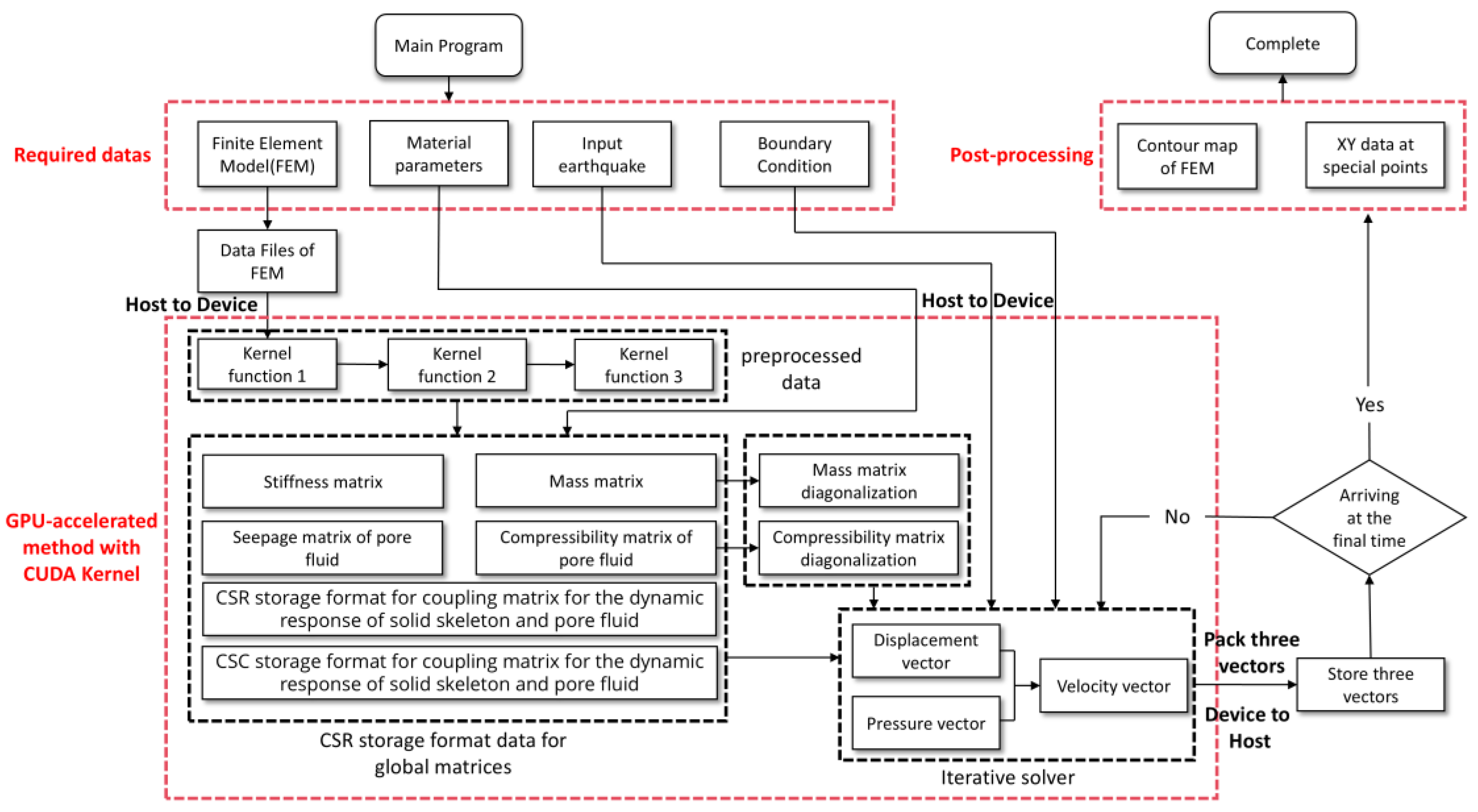
3. Implementation of the Kernel Function on a GPU
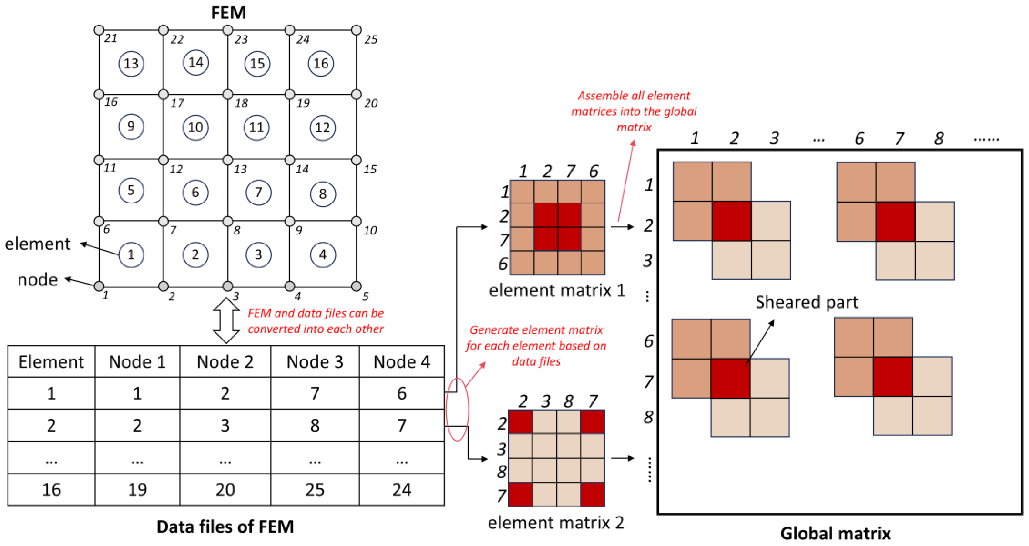
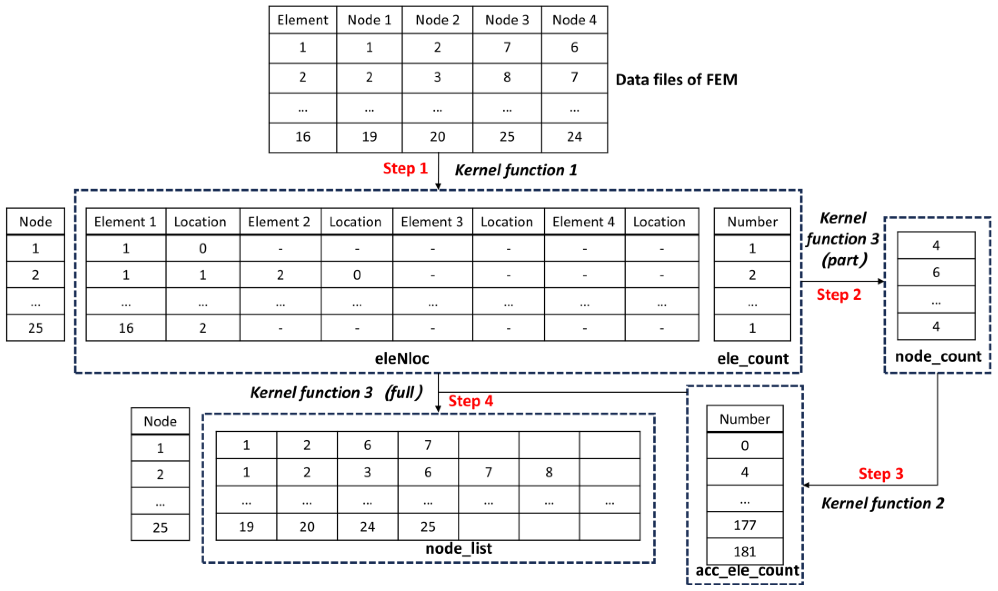
3.1. Resolve Thread Conflicts and Determine Relationships Between Nodes and Elements
| Algorithm 1: Use atomicAdd() to resolve thread conflicts and obtain the data of eleNloc and ele_count |
| 1: initial eleNloc to −1 and ele_count to 0 // The −1 is inserted to indicate that these numbers are not available. 2: MAX_ELEMENT←4 // MAX_ELEMENT represents the maximum number of elements shared by a node, which is set to 4. 3: x ← threadIdx.x + blockIdx.x * blockDim.x // x controls the serial number of the element ID. 4: for i = 0 to 3 do 5: node ← element(i) // element is the data files of FEM, and i shows 4 nodes. 6: temp_count ← atomicAdd(&ele_count[node],1) // This step resolves thread conflicts. 7: eleNloc[2 * (node-1) * MAX_ELEMENT + 2 * temp_count] ← x + 1 // element numbers start at 1, so +1 8: eleNloc[2 * (node-1) * MAX_ELEMENT + 2 * temp_count + 1] ← i // i is the location of node in the element, counting from 0 9: end for |
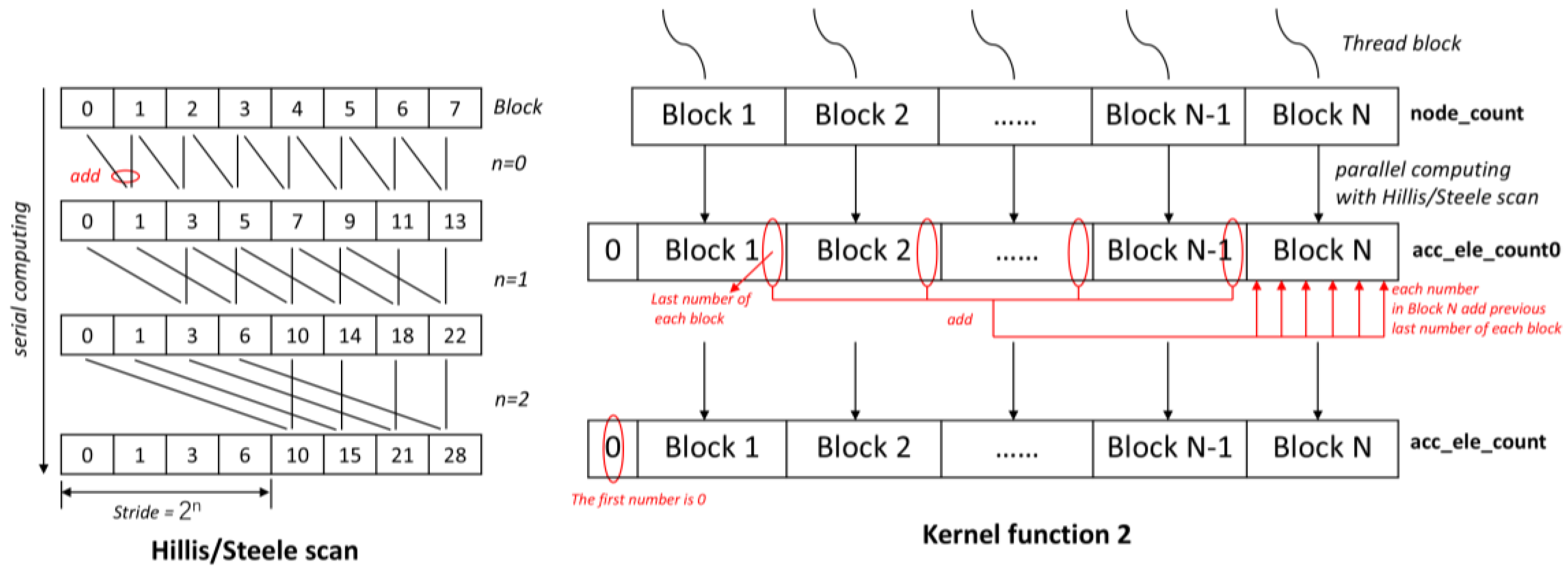
3.2. Obtaining the Data of the Prefix Sum
| Algorithm 2: From node_count to acc_ele_count0 |
| 1: buffer_idx ← threadIdx.x + blockDim.x * blockIdx.x // buffer_idx controls the serial number of the node. 2: BLOCK_SIZE←32 // BLOCK_SIZE is the size of kernel block and should not larger than 32, otherwise the data will be wrong. 3: __shared__ int cache[BLOCK_SIZE] 4: if buffer_idx< BLOCK_SIZE then // The first data is 0, and the other data is moved one position later. 5: cache[0] ← 0 6: cache[threadIdx.x+1] ← node_count[buffer_idx] 7: else 8: cache[threadIdx.x] ← node_count[buffer_idx-1] 9: end if 10: __syncthreads(); 11: for (int stride = 1; stride < blockDim.x; stride * = 2) { 12: if (threadIdx.x >= stride) { 13: cache[threadIdx.x] += cache[threadIdx.x − stride];} 14: __syncthreads();} 15: acc_ele_count0[buffer_idx] ← cache[threadIdx.x] |
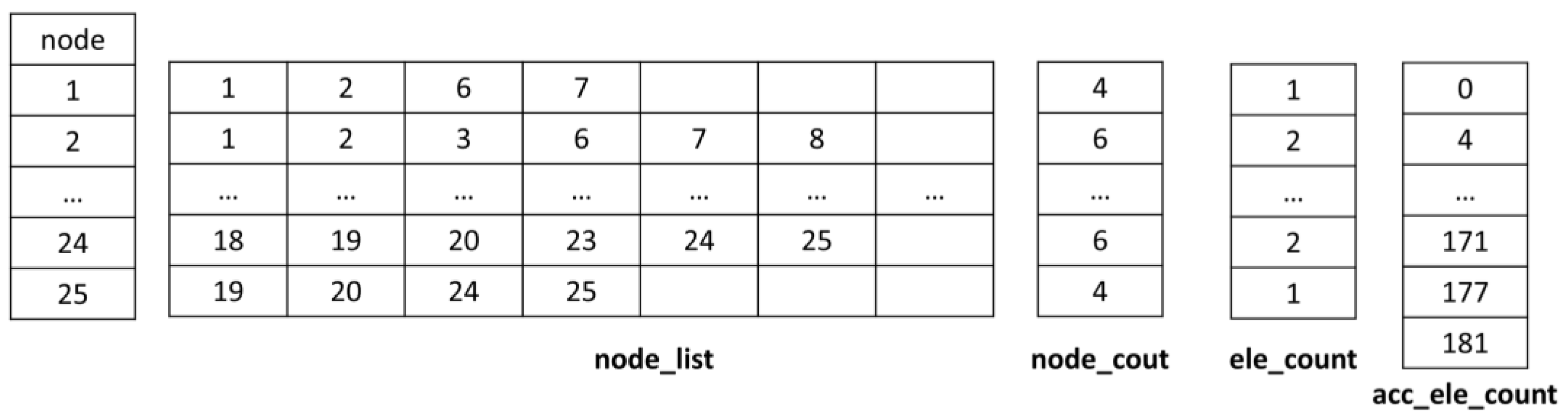
3.3. Obtaining the Relationship Between Nodes
| Algorithm 3: Obtain information about each node and its associated nodes (including itself) |
| 1: initial node_list to 0 2: x←threadIdx.x + blockIdx.x * blockDim.x // x controls the serial number of the node 3: element_num←4 * ele_count[x] // The number of nodes associated with a node can never exceed 4 * ele_count[x] 5: temp_node_list[element_num] ← −1 // Initialize the array temp_node_list to any number less than 0 (this is to make it easier to compare value of nodes with values of temp_node_list and sort them). 6: for element in eleNloc(x) do // Get all the elements of this node from eleNloc. 7: Get the nodes in element, sort them, and place them in the array temp_node_list. 8: end for 9: The value of node_count(x) is the amount in temp_node_list that is not −1. 10: element_num←node_count(x) 11: for i = 0 to element_num do 12: node_list[i + acc_ele_count[x]] ← temp_node_list[i] // Store the data from temp_node_list into node_list 13: end for |
3.4. Generate CSR and CSC Storage Format Data for Each Global Matrix
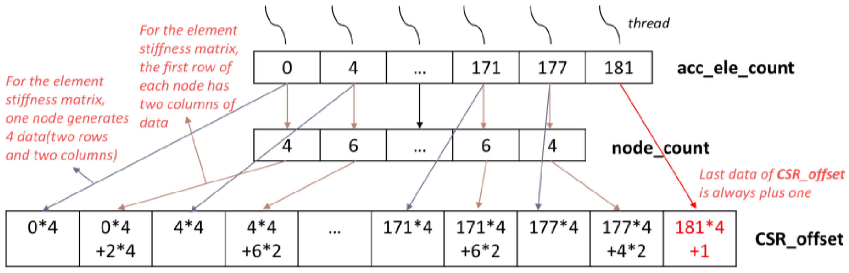
3.4.1. Generation of CSR_offset Data
| Algorithm 4: Generation of CSR_offset data for global stiffness matrix |
| 1: initial CSR_offset to 0 2: x ← threadIdx.x + blockIdx.x * blockDim.x // x controls the serial number of the node 3: element_num←node_count(x) 4: CSR_offset[2 * x] ← acc_ele_count[x] * 2 * 2 5: CSR_offset[2 * x + 1] ← acc_ele_count[x] * 2 * 2 + 2 * temp_count 6: if x = COORDS_NUM then // COORDS_NUM is the total number of nodes, and it’s 25 in this case 7: CSR_offset[2 * x] = acc_ele_count[x] * 2 * 2 + 1 // The last value of CSR_offset adds one 8: end if |
3.4.2. Generation of CSR_y Data
| Algorithm 5: Generation of CSR_y data for global stiffness matrix |
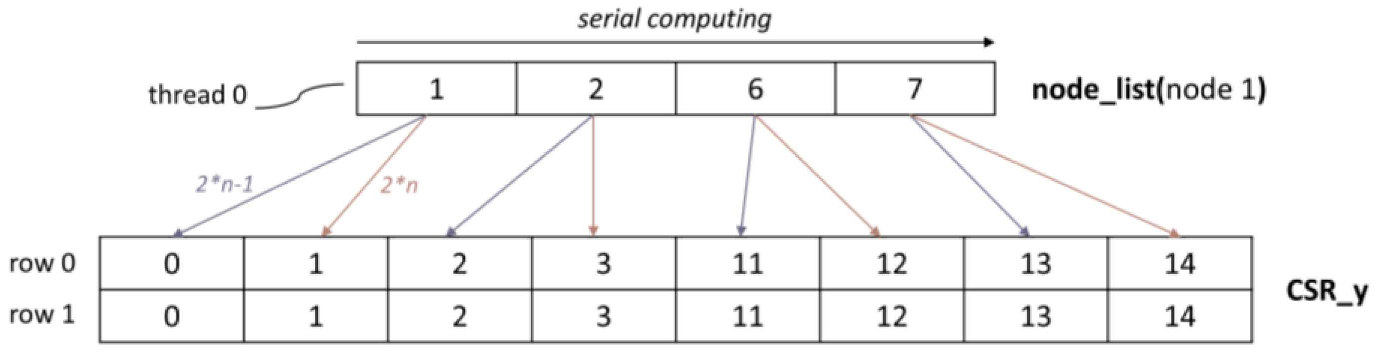
| 1: initial CSR_offset to 0 2: x ← threadIdx.x + blockIdx.x * blockDim.x / x controls the serial number of the node 3: element_num←node_count(x) 4: acc_ele_num ← acc_ele_count[x] 5: for i = 0 to temp_count do 6: CSR_y[2 * i + CSR_offset[2 * x]] ← 2 * node_list[acc_element_num + i] − 2 // The first element in the first row for a node. 7: CSR_y[2 * i + 1 + CSR_offset[2 * x]] ← 2 * node_list[acc_element_num + i] − 1 // The second element in the first row for a node. 8: CSR_y[2 * i + CSR_offset[2 * x + 1]] ← 2 * node_list[acc_element_num + i] − 2 // The first element in the second row for a node. 9: CSR_y[2 * i + 1 + CSR_offset[2 * x + 1]] ← 2 * node_list[acc_element_num + i] − 1 // The second element in the second row for a node. 10: end for |
3.4.3. Generation of CSR_value Data
| Algorithm 6: Generation of CSR_value data for global stiffness matrix |
| 1: initial CSR_value to 0 2: x ← threadIdx.x + blockIdx.x * blockDim.x / x controls the serial number of the node 3: element_num←node_count(x) 4: for K = 0 to ele_count[x] do // K controls element and location 5: element_N←eleNloc(K,x) // Gets the number of elment from eleNloc and assigns it to element_N. 6: element_loc←eleNloc(K,x) // Gets the elment location assignment from eleNloc to element_loc 7: Get the four nodes of each element, i,j,m,n, from data files of FEM 8: calculate ke(i,j,m,n) 10: for K = 0 to 4 do // Control four nodes. 11: if element_loc = K do // Control the position of nodes in the elements. 12: for M = 0 to element_num do // here is to compare the position of node_list with i,j,m,n. 13: Compare i,j,m,n with node_list(M,x) respectively, and then fill the data into the corresponding location. //The x in node_list(M,x) is to locate the data in node_list, for instance, node_list(node 2) in Figure 8. //for example, //if i = node_list(M,x) do CSR_value[2 * M + CSR_offset[2 * x]] += ke [2 * K][0]; CSR_value[2 * M + 1 + CSR_offset[2 * x]] += ke [2 * K][1]; CSR_value[2 * M + CSR_offset[2 * x + 1]] += ke [2 * K + 1][0]; CSR_value[2 * M + 1 + CSR_offset[2 * x + 1]] += ke [2 * K + 1][1]; end if 14: end for 15: end if 16: end for |
3.5. Description of Iterative Solution
| Algorithm 7: CUDA built-in spmv_csr function |
| 1: __global__ void spmv_csr(const int * row_ptr, const int * col_ind, const double * values, const int * num_rows, const double * x, double * y) { 2: // Uses a grid-stride loop to perform dot product 3: for (int i = blockIdx.x * blockDim.x + threadIdx.x; i < num_rows; i += blockDim.x * gridDim.x) { 4: ACCURACY dotProduct = 0; 5: const int row_start = row_ptr[i]; 6: const int row_end = row_ptr[i + 1]; 7: for (int j = row_start; j < row_end; j++) { 8: dotProduct += values[j] * x[col_ind[j]]; 9: } 10: y[i] = dotProduct; 11: } 12: } |
| Algorithm 8: Calculate uk+1 |
| 1: Kuk←K * Uk; // Using spmv_csr to calculate K * Uk, Kuk is the value of a row 2: Qpk←Q * pk; // Using spmv_csr to calculate Q * Pk, Qpk is the value of a row 3: for (int i = blockIdx.x * blockDim.x + threadIdx.x; i < TOTAL_COORDS_NUM * 2; i += blockDim.x * gridDim.x) { // TOTAL_COORDS_NUM is the number of all nodes. 4: uk+1[i]←uk[i] + Δt * k[i] + 0.5 * Δt2 * Ml−1[i] * (fuk[i] − Kuk + Qpk);} // Get the result |
4. Results and Analysis
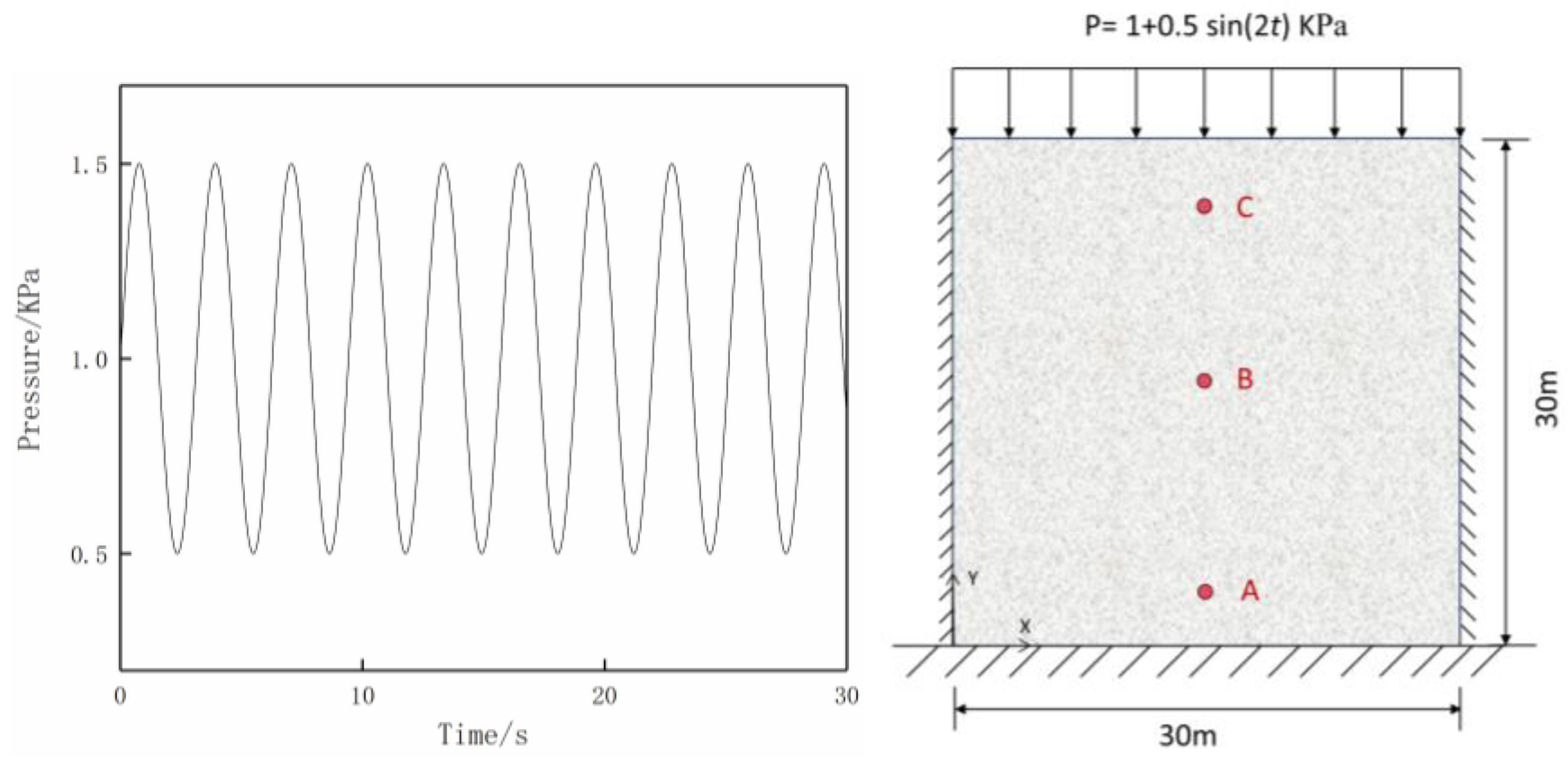
4.1. Example Simulation
4.2. Influence of Accuracy on Calculation Efficiency
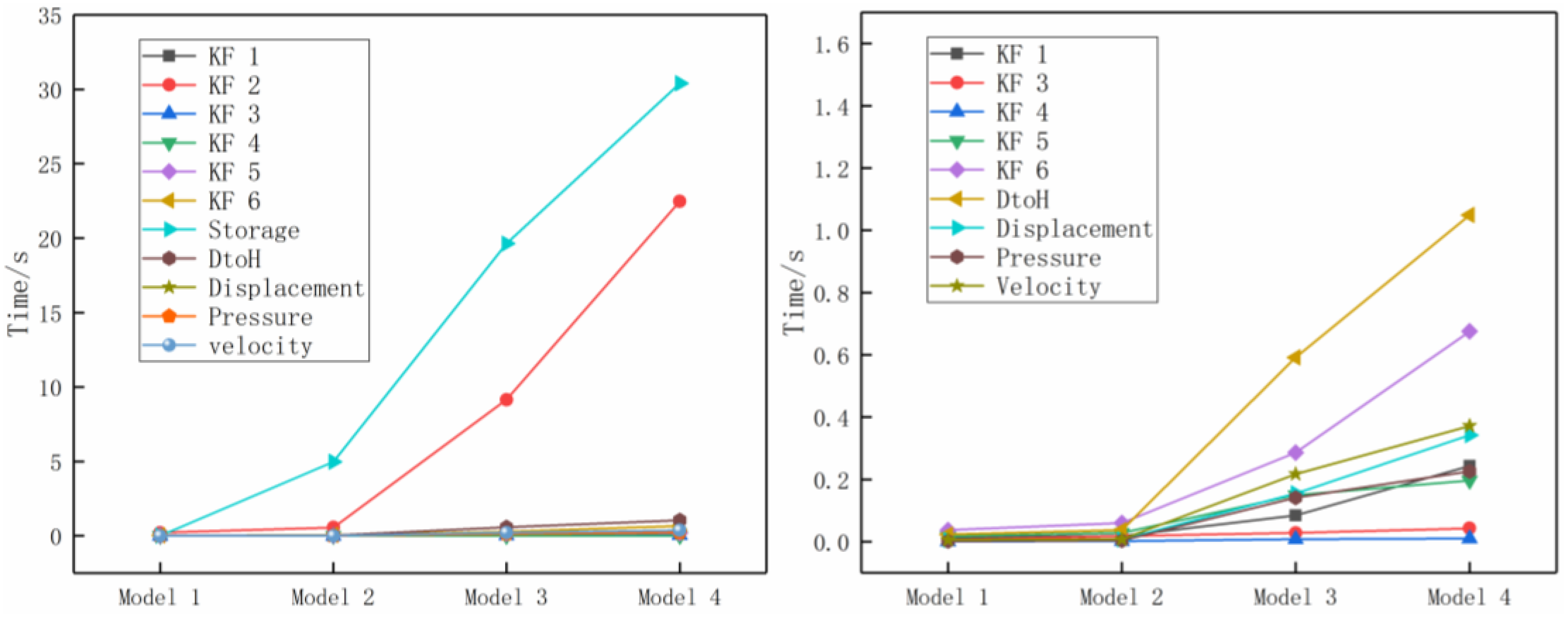
4.3. Influence of Model Size on Computing Efficiency
4.4. The Speedup Ratio of a GPU Program to a CPU Program
5. Conclusions
Author Contributions
Funding
Data Availability Statement
Conflicts of Interest
References
- Georgescu, S.; Chow, P.; Okuda, H. GPU acceleration for fem-based structural analysis. Arch. Comput. Methods Eng. 2013, 20, 111–121. [Google Scholar] [CrossRef] [Scilit]
- Fu, Z.; Lewis, T.J.; Kirby, R.M.; Whitaker, R.T. Architecting the finite element method pipeline for the GPU. J. Comput. Appl. Math. 2014, 257, 195–211. [Google Scholar] [CrossRef] [Scilit] [PubMed]
- Garland, M.; Kirk, D.B. Understanding throughput-oriented architectures. Commun. ACM 2010, 53, 58–66. [Google Scholar] [CrossRef] [Scilit]
- Zhu, Z.; Yang, X.; Li, H.; Xu, H.K.; Zhou, Y. A multi-GPU parallel computing method for 3D random vibration of train-track-soil dynamic interaction. J. Cent. South Univ. 2023, 30, 1722–1736. [Google Scholar] [CrossRef] [Scilit]
- Obrecht, C.; Kuznik, F.; Tourancheau, B.; Roux, J.J. Multi-gpu implementation of the lattice boltzmann method. Comput. Math. Appl. 2013, 65, 252–261. [Google Scholar] [CrossRef] [Scilit]
- Yuan, W.; Feng, X.S.; Zhou, Y.F.; Gan, X.B. A multi-GPU finite volume solver for magnetohydrodynamics-based solar wind simulations. Comput. Phys. Commun. 2019, 238, 181–193. [Google Scholar]
- Westphal, E.; Singh, S.P.; Huang, C.C.; Gompper, G.; Winkler, R.G. Multiparticle collision dynamics: GPU accelerated particle-based mesoscale hydrodynamic simulations. Comput. Phys. Commun. 2014, 185, 495–503. [Google Scholar] [CrossRef] [Scilit]
- Hassan, B.; Reza, M.; Ali, M.; Behnia, A.M.O. Pore size classification and prediction based on distribution of reservoir fluid volumes utilizing well logs and deep learning algorithm in a complex lithology. Artif. Intell. Geosci. 2024, 5, 100094. [Google Scholar]
- Behnia, A.M.O.; Reza, M.; Hassan, B.; Arzhan, M.H.; Abolfazl, K.M. Toward real-time fracture detection on image logs using deep convolutional neural network YOLOv5. Interpretation 2024, 2, 12. [Google Scholar]
- Pikle, N.K.; Sathe, S.R.; Vyavahare, A.Y. Low occupancy high performance elemental products in assembly free FEM on GPU. Eng. Comput. 2022, 38, 2189–2204. [Google Scholar] [CrossRef] [Scilit]
- Banas, K.; Plaszewski, P.; Maciol, P. Numerical integration on GPUs for higher order finite elements. Comput. Math. Appl. 2014, 67, 1319–1344. [Google Scholar] [CrossRef] [Scilit]
- Michéa, D.; Komatitsch, D. Accelerating a three-dimensional finite-difference wave propagation code using GPU graphics cards. Geophys. J. Int. 2010, 181, 389–402. [Google Scholar] [CrossRef] [Scilit]
- Dick, C.; Georgii, J.; Westermann, R. A real-time multigrid finite hexahedra method for elasticity simulation using CUDA. Simul. Model. Pract. Theory 2011, 19, 801–816. [Google Scholar] [CrossRef] [Scilit]
- Göddeke, D. Fast and Accurate Finite-Element Multigrid Solvers for PDE Simulations on GPU Clusters. Ph.D. Thesis, Fakultät für Mathematik, Technische Universität Dortmund, Dortmund, Germany, May 2010. [Google Scholar]
- Peter, H. Accelerated finite element elastodynamic simulations using the GPU. J. Comput. Phys. 2014, 257, 687–707. [Google Scholar]
- Komatitsch, D.; Michèa, D.; Erlebacher, G. Porting a high-order finite-element earthquake modeling application to NVIDIA graphics cards using CUDA. J. Parallel Distrib. 2009, 69, 451–460. [Google Scholar] [CrossRef] [Scilit]
- Cecka, C.; Lew, A.J.; Darve, E. Assembly of finite element methods on graphics processors. Int. J. Numer. Methods Eng. 2011, 85, 640–669. [Google Scholar] [CrossRef] [Scilit]
- Utpal, K.; Deepak, S.; Sachin, S.G. GPU-warp based finite element matrices generation and assembly using coloring method. J. Comput. Des. Eng. 2019, 4, 705–718. [Google Scholar]
- Woźniak, M. Fast GPU integration algorithm for isogeometric finite element method solvers using task dependency graphs. J. Comput. Sci. 2015, 11, 145–152. [Google Scholar] [CrossRef] [Scilit]
- Shewchuk, J.R. An Introduction to the Conjugate Gradient Method Without the Agonizing Pain; Carnegie Mellon University: Pittsburgh, PA, USA, 1994. [Google Scholar]
- Barrett, R.; Berry, M.W.; Chan, T.F.; Vorst, H.V.D. Templates for the Solution of Linear Systems: Building Blocks for Iterative Methods. Siam 1996, 43. [Google Scholar]
- Lin, S.; Xie, Z. A Jacobi_PCG solver for sparse linear systems on multi-GPU cluster. J. Supercomput. 2017, 73, 433–454. [Google Scholar] [CrossRef] [Scilit]
- Ament, M.; Günter, K.; Weiskopf, D.; Wolfgang, S. A parallel preconditioned conjugate gradient solver for the Poisson problem on a multi-gpu platform. In Proceedings of the 2010 18th Euromicro Conference on Parallel, Distributed and Network-Based Processing, Pisa, Italy, 17–19 February 2010. [Google Scholar]
- Tak, M.; Park, T. New coupled analysis for nearly incompressible and impermeable saturated porous media on mixed finite element method: II. Verifications. KSCE J. Civ. Eng. 2010, 14, 17–24. [Google Scholar] [CrossRef] [Scilit]
- Soares, D.; Rodrigues, G.G.; Gonalves, K.A. An efficient multi-time-step implicit–explicit method to analyze solid–fluid coupled systems discretized by unconditionally stable time-domain finite element procedures. Comput. Struct. 2010, 88, 387–394. [Google Scholar] [CrossRef] [Scilit]
- Markert, B.; Heider, Y.; Ehlers, W. Comparison of monolithic and splitting solution schemes for dynamic porous media problems. Int. J. Numer. Methods Eng. 2010, 82, 1341–1383. [Google Scholar] [CrossRef] [Scilit]
- Li, L.; Xu, J.R.; Du, X.L.; Song, J. A fully explicit staggered algorithm for near-field wave propagation of fluid-saturated porous media based on u-p dynamic formulation. Int. J. Numer. Anal. Methods Geomech. 2022, 46, 3289–3309. [Google Scholar]
- Zienkiewicz, O.C.; Shiomi, T. Dynamic behaviour of saturated porous media; The generalized Biot formulation and its numerical solution. Int. J. Numer. Anal. Methods Geomech. 1984, 8, 71–96. [Google Scholar] [CrossRef] [Scilit]
- Zienkiewicz, O.C.; Chang, C.T.; Bettess, P. Drained, undrained, consolidating and dynamic behaviour assumptions in soils. Int. J. Rock Mech. Min. Ences Geomech. Abstr. 1980, 30, 385–395. [Google Scholar] [CrossRef] [Scilit]
- Zienkiewicz, O.C. Basic formulation of static and dynamic behaviours of soil and other porous media. Appl. Math. Mech. 1982, 3, 457–468. [Google Scholar] [CrossRef] [Scilit]
- Zienkiewicz, O.C.; Paul, D.K.; Chan, A.H.C. Unconditionally stable staggered solution procedure for soil-pore fluid interaction problems. Int. J. Numer. Methods Eng. 1988, 26, 1039–1055. [Google Scholar] [CrossRef] [Scilit]
- Liu, H.; Liu, Q.; Ma, H.; Jacob, F. A novel GPGPU-parallelized contact detection algorithm for combined finite-discrete element method. Int. J. Rock Mech. Min. Sci. 2021, 144, 104782. [Google Scholar] [CrossRef] [Scilit]






| Parameters | Value | Parameters | Value |
|---|---|---|---|
| Young’s modulus Es/MPa | 70 | Bulk modulus of pore fluid Kf/Gpa | 2.24 |
| Bulk modulus of solid Ks/GPa | 1 × 10¹⁴ | Density of pore fluid ρf/(kg·m3) | 1000 |
| Density of solid and pore fluid ρs/(kg·m3) | 1700 | porosity n | 0.4 |
| Poisson’s ratio ν | 0.3 | Hydraulic conductivity k/(m·s−1) | 0.001 |
| Operation | Time/s | Description |
|---|---|---|
| Kernel function 1 | 0.019 | Determine relationships between nodes and elements |
| Kernel function 2 | 0.570 | Get the data of the prefix sum |
| Kernel function 3 (full) | 0.018 | Gets the relationship between nodes |
| Kernel function 4 | 0.001 | Generation of CSR_offset data for global stiffness matrix |
| Kernel function 5 | 0.029 | Generation of CSR_y data for global stiffness matrix |
| Kernel function 6 | 0.070 | Generation of CSR_value data for global stiffness matrix |
| displacement | 0.009 | Calculate Formula (20) once |
| pressure | 0.009 | Calculate Formula (22) once |
| velocity | 0.012 | Calculate Formula (25) once |
| Sperated_DtoH | 0.026 | Transfer three vectors of data from the GPU to the CPU separately (once) |
| Centralized_DtoH | 0.020 | Combine three vectors into one vector and transfer it to the CPU (once) |
| Sperated_storage | 5.556 | Sperated_DtoH and then write these three vectors to the text file separately (once) |
| Centralized_storage | 4.623 | Centralized_DtoH and then write it to text file (once) |
| KF 1 | KF 2 | KF 3 | |||||||
|---|---|---|---|---|---|---|---|---|---|
| Model 1 | 0.0140 | 0.2126 | 0.0059 | 0.0562 | 0.0573 | 0.0103 | 0.0090 | 0.0313 | 0.0299 |
| Model 2 | 0.0189 | 0.5702 | 0.0184 | 0.0999 | 0.0984 | 0.0141 | 0.0148 | 0.0462 | 0.0445 |
| Model 3 | 0.0850 | 9.1537 | 0.0286 | 0.3893 | 0.4332 | 0.1080 | 0.1219 | 0.3854 | 0.4229 |
| Model 4 | 0.2433 | 22.4836 | 0.0430 | 0.8828 | 0.9836 | 0.2562 | 0.3140 | 0.8340 | 0.8929 |
| Element Size | CPU | GPU |
|---|---|---|
| 100 | 3.26 s | 5.82 s |
| 400 | 21.06 s | 6.10 s |
| 2500 | 677.67 s | 6.47 s |
| 6400 | 3380.35 s | 9.17 s |
| 100,000 | Not enough memory | 107.22 s |
| 640,000 | Not enough memory | 559.81 s |
| 1,000,000 | Not enough memory | 898.02 s |
Disclaimer/Publisher’s Note: The statements, opinions and data contained in all publications are solely those of the individual author(s) and contributor(s) and not of MDPI and/or the editor(s). MDPI and/or the editor(s) disclaim responsibility for any injury to people or property resulting from any ideas, methods, instructions or products referred to in the content. |
© 2025 by the authors. Licensee MDPI, Basel, Switzerland. This article is an open access article distributed under the terms and conditions of the Creative Commons Attribution (CC BY) license (https://creativecommons.org/licenses/by/4.0/).
Share and Cite
Lin, W.; Zhou, Q.; Chen, X.; Shi, W.; Ai, J. An Efficient GPU-Accelerated Algorithm for Solving Dynamic Response of Fluid-Saturated Porous Media. Mathematics 2025, 13, 181. https://doi.org/10.3390/math13020181
Lin W, Zhou Q, Chen X, Shi W, Ai J. An Efficient GPU-Accelerated Algorithm for Solving Dynamic Response of Fluid-Saturated Porous Media. Mathematics. 2025; 13(2):181. https://doi.org/10.3390/math13020181
Chicago/Turabian StyleLin, Wancang, Qinglong Zhou, Xinyi Chen, Wenhao Shi, and Jie Ai. 2025. "An Efficient GPU-Accelerated Algorithm for Solving Dynamic Response of Fluid-Saturated Porous Media" Mathematics 13, no. 2: 181. https://doi.org/10.3390/math13020181
APA StyleLin, W., Zhou, Q., Chen, X., Shi, W., & Ai, J. (2025). An Efficient GPU-Accelerated Algorithm for Solving Dynamic Response of Fluid-Saturated Porous Media. Mathematics, 13(2), 181. https://doi.org/10.3390/math13020181