Abstract
We present a novel deep generative semi-supervised framework for credit card fraud detection, formulated as a time series classification task. As financial transaction data streams grow in scale and complexity, traditional methods often require large labeled datasets and struggle with time series of irregular sampling frequencies and varying sequence lengths. To address these challenges, we extend conditional Generative Adversarial Networks (GANs) for targeted data augmentation, integrate Bayesian inference to obtain predictive distributions and quantify uncertainty, and leverage log-signatures for robust feature encoding of transaction histories. We propose a composite Wasserstein distance-based loss to align generated and real unlabeled samples while simultaneously maximizing classification accuracy on labeled data. Our approach is evaluated on the BankSim dataset, a widely used simulator for credit card transaction data, under varying proportions of labeled samples, demonstrating consistent improvements over benchmarks in both global statistical and domain-specific metrics. These findings highlight the effectiveness of GAN-driven semi-supervised learning with log-signatures for irregularly sampled time series and emphasize the importance of uncertainty-aware predictions.
Keywords:
credit card fraud detection; generative adversarial networks; path signature features; semi-supervised learning; time series classification; uncertainty estimation; fraud-detection system (FDS) MSC:
68T07; 62M45; 62P05
1. Introduction
As technology evolves rapidly and the volume of financial transactions surges, digital banking is experiencing unprecedented growth. Consequently, financial systems are increasingly vulnerable to fraudulent activities, such as credit card or online payment fraud [1,2,3]. Reliable fraud detection has, therefore, become a priority for financial institutions. Traditional methods often rely on point estimates and require large amounts of labeled data [4]. Class imbalance is mainly approached through oversampling and undersampling techniques [5,6,7].
Existing methods can be broadly divided into two groups: classifiers using single-transaction features or sequential models that incorporate historical customer behavior [8,9]. The former often lack robustness, since what constitutes suspicious activities for one customer may be entirely normal for another. Sequential models usually rely on fixed-size time windows of transaction histories. Such windows may truncate long-term dependencies or, in the case of new accounts, include potentially misleading transactions from other customers. A more natural approach is to include each individual customer’s full transaction history. However, these transaction time series are usually irregularly sampled and vary in length, which cannot be handled easily by existing approaches, highlighting the need for effective feature extraction techniques.
Handcrafted features, typically derived from expert knowledge or general statistics, such as mean, variance, skewness, and kurtosis, have been widely studied and can provide insights (see e.g., [2,10]). However, they generally fail to capture the temporal order of transactions, which is essential in anomaly detection for time series. To address these limitations, we propose encoding transaction histories using (log-)signatures. Log-signatures provide a mathematical representation of a path, gradually encoding details until fully characterizing it under mild conditions. They are robust to irregular sampling frequencies and varying time series lengths [11].
Classical machine learning models for time series classification (TSC) [12] typically rely on large labeled datasets, which are often costly to acquire. Semi-supervised learning (SSL) mitigates this by leveraging abundant unlabeled data to learn representations that capture shared structures and reduce dependence on scarce labeled data [13]. In practice, however, fraud datasets are constrained not only by the lack of labels but also by a shortage of unlabeled samples, in addition to severe class imbalance. Consequently, data augmentation has become an essential component of regularization-based SSL and classification tasks [6]. Inspired by successes in computer vision and natural language processing [14], we extend generative SSL techniques to sequential financial data. As common augmentation methods, such as rotation and cropping, may disrupt temporal dependencies, we employ generative models for data augmentation.
Another key challenge in fraud detection is evaluation. Global measures such as ROC AUC or PR-AUC provide useful overall summaries, but they do not reflect operational constraints, where only a very small fraction of transactions can be manually reviewed. To address this, we introduce a dual evaluation framework combining standard global metrics with domain-specific head metrics. In particular, we evaluate based on Precision@K, Recall@K, and a cost-sensitive Expected Cost@K measure that incorporates the monetary impact of missed frauds and false alerts within the top K% of alerts ranked by fraud predictions. This enables comparison not only in terms of statistical performance but also in terms of real-world business impact.
Further, to quantify uncertainty in predictions, a vital aspect in high-risk areas such as fraud detection, we propose using Bayesian inference. In a Bayesian setting, a distribution is placed over network weights, resulting in a predictive distribution rather than point estimates. This allows fraud likelihood prediction while enabling uncertainty quantification. Such uncertainty is particularly valuable, as point estimates may appear highly confident, yet the underlying distribution can reveal substantial variance. By modeling this uncertainty, our approach provides calibrated confidence information and increases robustness in the top ranking of fraud predictions.
In this paper, we integrate recent advances in generative semi-supervised learning from computer vision to developments in credit card fraud detection. Specifically, we extend GAN-based SSL from the image domain to sequential transaction data. Our main contributions are as follows:
- We propose a composite loss that integrates supervised risk with a Wasserstein-based IPM in the log-signature space, designed to unify input dimensions, effectively capture temporal dependencies in transaction sequences, and minimize discrepancies between generated and real unlabeled samples, while maximizing classification accuracy on labeled data.
- We introduce a conditional generator to produce tailored augmentations by controlling categorical feature combinations (e.g., customer age or risk group), ensuring realistic and context-aware synthetic samples.
- We enhance generalization and robustness by integrating Bayesian inference over network weights, thereby providing predictive distributions and principled uncertainty estimates for fraud detection.
- We provide a comprehensive dual evaluation framework combining statistical and domain-specific, cost-sensitive metrics, ensuring practically relevant performance assessment.
Our approach is validated on the BankSim dataset [15] under varying proportions of labeled data. As access to real-world financial data is extremely restricted, due to privacy and regulatory concerns, many studies rely on simulated data. In particular, BankSim is an agent-based simulator designed to mimic real banking behavior and has become a widely adopted benchmark in this domain. Results demonstrate improvements over benchmark models in terms of both global and domain-specific head metrics, while providing distributional outputs and uncertainty measures.
The remainder of this paper is organized as follows: Section 2 reviews related literature on SSL and path signatures for time series modeling. Section 3 briefly recaps necessary background on GANs, Bayesian neural networks and log-signature. Section 4 introduces the proposed network architecture, loss functions and training procedure for our approach. Section 5 describes the BankSim dataset, outlines the evaluation process and presents the numerical results. Section 6 draws the conclusions and discusses directions for future work.
2. Literature Review
Semi-supervised Learning (SSL): Methods for extracting additional information from unlabeled data range from deep label propagation [16] to more recent approaches [17], unifying regularization with pseudo-labels into a single framework. Despite their successes, most of these methods were not initially designed for the TSC tasks, and therefore, ignore temporal relations [14].
SSL for Time Series: For time series data, SSL approaches typically fall into two categories: self-learning methods, where unlabeled samples are iteratively assigned pseudo-labels, and regularization-based methods that exploit shared structures across labeled and unlabeled data. Recent work explores enhanced data augmentation strategies [18] or training a model jointly for supervised classification on labeled data and an auxiliary forecasting task on all samples [19]. GAN-based techniques extend this line by regenerating signals and combining unsupervised representation learning with supervised loss components [20].
GAN-based SSL: Ref. [21] proposes labeling generated samples as a new th class and solving a -class classification problem using a GAN. Ref. [22] provides theoretical insights on suboptimal generators potentially improving SSL by moving the discriminator’s decision boundaries to high-density areas of the data manifold. As in an SSL framework, the discriminator might perform well, whereas the generator might still produce visually unrealistic samples [23] introduced Triple GAN, containing three neural networks. Three-player GANs for missing value imputation were proposed by [24]. Ref. [25] provides a comprehensive overview of SSL-GAN training enhancements and proposes semi-supervised GANs with spatial coevolution for image datasets. Ref. [26] used a WGAN-based semi-supervised approach for anomaly detection.
Signatures for feature engineering: Signatures, first introduced by [27] in the 50s, became widely recognized in the mathematical community through Terry Lyons’ development of Rough Path theory [28]. More recently, they gained considerable traction in the machine learning community. In particular (log-)signatures have emerged as non-parametric and mathematically principled dimension reduction technique for time series data [29], which has led to successful applications across a broad range of domains, including pricing derivatives [30], human action and gesture recognition [31,32] and more recently sports analytics [33]. In financial time series encoding and generative modeling, ref. [34] developed a market simulator trained on path signatures and [35] combined log-signatures with recurrent neural networks to learn neural stochastic differential equations. Other works exploit signatures to measure time series similarities [36], detect market anomalies [37] and enhance deep learning architectures, such as transformers for time series modeling and deep hedging [38,39].
3. Preliminary
3.1. Problem Setting
We formulate the fraud detection problem as a general classification task with K classes and two available datasets of N unlabeled samples of multivariate time series, including continuous and categorical features and a set of samples with the corresponding class labels where indicates the class and holds. The goal of conditional GAN-based semi-supervised learning is to simultaneously train a generative model G to simulate samples given a latent input z and some condition . Those samples are used to train a classification model D on all available data , exploiting generative representation of the data to improve classification performance beyond what could be achieved using labeled data alone.
3.2. Wasserstein Generative Adversarial Networks (WGANs)
Introduced by [40] for image generation, GANs contain two neural networks playing a min-max game. They are trained simultaneously on each other’s feedback. While the first model, referred to as generator G, is a map that transports a latent distribution to a model distribution to best approximate the real data distribution , the second model, called discriminator D, classifies whether a given sample is real or generated.
Wasserstein GANs [41] use a continuous learning curve even for non-overlapping distributions. Therefore, the distance between distributions and is measured by the Wasserstein metric,
where denotes the set of all joint distributions with marginals and Joint distributions cannot be observed from market data, hence the Kantorovich–Rubinstein dual representation
where denotes the Lipschitz norm, which is used for implementations. The test function f is approximated by a neural network D. To enforce Lipschitz continuity of D, ref. [41] proposed clipping the weights to a compactum and [42] added a gradient penalty term penalizing D for gradients unequal to 1.
3.3. Bayesian Inference in GANs
Bayesian GANs were first introduced by [43] to model uncertainty and mitigate model collapse by enhancing the diversity of generated data samples. They propose placing prior distributions and with parameters and over network weights and and utilizing the Stochastic Gradient Hamiltonian Monte Carlo (SGHMC) [44] algorithm to marginalize the corresponding posterior distributions. For a latent vector z and an observed data sample X, they draw weight samples iteratively from the conditional posteriors by combining the network likelihood functions with chosen priors. During each iteration, batches of generated and unlabeled and all available labeled samples are used. Ref. [45] proposed a general framework for updating beliefs on given information x, minimizing the expected loss of , rather than the traditional likelihood functions, as follows
where is an unknown distribution from which i.i.d. observations arise. For prior beliefs and x observed from ,
is a valid and coherent update to the posterior
3.4. Log-Signatures for Feature Encoding
Path signatures offer a unique and compact characterization of sequences while capturing their structural properties in a mathematically rigorous manner [46]. This property is particularly valuable when dealing with variable-length time series of irregularly sampled time intervals, as is typically the case for transaction data. First defined for continuous paths of bounded variation and later extended to discrete paths by linear interpolation [47], the signature transformation of a d-dimensional time series and its piece-wise linear interpolation with for is defined as follows:
Definition 1.
For a continuous path with finite variation from a compact time interval to , the signature is defined by
where for any ,
The truncated signature of X of degree M is denoted as
The error made by the truncation at level M decays with factorial speed as ; see [48]. Note that for piece-wise linear paths computation no longer requires integrals, but by Chen’s identity, they can be constructed directly from contributions of the individual line segments.
Log-signatures are parsimonious representations of signatures, removing redundancies and reducing the dimension compared with the signature [36]. According to the shuffle product ([47] (Theorem 1.14)), every polynomial function on signatures can be expressed as a linear combination of signature terms, which introduces repeated information, e.g., These redundancies are removed by the log-signature, retaining the same information in fewer terms.
To define the log-signature, we recap the definition of the logarithm of an element a in a Tensor algebra space.
Definition 2.
Let be an element in a tensor algebra such that and . Then, the logarithm is defined by,
Definition 3.
The log-signature of a path , denoted as , is defined as the logarithm of the signature. The truncated log-signature of degree M is denoted by .
Log-signatures are robust to irregular sampling and uniquely determine the path up to tree-like equivalences [46]. A detailed discussion of the log-signature in machine learning, including its dimension reduction capabilities and suitable path augmentations to enrich the original path, is given by [11].
4. Proposed Model
To recap, our proposed GAN-based SSL approach relies on three main ideas: (1) Constructing a conditional generator to simulate meaningful samples by controlling for categorical feature combinations. (2) Introducing a novel loss function based on the Wasserstein distance and log-signatures that unifies input dimension and efficiently extracts temporal features of time series data to simultaneously minimize the discrepancy between real and generated unlabeled samples and classify real samples as a supervised learning task. (3) Placing distributions over network weights to avoid model collapse, enhance generalization of the discriminator and estimate the probability of the target variable rather than a point estimate.
4.1. Network Architecture
Generator: For the generator, we generate samples directly representing log-signatures of augmented transaction histories conditioned on a vector . Log-signatures provide fixed-length encodings of transaction histories that are irregularly sampled and vary in length, allowing both G and D to operate in a uniform feature space. Without this encoding, G would be limited to producing histories of fixed length, thereby reducing data variability. To ensure a suitable combination of categorical values, is sampled from real training data. Formally, we train a network G that maps a latent vector z and a vector to an output using tanh activation functions and residual layers defined as
Definition 4.
Let be an affine transformation and ϕ a tanh function. Then, a residual layer is defined by
where ϕ is applied component-wise.
First, each categorical feature is passed through an embedding layer, which maps it to a vector with dimension, , determined by the number of distinct values of the feature in the training data, followed by a tanh activation function. Second, we concatenate the output with the latent vector and apply two residual layers followed by a tanh and a fully connected layer, as illustrated in Figure 1.
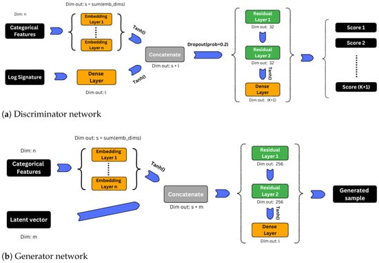
Figure 1.
Network architectures for discriminator and conditional generator.
Discriminator: Similar to [43], we aim for a discriminator D that takes into account class labels. We, however, propose a discriminator that returns a vector of raw scores with values in instead of estimating the probability that sample belongs to class , where class label 0 represents a sample produced by the generator. To do so, we construct a feedforward neural network D using tanh activation functions and residual layers.
Further, if given a real sample X containing both time series data and a categorical feature vector , we add a preprocessing step to extract meaningful information. We first augment the time series using a time augmentation, a lead-lag augmentation and an invisibility-reset augmentation. Second, we apply a piece-wise linear interpolation and finally compute the truncated log-signature of order four. These augmentations follow prior literature on log-signature modeling [11,36] and ensure the uniqueness of the log-signature, capture information on the quadratic variation in the process and add extra information about the starting point. The truncation of order four is a widely used compromise [36]: higher truncation orders capture more path information, but also increase dimensionality, which can reduce efficiency and stability. In this case, the dimension of a d-dimensional time series increases to . A detailed overview of possible path augmentation and their classification is given by [11]. Finally, in the generator, each categorical feature is passed through an embedding layer, mapping it to a vector with dimension . Concatenating the embeddings with the log-signature yields a final 271-dimensional representation for each transaction history. This is applied consistently to both real and synthetic samples.
For a given log-signature of length l and a vector of n categorical features, the discriminator network can be illustrated as Figure 1.
4.2. Loss Functions
Let be N unlabeled observations and be labeled real samples with class labels . We label generated data as class 0. For any given time series X, we form the augmented path and its truncated log-signature .
Discriminator: Our network outputs raw scores . For the discriminator we adopt a composite loss consisting of (i) a supervised classification part on labeled data, (ii) an unsupervised Wasserstein-style IPM term on real vs. generated samples and (iii) a gradient penalty ensuring 1-Lipschitz continuity of the network [42].
We use a fixed linear projection
which has operator norm to obtain the scalar critic .
On labeled real samples, we train the class scores with cross-entropy:
with
being the probability that sample belongs to class .
On unlabeled real and generated we minimize an Integral Probability Metric (IPM) estimated with the scalar critic :
By Kantorovich–Rubinstein duality [49], minimizing this objective is equivalent to maximizing the Wasserstein-1 distance in its dual formulation, restricted to the critic class . We enforce 1-Lipschitzness of via a gradient penalty [42] on interpolated features :
Note this applies the penalty to the scalar , avoiding ambiguity for vector outputs.
Finally, for a latent input z, a categorical vector , a sample X, scaling factors and and network weights and the loss function for the discriminator is defined as follows:
Together, these components can be interpreted as follows: performs empirical risk minimization on the scarce labeled data, enforces distributional alignment between real and generated log-signatures through an IPM, which is a standard technique in semi-supervised learning and domain adaptation [21,50] while a gradient penalty enforces the scalar critic remains 1-Lipschitz, a condition necessary for the IPM term to coincide with the Wasserstein–1 distance [42].
Generator: The generator is trained to generate samples that are classified as real by the scalar critic. Hence, for a latent input z, a categorical vector and network weights and , the loss for a mini-batch of samples is
Integral Probability Metric (IPM) and theoretical grounding: Our unlabeled objective can be formally understood as an Integral Probability Metric (IPM) in log-signature space. Given two distributions and a function class , the IPM is defined as
When is the set of 1-Lipschitz functions, equals the Wasserstein–1 distance by the Kantorovich–Rubinstein duality [49]. Our unlabeled loss takes the form
where is a scalar critic obtained by a fixed unit-norm projection T of the discriminator outputs. Since , is 1-Lipschitz whenever is. In practice, the supremum is approximated by optimizing under a gradient penalty that enforces 1-Lipschitz. Thus is an empirical estimate of restricted to this critic class, providing a principled Wasserstein-based IPM tailored to log-signature features rather than an ad-hoc design. Because T is fixed with , is 1-Lipschitz whenever is, ensuring the constraint is enforced. In summary, the discriminator’s composite loss can be interpreted as supervised risk minimization regularized by a Wasserstein discrepancy under a Lipschitz constraint.
Beyond Wasserstein-based IPMs, widely used distributional discrepancy measures, including MMD [51] or f-divergences [52] could be incorporated into our framework without changing the overall architecture. In the context of signature features, however, mainly MMD- and Wasserstein-based objectives have been explored: for example, refs. [53,54] introduced MMD with a signature kernel, for statistical tests and training generative models, while [36,48] integrate the Wasserstein-1 distance directly in signature space for time-series generation. These works highlight that both families of metrics are principled options in signature space. We adopt the Wasserstein formulation because it is well established in the literature, offers stable training dynamics, and aligns naturally with the geometric representation provided by log-signatures. A broader empirical comparison with alternative divergences, including signature-based MMD, remains an interesting direction for future work.
4.3. Posterior Sampling
To approximate the posterior over network weights, we follow the general Bayesian updating framework (see Section 3.3) and employ Stochastic Gradient Hamiltonian Monte Carlo (SGHMC), introduced in [44]. SGHMC is very closely related to momentum-based stochastic gradient descent (SGD), but injects calibrated Gaussian noise to simulate posterior samples while using mini-batches for scalability. Hence, parameter settings, such as learning rate and momentum terms, can be imported from standard optimizers.
Following [43], we set parameters and for the prior distributions and of the generator and discriminator weights, respectively. Initial weights and are drawn from these priors and updated with SGHMC (see Algorithm 1) using noise samples from the latent distribution and a mini-batch of real data samples . Posterior samples yield predictive distributions; for evaluation against baselines, we use the posterior mean prediction in Section 5.5.1, while uncertainty analyses rely on the full posterior predictive in Section 5.5.3. For clarity, we present one SGHMC iteration in Algorithm 1 using a standard momentum-based SGD. In practice, consistent with [43], we achieved more stable performance using ADAM-style momentum updates within the SGHMC framework. Choosing a prior distribution is a crucial part of Bayesian inference, which often relies on expert knowledge. We avoid any exogenous assumptions or domain expert knowledge and follow the Glorot normal initialization [55] to maintain a high information flow across layers. Network weights are randomly drawn from a centered normal distribution
with variance
with scaling factor g and fan in and fan out denoting the input and output dimensions of a network layer. As we use small layers down to 32 nodes, we choose to keep the variance reasonably small. Hyperparameters were adopted from commonly used settings in the literature, with minimal additional tuning of the learning rate. Based on this tuning study Table A2, we selected learning rates of 0.0001 for the generator and 0.005 for the discriminator in the final evaluation. The much higher learning rate for the discriminator D is based on the fact that it has to learn both classification and discrimination quickly, while the generator only learns through D’s signal [56]. The mini-batch size for both G and D is chosen as and For efficiency, we run one chain and train the generator/discriminator with alternating update steps using discriminator updates per one generator update for 1000 iterations. Convergence is monitored heuristically via stabilization of losses.
| Algorithm 1 One training epoch of SGHMC with SGD-style update with friction term , learning rate , and parallel running Markov Chains and previous posteriors samples and . |
|
Our approach constitutes an approximate Bayesian treatment of neural network weights via SGHMC. The resulting predictive distributions provide uncertainty estimates, which are central in fraud detection (e.g., for thresholding or human review). While a non-Bayesian variant may yield sharper point estimates, it would lack principled uncertainty estimates. We, therefore, regard Bayesian inference as an integral design choice, rather than an optional module for ablation.
5. Empirical Evaluation
5.1. Dataset and Preprocessing
The BankSim dataset is publicly available on Kaggle [15] and simulates financial transactions over approximately six months, based on data provided by a bank in Spain. Because access to real banking records is restricted by privacy and regulatory constraints, BankSim has become a common benchmark in fraud detection research, providing a common ground for methodological comparison. While not including any personal or legally sensitive customer information, it effectively replicates realistic transaction patterns, comprising 594,643 records, of which 7200 are fraudulent transactions. As a result, it serves as a robust foundation for developing and evaluating fraud detection models, serving both academic researchers and practitioners. The dataset contains ten columns, including seven categorical (customer, age, gender, zipcodeOri, merchant, zipMerchant and category), two continuous (step and amount) and a fraud label. Importantly, BankSim inherently exhibits irregular sampling, as customers’ transactions are executed at uneven intervals, and histories vary in length and frequency. This naturally evaluates an approach’s ability to handle missing and non-uniform temporal information.
In this paper, we do not work directly with single transaction features but rather formulate the fraud detection problem as a time series classification task. We, therefore, group transactions based on customer, resulting in a dataset of 4112 individual customers, of which 12 were excluded due to missing gender. Out of the remaining 4100 customers, 1479 contain fraudulent transactions. Each customer has conducted between 5 and 265 transactions of up to 8330 Euros. Since our sequential model requires a minimum transaction history before making predictions, we begin predicting after the first four transactions, ensuring each customer contributes at least one labeled sample. After an initial investigation, we observed that common transaction-level models such as Random Forest exhibit a disproportionately high dependence on the amount feature. In fact, merely scaling this single variable substantially changed the results, indicating a lack of robustness to variations such as different currencies (see Table A1). To address this and ensure fair comparability, we trained all models, except the sequential baseline, on our prepared log-signature data. This further allows each model to exploit the richer information contained in customers’ transaction histories, rather than relying on isolated single transactions.
We remove all identifiers for cardholders and merchants to encourage generalization and only keep a small set of raw features comparable to previous work [2,10]. We prepare the continuous features,
- step difference: Elapsed time since last transaction,
- amount: Amount of money involved in the transaction,
- and divide them by their maximum values in the train dataset, augment the path using a time augmentation, a lead-lag augmentation and an invisibility-reset augmentation and compute the log-signature of order four of the complete customer’s prefix history. Further, we add the categorical features:
- age: Most recent age category of the customer,
- gender: Most recent gender of the customer,
- risk level: Risk level of the customer. A customer’s risk level at time t is determined as the weighted average of its past transaction risk levels up to t, weighted by the sequential order of the transactions.
- Risk level categories are derived once from the training set and then applied consistently across both training and test sets. Transactions are grouped into five broad categories according to fraud prevalence: [0,2], (2,10], (10,30], (30,50], and (50,100] percent. This serves as a domain-driven dimensionality reduction step: instead of passing raw categorical identifiers, which would lead to a sparse feature space, we map them into a small number of stable, interpretable groups. The result is a categorical feature (level 1–5) reflecting typical expert practice in applied fraud detection, where transaction categories are routinely segmented into low- and high-risk bands.
5.2. Baseline Models
In addition to our proposed approach, we trained a diverse set of benchmark models for comparison. These include both traditional supervised machine learning classifiers and semi-supervised extensions. Following previous work in fraud detection [57], we selected nine representative baseline models covering linear, non-linear, tree-based and neural structures.
As classical benchmarks, we trained a Naive Bayes (NB), a logistic regression (LReg), a k-nearest neighbour (KNN) and a support vector machine (SVM). We further include a random forest as a widely used ensemble method in fraud detection and a fully supervised feed-forward neural network (FNN). The FNN uses the same architecture as our discriminator (see Figure 1), except the final layer produces two logits and the model is trained with standard cross-entropy loss. For a semi-supervised baseline, we include a self-training variant of logistic regression (LReg-SSL), utilizing the semi-supervised wrapper available in the scikit-learn Python package [58] and a Mean Teacher (MT) model [59] using the same architectures as our discriminator network.
While sequential models such as GRUs [60] are widely applied to sequential data, they face well-known limitations when histories are irregularly sampled and of variable length [61]. Their use typically requires ad hoc preprocessing (e.g., windowing, padding, time embeddings), or complex architectural adaptations. For completeness, we include a GRU baseline as a representative sequential model to provide a point of comparison. Peak performance from GRUs, however, typically requires substantial tuning and tailored design choices, which we explicitly leave for future work. Our focus here is on demonstrating that our Bayesian log-signature GAN naturally handles irregular sequences without imposing artificial structure.
5.3. Evaluation Procedure
Evaluating the performance of semi-supervised models requires special caution due to factors such as the selection of the labeled data points [14]. Ref. [62] provides guidelines for the realistic evaluation of semi-supervised models to guarantee unbiased and fair comparison results. This improved procedure includes splitting a fully labeled dataset into a small labeled dataset and a large unlabeled dataset with artificial unlabeling of randomly drawn samples. By varying the amount of labeled samples, we obtain insights into how performance decreases in very limited label regimes.
For our primary setting, we aim for a 90/10 split in and in a customer-disjoint manner, mirroring deployment conditions where models encounter previously unseen customers. To approximate stratification, we apply a greedy algorithm assigning customers, beginning with those having the highest number of fraud or non-fraud cases, but due to fraud clustering, this reduces test-set prevalence from around 1% to around 0.45%. To stress-test robustness, we, therefore, also report results using a stratified split in Appendix D, which preserves the global prevalence. Customer identifiers are excluded from the features, so the models cannot directly exploit customer identity. Together, these results illustrate both a realistic deployment case (customer-disjoint) and the general performance potential of the models (stratified), ensuring that our conclusions remain robust across alternative splitting strategies.
We train each model on with varying amounts of labeled samples Model performance is compared on . To stress-test robustness against unfavorably selected labeled samples, we repeat the unlabeling step five times, which is also in line with [18]. All reported means and standard deviations are computed across these five unlabelings, capturing sensitivity to the choice of labeled subset rather than training stochasticity or test set uncertainty.
5.4. Performance Metrics
Performance evaluation is particularly important for highly imbalanced datasets such as those encountered in fraud detection [1]. In this setting, only a very small fraction of transactions can be manually investigated or automatically blocked, meaning that model performance in the head of the ranked distribution is of primary interest. Recent work by [63] has shown that the choice of evaluation methodology often has a greater impact on reported performance than model complexity itself.
In this work, we adopt a comprehensive set of evaluation metrics combining standard global measures for imbalanced data with domain-specific, cost-sensitive metrics. The global measures include area under the precision recall curve (PR-AUC), macro F1 score and cross-entropy loss. Although providing an initial overview of overall performance, such global metrics are less informative in practice because they aggregate over thresholds that are rarely relevant for real-world operation [1]. To address these limitations, and in line with common practice in information retrieval [64] and fraud detection research [1,10], we complement them with the head metrics Precision@K, Recall@K, partial PR-AUC, and Expected Cost@K to directly reflect operational constraints. Let TP, FP, TN, FN denote the number of true positives, false positives, true negatives and false negatives, respectively. Then precision and recall are defined as and . The F1 score combines them as
The macro F1 score is obtained by averaging the F1 scores for the two classes (fraud and non-fraud), ensuring equal importance of both despite the class imbalance. The PR curve plots precision as a function of recall and PR-AUC, denoting the area under this curve, summarizing performance across thresholds.
Beyond point classification, we also assess the quality of predictive distributions using the cross-entropy loss. For N transactions, it is given by
where denotes the predicted probability that transaction is fraudulent.
To focus on the operationally most relevant part of the distribution, we evaluate head metrics with respect to the top of transactions ranked by predicted fraud probability. Particularly,
where and denote the number of true and false positives within the top and denotes the false negatives outside of this subset. We additionally employ partial PR-AUC, a restricted variant of standard PR-AUC. Instead of integrating precision over the full recall range , partial PR-AUC is computed only over a recall interval for fixed as,
where denotes the precision at recall level s. This restriction reflects the reality that financial institutions rarely operate at very high recall values due to limited investigation capacity. By focusing on realistic recall ranges, partial PR-AUC better reflects the ranking quality of models in the operational regime.
Finally, to incorporate financial impact, we adopt Expected Cost@K in line with cost-sensitive learning frameworks [10,65]. A false negative (missed fraud) is assigned the full amount (), representing reimbursement to the customer, whereas a false positive (legitimate transaction flagged as fraud) is assigned a fixed fraction of the transaction, representing the lost transaction fees and operational overhead. For transaction amounts this yields,
This cost-based measure enables direct comparison of models in terms of their business impact, complementing the global statistical metrics.
5.5. Numerical Results
5.5.1. Discriminative Performance Evaluation
We evaluate the performance of all trained models using labeled subsets of size , corresponding to 0.5%, 0.75%, 1%, 2.5% and 5% of available training samples. The labeled subsets were randomly selected while preserving the original class distribution, resulting in fraudulent transactions, respectively. To obtain a global comparison across different training sizes, we report three complementary metrics, namely macro F1, PR-AUC and cross-entropy loss (CEL) (see Section 5.4). These capture balanced classification performance across classes, ranking quality under class imbalance and probabilistic calibration. As expected, we observe higher volatility across all metrics and models for smaller labeled subsets, with performance stabilizing as increases. Further, the fully supervised neural network (FNN) displays a steeper performance curve, gradually catching up, and in some cases surpassing our semi-supervised model as the amount of labeled data grows and the benefit of semi-supervised learning diminishes.
Macro F1 results are reported in Table 1. Across all sample sizes, either our proposed approach or the FNN achieved the highest scores.

Table 1.
Macro F1 scores across models and training sizes. Values are mean (standard deviation). Best values are in bold.
In terms of CEL, our model consistently outperformed all benchmark models across all labeled training sizes (Table 2). However, we again observe a narrowing gap as the FNN benefits from larger datasets.
Table 2.
Cross-entropy loss across models and training sizes. Values are mean (standard deviation). Best values per row are in bold.
For PR-AUC, our model achieved the highest scores for low amounts of labeled data, whereas FNN and RF take over when more labeled training data become available (see Table 3).
Table 3.
PR-AUC across models and training sizes. Values are mean (standard deviation). Best values per row are in bold.
While the given global metrics provide a useful statistical model comparison, in financial fraud detection, the expected financial cost of errors is often more relevant in practice. Therefore, we adopt Expected Cost@K as our primary domain-specific metric, where K controls the fraction of transactions to be blocked or investigated. A visual comparison for is given in Figure 2. Our model achieved the lowest expected cost, reducing financial cost relative to the statistically strong RF baseline by approximately 24–44% across labeled training sizes. Moreover, our approach exhibits the smallest variance across unlabelings, indicating higher generalization ability and stability compared with baselines. A detailed comparison for multiple values of K is reported in Table A3.
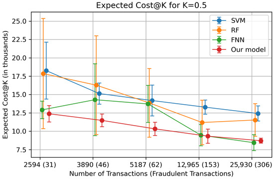
Figure 2.
Expected Cost@K for K = 0.5 for various amounts of labeled samples {2594, 3890, 5187, 12,966, 25,930}. Dots represent mean over 5 repetitions where labels were randomly withheld to simulate partially labeled training sets. Vertical error bars are the standard deviation across repetitions. Dots are jittered on the x-axis to avoid overlapping error bars. Values are presented in thousands. Numbers in parentheses on the x-axis indicate the number of fraudulent transactions within the labeled data.
For the main evaluation, we fix the penalty weights for false negatives and false positives to and , respectively. To assess robustness, we additionally vary across four alternative settings. The full results, including comparisons across labeled training sizes and multiple K values, are reported in Figure A1, where the relative ranking remains stable across settings.
We further report Precision@K for in Table 4. Our model achieved higher scores for limited labeled sample sizes, whereas the FNN and RF gradually overtook as more labeled samples became available. Full results for additional k values are presented in Table A4.
Table 4.
Precision@K for for different models and training sizes. Values are mean (standard deviation). Bold numbers indicate the best performance per row.
Similarly, Recall@K for is reported in Table 5. Our model performs best for limited labeled sample sizes, while the FNN and RF surpass it once larger sample sizes are used. Additional Recall@K results are given in Table A5.
Table 5.
Recall@K for for different models and training sizes. Values are mean (standard deviation). Bold numbers indicate the best performance per row.
Finally, partial PR-AUC with a recall threshold is reported in Table 6. Here, our model achieved the best performance across all sample sizes except the largest, where the FNN wins. Extended results for different recall thresholds are provided in Table A6.
Table 6.
Partial PR-AUC at across different training sizes. Values are mean (standard deviation). Bold numbers indicate the best performance per row.
While head metrics emphasize the practically relevant head of the ranked distribution, relying solely on point estimates may still be misleading. A single prediction may appear highly confident, placing a transaction high in the ranking, yet posterior sampling may reveal substantial uncertainty of the underlying model and correct such spurious point estimates and push uncertain cases lower in the ranking. This motivates the following analysis of Bayesian uncertainty, where predictive distributions rather than single predictions provide a more robust basis for decision-making.
5.5.2. Runtime and Scalability
All experiments were conducted on Kaggle’s free Tesla T4 and P100 GPUs, without access to high-performance clusters. On the BankSim dataset with about 600k transactions approximate wall-clock training times for all main models are illustrated in Table 7. For comparability, runtimes measure only the training loop with limited loss logging; data preprocessing (e.g., log-signature computation) is excluded. Despite the Bayesian framework, training remains efficient due to the shallow architecture of both generator and discriminator, highlighting practical deployability. Codes for reproducing the results and figures for this paper are available on https://github.com/DavidHirnschall/logsig-bayesian-gan (accessed on 28 August 2025).
Table 7.
Training runtimes per model (approximate wall-clock times).
5.5.3. Uncertainty Evaluation
To assess predictive uncertainty of our Bayesian approach, we approximate the predictive distribution for each transaction over fraud probability from SGHMC samples and summarize uncertainty by the posterior interval width, e.g., the 90% interval width In practice, one may call a prediction uncertain if the classification threshold lies within the interval , as it returns mixed classification signals. In the quantitative evaluation below, we use the continuous score
For comparison, we additionally evaluate (i) the maximum softmax probability (MSP), i.e., , (ii) posterior standard deviation across SGHMC samples and (iii) mutual information (MI) between predictions and model posterior, which captures epistemic uncertainty. Given M posterior predictive distributions , the posterior predictive distribution is . Then the MI is
where is the categorical entropy.
To test whether uncertainty identifies mistakes in predictions, we treat misclassifications as the positive class, compute the ROC curve using the uncertainty scores as the ranking variable, and report the area under the ROC curve (AUROC) in Table 8. While the ROC curve plots the true positive rate against the false positive rate across thresholds, the AUROC gives the probability that an error receives a higher uncertainty score than a correct prediction by
with 0.5 indicating random ranking and higher scores indicating better performance.
Table 8.
AUROC values for different uncertainty measures across labeled sample sizes . Values are mean (standard deviation). Best per row in bold.
With scarce labels, epistemic uncertainty dominates, meaning the posterior over weights diffuses and SGHMC draws disagree, resulting in broad predictive intervals. Interval-based uncertainty scores directly reflect this behavior and separate wrong from correct predictions more effectively. As the number of labeled samples grows, posterior predictions concentrate and intervals shrink (see Figure 3). Misclassifications are less driven by model uncertainty and more by predictions near the decision threshold. Point estimators become better calibrated, so simple uncertainty scores derived from posterior mean, e.g., MSP gain importance. This pattern reflects the intuition that more data reduces posterior variance and tightens predictive intervals. While intervals are not always the best in ranking errors, they remain highly interpretable and provide a direct probability range for decision rules, making them particularly appealing in fraud detection.
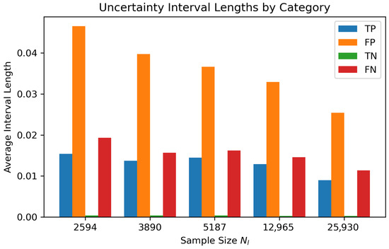
Figure 3.
Average 90% uncertainty interval width over five unlabelings by outcome (TP/FP/TN/FN) across labeled sample sizes . Misclassified instances (FP/FN) are consistently more uncertain than correct ones (TP/TN).
Further, we categorize transactions in true positive (TP), false positive (FP), true negative (TN) and false negative (FN) via the posterior mean prediction . Figure 3 displays average 90% interval widths over five unlabelings for each category (TP, FP, TN, FN) and across labeled sample sizes. Misclassified instances (FP and FN) consistently exhibit a substantially larger uncertainty than correctly classified ones (TP and TN). This systematic separation confirms that interval-based measures capture epistemic uncertainty in a way that directly aligns with predictive reliability.
Finally, Figure 4 shows posterior distributions for four representative transactions (one per outcome category) with decision threshold overlaid by the uncertainty interval. Among samples labeled as fraud, misclassified FPs tend to show broader posteriors, hence higher uncertainty, with more weight in the left tail. Among transactions labeled as non-fraud, misclassified FNs exhibit wider predictive posteriors with heavier right tails. These pattern reflects epistemic uncertainty beyond the point estimate .
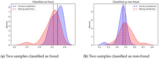
Figure 4.
Predictive distributions for four uncertain predictions, one from each category (TP, FP, TN, FN).
5.6. Fairness Across Demographic Groups
Since age and gender are included as features, we evaluated subgroup performance in the test set to assess fairness. Figure 5 presents results for labeled data (5187 samples) for our model, SVM and RF. Performance differences across gender and age groups largely reflect underlying fraud prevalence and group size, rather than systematic bias introduced by the model. Groups with higher fraud prevalence naturally show higher F1, PR-AUC and expected cost due to the greater number of positive cases. Importantly, relative model rankings remain consistent across groups and our approach improves calibration and precision-recall trade-offs across most groups. This indicates that no particular group is systematically disadvantaged and the similar behavior of baseline models further supports the interpretation that observed differences are data-driven rather than model-driven.
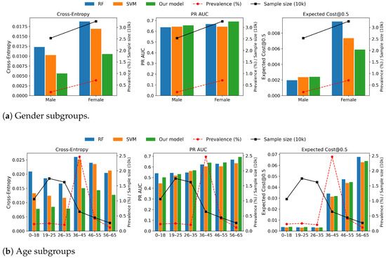
Figure 5.
Subgroup performance for labeled transactions (5187 samples). Each grouping is evaluated on three metrics (cross-entropy, PR-AUC and Expected Cost@0.5). Bars correspond to RF, SVM and our model. The dashed red line indicates subgroup fraud prevalence in % and solid black line shows samples in tens of thousands. Differences between subgroups align with prevalences and sample sizes, indicating disparities are data-driven rather than model-driven.
Nevertheless, the inclusion of demographic features must be handled with care. Even if statistically predictive, they can introduce or reinforce unfair outcomes at the individual level. A practical safeguard is leveraging predictive uncertainty, where uncertain cases can be flagged for human inspection. Finally, subgroup results for small populations should be interpreted cautiously, as a limited sample size naturally leads to high variance. Detailed results across age and gender groups for RF, SVM and our model are reported in Table A7 and Table A8.
6. Conclusions and Discussion
In this paper, we introduced a novel deep generative semi-supervised approach for time series classification that leverages conditional GANs, Bayesian inference, and log-signatures to address core challenges in financial fraud detection: irregularly sampled data of varying length, limited labeled samples and the need for probabilistic predictions with uncertainty quantification. Log-signatures provide a principled way to encode transaction histories of variable length, enabling robust learning where other sequence models struggle.
To provide a comprehensive performance assessment, we combined global statistical metrics (macro F1, PR-AUC, cross-entropy loss) with domain-specific head metrics (Precision@K, Recall@K, partial PR-AUC, Expected Cost@K). This dual evaluation framework reflects both overall statistical performance and real-world business impact, where only a small fraction of transactions can be reviewed. Our empirical evaluation on the BankSim dataset demonstrated that our proposed approach outperforms established baselines in the low-data regime, with particularly strong gains in cost-based performance at realistic operational settings, achieving up to 44% lower Expected Cost@K than strong statistical performers such as random forest in typical operational regimes. While fully supervised neural networks close the performance gap as more labeled samples become available, our approach maintains a clear advantage when labeled data are scarce.
Another key contribution lies in uncertainty quantification. By placing a distribution over network weights, our Bayesian framework produces predictive distributions rather than point estimates, allowing calibrated confidence intervals. Misclassified samples were shown to exhibit consistently higher uncertainty, highlighting the importance of uncertainty-aware predictions in high-risk domains where wrong decisions carry substantial cost. In addition, we evaluated subgroup performance by age and gender, finding that observed performance differences largely reflect prevalence and sample size rather than systematic bias introduced by the model. Relative model rankings remained stable across subgroups, suggesting that no group is systematically disadvantaged.
Nonetheless, limitations remain. Our approach relies on transaction histories, making predictions for new or low-activity customers challenging. Moreover, fraud detection assumes that fraud breaks behavioral patterns, which may fail in cases of repeated fraud resembling past activity. Finally, our evaluation relies on the BankSim dataset. While widely used in fraud detection for its realism, it remains synthetic, and future work should extend validation to real-world datasets as access becomes possible. As with most data-driven systems, model generalization depends on representative training data and evolving fraud tactics will require continuous retraining.
Several avenues for future research extend naturally from this work. First, extending evaluation to real-world datasets and in production environments offers the opportunity to confirm findings under operational constraints. Second, incorporating additional data modalities, such as customer demographics, merchant information, or network structures, could enhance the detection of rare or adaptive fraud cases. Third, fairness and interpretability remain important directions: while subgroup analyses suggest that performance differences primarily reflect data prevalence, future work should explore fairness-aware training objectives and explainable prediction mechanisms to strengthen trust in deployment. Finally, applying the approach to other domains, such as healthcare, is a natural next step to test the generalization of our approach to broader time series classification tasks beyond fraud detection.
Overall, our findings demonstrate that semi-supervised Bayesian generative models, combined with log-signatures for temporal feature encoding, can effectively handle variable-length sequences of irregular sampling frequencies while providing robust, uncertainty-aware decision support. This synergy offers tangible benefits for fraud detection and broader time series classification tasks.
Funding
This research received no external funding.
Data Availability Statement
The data presented in this study are openly available in https://www.kaggle.com/datasets/ealaxi/banksim1 (accessed on 28 August 2025).
Conflicts of Interest
The author declares no conflicts of interest.
Appendix A. Full Experimental Results
Table A1 shows the effect of scaling the transaction amount feature on classical baselines. Across all sizes of labeled training sets, performance drops dramatically when scaling is applied. Naive Bayes collapses to random-like performance with a macro F1 score of about 0.1, logistic regression suffers orders of magnitude worse calibration (cross-entropy loss increased from under 0.1 to over 5) and PR-AUC values shrink significantly. This highlights the sensitivity to raw values, indicating that naive preprocessing can destroy predictive signal.
Table A1.
Performance of baseline models with and without scaling of the amount feature. Values are means across random unlabelings.
Table A1.
Performance of baseline models with and without scaling of the amount feature. Values are means across random unlabelings.
| Metric | NB | LReg | LReg-SSL | KNN | SVM | RF | |||||||
|---|---|---|---|---|---|---|---|---|---|---|---|---|---|
| Unscaled | Scaled | Unscaled | Scaled | Unscaled | Scaled | Unscaled | Scaled | Unscaled | Scaled | Unscaled | Scaled | ||
| 2595 | Macro F1 | 0.640 | 0.013 | 0.532 | 0.215 | 0.505 | 0.376 | 0.536 | 0.499 | 0.640 | 0.497 | 0.691 | 0.558 |
| CEL | 1.332 | 33.987 | 0.048 | 8.163 | 0.094 | 5.105 | 0.333 | 0.373 | 0.048 | 0.062 | 0.046 | 0.488 | |
| PR-AUC | 0.498 | 0.506 | 0.155 | 0.558 | 0.194 | 0.577 | 0.163 | 0.035 | 0.417 | 0.082 | 0.661 | 0.277 | |
| 3893 | Macro F1 | 0.639 | 0.013 | 0.530 | 0.200 | 0.510 | 0.314 | 0.548 | 0.502 | 0.692 | 0.508 | 0.725 | 0.612 |
| CEL | 1.371 | 33.992 | 0.047 | 8.509 | 0.087 | 6.926 | 0.316 | 0.365 | 0.042 | 0.062 | 0.044 | 0.493 | |
| PR-AUC | 0.503 | 0.506 | 0.187 | 0.548 | 0.236 | 0.548 | 0.214 | 0.056 | 0.500 | 0.166 | 0.683 | 0.355 | |
| 5190 | Macro F1 | 0.641 | 0.013 | 0.531 | 0.366 | 0.515 | 0.329 | 0.548 | 0.502 | 0.728 | 0.515 | 0.742 | 0.530 |
| CEL | 1.334 | 33.992 | 0.045 | 5.117 | 0.082 | 6.125 | 0.301 | 0.361 | 0.035 | 0.061 | 0.044 | 0.507 | |
| PR-AUC | 0.505 | 0.506 | 0.209 | 0.610 | 0.254 | 0.557 | 0.239 | 0.062 | 0.580 | 0.229 | 0.696 | 0.369 | |
| 12,973 | Macro F1 | 0.643 | 0.013 | 0.580 | 0.152 | 0.548 | 0.338 | 0.600 | 0.511 | 0.800 | 0.520 | 0.817 | 0.471 |
| CEL | 1.313 | 33.998 | 0.042 | 14.521 | 0.067 | 4.416 | 0.265 | 0.344 | 0.031 | 0.060 | 0.040 | 0.596 | |
| PRAUC | 0.505 | 0.506 | 0.300 | 0.528 | 0.338 | 0.573 | 0.359 | 0.100 | 0.663 | 0.212 | 0.754 | 0.440 | |
| 25,946 | Macro F1 | 0.645 | 0.013 | 0.617 | 0.229 | 0.560 | 0.225 | 0.644 | 0.525 | 0.822 | 0.522 | 0.837 | 0.597 |
| CEL | 1.295 | 33.997 | 0.038 | 6.422 | 0.057 | 11.258 | 0.242 | 0.329 | 0.029 | 0.060 | 0.038 | 0.546 | |
| PR-AUC | 0.504 | 0.506 | 0.384 | 0.568 | 0.407 | 0.524 | 0.443 | 0.146 | 0.688 | 0.191 | 0.772 | 0.518 | |
Following [56], who highlights the need for a higher learning rate in the discriminator, as it must adapt rapidly to both classification and discrimination while the generator only learns indirectly through the discriminator’s feedback, we fixed the generator’s learning rate to a standard and tuned the discriminator’s learning rate as a multiple thereof. We performed a small calibration study using three multipliers (1, 10, 50) across three labeled sample sizes and three random unlabelings. For each configuration, we report mean and standard deviation for Expected Cost@K with , macro F1 and cross-entropy loss. Table A2 shows that achieved a comparable mean performance to , with a modest increase in variability. As higher learning rates typically accelerate convergence, and since our main results average over five random unlabelings, which provides more stability, we opt for the higher learning rate of 0.005 for the discriminator. This calibration was conducted on a stratified train/test split, as we aim for the best possible generalization ability.
Table A2.
Performance of our model under different learning rates. Values are reported as mean (standard deviation) across random unlabelings.
Table A2.
Performance of our model under different learning rates. Values are reported as mean (standard deviation) across random unlabelings.
| Learning Rate | Sample Size | Expected Cost | Macro F1 | Cross-Entropy Loss |
|---|---|---|---|---|
| 0.0001 | 2595 | 199,930 (12,345) | 0.557 (0.030) | 0.054 (0.005) |
| 5190 | 166,067 (6721) | 0.600 (0.019) | 0.043 (0.001) | |
| 25,946 | 152,893 (650) | 0.606 (0.008) | 0.040 (0.000) | |
| 0.001 | 2595 | 126,633 (29,351) | 0.702 (0.035) | 0.071 (0.016) |
| 5190 | 72,263 (4378) | 0.838 (0.003) | 0.026 (0.001) | |
| 25,946 | 66,377 (357) | 0.859 (0.003) | 0.020 (0.000) | |
| 0.005 | 2595 | 130,644 (39,320) | 0.684 (0.053) | 0.065 (0.017) |
| 5190 | 72,251 (3609) | 0.832 (0.000) | 0.027 (0.001) | |
| 25,946 | 66,648 (632) | 0.859 (0.004) | 0.020 ( 0.000) |
For completeness, we report the full set of domain-specific evaluation metrics across all investigated values of K. Specifically, we evaluated Precision@K, Recall@K and Expected Cost@K for and partial PR-AUC for recall thresholds .
Table A3 presents the expected cost for all models and labeled training sample sizes across different values of K, directly reflecting the financial impact of false predictions. This metric provides the most application-relevant evaluation.
Table A3.
Expected Cost@K for different models, training sizes and values of K. Values reported as mean (standard deviation) in thousands. Bold values indicate the best result per row.
Table A3.
Expected Cost@K for different models, training sizes and values of K. Values reported as mean (standard deviation) in thousands. Bold values indicate the best result per row.
| K | NB | LReg | LReg-SSL | KNN | SVM | RF | FNN | Our Model | GRU | MT | |
|---|---|---|---|---|---|---|---|---|---|---|---|
| 0.1 | 2594 | 110.4 (10.8) | 89.1 (5.4) | 88.6 (9.5) | 107.4 (8.7) | 61.3 (3.2) | 75.0 (7.5) | 57.7 (2.0) | 57.2 (1.2) | 86.6 (8.3) | 94.4 (19.7) |
| 3890 | 116.4 (3.9) | 84.2 (4.8) | 81.6 (5.9) | 107.8 (8.7) | 57.9 (1.0) | 72.3 (4.2) | 64.0 (14.6) | 60.8 (9.3) | 91.8 (3.0) | 79.4 (6.3) | |
| 5187 | 104.9 (6.5) | 82.1 (4.4) | 76.1 (1.8) | 103.8 (9.6) | 58.3 (1.2) | 73.1 (5.4) | 67.4 (12.5) | 57.5 (2.0) | 92.2 (8.2) | 78.0 (9.3) | |
| 12,965 | 101.7 (7.5) | 76.0 (1.1) | 68.3 (1.5) | 97.9 (6.4) | 57.0 (0.6) | 70.8 (6.1) | 66.3 (13.1) | 56.8 (9.3) | 90.2 (9.3) | 76.8 (9.1) | |
| 25,930 | 104.2 (5.4) | 69.3 (1.3) | 66.1 (1.7) | 97.4 (13.3) | 56.9 (0.4) | 67.0 (4.2) | 64.8 (11.1) | 56.1 (0.4) | 88.7 (3.2) | 74.7 (5.7) | |
| 0.2 | 2594 | 94.8 (11.8) | 81.3 (6.2) | 80.2 (8.9) | 100.4 (4.6) | 41.5 (8.2) | 46.4 (4.0) | 31.2 (1.1) | 31.0 (0.7) | 59.2 (16.6) | 75.4 (5.1) |
| 3890 | 98.0 (12.5) | 72.5 (7.4) | 71.7 (3.8) | 90.7 (11.7) | 35.0 (2.3) | 47.2 (4.7) | 39.1 (13.9) | 33.6 (5.2) | 71.3 (7.9) | 69.7 (3.4) | |
| 5187 | 81.0 (8.4) | 66.4 (4.4) | 66.2 (4.5) | 93.0 (11.2) | 33.8 (1.8) | 45.1 (4.9) | 41.1 (10.6) | 31.6 (1.3) | 61.7 (10.2) | 62.3 (5.6) | |
| 12,965 | 77.3 (12.9) | 58.0 (2.1) | 55.2 (3.8) | 84.7 (7.3) | 32.4 (0.8) | 42.1 (3.0) | 40.0 (12.3) | 30.7 (1.3) | 62.0 (17.5) | 62.8 (8.3) | |
| 25,930 | 80.6 (10.7) | 53.9 (0.5) | 47.3 (2.3) | 76.8 (7.4) | 32.1 (0.6) | 40.7 (1.2) | 33.7 (3.9) | 30.0 (0.8) | 60.7 (8.8) | 64.8 (3.2) | |
| 0.5 | 2594 | 56.3 (22.9) | 61.1 (7.4) | 64.0 (13.1) | 95.7 (9.4) | 18.3 (3.9) | 17.9 (7.5) | 12.9 (1.2) | 12.4 (1.1) | 20.4 (5.3) | 60.6 (8.9) |
| 3890 | 60.8 (16.6) | 56.7 (7.4) | 53.3 (1.7) | 83.8 (12.9) | 15.1 (1.4) | 16.3 (6.7) | 14.3 (4.9) | 11.5 (0.9) | 26.3 (3.3) | 59.4 (6.5) | |
| 5187 | 33.4 (19.8) | 51.6 (1.8) | 49.6 (2.3) | 79.7 (16.6) | 14.2 (2.1) | 13.9 (4.7) | 13.7 (2.5) | 10.3 (0.9) | 28.9 (10.9) | 47.6 (3.1) | |
| 12,965 | 20.4 (9.8) | 48.3 (1.4) | 35.8 (2.8) | 66.5 (17.1) | 13.3 (1.0) | 11.2 (3.0) | 9.5 (1.5) | 9.3 (1.0) | 27.2 (10.5) | 39.6 (3.7) | |
| 25,930 | 17.6 (4.2) | 36.6 (1.9) | 27.4 (1.6) | 53.6 (10.5) | 12.4 (1.0) | 11.5 (2.2) | 8.4 (1.1) | 8.7 (0.3) | 21.8 (2.8) | 34.3 (5.5) | |
| 1.0 | 2595 | 10.9 (4.9) | 58.2 (5.3) | 58.0 (15.4) | 93.9 (9.9) | 13.1 (3.8) | 6.6 (1.5) | 10.0 (0.8) | 9.3 (1.1) | 13.7 (3.4) | 58.3 (10.1) |
| 3890 | 8.6 (0.6) | 53.6 (4.7) | 49.3 (2.4) | 82.7 (13.3) | 11.1 (2.1) | 6.3 (2.2) | 10.1 (0.9) | 8.2 (1.0) | 13.5 (1.8) | 53.0 (12.4) | |
| 5187 | 8.6 (0.6) | 49.6 (0.6) | 46.6 (1.6) | 79.4 (16.7) | 10.0 (1.8) | 5.3 (0.9) | 9.6 (0.6) | 7.7 (1.3) | 15.4 (2.2) | 43.5 (6.4) | |
| 12,965 | 8.3 (0.9) | 46.9 (0.8) | 31.1 (2.0) | 66.4 (17.2) | 9.6 (0.7) | 5.8 (1.4) | 7.2 (1.0) | 7.2 (1.2) | 15.3 (2.9) | 34.2 (4.7) | |
| 25,930 | 8.1 (0.2) | 34.1 (1.3) | 23.9 (2.8) | 53.6 (10.6) | 9.6 (0.8) | 5.5 (1.1) | 6.7 (0.8) | 7.0 (0.6) | 13.8 (3.6) | 26.0 (1.7) |
Table A4 reports Precision@K across the same setting. It shows how effective each model is in identifying true fraud within the top-K% ranked transactions. This is especially critical to minimize unnecessary investigations.
Table A4.
Precision@K for different models, training sizes and values of K. Values reported as mean (standard deviation). Bold values indicate the best result per row.
Table A4.
Precision@K for different models, training sizes and values of K. Values reported as mean (standard deviation). Bold values indicate the best result per row.
| K | NB | LReg | LReg-SSL | KNN | SVM | RF | FNN | Our Model | GRU | MT | |
|---|---|---|---|---|---|---|---|---|---|---|---|
| 0.1 | 2594 | 0.524 (0.32) | 0.690 (0.03) | 0.645 (0.15) | 0.486 (0.22) | 0.955 (0.02) | 0.955 (0.03) | 0.966 (0.00) | 0.966 (0.00) | 0.810 (0.16) | 0.497 (0.18) |
| 3890 | 0.352 (0.22) | 0.690 (0.02) | 0.710 (0.09) | 0.355 (0.15) | 0.966 (0.00) | 0.945 (0.05) | 0.969 (0.01) | 0.966 (0.00) | 0.797 (0.10) | 0.617 (0.16) | |
| 5187 | 0.638 (0.23) | 0.686 (0.01) | 0.783 (0.09) | 0.383 (0.14) | 0.962 (0.01) | 0.938 (0.03) | 0.966 (0.00) | 0.966 (0.00) | 0.803 (0.15) | 0.666 (0.14) | |
| 12,965 | 0.586 (0.09) | 0.700 (0.02) | 0.914 (0.07) | 0.528 (0.17) | 0.966 (0.00) | 0.962 (0.04) | 0.972 (0.01) | 0.966 (0.00) | 0.831 (0.09) | 0.779 (0.14) | |
| 25,930 | 0.655 (0.16) | 0.845 (0.07) | 0.948 (0.00) | 0.569 (0.10) | 0.966 (0.00) | 0.972 (0.02) | 0.969 (0.01) | 0.966 (0.00) | 0.855 (0.07) | 0.779 (0.10) | |
| 0.2 | 2594 | 0.453 (0.21) | 0.574 (0.02) | 0.484 (0.16) | 0.381 (0.20) | 0.848 (0.09) | 0.869 (0.05) | 0.969 (0.02) | 0.978 (0.01) | 0.745 (0.14) | 0.472 (0.15) |
| 3890 | 0.429 (0.23) | 0.634 (0.04) | 0.591 (0.04) | 0.383 (0.19) | 0.926 (0.06) | 0.826 (0.05) | 0.955 (0.04) | 0.978 (0.01) | 0.716 (0.11) | 0.486 (0.12) | |
| 5187 | 0.636 (0.13) | 0.664 (0.04) | 0.631 (0.04) | 0.350 (0.17) | 0.938 (0.06) | 0.836 (0.05) | 0.960 (0.03) | 0.976 (0.01) | 0.743 (0.11) | 0.621 (0.07) | |
| 12,965 | 0.648 (0.16) | 0.753 (0.04) | 0.759 (0.05) | 0.445 (0.14) | 0.957 (0.01) | 0.900 (0.03) | 0.971 (0.02) | 0.981 (0.00) | 0.776 (0.11) | 0.653 (0.08) | |
| 25,930 | 0.621 (0.10) | 0.814 (0.01) | 0.831 (0.01) | 0.538 (0.11) | 0.960 (0.01) | 0.924 (0.03) | 0.981 (0.00) | 0.983 (0.00) | 0.783 (0.07) | 0.619 (0.00) | |
| 0.5 | 2594 | 0.429 (0.16) | 0.420 (0.02) | 0.318 (0.11) | 0.175 (0.11) | 0.571 (0.07) | 0.596 (0.07) | 0.616 (0.03) | 0.628 (0.02) | 0.543 (0.06) | 0.277 (0.11) |
| 3890 | 0.388 (0.12) | 0.419 (0.04) | 0.413 (0.03) | 0.189 (0.09) | 0.592 (0.02) | 0.610 (0.07) | 0.629 (0.04) | 0.641 (0.02) | 0.517 (0.04) | 0.282 (0.07) | |
| 5187 | 0.550 (0.07) | 0.436 (0.03) | 0.431 (0.03) | 0.206 (0.12) | 0.599 (0.04) | 0.634 (0.07) | 0.631 (0.03) | 0.654 (0.02) | 0.494 (0.05) | 0.374 (0.07) | |
| 12,965 | 0.598 (0.04) | 0.462 (0.02) | 0.494 (0.01) | 0.268 (0.13) | 0.597 (0.02) | 0.688 (0.02) | 0.670 (0.03) | 0.662 (0.02) | 0.524 (0.04) | 0.470 (0.02) | |
| 25,930 | 0.614 (0.02) | 0.512 (0.01) | 0.548 (0.01) | 0.349 (0.07) | 0.611 (0.01) | 0.700 (0.02) | 0.674 (0.01) | 0.659 (0.01) | 0.539 (0.03) | 0.499 (0.04) | |
| 1.0 | 2594 | 0.358 (0.02) | 0.227 (0.01) | 0.191 (0.07) | 0.093 (0.06) | 0.325 (0.03) | 0.366 (0.02) | 0.347 (0.01) | 0.353 (0.01) | 0.314 (0.03) | 0.149 (0.05) |
| 3890 | 0.364 (0.01) | 0.233 (0.01) | 0.233 (0.01) | 0.098 (0.05) | 0.332 (0.02) | 0.379 (0.02) | 0.352 (0.02) | 0.364 (0.02) | 0.319 (0.02) | 0.167 (0.06) | |
| 5187 | 0.362 (0.01) | 0.236 (0.00) | 0.234 (0.01) | 0.105 (0.06) | 0.337 (0.02) | 0.390 (0.01) | 0.357 (0.01) | 0.367 (0.01) | 0.312 (0.02) | 0.206 (0.04) | |
| 12,965 | 0.366 (0.01) | 0.243 (0.00) | 0.272 (0.00) | 0.136 (0.07) | 0.337 (0.01) | 0.393 (0.01) | 0.378 (0.01) | 0.374 (0.01) | 0.314 (0.02) | 0.257 (0.01) | |
| 25,930 | 0.367 (0.00) | 0.271 (0.00) | 0.298 (0.01) | 0.176 (0.04) | 0.342 (0.00) | 0.404 (0.01) | 0.378 (0.01) | 0.371 (0.01) | 0.317 (0.02) | 0.286 (0.01) |
Table A5 provides Recall@K results, reflecting the share of frauds captured within the top-K%.
Table A5.
Recall@K for different models, training sizes and values of K. Values reported as mean (standard deviation). Bold values indicate the best result per row.
Table A5.
Recall@K for different models, training sizes and values of K. Values reported as mean (standard deviation). Bold values indicate the best result per row.
| K | NB | LReg | LReg-SSL | KNN | SVM | RF | FNN | Our Model | GRU | MT | |
|---|---|---|---|---|---|---|---|---|---|---|---|
| 0.1 | 2594 | 0.109 (0.07) | 0.144 (0.01) | 0.135 (0.03) | 0.101 (0.05) | 0.199 (0.01) | 0.199 (0.01) | 0.201 (0.00) | 0.201 (0.00) | 0.169 (0.03) | 0.104 (0.04) |
| 3890 | 0.073 (0.05) | 0.144 (0.00) | 0.148 (0.02) | 0.074 (0.03) | 0.201 (0.00) | 0.197 (0.01) | 0.202 (0.00) | 0.201 (0.00) | 0.166 (0.02) | 0.129 (0.03) | |
| 5187 | 0.133 (0.05) | 0.143 (0.00) | 0.163 (0.02) | 0.080 (0.03) | 0.201 (0.00) | 0.196 (0.01) | 0.201 (0.00) | 0.201 (0.00) | 0.168 (0.03) | 0.139 (0.03) | |
| 12,965 | 0.122 (0.02) | 0.146 (0.00) | 0.191 (0.02) | 0.110 (0.04) | 0.201 (0.00) | 0.201 (0.01) | 0.203 (0.00) | 0.201 (0.00) | 0.173 (0.02) | 0.163 (0.03) | |
| 25,930 | 0.137 (0.03) | 0.176 (0.01) | 0.198 (0.00) | 0.119 (0.02) | 0.201 (0.00) | 0.203 (0.00) | 0.202 (0.00) | 0.201 (0.00) | 0.178 (0.02) | 0.163 (0.02) | |
| 0.2 | 2594 | 0.189 (0.09) | 0.240 (0.01) | 0.202 (0.07) | 0.159 (0.08) | 0.354 (0.04) | 0.363 (0.02) | 0.404 (0.01) | 0.408 (0.00) | 0.311 (0.06) | 0.197 (0.06) |
| 3890 | 0.179 (0.10) | 0.265 (0.02) | 0.247 (0.02) | 0.160 (0.08) | 0.386 (0.03) | 0.345 (0.02) | 0.399 (0.02) | 0.408 (0.00) | 0.299 (0.05) | 0.203 (0.05) | |
| 5187 | 0.265 (0.06) | 0.277 (0.02) | 0.263 (0.02) | 0.146 (0.07) | 0.391 (0.02) | 0.349 (0.02) | 0.401 (0.01) | 0.407 (0.01) | 0.310 (0.04) | 0.259 (0.03) | |
| 12,965 | 0.271 (0.07) | 0.314 (0.02) | 0.317 (0.02) | 0.186 (0.06) | 0.399 (0.00) | 0.376 (0.01) | 0.405 (0.01) | 0.409 (0.00) | 0.324 (0.05) | 0.273 (0.04) | |
| 25,930 | 0.259 (0.04) | 0.340 (0.01) | 0.347 (0.00) | 0.224 (0.05) | 0.401 (0.00) | 0.386 (0.01) | 0.409 (0.00) | 0.410 (0.00) | 0.327 (0.03) | 0.258 (0.00) | |
| 0.5 | 2594 | 0.447 (0.17) | 0.438 (0.02) | 0.332 (0.11) | 0.183 (0.11) | 0.596 (0.07) | 0.622 (0.08) | 0.642 (0.03) | 0.655 (0.02) | 0.566 (0.07) | 0.288 (0.11) |
| 3890 | 0.405 (0.13) | 0.437 (0.05) | 0.431 (0.03) | 0.197 (0.09) | 0.617 (0.03) | 0.637 (0.08) | 0.656 (0.04) | 0.669 (0.02) | 0.540 (0.04) | 0.294 (0.08) | |
| 5187 | 0.574 (0.08) | 0.455 (0.03) | 0.450 (0.03) | 0.214 (0.13) | 0.624 (0.04) | 0.661 (0.07) | 0.658 (0.04) | 0.682 (0.02) | 0.516 (0.05) | 0.390 (0.07) | |
| 12,965 | 0.624 (0.05) | 0.482 (0.02) | 0.515 (0.01) | 0.279 (0.13) | 0.623 (0.02) | 0.717 (0.02) | 0.699 (0.03) | 0.691 (0.02) | 0.547 (0.04) | 0.490 (0.03) | |
| 25,930 | 0.641 (0.02) | 0.535 (0.01) | 0.572 (0.01) | 0.364 (0.08) | 0.637 (0.01) | 0.730 (0.02) | 0.703 (0.01) | 0.688 (0.01) | 0.563 (0.03) | 0.521 (0.05) | |
| 1.0 | 2594 | 0.746 (0.03) | 0.473 (0.01) | 0.399 (0.14) | 0.194 (0.12) | 0.678 (0.07) | 0.764 (0.03) | 0.724 (0.03) | 0.737 (0.03) | 0.655 (0.05) | 0.310 (0.11) |
| 3890 | 0.760 (0.02) | 0.486 (0.01) | 0.486 (0.01) | 0.204 (0.09) | 0.694 (0.04) | 0.791 (0.05) | 0.734 (0.04) | 0.760 (0.03) | 0.665 (0.03) | 0.348 (0.13) | |
| 5187 | 0.755 (0.01) | 0.493 (0.01) | 0.488 (0.03) | 0.219 (0.13) | 0.704 (0.04) | 0.813 (0.03) | 0.745 (0.03) | 0.766 (0.02) | 0.651 (0.04) | 0.429 (0.09) | |
| 12,965 | 0.763 (0.02) | 0.508 (0.01) | 0.567 (0.01) | 0.284 (0.14) | 0.703 (0.02) | 0.821 (0.02) | 0.788 (0.03) | 0.781 (0.02) | 0.656 (0.03) | 0.535 (0.03) | |
| 25,930 | 0.765 (0.01) | 0.565 (0.01) | 0.622 (0.01) | 0.368 (0.08) | 0.713 (0.01) | 0.842 (0.01) | 0.789 (0.01) | 0.774 (0.02) | 0.661 (0.05) | 0.596 (0.02) |
Finally, Table A6 shows the partial PR-AUC at different recall thresholds, investigating model performance in realistic operational regimes, where full recall is not achievable.
Table A6.
Partial PR-AUC comparison of models across different recall thresholds r and training sizes. Values reported as mean (standard deviation). Bold values indicate the best result per row.
Table A6.
Partial PR-AUC comparison of models across different recall thresholds r and training sizes. Values reported as mean (standard deviation). Bold values indicate the best result per row.
| r | NB | LReg | LReg-SSL | KNN | SVM | RF | FNN | Our Model | GRU | MT | |
|---|---|---|---|---|---|---|---|---|---|---|---|
| 0.5 | 2594 | 0.376 (0.00) | 0.301 (0.02) | 0.248 (0.08) | 0.351 (0.03) | 0.441 (0.03) | 0.453 (0.02) | 0.483 (0.01) | 0.482 (0.00) | 0.386 (0.08) | 0.186 (0.06) |
| 3890 | 0.376 (0.00) | 0.317 (0.03) | 0.315 (0.02) | 0.330 (0.05) | 0.471 (0.02) | 0.442 (0.02) | 0.478 (0.01) | 0.482 (0.00) | 0.366 (0.05) | 0.212 (0.06) | |
| 5187 | 0.376 (0.00) | 0.335 (0.02) | 0.353 (0.02) | 0.319 (0.03) | 0.472 (0.02) | 0.448 (0.02) | 0.479 (0.01) | 0.482 (0.00) | 0.374 (0.06) | 0.286 (0.07) | |
| 12,965 | 0.376 (0.00) | 0.372 (0.01) | 0.410 (0.01) | 0.346 (0.02) | 0.476 (0.00) | 0.467 (0.01) | 0.482 (0.00) | 0.482 (0.00) | 0.395 (0.06) | 0.376 (0.04) | |
| 25,930 | 0.376 (0.00) | 0.409 (0.01) | 0.440 (0.01) | 0.360 (0.02) | 0.478 (0.00) | 0.475 (0.01) | 0.486 (0.00) | 0.483 (0.00) | 0.406 (0.04) | 0.376 (0.01) | |
| 0.6 | 2594 | 0.421 (0.00) | 0.311 (0.02) | 0.258 (0.09) | 0.421 (0.03) | 0.506 (0.04) | 0.524 (0.04) | 0.566 (0.01) | 0.570 (0.00) | 0.443 (0.09) | 0.187 (0.06) |
| 3890 | 0.421 (0.00) | 0.328 (0.03) | 0.328 (0.02) | 0.399 (0.06) | 0.548 (0.03) | 0.514 (0.03) | 0.562 (0.02) | 0.571 (0.00) | 0.417 (0.05) | 0.216 (0.07) | |
| 5187 | 0.439 (0.04) | 0.346 (0.02) | 0.367 (0.02) | 0.386 (0.03) | 0.551 (0.03) | 0.523 (0.03) | 0.564 (0.02) | 0.572 (0.00) | 0.422 (0.07) | 0.296 (0.07) | |
| 12,965 | 0.421 (0.00) | 0.387 (0.01) | 0.446 (0.01) | 0.417 (0.02) | 0.556 (0.01) | 0.552 (0.01) | 0.574 (0.01) | 0.576 (0.00) | 0.450 (0.07) | 0.401 (0.04) | |
| 25,930 | 0.422 (0.00) | 0.450 (0.01) | 0.499 (0.01) | 0.431 (0.02) | 0.563 (0.00) | 0.563 (0.01) | 0.581 (0.01) | 0.577 (0.00) | 0.462 (0.04) | 0.421 (0.01) | |
| 0.7 | 2594 | 0.457 (0.00) | 0.317 (0.03) | 0.263 (0.09) | 0.491 (0.04) | 0.548 (0.06) | 0.582 (0.05) | 0.625 (0.02) | 0.634 (0.01) | 0.480 (0.10) | 0.189 (0.06) |
| 3890 | 0.457 (0.00) | 0.336 (0.03) | 0.338 (0.02) | 0.467 (0.06) | 0.596 (0.04) | 0.573 (0.05) | 0.626 (0.03) | 0.640 (0.01) | 0.453 (0.06) | 0.218 (0.07) | |
| 5187 | 0.517 (0.06) | 0.355 (0.02) | 0.377 (0.02) | 0.453 (0.04) | 0.603 (0.04) | 0.591 (0.04) | 0.629 (0.03) | 0.645 (0.01) | 0.454 (0.07) | 0.299 (0.07) | |
| 12,965 | 0.522 (0.06) | 0.399 (0.01) | 0.458 (0.01) | 0.488 (0.03) | 0.608 (0.02) | 0.630 (0.02) | 0.653 (0.02) | 0.654 (0.01) | 0.484 (0.08) | 0.409 (0.05) | |
| 25,930 | 0.543 (0.05) | 0.463 (0.01) | 0.523 (0.01) | 0.502 (0.02) | 0.620 (0.01) | 0.647 (0.02) | 0.664 (0.01) | 0.654 (0.01) | 0.497 (0.05) | 0.440 (0.02) | |
| 0.8 | 2594 | 0.531 (0.02) | 0.321 (0.03) | 0.266 (0.09) | 0.561 (0.04) | 0.566 (0.07) | 0.624 (0.05) | 0.655 (0.03) | 0.667 (0.02) | 0.496 (0.11) | 0.190 (0.06) |
| 3890 | 0.549 (0.02) | 0.342 (0.04) | 0.344 (0.02) | 0.536 (0.07) | 0.615 (0.05) | 0.617 (0.06) | 0.658 (0.05) | 0.680 (0.02) | 0.469 (0.06) | 0.219 (0.07) | |
| 5187 | 0.580 (0.03) | 0.362 (0.02) | 0.386 (0.03) | 0.520 (0.04) | 0.624 (0.05) | 0.644 (0.05) | 0.665 (0.03) | 0.690 (0.02) | 0.470 (0.07) | 0.300 (0.07) | |
| 12,965 | 0.597 (0.02) | 0.410 (0.02) | 0.470 (0.01) | 0.559 (0.04) | 0.630 (0.02) | 0.691 (0.02) | 0.705 (0.03) | 0.702 (0.02) | 0.498 (0.08) | 0.412 (0.05) | |
| 25,930 | 0.605 (0.01) | 0.476 (0.01) | 0.535 (0.01) | 0.574 (0.03) | 0.646 (0.01) | 0.713 (0.02) | 0.715 (0.01) | 0.700 (0.01) | 0.510 (0.05) | 0.446 (0.02) |
Appendix B. Cost Metric Sensitivity Analysis
To assess the robustness of our evaluation with respect to the cost function parameters, described in Section 5.4, we conduct a sensitivity analysis across four metric settings. In the main evaluation, the false negative and false positive penalties are fixed to and , respectively. Here, we vary across four setups, modifying weights of false predictions, in order to test whether model rankings change under alternative assumptions.
We report the results for and {2594, 3890, 5187, 12,966, 25,930} and four models (SVM, RF, FNN, Our model) in Figure A1. Each heatmap corresponds to one metric setup, where rows denote sample sizes and columns denote models. The color indicates the expected cost, and the overlaid number indicates the rank across models. Overall, the analysis shows largely stable relative ordering of models across settings.


Figure A1.
Sensitivity analysis of the expected cost under different cost metric setups and values of K. Rows correspond to different numbers of labeled transactions, and columns to models. Colors represent the expected cost and overlaid numbers indicate the rank across models in each setup (1 is best).


Appendix C. Fairness Analysis of Demographic Groups
Detailed subgroup results across age and gender groups for RF, SVM and our model are reported in Table A7 and Table A8. These tables complement the plots in the main paper by reporting exact values for all metrics (macro F1, cross-entropy, PR-AUC, and Expected Cost@0.5). They illustrate that absolute subgroup differences largely follow sample size and prevalence, while the relative ranking of models remains stable.
Table A7.
Gender subgroup results at 5187 labeled samples.
Table A7.
Gender subgroup results at 5187 labeled samples.
| Group | #Frauds/#Samples | Prev | Model | Macro F1 | Cross-Entropy | PR-AUC | Expected Cost@0.5 |
|---|---|---|---|---|---|---|---|
| Male | 49/25,342 | 0.19% | RF | 0.8056 | 0.0123 | 0.6369 | 0.0020 |
| SVM | 0.7373 | 0.0102 | 0.6429 | 0.0024 | |||
| Our model | 0.8459 | 0.0056 | 0.6546 | 0.0024 | |||
| Female | 229/32,630 | 0.70% | RF | 0.7769 | 0.0188 | 0.6667 | 0.0095 |
| SVM | 0.7128 | 0.0169 | 0.6420 | 0.0074 | |||
| Our model | 0.8475 | 0.0105 | 0.6908 | 0.0059 |
Table A8.
Age subgroup results at 5187 labeled samples.
Table A8.
Age subgroup results at 5187 labeled samples.
| Group | #Frauds/#Samples | Prev | Model | Macro F1 | Cross-Entropy | PR-AUC | Expected Cost@0.5 |
|---|---|---|---|---|---|---|---|
| ≤18 | 24/10,583 | 0.23% | RF | 0.7669 | 0.0209 | 0.5400 | 0.0035 |
| SVM | 0.6148 | 0.0133 | 0.4455 | 0.0033 | |||
| Our model | 0.8126 | 0.0078 | 0.5017 | 0.0038 | |||
| 19–25 | 43/17,416 | 0.25% | RF | 0.7620 | 0.0185 | 0.5433 | 0.0034 |
| SVM | 0.6602 | 0.0124 | 0.5178 | 0.0031 | |||
| Our model | 0.7972 | 0.0085 | 0.5330 | 0.0035 | |||
| 26–35 | 33/16,215 | 0.20% | RF | 0.7631 | 0.0167 | 0.5470 | 0.0033 |
| SVM | 0.6952 | 0.0117 | 0.5606 | 0.0030 | |||
| Our model | 0.8067 | 0.0079 | 0.5676 | 0.0033 | |||
| 36–45 | 157/6366 | 2.46% | RF | 0.7577 | 0.0261 | 0.6222 | 0.0341 |
| SVM | 0.6930 | 0.0251 | 0.6052 | 0.0314 | |||
| Our model | 0.8251 | 0.0151 | 0.6390 | 0.0320 | |||
| 46–55 | 18/4395 | 0.41% | RF | 0.7708 | 0.0240 | 0.6293 | 0.0473 |
| SVM | 0.6931 | 0.0235 | 0.6051 | 0.0438 | |||
| Our model | 0.8247 | 0.0143 | 0.6409 | 0.0446 | |||
| 56–65 | 3/2644 | 0.11% | RF | 0.7873 | 0.0204 | 0.6673 | 0.0677 |
| SVM | 0.7026 | 0.0213 | 0.6334 | 0.0629 | |||
| Our model | 0.8248 | 0.0127 | 0.6933 | 0.0639 | |||
| >65 | 0/353 | 0.00% | RF | 0.8034 | 0.0175 | 0.6673 | 0.4276 |
| SVM | 0.7451 | 0.0182 | 0.6334 | 0.3972 | |||
| Our model | 0.8355 | 0.0109 | 0.6933 | 0.4035 |
Appendix D. Ablation on Splitting Strategy
In addition to the customer disjoint split used in the main paper, mirroring deployment where models face unseen customers, we report results under a class-stratified split that preserves the global fraud prevalence (≈1%) with {2595, 3893, 5190, 12,973, 25,946}. To focus the stratified-split ablation on the most informative baselines, we report SVM (strong linear margin), RF (tabular ensemble), FNN (capacity-matched supervised NN), and our method. Other weaker baselines are omitted here for brevity; their customer-disjoint results appear in the main paper. Table A9 summarizes macro F1, PR-AUC and cross-entropy.
Table A9.
Stratified-split ablation: core metrics across for SVM, RF, FNN, and our model. Values are mean (standard deviation) over 5 unlabelings. Best per row in bold.
Table A9.
Stratified-split ablation: core metrics across for SVM, RF, FNN, and our model. Values are mean (standard deviation) over 5 unlabelings. Best per row in bold.
| Metric | SVM | RF | FNN | Our Model | |
|---|---|---|---|---|---|
| Macro F1 | 2595 | 0.640 (0.032) | 0.691 (0.054) | 0.808 (0.024) | 0.810 (0.024) |
| 3893 | 0.692 (0.096) | 0.725 (0.039) | 0.819 (0.017) | 0.819 (0.021) | |
| 5190 | 0.728 (0.043) | 0.742 (0.040) | 0.830 (0.012) | 0.833 (0.014) | |
| 12,973 | 0.800 (0.027) | 0.817 (0.011) | 0.855 (0.008) | 0.856 (0.004) | |
| 25,946 | 0.822 (0.019) | 0.837 (0.007) | 0.864 (0.005) | 0.858 (0.004) | |
| Cross-Entropy | 2595 | 0.048 (0.013) | 0.046 (0.005) | 0.051 (0.004) | 0.032 (0.002) |
| 3893 | 0.042 (0.008) | 0.044 (0.003) | 0.043 (0.002) | 0.028 (0.002) | |
| 5190 | 0.035 (0.003) | 0.044 (0.001) | 0.036 (0.005) | 0.025 (0.001) | |
| 12,973 | 0.031 (0.004) | 0.040 (0.002) | 0.024 (0.002) | 0.021 (0.001) | |
| 25,946 | 0.029 (0.003) | 0.038 (0.003) | 0.020 (0.001) | 0.020 (0.000) | |
| PR-AUC | 2595 | 0.417 (0.078) | 0.661 (0.060) | 0.588 (0.059) | 0.620 (0.042) |
| 3893 | 0.500 (0.102) | 0.683 (0.041) | 0.628 (0.040) | 0.658 (0.032) | |
| 5190 | 0.580 (0.031) | 0.696 (0.039) | 0.663 (0.026) | 0.693 (0.019) | |
| 12,973 | 0.663 (0.040) | 0.754 (0.012) | 0.742 (0.014) | 0.752 (0.009) | |
| 25,946 | 0.688 (0.022) | 0.772 (0.010) | 0.772 (0.009) | 0.767 (0.005) |
As head metrics we show Expected Cost@K and partial PR-AUC for various K and r values, respectively, in Table A10 averaged over five unlabelings.
Table A10.
Stratified-split ablation: Expected Cost@K (in thousands) and Partial PR-AUC@r for SVM, RF, FNN, and our model. Values are mean (standard deviation). Best per row in bold.
Table A10.
Stratified-split ablation: Expected Cost@K (in thousands) and Partial PR-AUC@r for SVM, RF, FNN, and our model. Values are mean (standard deviation). Best per row in bold.
| Expected Cost@K | Partial PR-AUC | |||||||||
|---|---|---|---|---|---|---|---|---|---|---|
| K | SVM | RF | FNN | Our Model | r | SVM | RF | FNN | Our Model | |
| 2595 | 0.1 | 218.0 (20.8) | 289.5 (15.7) | 244.2 (37.1) | 194.1 (1.6) | 0.5 | 0.316 (0.064) | 0.434 (0.034) | 0.441 (0.022) | 0.455 (0.020) |
| 0.2 | 182.5 (17.9) | 240.3 (21.4) | 184.7 (37.1) | 152.1 (3.8) | 0.6 | 0.360 (0.072) | 0.505 (0.043) | 0.510 (0.030) | 0.527 (0.029) | |
| 0.5 | 128.9 (25.9) | 146.6 (27.0) | 96.0 (24.5) | 79.8 (9.5) | 0.7 | 0.395 (0.077) | 0.569 (0.051) | 0.560 (0.043) | 0.582 (0.038) | |
| 1.0 | 74.7 (15.7) | 59.0 (29.8) | 45.4 (9.0) | 43.5 (10.6) | 0.8 | 0.411 (0.078) | 0.622 (0.059) | 0.581 (0.055) | 0.610 (0.042) | |
| 3893 | 0.1 | 168.5 (20.9) | 228.7 (13.7) | 159.1 (13.9) | 149.7 (4.6) | 0.5 | 0.370 (0.082) | 0.451 (0.017) | 0.457 (0.014) | 0.466 (0.013) |
| 0.2 | 107.4 (27.2) | 130.7 (18.0) | 81.9 (8.9) | 77.8 (9.8) | 0.6 | 0.428 (0.094) | 0.524 (0.025) | 0.533 (0.019) | 0.544 (0.021) | |
| 0.5 | 107.4 (27.2) | 130.7 (18.0) | 81.9 (8.9) | 77.8 (9.8) | 0.7 | 0.471 (0.099) | 0.590 (0.032) | 0.590 (0.027) | 0.606 (0.027) | |
| 1.0 | 57.2 (15.9) | 57.6 (26.1) | 40.1 (6.1) | 38.0 (8.7) | 0.8 | 0.492 (0.101) | 0.642 (0.040) | 0.619 (0.036) | 0.642 (0.031) | |
| 5190 | 0.1 | 197.2 (5.3) | 288.3 (11.2) | 227.9 (26.7) | 198.6 (9.6) | 0.5 | 0.418 (0.017) | 0.457 (0.013) | 0.470 (0.004) | 0.470 (0.006) |
| 0.2 | 159.3 (6.5) | 237.9 (12.8) | 152.9 (7.2) | 151.0 (5.9) | 0.6 | 0.485 (0.023) | 0.534 (0.020) | 0.552 (0.005) | 0.553 (0.008) | |
| 0.5 | 88.6 (9.4) | 127.2 (21.1) | 78.5 (6.8) | 73.6 (3.4) | 0.7 | 0.538 (0.028) | 0.602 (0.028) | 0.616 (0.013) | 0.624 (0.013) | |
| 1.0 | 43.5 (6.6) | 53.0 (20.0) | 38.1 (7.6) | 32.2 (6.1) | 0.8 | 0.569 (0.030) | 0.655 (0.036) | 0.652 (0.022) | 0.672 (0.018) | |
| 12,973 | 0.1 | 200.7 (14.8) | 284.8 (16.2) | 218.4 (22.3) | 197.1 (6.4) | 0.5 | 0.456 (0.028) | 0.472 (0.004) | 0.480 (0.003) | 0.479 (0.003) |
| 0.2 | 149.8 (8.0) | 226.7 (19.0) | 161.1 (13.4) | 150.9 (5.3) | 0.6 | 0.536 (0.033) | 0.559 (0.005) | 0.570 (0.004) | 0.569 (0.004) | |
| 0.5 | 74.9 (8.6) | 110.4 (10.3) | 72.0 (4.2) | 68.4 (1.1) | 0.7 | 0.603 (0.038) | 0.637 (0.007) | 0.649 (0.007) | 0.651 (0.006) | |
| 1.0 | 31.7 (4.4) | 34.0 (8.5) | 26.6 (2.1) | 23.3 (1.7) | 0.8 | 0.647 (0.040) | 0.703 (0.009) | 0.710 (0.011) | 0.714 (0.008) | |
| 25,946 | 0.1 | 209.6 (12.4) | 280.3 (18.7) | 193.1 (1.9) | 194.1 (1.6) | 0.5 | 0.463 (0.017) | 0.477 (0.005) | 0.483 (0.002) | 0.482 (0.002) |
| 0.2 | 146.6 (3.8) | 221.7 (15.8) | 151.3 (2.1) | 149.9 (2.2) | 0.6 | 0.545 (0.020) | 0.567 (0.006) | 0.576 (0.002) | 0.574 (0.002) | |
| 0.5 | 72.4 (2.9) | 103.5 (8.0) | 68.0 (1.1) | 66.5 (0.6) | 0.7 | 0.618 (0.021) | 0.649 (0.007) | 0.660 (0.003) | 0.657 (0.004) | |
| 1.0 | 27.8 (2.1) | 28.9 (6.6) | 22.0 (1.6) | 22.2 (1.4) | 0.8 | 0.669 (0.022) | 0.717 (0.009) | 0.728 (0.006) | 0.723 (0.005) | |
Overall, the stratified split confirms the main findings: RF excels in PR-AUC at larger , whereas our approach achieves the strongest results, particularly Expected Cost@K, in low-labeled regimes with FNN closing the gap as labeled data increases.
References
- Dal Pozzolo, A.; Boracchi, G.; Caelen, O.; Alippi, C.; Bontempi, G. Credit Card Fraud Detection: A Realistic Modeling and a Novel Learning Strategy. IEEE Trans. Neural Netw. Learn. Syst. 2018, 29, 3784–3797. [Google Scholar] [CrossRef]
- Jurgovsky, J.; Granitzer, M.; Ziegler, K.; Calabretto, S.; Portier, P.; He-Guelton, L.; Caelen, O. Sequence Classification for Credit-Card Fraud Detection. Expert Syst. Appl. 2018, 100, 234–245. [Google Scholar] [CrossRef]
- Almazroi, A.A.; Ayub, N. Online Payment Fraud Detection Model Using Machine Learning Techniques. IEEE Access 2023, 11, 137188–137203. [Google Scholar] [CrossRef]
- Mienye, I.D.; Jere, N. Deep Learning for Credit Card Fraud Detection: A Review of Algorithms, Challenges, and Solutions. IEEE Access 2024, 12, 96893–96910. [Google Scholar] [CrossRef]
- Fiore, U.; De Santis, A.; Perla, F.; Zanetti, P.; Palmieri, F. Using generative adversarial networks for improving classification effectiveness in credit card fraud detection. Inf. Sci. 2019, 479, 448–455. [Google Scholar] [CrossRef]
- Chew, P.C.; Yang, Y.; Lee, B.G. Enhancing Financial Fraud Detection through Addressing Class Imbalance Using Hybrid SMOTE-GAN Techniques. Int. J. Financ. Stud. 2023, 11, 110. [Google Scholar] [CrossRef]
- Zhao, Z.; Cui, T.; Ding, S.; Li, J.; Bellotti, A.G. Resampling Techniques Study on Class Imbalance Problem in Credit Risk Prediction. Mathematics 2024, 12, 701. [Google Scholar] [CrossRef]
- Raval, J.; Bhattacharya, P.; Jadav, N.K.; Tanwar, S.; Sharma, G.; Bokoro, P.N.; Elmorsy, M.; Tolba, A.; Raboaca, M.S. Raksha: A Trusted Explainable LSTM Model to Classify Fraud Patterns on Credit Card Transactions. Mathematics 2023, 11, 1901. [Google Scholar] [CrossRef]
- Benchaji, I.; Douzi, S.; El Ouahidi, B.; Jaafari, J. Enhanced Credit Card Fraud Detection Based on Attention Mechanism and LSTM Deep Model. J. Big Data 2021, 8, 151. [Google Scholar] [CrossRef]
- Bahnsen, A.C.; Aouada, D.; Stojanovic, A.; Ottersten, B. Feature Engineering Strategies for Credit Card Fraud Detection. Expert Syst. Appl. 2016, 51, 134–142. [Google Scholar] [CrossRef]
- Morrill, J.; Fermanian, A.; Kidger, P.; Lyons, T. A Generalised Signature Method for Multivariate Time Series Feature Extraction. arXiv 2020, arXiv:2006.00873. [Google Scholar]
- Faouzi, J. Time Series Classification: A Review of Algorithms and Implementations. In Time Series Analysis—Recent Advances, New Perspectives and Applications; IntechOpen: London, UK, 2024. [Google Scholar] [CrossRef]
- Springenberg, J.T. Unsupervised and Semi-Supervised Learning with Categorical Generative Adversarial Networks. arXiv 2015, arXiv:1511.06390. [Google Scholar]
- Van Engelen, J.E.; Hoos, H.H. A Survey on Semi-Supervised Learning. Mach. Learn. 2020, 109, 373–440. [Google Scholar] [CrossRef]
- Lopez-Rojas, E.A.; Axelsson, S. BankSim: A Bank Payments Simulator for Fraud Detection Research. In Proceedings of the 26th European Modeling and Simulation Symposium (EMSS), Bordeaux, France, 10–12 September 2014; pp. 144–152. [Google Scholar]
- Iscen, A.; Tolias, G.; Avrithis, Y.; Chum, O. Label Propagation for Deep Semi-Supervised Learning. In Proceedings of the IEEE/CVF Conference on Computer Vision and Pattern Recognition (CVPR), Long Beach, CA, USA, 15–20 June 2019; pp. 5070–5079. [Google Scholar]
- Berthelot, D.; Carlini, N.; Goodfellow, I.; Papernot, N.; Oliver, A.; Raffel, C. MixMatch: A Holistic Approach to Semi-Supervised Learning. In Proceedings of the Advances in Neural Information Processing Systems, Vancouver, BC, Canada, 8–14 December 2019; Volume 33, pp. 5049–5059. [Google Scholar] [CrossRef]
- Goschenhofer, J. Deep Semi-Supervised Learning for Time-Series Classification. In Deep Learning Applications; Springer: Berlin/Heidelberg, Germany, 2022; Volume 4, pp. 361–384. [Google Scholar] [CrossRef]
- Jawed, S.; Grabocka, J.; Schmidt-Thieme, L. Self-Supervised Learning for Semi-Supervised Time Series Classification. In Proceedings of the Advances in Knowledge Discovery and Data Mining, Singapore, 11–14 May 2020; pp. 499–511. [Google Scholar] [CrossRef]
- Rezagholiradeh, M.; Haidar, M.A. Reg-GAN: Semi-Supervised Learning Based on Generative Adversarial Networks for Regression. In Proceedings of the IEEE International Conference on Acoustics, Speech and Signal Processing (ICASSP), Calgary, AB, Canada, 15–20 April 2018; pp. 2806–2810. [Google Scholar] [CrossRef]
- Salimans, T.; Goodfellow, I.; Zaremba, W.; Cheung, V.; Radford, A.; Chen, X. Improved Techniques for Training GANs. In Proceedings of the 30th International Conference on Neural Information Processing Systems, Barcelona, Spain, 5–10 December 2016; pp. 2234–2242. [Google Scholar] [CrossRef]
- Liu, X.; Xiang, X. How Does GAN-based Semi-Supervised Learning Work? arXiv 2020, arXiv:2007.05692. [Google Scholar]
- Li, C.; Xu, K.; Zhu, J.; Liu, J.; Zhang, B. Triple Generative Adversarial Networks. IEEE Trans. Pattern Anal. Mach. Intell. 2022, 44, 9629–9640. [Google Scholar] [CrossRef]
- Pan, X.; Wu, W.; Liu, P.; Li, Z.; Lu, P.; Cao, P.; Zhang, J.; Qiu, X.; Wu, Y. SEGAN: Semi-supervised Learning Approach for Missing Data Imputation. arXiv 2024, arXiv:2405.13089. [Google Scholar] [CrossRef]
- Toutouh, J.; Nalluru, S.; Hemberg, E.; O’Reilly, U.M. Semi-Supervised Generative Adversarial Networks with Spatial Coevolution for Enhanced Image Generation and Classification. Appl. Soft Comput. 2023, 148, 110890. [Google Scholar] [CrossRef]
- Králik, L.; Kontšek, M.; Škvarek, O.; Klimo, M. GAN-Based Anomaly Detection Tailored for Classifiers. Mathematics 2024, 12, 1439. [Google Scholar] [CrossRef]
- Chen, K.T. Iterated Integrals and Exponential Homomorphisms. Proc. Lond. Math. Soc. 1954, 4, 502–512. [Google Scholar] [CrossRef]
- Lyons, T.J. Differential Equations Driven by Rough Signals. Rev. Matemática Iberoam. 1998, 14, 215–310. [Google Scholar] [CrossRef]
- Sturm, S. Path Signatures for Feature Extraction: An Introduction to the Mathematics Underpinning an Efficient Machine Learning Technique. arXiv 2025, arXiv:2506.01815. [Google Scholar] [CrossRef]
- Lyons, T.; Nejad, S.; Perez Arribas, I. Numerical Method for Model-Free Pricing of Exotic Derivatives in Discrete Time Using Rough Path Signatures. Appl. Math. Financ. 2020, 26, 583–597. [Google Scholar] [CrossRef]
- Yang, W.; Lyons, T.; Ni, H.; Schmid, C.; Jin, L. Developing the Path Signature Methodology and Its Application to Landmark-Based Human Action Recognition. In Proceedings of the Stochastic Analysis, Filtering, and Stochastic Optimization; Springer: Berlin/Heidelberg, Germany, 2022; pp. 431–464. [Google Scholar] [CrossRef]
- Shi, D.; Zhang, X.; Cheng, J.; Xiong, T.; Ni, H. Adaptive Global Gesture Paths and Signature Features for Skeleton-based Gesture Recognition. In Pattern Recognition; Springer Nature: Cham, Switzerland, 2025; pp. 278–292. [Google Scholar] [CrossRef]
- Hirnschall, D.; Bajons, R. The Path to a Goal: Understanding Soccer Possessions via Path Signatures. arXiv 2025, arXiv:2508.12930. [Google Scholar] [CrossRef]
- Buehler, H.; Horvath, B.; Lyons, T.; Perez Arribas, I.; Wood, B. A Data-Driven Market Simulator for Small Data Environments; SSRN: Rochester, NY, USA, 2020; SSRN preprint 3632431. [Google Scholar] [CrossRef]
- Liao, S.; Lyons, T.; Yang, W.; Ni, H. Learning Stochastic Differential Equations Using RNN with Log Signature Features. arXiv 2019, arXiv:1908.08286. [Google Scholar] [CrossRef]
- Ni, H.; Perez Arribas, I.; Lyons, T.; Yang, W. Sig-Wasserstein GANs for Time Series Generation. In Proceedings of the 2nd ACM International Conference on AI in Finance, New York, NY, USA, 3–5 November 2021. [Google Scholar] [CrossRef]
- Akyildirim, E.; Gambara, M.; Teichmann, J.; Zhou, S. Applications of Signature Methods to Market Anomaly Detection. arXiv 2022, arXiv:2201.02441. [Google Scholar] [CrossRef]
- Tong, A.; Nguyen-Tang, T.; Lee, D.; Tran, T.M.; Choi, J. SigFormer: Signature Transformers for Deep Hedging. In Proceedings of the 4th ACM International Conference on AI in Finance (ICAIF), Brooklyn, NY, USA, 27–29 November 2023; pp. 124–132. [Google Scholar] [CrossRef]
- Moreno-Pino, F.; Arroyo, A.; Waldon, H.; Dong, X.; Cartea, Á. Rough Transformers: Lightweight Continuous-Time Sequence Modelling with Path Signatures. arXiv 2024, arXiv:2405.20799. [Google Scholar] [CrossRef]
- Goodfellow, I.; Pouget-Abadie, J.; Mirza, M.; Xu, B.; Warde-Farley, D.; Ozair, S.; Courville, A.; Bengio, Y. Generative adversarial networks. Commun. ACM 2020, 63, 139–144. [Google Scholar] [CrossRef]
- Arjovsky, M.; Chintala, S.; Bottou, L. Wasserstein Generative Adversarial Networks. In Proceedings of the 34th International Conference on Machine Learning (ICML), Sydney, Australia, 6–11 August 2017; pp. 214–223. [Google Scholar]
- Gulrajani, I.; Ahmed, F.; Arjovsky, M.; Dumoulin, V.; Courville, A. Improved Training of Wasserstein GANs. In Proceedings of the Advances in Neural Information Processing Systems, Long Beach, CA, USA, 4–9 December 2017; Volume 30. [Google Scholar] [CrossRef]
- Saatci, Y.; Wilson, A.G. Bayesian GAN. In Proceedings of the 31st International Conference on Neural Information Processing Systems, Red Hook, NY, USA, 4–9 December 2017; Volume 30, pp. 3625–3634. [Google Scholar] [CrossRef]
- Chen, T.; Fox, E.; Guestrin, C. Stochastic Gradient Hamiltonian Monte Carlo. In Proceedings of the 31st International Conference on Machine Learning, Beijing, China, 21–26 June 2014; pp. 1683–1691. [Google Scholar] [CrossRef]
- Bissiri, P.G.; Holmes, C.C.; Walker, S.G. A General Framework for Updating Belief Distributions. J. R. Stat. Soc. Ser. B 2016, 78, 1103–1130. [Google Scholar] [CrossRef] [PubMed]
- Hambly, B.; Lyons, T. Uniqueness for the Signature of a Path of Bounded Variation and the Reduced Path Group. Ann. Math. 2010, 171, 109–167. [Google Scholar] [CrossRef]
- Chevyrev, I.; Kormilitzin, A. A Primer on the Signature Method in Machine Learning. arXiv 2016, arXiv:1603.03788. [Google Scholar] [CrossRef]
- Liao, S.; Lyons, T.; Ni, H.; Yang, W.; Schmid, C.; Jin, L. Sig-Wasserstein GANs for Conditional Time Series Generation. Math. Financ. 2024, 34, 622–670. [Google Scholar] [CrossRef]
- Villani, C. Optimal Transport: Old and New; Grundlehren der mathematischen Wissenschaften; Springer: Berlin/Heidelberg, Germany, 2009; Volume 338. [Google Scholar] [CrossRef]
- Ben-David, S.; Blitzer, J.; Crammer, K.; Kulesza, A.; Pereira, F.; Vaughan, J.W. A theory of learning from different domains. Mach. Learn. 2010, 79, 151–175. [Google Scholar] [CrossRef]
- Li, C.L.; Chang, W.C.; Cheng, Y.; Yang, Y.; Póczos, B. MMD GAN: Towards Deeper Understanding of Moment Matching Network. arXiv 2017, arXiv:1705.08584. [Google Scholar] [CrossRef]
- Nowozin, S.; Cseke, B.; Tomioka, R. f-gan: Training generative neural samplers using variational divergence minimization. Adv. Neural Inf. Process. Syst. 2016, 29, 271–279. [Google Scholar]
- Alden, A.; Horvath, B.; Issa, Z. Signature Maximum Mean Discrepancy Two-Sample Statistical Tests. arXiv 2025, arXiv:2506.01718. [Google Scholar] [CrossRef]
- Lu, C.I.; Sester, J. Generative model for financial time series trained with MMD using a signature kernel. arXiv 2024, arXiv:2407.19848. [Google Scholar] [CrossRef]
- Glorot, X.; Bengio, Y. Understanding the Difficulty of Training Deep Feedforward Neural Networks. In Proceedings of the 13th International Conference on Artificial Intelligence and Statistics (AISTATS), Sardinia, Italy, 13–15 May 2010; Volume 9, pp. 249–256. [Google Scholar]
- Heusel, M.; Ramsauer, H.; Unterthiner, T.; Nessler, B.; Hochreiter, S. GANs Trained by a Two Time-Scale Update Rule Converge to a Local Nash Equilibrium. In Proceedings of the 31st International Conference on Neural Information Processing Systems, Red Hook, NY, USA, 4–9 December 2017; Volume 30, pp. 6629–6640. [Google Scholar]
- Makki, S.; Assaghir, Z.; Taher, Y.; Haque, R.; Hacid, M.-S.; Zeineddine, H. An Experimental Study with Imbalanced Classification Approaches for Credit Card Fraud Detection. IEEE Access 2019, 7, 93010–93022. [Google Scholar] [CrossRef]
- Pedregosa, F.; Varoquaux, G.; Gramfort, A.; Michel, V.; Thirion, B.; Grisel, O.; Blondel, M.; Prettenhofer, P.; Weiss, R.; Dubourg, V.; et al. Scikit-learn: Machine Learning in Python. J. Mach. Learn. Res. 2011, 12, 2825–2830. [Google Scholar]
- Tarvainen, A.; Valpola, H. Mean teachers are better role models: Weight-averaged consistency targets improve semi-supervised deep learning results. Adv. Neural Inf. Process. Syst. 2017, 30, 1195–1204. [Google Scholar]
- Cho, K.; Van Merriënboer, B.; Gulcehre, C.; Bahdanau, D.; Bougares, F.; Schwenk, H.; Bengio, Y. Learning phrase representations using RNN encoder-decoder for statistical machine translation. arXiv 2014, arXiv:1406.1078. [Google Scholar] [CrossRef]
- Lechner, M.; Hasani, R. Learning Long-Term Dependencies in Irregularly-Sampled Time Series. arXiv 2020, arXiv:2006.04418. [Google Scholar]
- Oliver, A.; Odena, A.; Raffel, C.A.; Cubuk, E.D.; Goodfellow, I. Realistic Evaluation of Deep Semi-Supervised Learning Algorithms. arXiv 2018, arXiv:1804.09170. [Google Scholar]
- Hayat, K.; Magnier, B. Data Leakage and Deceptive Performance: A Critical Examination of Credit Card Fraud Detection Methodologies. arXiv 2025, arXiv:2506.02703. [Google Scholar] [CrossRef]
- Manning, C.D.; Raghavan, P.; Schütze, H. Introduction to Information Retrieval; Cambridge University Press: Cambridge, UK, 2008. [Google Scholar]
- Elkan, C. The Foundations of Cost-Sensitive Learning. In Proceedings of the 17th International Joint Conference on Artificial Intelligence (IJCAI), San Francisco, CA, USA, 4–10 August 2001; pp. 973–978. [Google Scholar]


Disclaimer/Publisher’s Note: The statements, opinions and data contained in all publications are solely those of the individual author(s) and contributor(s) and not of MDPI and/or the editor(s). MDPI and/or the editor(s) disclaim responsibility for any injury to people or property resulting from any ideas, methods, instructions or products referred to in the content. |
© 2025 by the author. Licensee MDPI, Basel, Switzerland. This article is an open access article distributed under the terms and conditions of the Creative Commons Attribution (CC BY) license (https://creativecommons.org/licenses/by/4.0/).