Abstract
This study focuses on the mathematical method developed by integrating the surrogate model as constraints for wall stability into the heuristic optimization algorithm to gain the optimum cost and emission value of the gabion retaining wall (GRW). This study also includes the comparison of optimum GRW results with optimum cantilever retaining wall (CRW) designs for different design cases. The Harmony Search Algorithm (HSA), which efficiently explores the design space and robustly reaches the optimum result in solving optimization problems, was used as the heuristic optimization algorithm. The primary construction scenario was considered as an optimization problem, which involved excavating the slope, constructing the wall, and compacting the backfill soil to minimize the cost and CO emissions for separate objective functions of GRW and CRW designs. Comparative results show that GRWs outperform CRWs in terms of sustainability and cost-efficiency, achieving 55% lower cost and 78% lower CO emissions on average, while the HSA–surrogate model provides a fast and accurate solution for geotechnical design problems. The surrogate models for sliding, overturning, and slope stability safety factors of GRW exhibited exceptional accuracy, characterized by minimal error values (MSE, RMSE, MAE, MAPE) and robust determination coefficients (), hence affirming their dependability in safety factor assessment. By integrating the surrogate model based on the statistical method into the optimization algorithm, a quick examination of the wall’s stability was performed, reducing the required computational power.
Keywords:
gabion retaining wall; surrogate modeling; cantilever retaining wall; full factorial design; optimum cost and emission; optimum cost; optimum emission; metaheuristic optimization; harmony search algorithm MSC:
65K10
1. Introduction
Gabion retaining walls (GRWs), constructed from wire-mesh baskets filled with stones, are widely used to resist lateral soil stresses, stabilize slopes, and mitigate erosion. Compared with conventional cantilever retaining walls (CRWs), GRWs offer notable advantages in terms of strength, adaptability, and cost-effectiveness, while being sufficiently robust to withstand lateral pressures [1,2]. Their flexibility and energy absorption capacity make them particularly effective in seismic or high-rainfall regions, where they mitigate risks from earthquakes, landslides, erosion, and floods [3,4,5]. Beyond their structural performance, GRWs provide ecological benefits by supporting vegetation growth and enhancing habitats, thereby contributing to sustainable construction practices [6]. Their porous and versatile structure extends their use to slope stabilization, flood control, and noise reduction. At the same time, design parameters such as the shape and placement of gabion baskets directly influence erosion control efficiency in flood-prone zones [7].
Historically, gabions have been valued for their practicality and ease of application in civil engineering [2], owing to their ability to bend without breaking, absorb stresses, and adapt to varying field conditions [8]. These properties explain their widespread use in geotechnical applications. Case studies confirm both structural and ecological advantages; for example, Zhao et al. [9] showed that gabions enhanced slope stability while protecting the environment in the Nanyang River canal. Furthermore, recent research emphasizes their resilience under soil pressure and backfill variations, highlighting their capacity to deform without loss of integrity—a key factor in seismic performance [10].
Despite these advantages, the stability of GRWs is highly dependent on environmental conditions, wall dimensions, and external loading [11]. Conventional trial-and-error numerical methods are both time-consuming and often inadequate for achieving optimal solutions. Since design parameters directly affect not only structural safety but also CO emissions during construction, determining an effective design requires extensive and complex calculations. In this context, recent studies [12] in civil engineering highlight the integration of advanced machine learning and optimization methods. For instance, a novel neural network-based methodology has been proposed to predict the nonlinear dynamic response of steel moment-resisting frames, incorporating a new repairability design constraint and enabling seismic life-cycle cost optimization. To overcome these challenges, researchers have increasingly employed metaheuristic optimization algorithms to develop cost- and eco-efficient retaining wall designs under uncertainty [13,14,15,16]. Various approaches—including genetic algorithms (GAs) [17], particle swarm optimization (PSO) [18], big bang–big crunch (BB–BC) [19], the firefly algorithm (FA) [20], and teaching–learning-based optimization (TLBO) [21]—have demonstrated significant potential for improving retaining wall design. However, these methods typically rely on conventional mathematical models as constraints, which necessitate millions of repetitive calculations and lead to substantial computational costs. For instance, when each new solution candidate is constrained row by row across more than 1000 design combinations, and the process is repeated at least 1000 iterations over 30 independent runs, the total computational demand may exceed calculations per row. To address this limitation, the present study integrates a full factorial design (FFD)-based surrogate model (SM) into the optimization framework. The statistically developed models within FFD-SM function with fewer equations and reduced complexity, enabling faster evaluations and allowing the algorithm to explore more candidate solutions without becoming trapped in local optima.
In this context, surrogate models (SMs) provide an efficient alternative by statistically representing system behavior with fewer equations and lower computational demand [22,23,24,25,26]. When combined with a full factorial design (FFD), SMs capture main and interaction effects of parameters with sufficient accuracy, thereby improving robustness. Once developed, FFD-based SMs can be integrated seamlessly into optimization algorithms, enabling the rapid evaluation of single or multiple objectives such as cost, CO emissions, and stability. Compared with classical approaches, this integration accelerates computation, reduces the risk of convergence to local optima, and maintains acceptable accuracy levels.
Although SMs have been successfully applied in slope stability assessments and structural reliability analyses [27,28,29], their application to GRWs remains largely unexplored. Existing studies continue to rely on conventional simulations or empirical methods, which are computationally demanding and do not guarantee optimal results. To date, no research has systematically integrated an FFD-based SM into the stability assessment and optimization of GRWs.
This study addresses the identified gap by presenting a novel methodology that integrates FFD-based SM with metaheuristic optimization. The proposed approach enables rapid and reliable assessment of GRW stability, guarantees safety, and simultaneously optimizes wall dimensions with respect to cost and CO emissions. By dynamically exploring diverse design alternatives, the methodology introduces a new framework for sustainable and efficient retaining wall design.
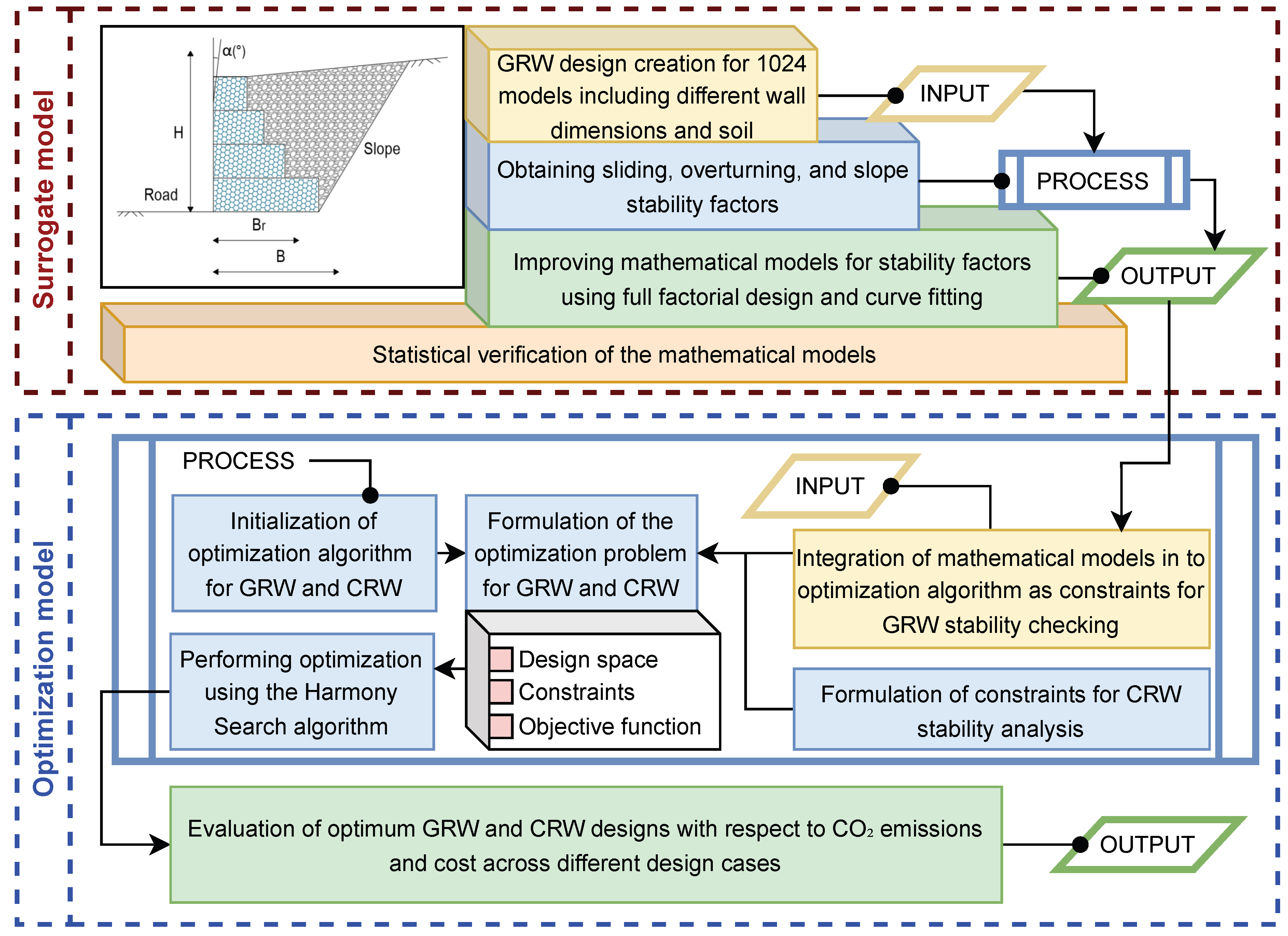
Specifically, the developed FFD-SM provides fast and dependable predictions of GRW stability factors and is incorporated as a constraint in the optimization process to ensure safety while determining optimal wall configurations. This integration enables the adjustment of wall stability and dimensions within a short computational time, accommodating various size combinations to achieve the optimal design outcome. Figure 1 illustrates the research framework, the mathematical models employed, and the overall scope of the study.
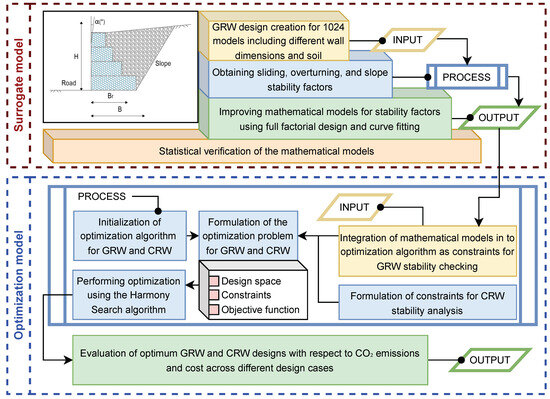
Figure 1.
Scope and motivation.
The primary motivation for this research is to develop a surrogate model that effectively manages the stability of gabion retaining walls while simultaneously addressing the trade-off between CO emissions and cost in pursuit of environmental sustainability. It is assumed that applying FFD as the statistical foundation of the surrogate model provides a robust and efficient solution, as the structured dataset generated by FFD enhances model accuracy and supports more reliable and sustainable design solutions. Specifically, this study advances the state-of-the-art by the following:
- Introducing an FFD-based SM tailored to GRWs;
- Embedding the model directly into a metaheuristic optimization framework to reduce computational effort;
- Enabling simultaneous evaluation of cost and CO emissions alongside stability criteria.
2. Definition of Problem for Surrogate Model
2.1. Gabion Retaining Wall Design
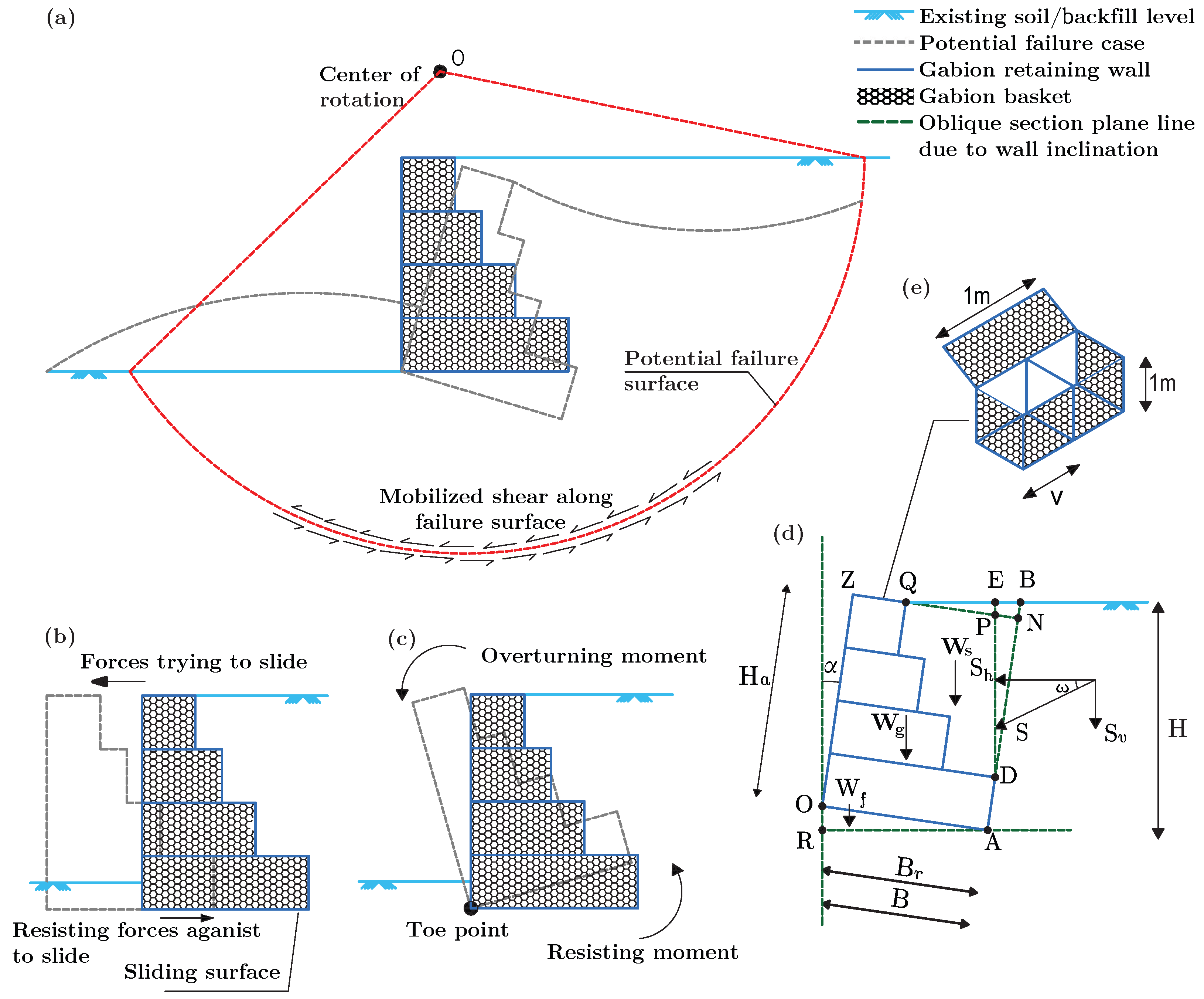
GRW construction counters lateral loads across disparate soil layers by strategically arranging and interlinking gabion baskets. This paper examines the case of slope stabilization at the roadside using GRW, including critical calculations necessary for ensuring road safety, which are provided for a unit distance of 1 m in a segment that is perpendicular to the plane of the page. Figure 2 illustrates the design parameters and loads applied to the wall for assessing the stability of the GRW.
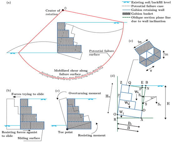
Figure 2.
Gabion retaining wall: (a) slope stability check, (b) sliding check, (c) overturning check, (d) design parameters and acting loads, (e) gabion basket detail.
The GRW design incorporates wall height (H), base width (B), gabion basket width reduction ratio (), wall inclination (), and internal friction angle () as design parameters. In Figure 2, point O represents the origin of the x–y coordinate plane. For the designated points A, O, Q, D, etc., the x and y values denote the horizontal and vertical coordinates, respectively. When the wall is constructed with an inclination, the x and y coordinates of specific points are transformed to the new coordinate system rotated by utilizing Equations (1) and (2).
The horizontal earth pressure force (S) given by Equation (3) has a critical role in the stability of the GRW. In this study, active () pressure coefficient were obtained according to Coulomb’s Theory [30] to calculate the lateral soil pressure at the effective height (Equation (5)) as in
When determining the sliding stability of the retaining wall, the safety factor of sliding, [31], which is defined as the ratio of the resisting forces against the shifting of the wall to the forces trying to slide the wall horizontally, is given by Equation (6).
The total weight (), as shown in Equation (7), is the sum of the GRW weight (), the soil weight (), and the weight of the soil between the base and the sliding surface (). and are the horizontal and vertical components of S, respectively, acting on the plane making an angle () with the horizontal. The friction angle () was taken as equal to the angle of internal friction () of backfill and base soil with the assumption that a sliding surface exists between the base and the rough face of the gabion basket.
Safety factor of overturning, [31], which is a stability criterion, is performed by using Equation (8).
In this context, , , , and , shown in Figure 2d, represent the area of the gabion wall section (m), the area of the backfill soil section (m), the area of the QEP backfill section (m), and the area of the PND backfill section (m), respectively. The variable represents the unit weight of the gabion filler contained within the gabion basket. In contrast, , denotes the unit weight of the backfill and base soil material. The resisting moments against overturning ( and ) are given by Equations (9) and (10), respectively. The horizontal component of the active soil pressure at the same point brings the gabion wall close to overturning. and are the centers of gravity of the cross-section of the gabion and the cross-section of the backfill soil, respectively.
The loads coming from the wall must be carried by the foundation, meaning that the maximum base pressure () must not be greater than the ultimate bearing capacity () of the soil. Also, the minimum base pressure, , must be greater than zero, as the soil is not able to carry the tensile stress [32]. For and , they are calculated using Equations (11) and (12).
The general bearing capacity formula proposed by Meyerhof [33] was used to calculate the ultimate bearing capacity, . The bearing capacity safety factor, , is determined by dividing this by , as in
In this study, the safety factor of slope stability, , for critical surfaces was determined using the Bishop Method [34], a slice method for slope stability analysis. To obtain , the trial-and-error method is used with any initial value given to the safety factor and selected as the failure surface. This iterative process continues until the calculated safety factor converges to the chosen safety factor. When the difference between these two values is 0.001 or less, the computed value is accepted as the safety factor. This process repeats for different failure surfaces to obtain a safety factor. The minimum slope stability safety factor is selected as the critical one among all safety factors. Since determining the safety factor for different slopes and soil parameters takes a considerable amount of time without the aid of a computer program, safety factors for slope stability are obtained using GEO5 [35], a geotechnical software that provides standard geotechnical engineering solutions.
2.2. Full Factorial Methodology and Its Mathematical Framework
Engineers and researchers optimizing complex systems may benefit from the full factorial design (FFD)-based surrogate model (SM). FFD-SM is a statistical method that enables analysis of the common effect of factors, design processes, or design parameters on the design result. In this method, experiments or designs consist of combinations of all levels of design parameters, which are selected based on the characteristics of the study. The mutual interactions affect the dependent variable, making it possible to attain an economical design. Additionally, the fact that this is a multidimensional method that investigates the linearity of functions makes it a viable option. Although the stability of a gabion retaining wall is determined using the equations mentioned above, layered gabion basket arrangements and the varying dimensions and design parameters can be challenging. Therefore, the development of FFD-SM, which determines wall stability and addresses the aforementioned issues, was employed in this study as an alternative and rapid method. Implementation details are provided in this section.
Design parameters include the wall height (H), base width (B), gabion basket width ratio (), wall inclination (), and the angle of internal friction (). The lower and upper limits of these parameters, which influence safety factors, have been set without ensuring that the stability conditions of the wall designs are met. The goal has been to analyze the effect of these parameters statistically and to improve the mathematical models for all combinations within the defined limits for wall designs. In wall design, after the first row of gabion layer, each subsequent row was reduced by the ratio from the previous row, and the gabion basket width was determined accordingly. Since the gabion baskets are assembled to a specified width in the factory, their varying width plays a crucial role in reducing wall weight and carbon dioxide emissions compared to other types of retaining walls. In developing mathematical models and investigating the effect of varying design parameter values on GRW stability, four levels have been selected for each of the five design parameters. These design parameters, along with their corresponding levels, are listed in Table 1.

Table 1.
GRW design parameters and their levels.
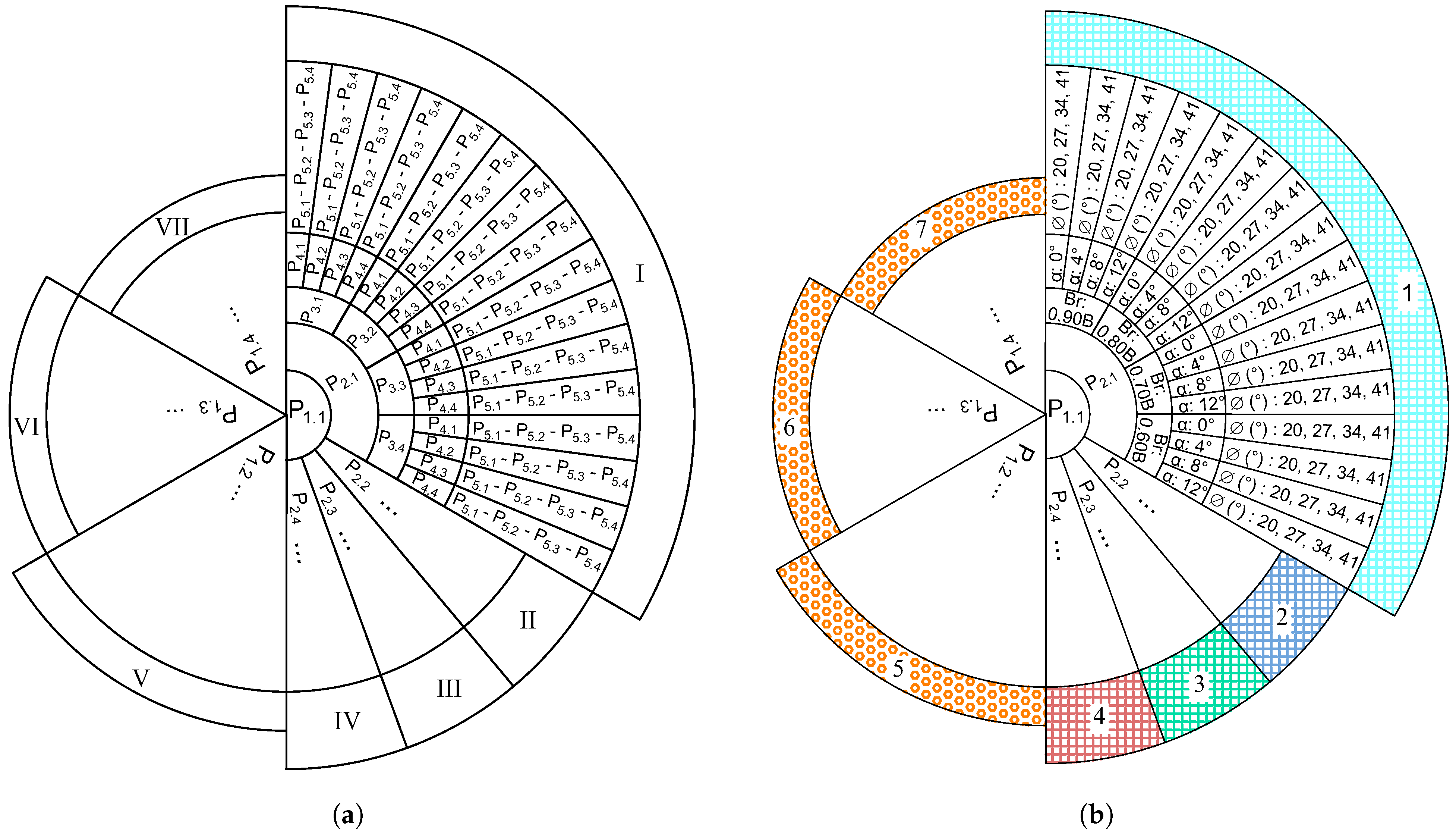
When calculating safety factors, the mathematical models have been refined using FFD, which involved 1024 () different combinations for five parameters (n) with four levels (m) each, as schematically shown in Figure 3.
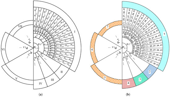
Figure 3.
Full factorial design: (a) 1024 combinations for FFD [36], (b) 1024 GRW revised designs.
In Figure 3a, (i = 1, …, n; j = 1, …, m) represents the design parameters at various levels. A specific rule was used to generate a dataset of 1024 combinations in the repeated order of parameter levels. The design parameters (n) have been established at five, with their corresponding levels (m) set at four. The initial combination consists of the first level of each parameter (, , , , and ), whereas the 1024th combination includes the last level of each parameter (, , , , and ).
Figure 3b has been recreated by taking into account the general representation of the 1024 combinations given in Figure 3a [36]. In Section 1 (turquoise color), a total of 64 distinct combinations were generated for constant value, which is a subsection of , by analyzing all possible combinations of , , and along with their respective levels. The same characteristic was applied in Section 2 (blue color), Section 3 (green color), and Section 4 (red color), each of which consists of 64 different combinations for the constant values of , , and , respectively. Thus, 256 distinct combinations were formed with the first level of the first parameter () held constant. This rule was considered in the case of Sections 5, 6, and 7 (turquoise) for , , and , respectively. Sections 5, 6, and 7 include the content of Sections 1–4, along with their respective subsections.
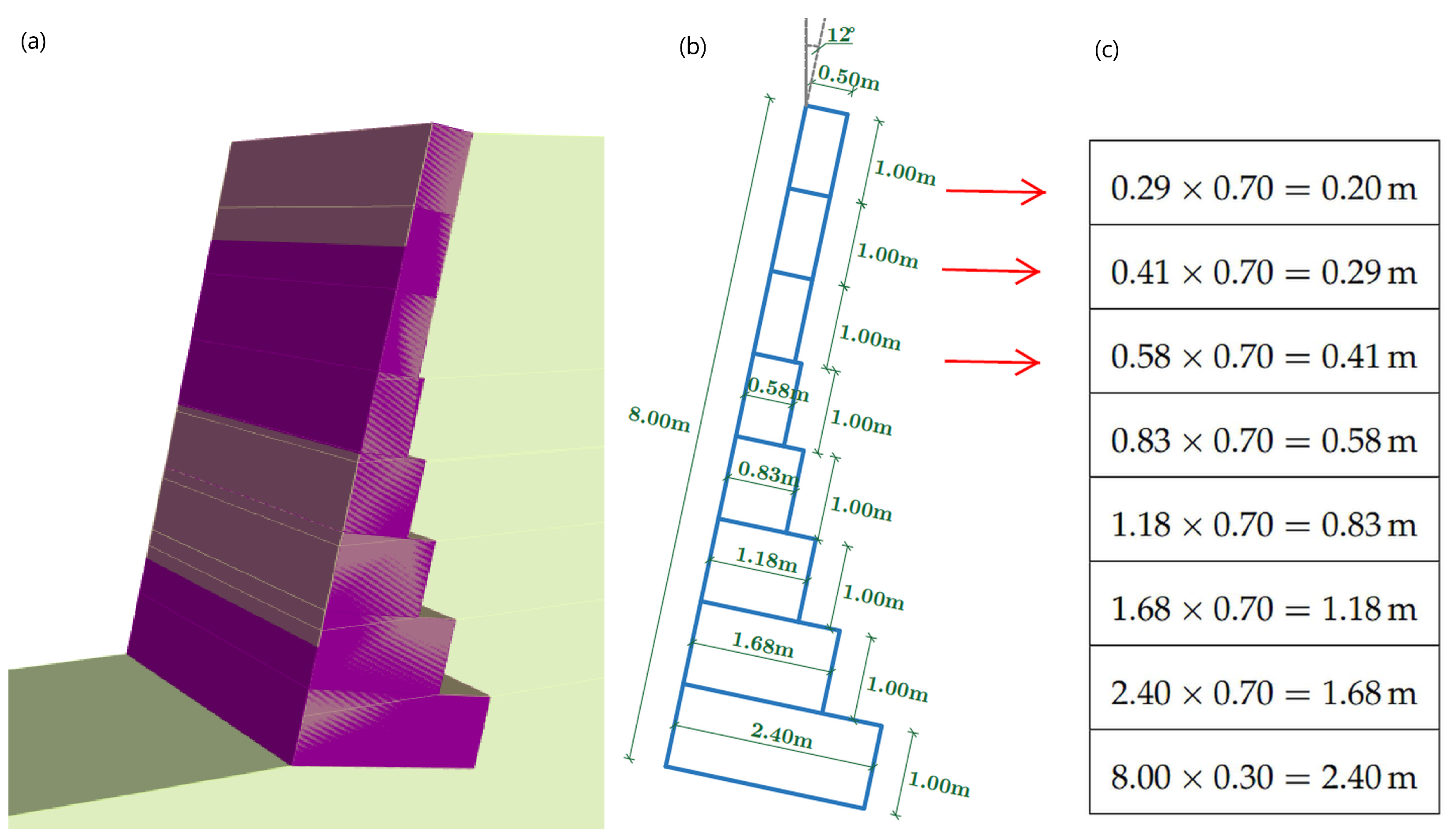
The wall designs incorporate gabion baskets with a height of 1.0 m, while the width of each row has been reduced by the gabion basket width reduction ratio (). If the width of the obtained gabion basket is less than 0.50 m, it is considered to be 0.50 m. Figure 4 presents an example wall design utilizing the GEO5 model, characterized by the parameters H = 8 m, , , , and .
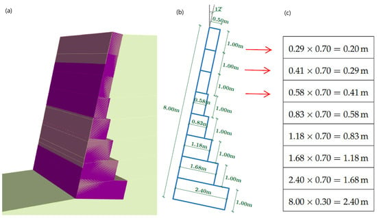
Figure 4.
Adjusting the gabion basket width: (a) GEO5 GRW model [35], (b) dimensions of gabion basket, (c) adjustment of width.
Safety factors for sliding (), overturning (), and slope stability (), required for generating stability surrogate model, were calculated for 1024 GRW designs (Figure 3) using the equations and methods outlined in the gabion retaining wall design section. In these designs, parameter values presented in Table 2 were considered for the analytical and numerical analysis of GRW.

Table 2.
Values of parameters for numerical and analytical analysis.
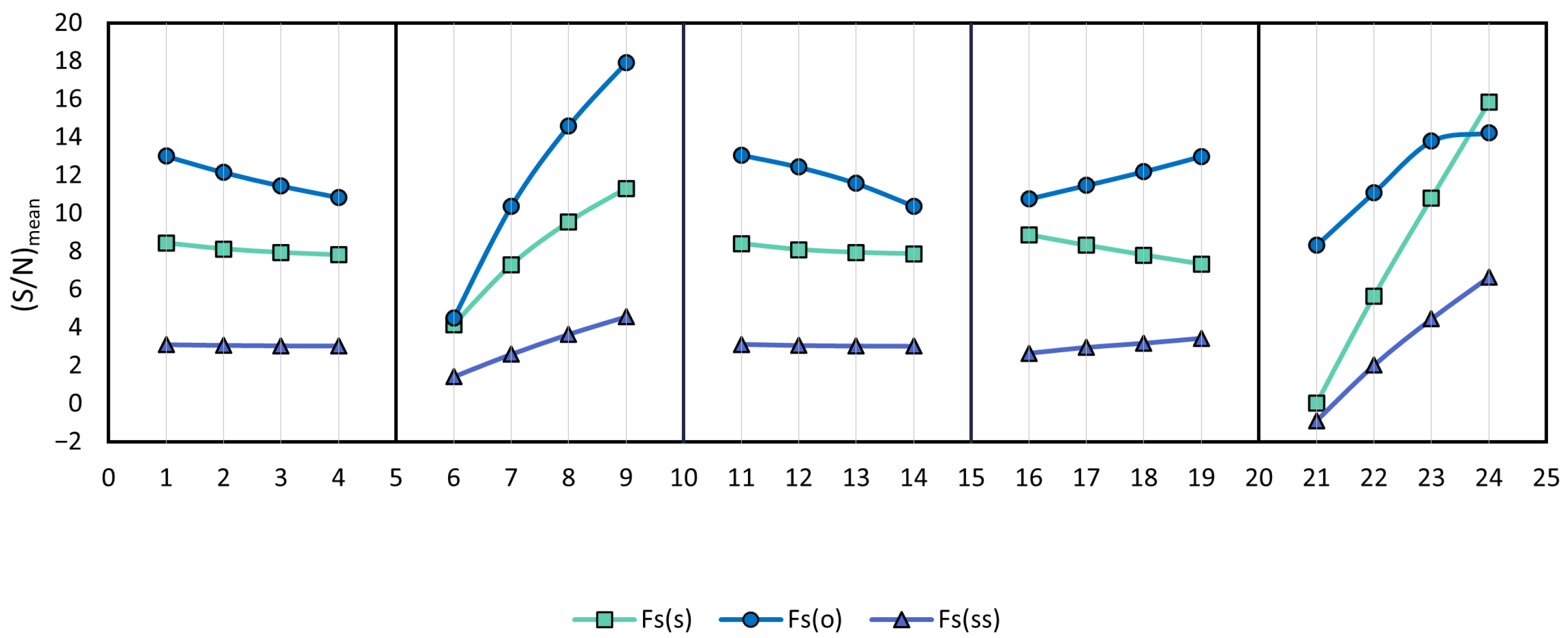
Taguchi’s signal-to-noise () ratio was employed in constructing the stability surrogate model for all , , and safety factors in 1024 GRW designs using the FFD approach. The use of ratios assesses the impact of trials and uncontrolled factors on the obtained results. This technique enhances comprehension of the relationship between input variables and output performance, leading to greater efficiency in achieving the target value. is a criterion for evaluating the performance of an experimental design, and it is calculated in three ways depending on the desired goal: “the smaller, the better,” “the larger, the better,” and “the nominal, the better.” This study applies the “bigger the better” condition, as expressed by Equation (14), to derive the ratios, given that the existing literature [37,38] indicates that more effective mathematical models are associated with larger S/N ratios. Here, Y represents the safety factor, and t denotes the number of trials.
The mean ratios for all calculated ratios for each level of all design parameters are determined by Equation (15).
is the sum of all ratios in the jth level of the ith parameter. represents the total number of combinations used to calculate . For example, represents the sum of the ratios determined for all combinations, which is H = 4m (), with equal to 256 (in Figure 3, Section I). After this calculation process, the obtained mean signal-to-noise ratios for the safety factors , , and across all parameters and levels are presented in Figure 5.
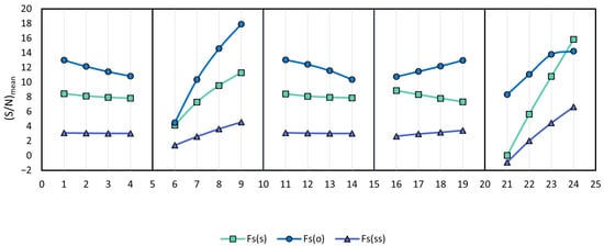
Figure 5.
Change between mean S/N ratios and levels of design parameters.
The graph shows that the base width (B) is the most effective parameter in the wall’s overturning stability. At the same time, the internal friction angle () is the most effective parameter in the wall’s sliding and overturning safety factor.
2.3. Derivation of Mathematical Models for GRW Stability
This section presents the mathematical models based on FFD-SM developed for evaluating GRW stability, together with their validation through comparative and analytical methods. The stability of GRW includes sliding (), overturning (), and slope stability () safety factors. Equation (16) formulates the general mathematical structure of safety factor models, whose content will be identified using the statistical curve-fitting technique.
Here, is defined as the total effect coefficient and is determined via Equation (17) for each safety factor, separately.
Here, the coefficient has corresponded to the average ratio of 1024 combinations, and it has been taken as 8.07, 11.86, and 3.05 for , , and , respectively. Each of the effect coefficient formulas was generated using regression analyses based on polynomial equations [39]. For the mathematical formulas of , , and , the parameter effect coefficients functions depend on parameters with specified ranges, and are displayed as in the following:
For the effect coefficient of the wall height (H),
For the effect coefficient of the base width (B),
For the effect coefficient of the width reduction ratio (),
For the effect coefficient of the wall angle of inclination (),
For the effect coefficient of the angle of internal friction (),
2.4. Performance Assessment of Mathematical Models Based on FFD-SM for GRW Stability
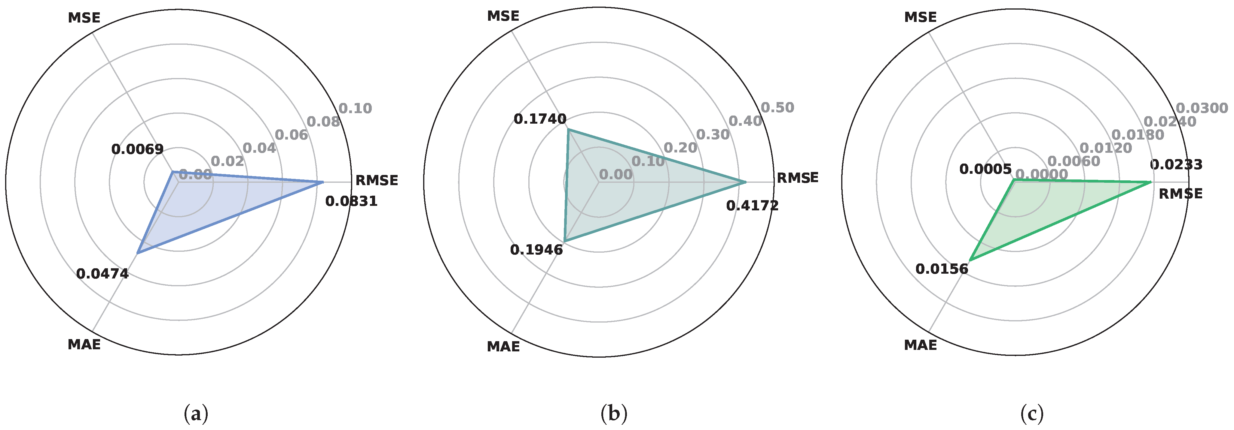
To assess the accuracy of the mathematical models, the Root Mean Squared Error (RMSE), Mean Absolute Percentage Error (MAPE), Mean Absolute Error (MAE), and Mean Squared Error (MSE) metrics, as well as the relative error () distribution, were examined using 1024 wall designs. In the given Equations (23)–(27), safety factors (, , ), obtained as the actual values from numerical analyses, and safety factors (, , ), derived from the FFD-SM models as the predicted values were considered for 1024 (n) wall designs.
MAPE values were obtained as 1.4479, 3.0352, and 1.0418 for sliding, overturning, and slope stability safety factors, respectively. While the sliding and slope stability models demonstrated reliable performance with low error rates, the overturning model exhibited slightly higher deviations. The RMSE, MAE, and MSE values shown in Figure 6 are low and acceptable, signifying commendable model performance. The minimum error rate for the sliding model (Figure 6a) was recorded at 0.007 for MSE, whereas the slope stability model (Figure 6c) achieved a metric of 0.005. The metric values derived from the overturning model (Figure 6b) demonstrate that its performance is inferior to that of the other models.
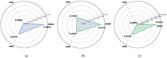
Figure 6.
Evaluation metrics: (a) Sliding. (b) Overturning. (c) Slope stability.
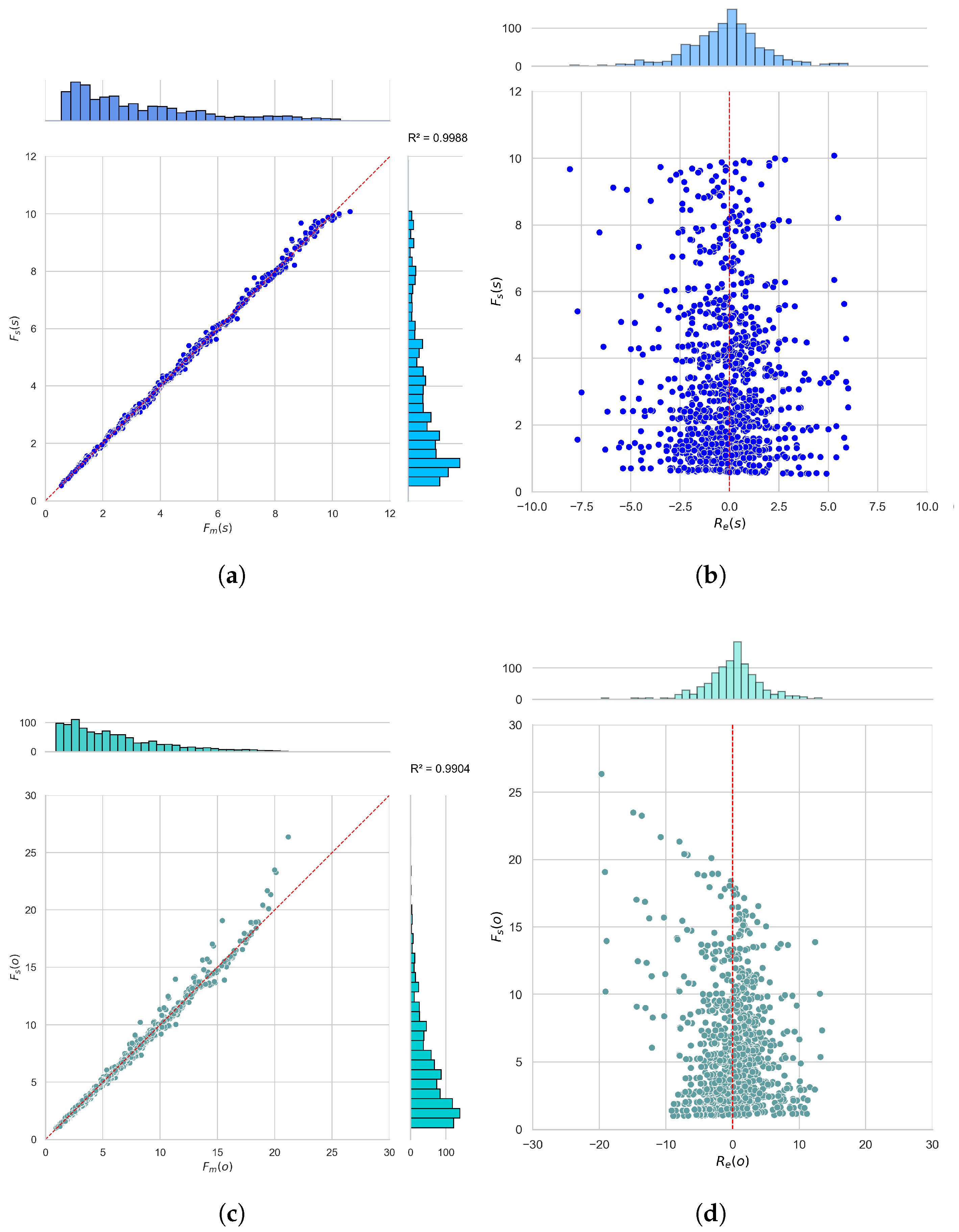
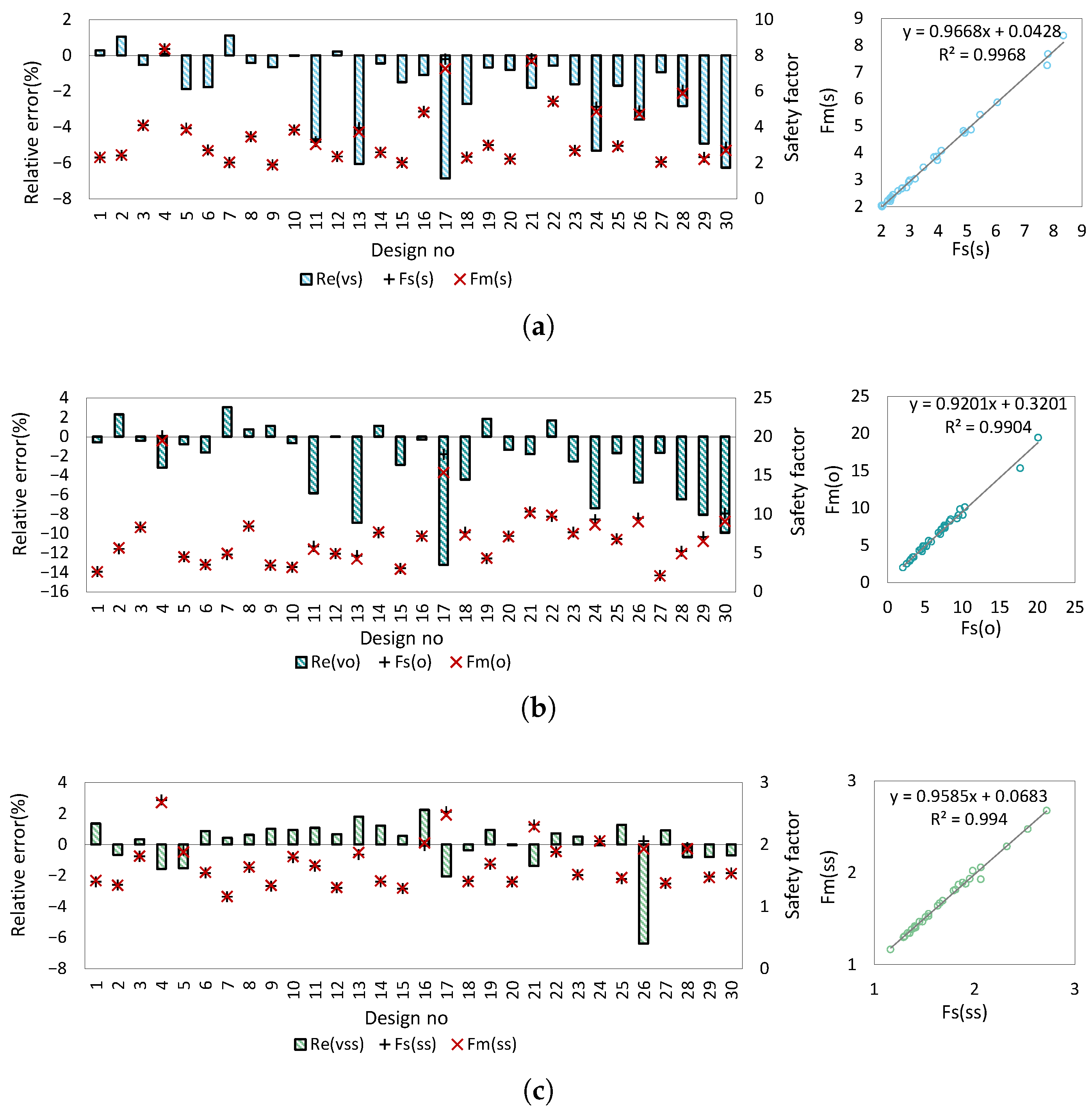
Figure 7 also displays the histograms of relative errors (), along with their distribution and the values of and . Figure 7b,d,f provide insight into the distribution of , illustrating the relationship between the actual safety factor () and with dots and a vertical reference line (). The relative positions of the dots in relation to the red dashed line highlight deviations and the accuracy of the modeled results. The Q-Q Plots (Quantile-Quantile Plots) for the and values in Figure 7a,c,e show how the intersection points of and are spread along a linear regression line, which is a dashed red reference line. In these figures, each dot indicates a paired observation comparing the modeled safety factor () and the actual safety factor (). The alignment of dots along the diagonal shows how closely the two values match. This diagonal red line represents the 1:1 correspondence ( = ). It serves as an ideal reference; the nearer the dots are to this line, the stronger the agreement between model predictions and actual values.

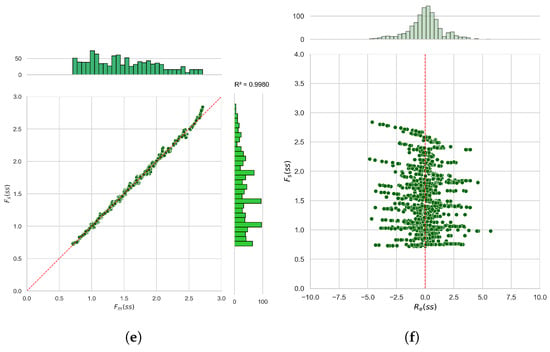
Figure 7.
Q-Q plots of and : (a) Sliding. (b) Overturning. (c) Slope stability. Histograms of : (d) Sliding. (e) Overturning. (f) Slope stability.
The distribution of most relative errors for the mathematical models is centered around zero, and the histograms of approximately display a bell-shaped pattern. The determination coefficients () for the , , and models are 0.9988, 0.9904, and 0.9980, respectively, indicating values close to 1. This evaluation suggests that the models effectively explain the variance of the dependent variable and are reliable. The results indicate that the estimates generated by the mathematical models closely match the actual values, except for the overturning safety factors, which show minor differences. Analysis of the models through relative errors reveals that the most significant errors occur in the overturning safety factor, especially when exceeds 10.
It is observed that the absolute value of the relative error (), which exceeds ±5%, is 2% of 1024 data points for , while this value is zero for . For the sliding and slope stability safety factor, the maximum absolute relative errors for 1024 combinations are less than 10% and 5%, respectively.
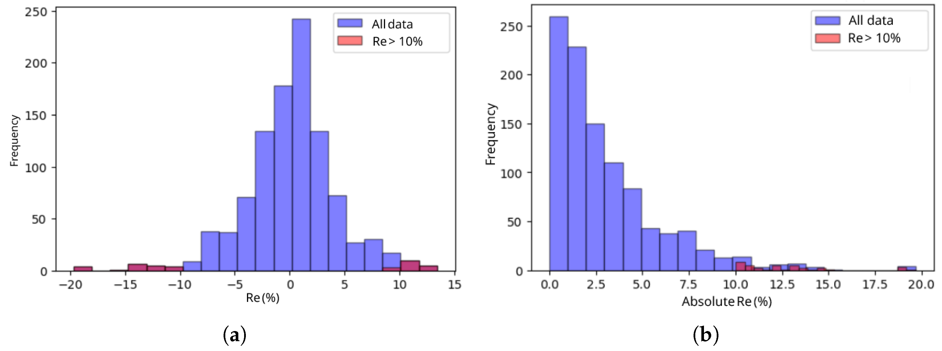
As demonstrated in Figure 8, the distribution of indicates that the error associated with exceeds (+10) and falls below (−10), occurring in 38 out of 1024 wall design configurations. This value constitutes approximately 4% of all evaluated design configurations during the model development process. These cases concentrate at geometric extremes; higher wall inclination ( = 12°) together with limiting base–width ratios (e.g., = 0.30 with H = 10 m) and reduced basket widths, = 0.80–0.90B). Similarly, for H = 4 m, combinations with B=0.75–0.60 H, = 0.80–0.90B), and = 12° tend to push the active earth–pressure resultant to longer lever arms and shift the base resultant toward the toe, increasing the sensitivity of the moment ratio.
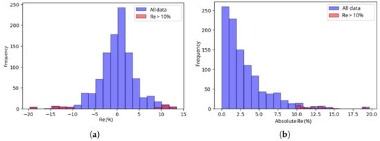
Figure 8.
Distribution of relative error in all data. (a) . (b) Absolute .
As defined in Equation (8), the overturning safety factor is obtained by dividing the resisting moment () by the overturning moment (). In retaining wall design, both and are calculated by multiplying the loads acting on the wall with their respective lever arms measured from the toe point. The lever arm (x), determined by load location and geometric parameters such as base width (B) and wall inclination, is highly sensitive and strongly influences moment equilibrium. Even small geometric variations can therefore disproportionately amplify deviations in [40,41]. The eccentricity of the resultant load (e) relative to the base also plays a crucial role in overturning behavior. When , tensile stresses at the heel do not occur, and toppling is prevented. Conversely, when this condition is not satisfied, as observed in cases with absolute relative errors greater than 10%, the imbalance between and increases and leads to larger deviations in predicted overturning factors of safety. Parametric and probabilistic studies support this interpretation, indicating that overturning exhibits greater sensitivity and uncertainty than sliding when geometric or loading conditions vary [42]. By contrast, the surrogate models developed for sliding and slope stability, based on the same dataset, yielded consistently lower errors, further confirming that the higher overturning error arises from the inherent mechanism of moment equilibrium rather than from deficiencies in the surrogate modeling framework. This behavior is consistent with the speed–accuracy trade-offs widely acknowledged in surrogate modeling approaches. This situation suggests that the elevated error in the overturning factor of safety primarily stems from geometric sensitivity, indicating an interaction between the surrogate model and the physical mechanism rather than a systematic deficiency in the approximation. Furthermore, the speed of the surrogate model’s advantage renders a certain margin of error permissible for its intended application. It has been extensively emphasized in the literature that analogous modeling techniques in geotechnical engineering and broader engineering optimization contexts accept a minor compromise in accuracy in exchange for increased speed and computational efficiency [43,44]. In this regard, our proposed approach is both methodologically consistent with existing approaches in the literature and provides a practical and dependable alternative for engineering applications.
Model accuracy is assessed by excluding the 1024 GRW combinations in Figure 3, with randomly selected new design parameters presented in Table 3. The design parameters, which fall within the specified lower and upper limits for established mathematical models, are taken into account, excluding any parameter levels listed in Table 1. For instance, the wall design characterized by parameters H = 4 m, B = 0.30H, = 0.90B, = 8°, and = 34° is not included in the 1024 combinations.

Table 3.
Design parameters for verification analysis.
Utilizing the safety factors (, and ) as per the wall designs in Table 3, Figure 9 presents plots of relative errors and Q-Q plots. Histograms of safety factors show that the highest absolute relative error for the safety factors of sliding, overturning, and slope stability is 7% (Figure 9a), 13% (Figure 9b), and 6% (Figure 9c), respectively. It can be safely stated that mathematical models of safety factors for sliding and slope stability can be used to determine the stability of a wall with a relative error of 10%. It is suggested to use mathematical models for the safety factor of overturning with a 20% relative error. Negative relative errors are commonly observed because the safety factors calculated from mathematical models tend to be greater than those derived from numerical analyses, as shown in Figure 9. This outcome indicates that the design is safe, since the safety factors from the mathematical models of GRW do not exceed the actual stability conditions.

Figure 9.
Relative error plot and Q-Q plots for GRW design validation: (a) Sliding. (b) Overturning. (c) Slope stability.
The FFD-SM models are capable of effectively evaluating the stability of the GRW under real-world conditions in a prompt manner. The surrogate model, which employs a fully factorial design with an established acceptable error rate, has been utilized to assess the stability of the complex-designed GRW. It has been confirmed to be an efficient and reliable instrument within a short period of time. This efficiency not only simplifies the evaluation process but also improves the accuracy of stability assessments. Consequently, researchers and engineers can make better-informed decisions, leading to improved safety and performance across various applications. This capability enables more efficient decision-making, ultimately leading to improved resource management and enhanced stability in dynamic environments. To facilitate the utilization of the mathematical models developed for controlling GRW stability with FFD-SM and to enhance their accessibility for all users, a Jupyter notebook file of this model is provided as Supplementary Material.
3. Definition of the Optimization Problem: Cost and Emission Trade-Off in Retaining Wall Designs
3.1. Metaheuristic Optimization Algorithm
The Harmony Search Algorithm (HSA) was employed as the metaheuristic optimization algorithm to investigate the optimum designs of the cantilever retaining wall (CRW) and the gabion retaining wall (GRW). Geem et al. [45] developed HSA, a heuristic optimization method inspired by the collaborative process of musicians in creating effective music. HSA is superior to other heuristic approaches in that it is simple to use, can produce results in a relatively short amount of time despite numerous iterations, can handle both continuous and discrete variables, and can determine global solutions during optimization. HSA is widely utilized in various fields, as it excels at solving design optimization challenges and identifying optimal solutions. These include civil, electrical, industrial, software, and mechanical engineering. Other topics include scheduling, clustering, networking, image processing, and more [46].
In the present study, the design variables optimized by HSA include the wall base width, stem thickness, heel length, and toe length for the CRW, as well as the gabion basket dimensions for the GRW. The objective function was formulated to minimize the total construction cost, while surrogate constraints representing stability requirements (e.g., factors of safety against sliding and overturning, and slope stability limitations for GRW) were imposed to ensure structural safety. These surrogate constraints act as engineering-based approximations that guide the optimization process toward feasible and practical solutions.
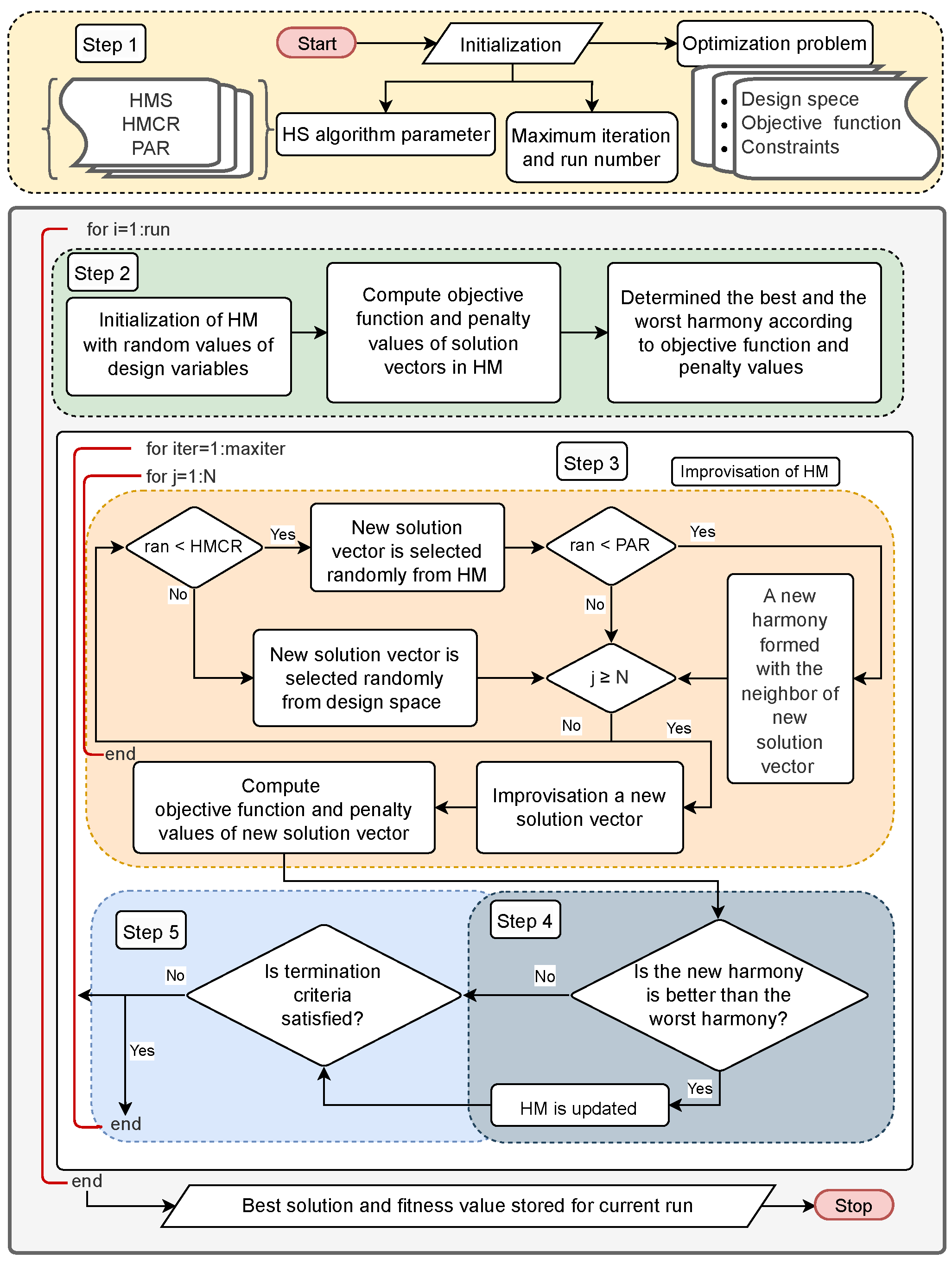
The steps for implementing HSA, whose flowchart is given in Figure 10, are listed below:
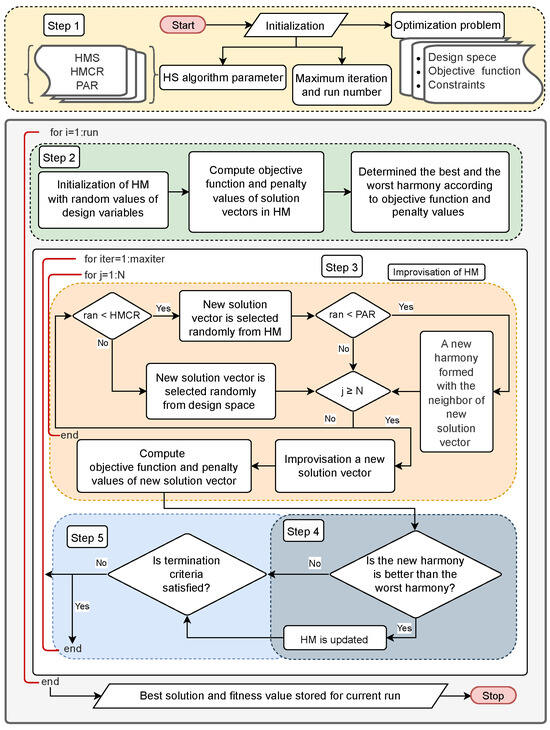
Figure 10.
Harmony search algorithm flowchart.
Step 1—Parameter initialization and design space creation: Set up the parameters and create the design space. The values for HSA and the range for each design variable are defined. A design space is formed using these ranges. Next, some critical HSA parameters are configured, such as Harmony Memory Size (HMS), Harmony Memory Considering Rate (HMCR), Pitch Adjusting Rate (PAR), and the maximum number of Iterations (MaxIter). Then, the run is executed. HMS is the number of solution vectors (rows) in the harmony memory (HM). HMCR determines which values are selected from the HM, and PAR controls how those values are fine-tuned.
Step 2—Harmony memory initialization: To start the harmony memory (HM) matrix, values are chosen at random from the design space. Each row in the matrix represents a possible solution vector for the corresponding design parameter. The matrix has N columns, equal to the number of design variables. HM has values, where i is the ith possible solution (i = 1, 2, …, HMS) and j is the jth design variable (j = 1, 2, …, N). These steps form the basis of HSA, which enables us to quickly identify the best solutions to a wide range of optimization problems.
Step 3—Enhancement of the harmony memory matrix: The harmony matrix is enhanced in this step. In the HSA, the development of a new solution vector is governed by the HMCR and the PAR. A new solution vector is created during the selection process by selecting values from the current HM with an HMCR probability. The design variables for the new solution vector are randomly chosen from the design space with a chance of (1-HMCR) if they are not selected from HM. When choosing a design parameter from HM with PAR possibility, it is examined to determine whether it can be altered by substituting its lower or upper neighbor, contingent on PAR. The process of fine-tuning enhances the solution’s ability to discover new ones.
Step 4—Updating the harmony memory matrix: After obtaining a new solution vector, the values of the objective function and penalty are found for that vector. The new solution replaces the worst one if this value is better than the worst in the HM. Deb’s rule is taken into account in determining the best and worst solutions. Deb’s rules [47], a standard method for handling constraints in optimization, were used as the constraint-handling approach to ensure the stability of retaining walls. Deb’s rules provide that the algorithm considers infeasible solutions that could lead to feasible regions in later iterations by favoring those with fewer constraint violations (penalty). At each iteration, Deb’s rules guided the evaluation of surrogate constraints by penalizing or rejecting infeasible solutions while prioritizing those that violated fewer stability requirements. When both solutions are feasible, the one with the higher fitness value is selected. For example, a design with a factor of safety against sliding slightly below the allowable limit was retained over one that failed multiple stability checks, thereby allowing the search process to approach feasible regions gradually. This mechanism ensured that cost and CO minimization were not achieved at the expense of geotechnical safety.
Step 5—Termination of the algorithm: The HSA concludes upon reaching the maximum number of iterations, designated as MaxIter. Steps 3 and 4 are iteratively repeated to enhance the HM.
Contemporary optimization strategies, such as Deb’s rule, merit greater attention due to their flexibility and ability to integrate with established optimization frameworks [48]. Additionally, the HSA parameters were set to HMS = 20, HMCR = 0.90, and PAR = 0.35, consistent with findings from other studies [36,45] and supported by preliminary sensitivity analyses. These analyses confirmed that the chosen values provide an effective balance between exploring the design space and exploiting promising solutions for the current retaining wall optimization problem.
3.2. Mathematical Problem Definition and Optimization Framework for Cantilever and Gabion Retaining Walls
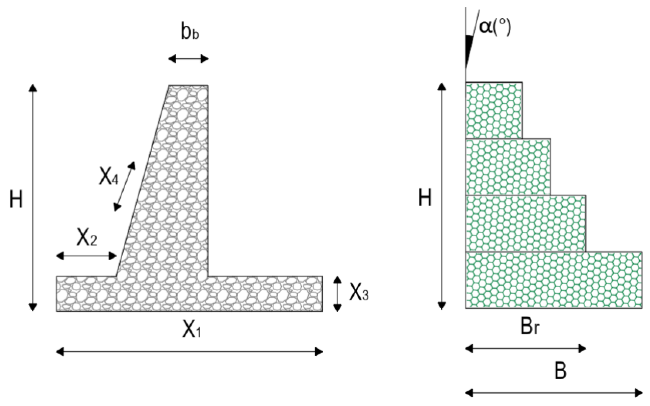
In this section, the definitions of the cantilever retaining wall (CRW) and the gabion retaining wall (GRW) optimization problems are explained. The optimization problem was addressed to derive the minimum wall costs, , and (CO2) values for the GRW and the CRW under various wall design cases, and to analyze the relationship between them. When looking at the GRW and the CRW for optimization, the wall’s geometry limits, which were based on its size and its stability, which included sliding, overturning, slope stability, and bearing capacity safety factors, were all taken into account as constraints [49]. Optimum wall designs were evaluated to ensure safety against sliding, overturning, bearing capacity, and slope stability, with allowable safety factors of 1.5, 1.5, 3.0, and 1.5, respectively [32]. In the optimization problem for GRW and CRW, wall dimensions were used as the discrete design variables, with intervals () between the lower and upper bounds. The optimization problem was defined by discrete design variables given in Figure 11: for CRW, the base width (), toe extension (), base thickness (), and front wall face inclination () are considered, while for GRW, the base width (B), the width reduction ratio of the gabion basket (), and the wall inclination () are taken into account.
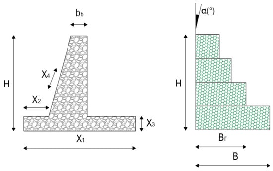
Figure 11.
Design variables of CRW and GRW, respectively.
The GRW optimization problem is defined by Equation (28).
For sliding (), overturning (), and slope stability () safety factors checking of the GRW, statistically generated mathematical models, which are detailed in Equations (16)–(22), were utilized in the optimization analyses.
The CRW optimization problem is defined by Equation (29).
The research conducted by Uray et al. [50] served as the basis for the design variables and constraints used to evaluate the stability of the CRW design. Safety factors such as sliding (), overturning (), and bearing capacity () from the mentioned study are used to define the optimization problem for CRW stability. In addition, the mathematical model from the literature, which had been statistically improved, was considered for the safety factor related to slope stability () in CRW [38].
The scenario was considered to determine which wall would be more economical and environmentally friendly when the slope is supported with CRW or GRW, ensuring the safety of an operational road located at the edge of a natural slope. In this scenario, the existing slope mass with a 5% slope () is initially excavated, and the wall is then constructed. After the wall construction, backfilling with a 2% slope () is conducted to the space between the back of the wall and the excavated slope. Figure 12 presents the scenario for constructing GRW or CRW along with the design variables.

Figure 12.
Considered scenario and design variables for optimization problem of CRW and GRW, respectively.
Equation (30) for and Equation (31) for (CO2) represent the mathematical expressions for the objective functions of the CRW and GRW optimal designs. These functions help identify the most efficient designs by balancing economic and environmental impacts, emphasizing the importance of customizing wall designs to specific site conditions.
CRW stands for six construction activities (), which are the construction items (): the amount of earth that needs to be removed (in cubic meters), the area of the foundation formwork and stem (in square meters), the amount of used concrete (HA-30) for the foundation and stem (in cubic meters), and the amount of soil that needs to be backfilled (in cubic meters). GRW has three construction activities (), which are the construction items (): the amount of earth that needs to be removed (in cubic meters), the amount of gabion wall (in cubic meters), and the amount of backfilled soil (in cubic meters). The unit cost and CO emission coefficients for each amount of construction item (), which correspond to the amount of work in square meters or cubic meters, are and , respectively. These numbers come from studies in the literature [13,15,51]. CRW and GRW for unit construction works, including details such as cost and CO emission coefficients, are tabulated in Table 4.

Table 4.
Unit values of construction items for CRW and GRW.
Optimization analyses were conducted to compare the most effective CRW and GRW designs for various cases, based on cost and CO2 emissions. Eighteen design cases for each wall type were examined, considering three different wall heights (4, 6, and 8 m), three types of base soils (D, C, and B local soil classes, see Table 5), and two objective functions.

Table 5.
Soil properties for different classes and backfill.
To ensure a consistent comparison between the optimization results of GRW and CRW, optimization analyses were conducted using identical design parameters. The soil properties (Table 5), wall height (4 m, 6 m, 8 m), and base width (0.25 H–1.0 H)—critical factors for wall stability—were kept constant for both retaining wall types. Since the wall height and soil conditions were identical, the loads acting on both walls were comparable, allowing for the observation of variations exclusively from the geometric differences between GRW and CRW. The comparative analyses, therefore, focused on assessing how these geometric variations influence cost and emissions.
4. Results and Interpretations from Surrogate Model-Driven Design Optimization
4.1. Optimization Analyses
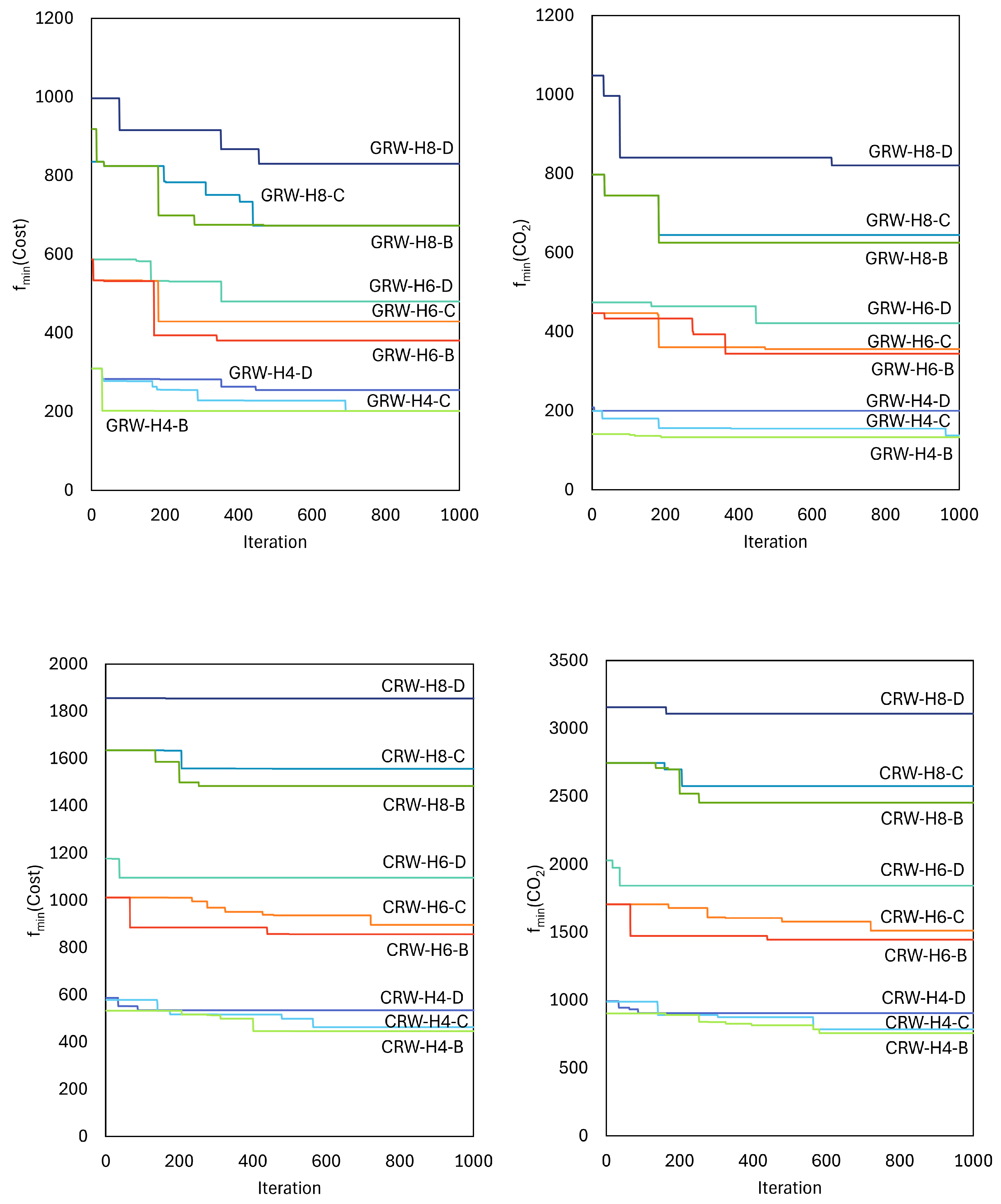
This section presents the optimal CRW and GRW designs for the cases of H4-D, H6-D, H8-D, H4-C, H6-C, H8-C, H4-B, H6-B, and H8-B based on two objective functions. In optimization analyses, the best designs for CRW and GRW were identified separately for the and CO objective functions. Then, it was examined how the optimal values varied across different design cases. For this, the Harmony Search Algorithm (HSA) was run 500 times using the techniques described in the previous sections, with a maximum of 10,000 iterations per run. The iteration history plots for 1000 iterations aimed at finding the optimal values of and CO functions are shown in Figure 13.
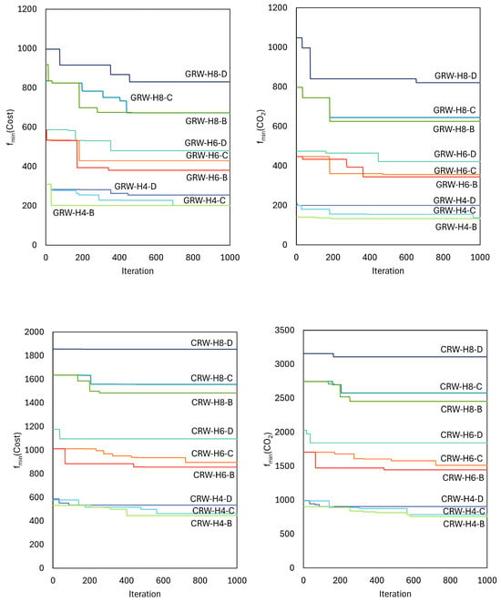
Figure 13.
Iteration history graphs of cost and CO emission values for GRW and CRW.
To examine the algorithm’s sensitivity and stability with respect to initial conditions, multiple independent runs were performed for each design case. Specifically, the HSA was executed 500 times, each run consisting of 10,000 iterations. The mean, median, and standard deviation (Std. Dev.) values reported in Table 6 and Table 7 indicate that the optimal solution values are consistently very close to the mean [52]. This evaluation demonstrates that the algorithm consistently and reliably provides results even under varying initial conditions and across diverse design scenarios. The generally low standard deviation further corroborates the stability of the results and suggests a low probability of entrapment in local minima [53].

Table 6.
Statistical values for all runs of cost objective function (, €/m).

Table 7.
Statistical values for all runs of CO emission objective function (CO, kg/m).
Additionally, the proximity of the mean and median values indicates a symmetric and reliable solution distribution [54]. Although iteration-wise convergence curves cannot be directly presented due to the absence of recorded iteration histories, the statistical distributions observed in this study align with the typical convergence behavior of HSA reported in the literature. Previous studies have thoroughly established that HSA converges monotonically and steadily towards the global optimum [45,55,56]. The low-variance outcomes obtained in this study are therefore consistent with these established findings. Regarding parameter determination, the principal HSA parameters (HMS, HMCR, PAR) were selected according to ranges frequently adopted in the literature [36,45,56]. These parameters were validated through small-scale preliminary experiments and then fixed across all problem instances, thereby ensuring stable and reliable algorithmic performance under different design scenarios.
The results further reveal that GRW designs consistently outperform CRW designs in terms of both cost efficiency and environmental impact ( and CO emission values). This result confirms that GRW configurations constitute not only more cost-effective but also more environmentally sustainable alternatives. Consequently, the proposed HSA methodology supports sustainable decision-making in design while simultaneously ensuring robust optimization performance.
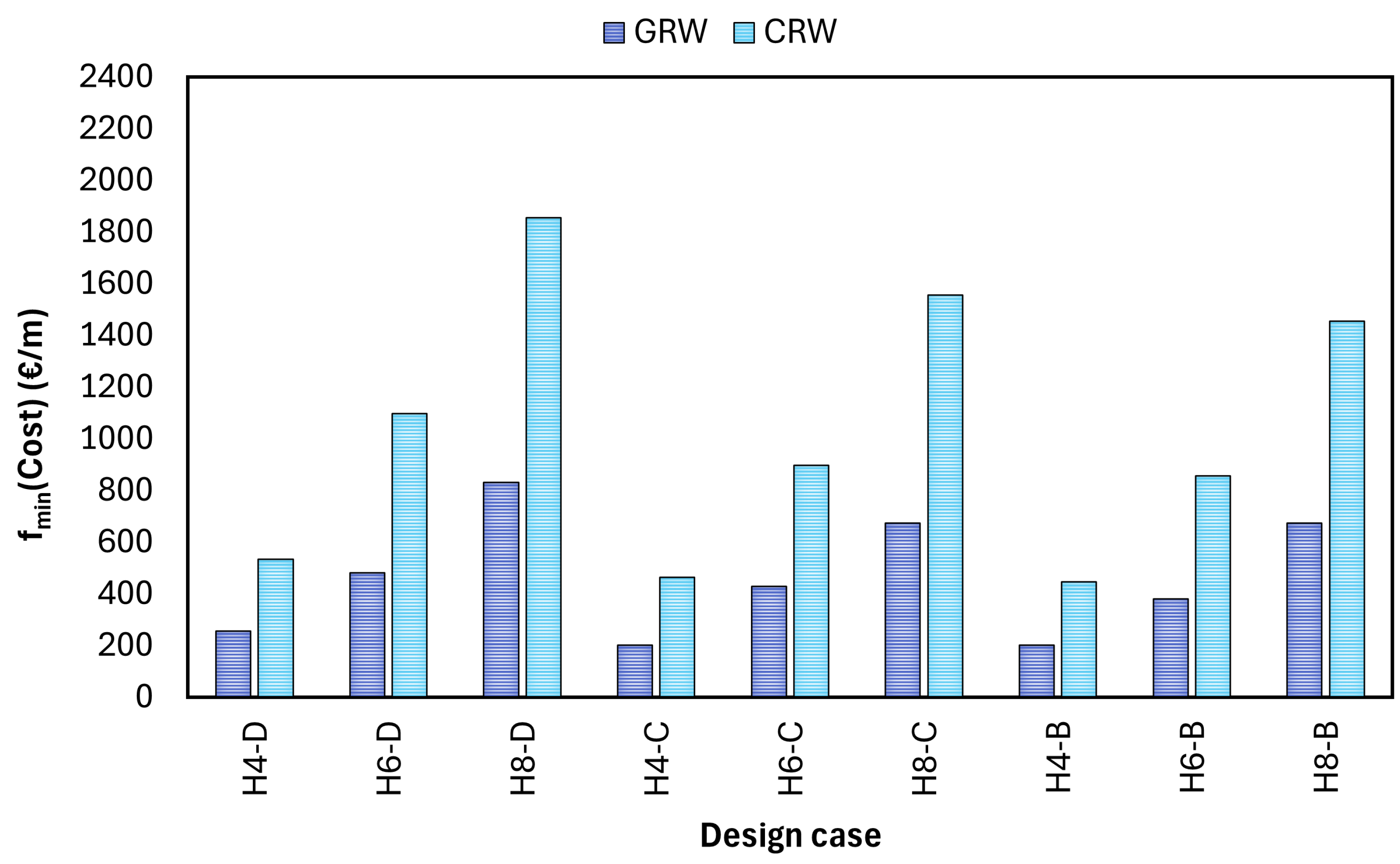
As shown in Figure 14 and Figure 15 for the optimal cost () and emission (CO) values, respectively, raising the wall height in the same soil type for both CRW and GRW optimal designs leads to higher costs and CO emissions. To maintain stability, the wall’s dimensions increase proportionally with its height, as lateral loads become greater with rising soil pressure. Additionally, it is observed that the increase in objective function values occurs because the soil quality degrades from B-type (good) to D-type (poor). When a retaining wall of the same height is built in different types of soil, the cost and CO emissions typically decrease as the soil becomes stronger or better. When a retaining wall of identical height is constructed on soils exhibiting higher strength, both the bearing capacity and shear strength of the soil are enhanced. From a theoretical perspective, soils with a greater internal friction angle exert a decreased active horizontal pressure force on the wall, as the coefficient of active earth pressure () is diminished. This reduction in lateral soil load directly contributes to improved wall stability, facilitating the design of smaller wall sections and thereby decreasing the consumption of construction materials.

Figure 14.
Comparative values for CRW and GRW optimum designs.
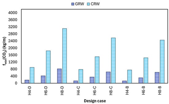
Figure 15.
Comparative CO values for CRW and GRW optimum designs.
It is seen that when a retaining wall of the same height is built in different types of soil, the cost and CO emissions typically decrease as the soil becomes stronger or better. Supporting this theoretical rationale, Shamsabadi [57] conducted an analysis of the horizontal earth pressure coefficient () across various soil properties utilizing the log-spiral-Rankine limit equilibrium model, Shields–Tolunay, Rankine, Coulomb, Mononobe–Okabe, Mylonakis et al., and Trial Wedge methodologies. Their findings demonstrated that the variation in Ke concerning soil strength parameters, notably the internal friction angle, significantly impacts wall design criteria. Specifically, soils with elevated friction angles exhibited diminished lateral pressure requirements, resulting in more efficient structural solutions. Kowalska and Jastrzębska [58] conducted triaxial tests indicating that weak cohesive soils, characterized by undrained shear strengths below a certain threshold, do not perform adequately under loading conditions, thereby yielding lower bearing shear capacities. Li et al. [59] discussed the influence of spatial variability in buried footings on bearing capacity, noting that a lack of uniform shear strength often characterizes weaker soils, consequently reducing their carrying capacity. The inconsistency of shear paths in such soils can considerably diminish the overall load-bearing potential of a foundation, as varied shear paths may lead to differing shear strengths under stress.
Within the scope of this investigation, these theoretical and analytical insights are reflected in the observation that walls constructed within stronger soil environments can be designed with smaller dimensions while still maintaining stability. Consequently, such designs inherently require less material, resulting in lower CO2 emissions and reduced construction costs. This outcome aligns with findings documented in the literature [50,60], reinforcing the conclusion that constructing retaining walls of equal height in different soil conditions highlights the sustainability and economic advantages of using stronger soils.
When comparing gabion retaining walls (GRWs) to concrete retaining walls (CRWs), it is clear that GRWs consistently outperform CRWs in terms of both cost and environmental impact. Building a CRW retaining wall instead of a GRW to support horizontal soil pressure between two different ground levels costs, on average, 55% more across all design scenarios. This increase is about 78% in terms of CO emissions. The case study analysis further illustrates this trend. The designs examined demonstrated that H4-B had the lowest cost and CO emissions, whereas H8-D, which had weak soil and a taller wall, had the highest. This variation is rooted in how engineers actually work, where stability requirements make materials more expensive in less stable soil conditions. This outcome, which closely reflects reality, results from efforts to meet the wall’s stability standards. Importantly, GRWs had a clear advantage over CRWs even in the most challenging situations. This result suggests that the greater sustainability of GRWs is not limited to specific cases but is evident across all design scenarios.
Figure 16 shows that the wall dimensions of CRW are generally consistent in terms of cost and CO emissions goals. This outcome demonstrates that the CRW design, which incurs the lowest price, also generates the minimal quantity of CO, rendering it both cost-effective and ecologically sustainable for the chosen design scenario. The safety factors identified for the best CRW indicate that the walls will remain stable. The safety factor for bearing capacity is exceptionally high for the D-type soil environment and all wall heights in the design case. In these designs, where the ratio of the base width to the wall height () is about 0.90, significantly increasing the foundation size increases the safety factor for bearing capacity. The ratio of the foundation width to the wall height () was about 0.60 for all wall heights in the B soil class. For all design cases, the increase ratio for toe extension, calculated as the ratio of the height of the wall to the width of the base, was 0.60 (). The ratio of base thickness to wall height (()) was 0.06 for walls 4 m and 6 m high and about 0.075 for walls 8 m high. This ratio gets bigger as the wall gets taller. The result shows that taller walls require greater stability. Since the wall’s thickness or depth remains relatively constant, regardless of height, these values () remain relatively low at all wall heights. This kind of result could mean that the designer chose to keep the materials efficient while making sure the structure remained strong. Setting the parameter to zero in all design cases aligns with the findings of other researchers, who have found that it does not improve wall stability [61].
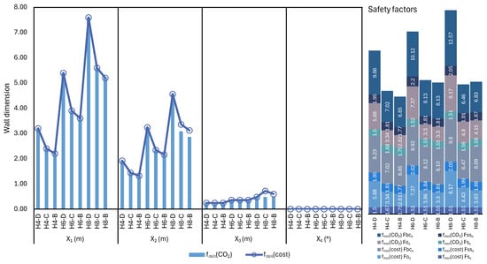
Figure 16.
Optimum wall dimensions with safety factors for CRW.
Figure 17 clearly shows how wall sizes change with height when costs and CO emissions values were obtained as a minimum. The best results from the GRW design indicate that the walls are mostly the same size compared to CO and . Only minor differences appear in the width reduction ratio of the gabion baskets (), which is approximately 0.50. As explained earlier, when building a gabion retaining wall by stacking gabion baskets, the width of each basket is determined by multiplying the previous row’s basket width by . Lower building costs and emissions are achieved with a GRW that has narrower widths in each row compared to its predecessor. Since all safety factors exceed the limit, maintaining the wall’s stability is aided by modifying . Due to the increased height requirement for sliding and overturning safety regulations, the base width (B) increases substantially as the wall height rises from 4 m to 8 m. All design cases have a constant inclination angle () of 12, which improves stability and reduces failure risk from lateral earth pressures. The average base width of the GRW foundation was 0.45 () of the total wall height, and the safety factors for bearing capacity were lower than those for CRW.
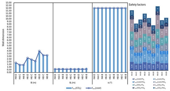
Figure 17.
Optimum wall dimensions with safety factors for GRW.
4.2. Cost–CO Balance: Findings and Implications for Practice
In this study, we solved two single-objective optimization problems separately—minimizing total cost and minimizing CO2 emissions (CO2)—for a set of retaining-wall design scenarios (varying wall heights and soil conditions). Therefore, to examine the relationship between optimum cost and CO2 emissions, the cost value (CO) was calculated based on the wall dimensions obtained for the objective function CO. This approach enabled us to interpret the cost savings of constructing the retaining wall in relation to the optimum emission value for various design scenarios. To examine the cost–emissions relationship without running a full multi-objective analysis, we re-evaluated the cost at the CO-optimal design. Formally,
Comparing the CO-optimal cost with the actual cost-optimal value,
quantifies the budget impact of prioritizing emission reductions across scenarios. The per-scenario differences are summarized with dumbbell plots in Figure 18 for GRW and Figure 19 for CRW. In these figures circles (●) represent the cost-optimum designs, while triangles (▲) represent the CO-optimum designs. Different colors correspond to the various design cases (e.g., H4-B, H6-C, H8-D, etc.). The numerical values next to the markers indicate the cost difference and percentage increase relative to the cost-optimum design.
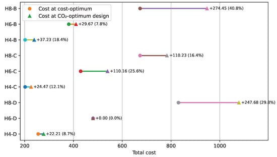
Figure 18.
Cost impact when choosing CO-optimal designs for GRW (per case).
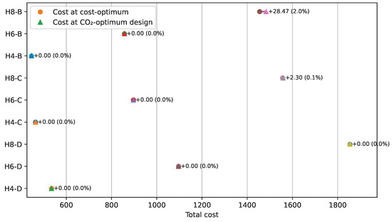
Figure 19.
Cost impact when choosing CO-optimal designs for CRW (per case).
Figure 18 shows that the cost of converting to the CO-optimal design of GRW might go up by as much as 40.78% in some circumstances (median 16.38%). The biggest jump is +274.45% (about 40.78%) for H8-B, then +247.68% (about 29.83%) for H8-D, and finally +110.16% (about 25.65%) for H6-C. H6-D has the smallest increase, which is 0%. The cost of the two most extreme solutions is the same. Figure 19 shows that switching to the CO-optimal design leads to at most a 1.96% increase in cost across scenarios (median 0%). The largest absolute change is observed for H8-B with (≈1.96%), followed by H8-C with (≈0.15%). All remaining cases exhibit , indicating identical costs for the two extreme solutions (cost-optimal vs. CO-optimal) in those configurations.
Interpreting the trade-off plots jointly, a CO2-oriented design for the cantilever retaining wall (CRW) is essentially cost-neutral or very low-cost in most scenarios, whereas the gabion retaining wall (GRW) exhibits a pronounced cost–emissions trade-off, particularly for higher walls. These observations pertain to within-system choices (i.e., GRW vs. GRW; CRW vs. CRW). In cross-system terms, however, GRW can still dominate CRW in absolute magnitudes: even when the CO2-optimal GRW entails a cost increase of up to ≈40%, its total cost can remain below that of CRW, and its absolute CO2 is typically lower as well. Consequently, when cost and emissions are the primary decision criteria, GRW is generally the preferred option. CRW remains a viable alternative where non-economic or practical considerations are paramount—such as material availability and logistics, labor and construction time, geotechnical constraints (e.g., bearing capacity, settlements), drainage, durability, maintenance burden, and expected service life.
4.3. Accuracy Performance for Surrogate Model-Driven Design Optimization
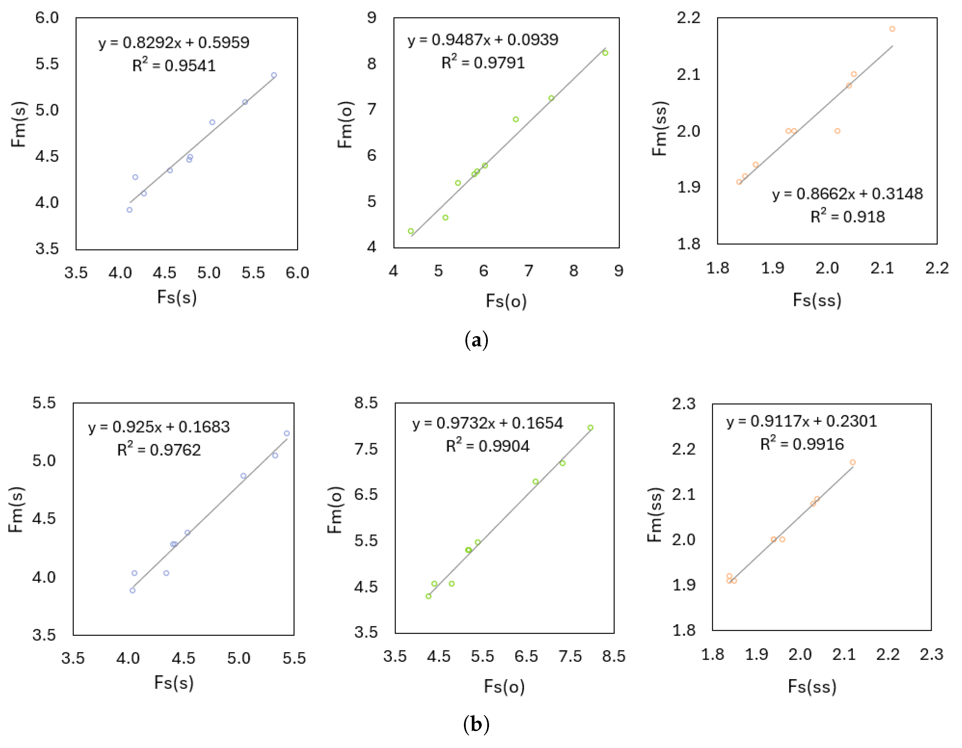
By integrating the FFD-SM into the HSA for GRW design, we evaluated the accuracy of the optimization results across different design cases by comparing the surrogate’s predictions with numerical analyses. To do this, scatter plots (Q-Q) were created for CO and objective functions (Figure 20) to compare the FFD-SM estimates of the sliding, F(s), overturning F(o), and slope stability F(ss) safety factors—, , and —with the corresponding numerical results—, , and , respectively.
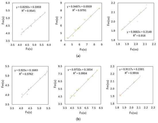
Figure 20.
Q-Q plots for optimum GRW design-based FFD-SM; (a) . (b) (CO.
Also, performance metrics for all models are tabulated in Table 8. FFD-SM obtained confidence values with low error under both objective functions (MAPE ≈ 2% for Fo; ≈3–4% for Fs and Fss). Low RMSE values indicate that FFD-SM can safely replace the numerical solution in optimization loops. MAPE being in the approx 2–4% band for all parameters shows that SM gives results close to the real value in different cases. In both objective functions, the FFD-SM representative is very close to the numerical security factors (most of them > 0.95). This level of compatibility, combined with significantly lower computation costs, supports the use of the agent as a fast and reliable alternative in the optimization process. This efficiency also enables a more comprehensive examination of design variables, which can reveal innovative solutions that traditional methods may not have discovered. In conclusion, the integration of the FFD-SM surrogate can enhance general design optimization strategies across various engineering applications.

Table 8.
Performance metrics for optimal GRW design-based FFD-SM.
5. Discussion
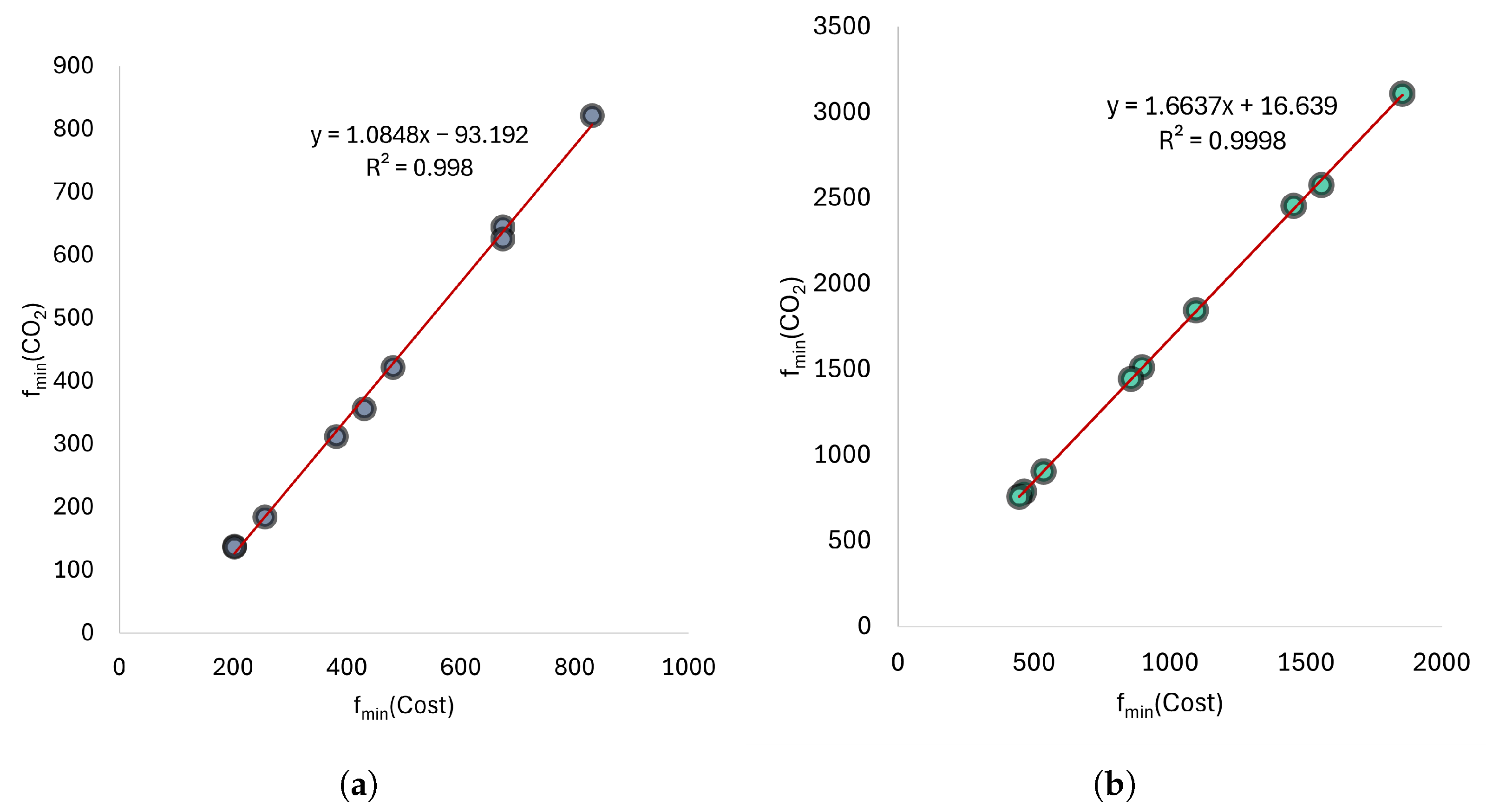
It concluded that there is a linear relationship between cost and CO emissions (Figure 21). The equation for GRW is kgCO with = 0.998, and the equation for CRW is with = 0.999. According to the graphs showing the relationship between CO emissions and cost, lowering the price of the wall design by EUR 1 results in GRW saving approximately 1.085 kg of CO and CRW saving 1.664 kg. The study by Yepes et al. [13] found that this value was 2.28 kg for reinforced concrete retaining walls with varying wall heights, not accounting for the soil properties. This evidence suggests that cost-cutting strategies have a greater impact on reducing CO emissions in GRW designs compared to CRW designs. This study demonstrates the environmental benefits of making design choices that also result in cost savings.
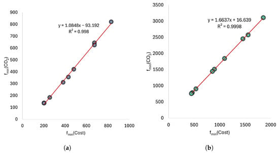
Figure 21.
Relationship between CO emission (kg) and cost (EUR): (a) GRW. (b) CRW.
The optimization analysis efficiently provided us with the best solutions in a shorter time that stay within the set limits, satisfying the constraints of the retaining walls. In this section, the optimal results of CRW and GRW obtained with HSA are examined based on the relationship between cost and CO emissions for various construction items and different design cases. Table 9 and Table 10 display the objective function values of and CO for all GRW and CRW design cases, as well as their construction item units (). The values demonstrate the trade-offs between cost-effectiveness and environmental impact in design scenarios. The tables indicate which construction activity () develops economic and ecological outcomes.

Table 9.
Total amounts of construction items for cost and emission objective functions in optimum GRW design.

Table 10.
Total amounts of construction items for cost and emission objective functions in optimum CRW design.
For both objective functions, the GRW optimal design had a significant average impact of 53% on unit work of soil removal (ER) across design instances (Table 9). The GRW typically contributes 22% to backfilling and 25% to gabion wall construction in cost-optimized designs (). Backfill and gabion wall construction unit operations contribute 15% and 32%, respectively, under optimization for CO.
The best design for CRW had unit work values for the objective functions and CO that were nearly identical, as shown in Table 10—for both objective functions, soil removal operations accounted for 50% of the total, which aligns with the GRW optimal design results. Backfilling of CRW accounts for 17% of all construction for both objective functions. The construction of CRW added 33% to emissions, excluding earthfill and backfill work. According to a literature study by Yepes et al. [13], the construction of CRW is responsible for approximately 40% of emissions. This evaluation aligns with the best results for optimum GRW and CRW. Building a GRW accounts for approximately 25% of all costs, while constructing a cantilever retaining wall accounts for approximately 33%. The construction of GRW results in 32% of (CO) emissions compared to 33% of CRW in terms of total emissions, but less environmental damage is caused in the construction of GRW. For all design cases, GRW resulted in an average emission of 405 kg/m Figure 15, whereas CRW had a value of 1710 kg/m. Although the percentages of backfilling, earth removal, and wall construction were roughly 32–33% for both walls, it is clear that CRW emitted more CO into the atmosphere during construction.
When examining the best and most cost-effective results from optimization analyses for all design cases, we can see that GRWs are more efficient and better for the environment in real-world situations. The scenarios examined in this study corroborate these findings, validating that stone-based solutions, such as MSE and gabion walls, consistently produce lower embodied energy and CO2 emissions compared to concrete-dominated alternatives. These results are also consistent with findings reported in the literature. Previous studies have demonstrated that gabion systems provide significant environmental advantages by utilizing unprocessed stone, thereby decreasing embodied energy and enhancing recyclability. These comparative outcomes, along with material sourcing and lifecycle considerations, further highlight the sustainability benefits of GRWs. In terms of CO emissions, this outcome highlights the benefits of lower cement use, which is consistently recognized as a decisive indicator in life cycle assessment studies [62,63]. Since the stone fill used in GRWs is typically sourced nearby, can be reused, and requires considerably less energy to process than cement, which is the main component of CRWs. Cement production is recognized as one of the most carbon-intensive construction processes, contributing approximately 7–8% of global anthropogenic CO2 emissions [64,65]. This fundamental difference in materials explains why GRW alternatives have much lower embodied energy and carbon footprints.
This significant difference emphasizes the potential for GRW to be a more sustainable construction option. By selecting materials and methods that minimize emissions, the industry can substantially reduce its carbon footprint and contribute to a healthier environment. Recent research has demonstrated that utilizing advanced materials, such as Ultra-High Performance Concrete (UHPC), can yield thinner and more efficient wall sections. This innovation not only has the potential to lower construction costs by using less material, but it also reduces the embodied CO2 emissions associated with producing and transporting heavier concrete structures [66].
Bezerra et al. examined alternative retaining wall designs utilizing geogrid reinforcements, discovering that these structures demonstrate considerably reduced carbon footprints compared to conventional reinforced concrete alternatives. The analysis indicates that redesigning with novel materials can substantially reduce costs and carbon emissions [67]. Pons et al. present a life-cycle assessment that identifies optimization strategies, considering both cost and carbon emissions, which lead to improved structural performance. Their analysis indicates that cantilever retaining walls can be engineered to ensure structural integrity while also mitigating environmental impacts over their operational lifespans [68]. This thorough evaluation is essential, given that traditional concrete manufacturing significantly contributes to global CO emissions; consequently, advancements that decrease concrete volume or enhance durability can result in substantial sustainability improvements [15].
Moreover, research indicates that the application of metaheuristic optimization algorithms can produce optimal design configurations that significantly reduce overall material consumption and expenses, illustrating a viable approach to attaining both economic and ecological objectives [69]. Akış’s research on cost prediction shows that improving the performance of cement through design optimizations can lower the total costs and CO emissions of traditional concrete structures [70]. In conclusion, the comparative analysis of cantilever retaining walls made of concrete demonstrates that strategic design innovations, material advancements, and optimization algorithms are essential in reducing costs and CO emissions. As sustainable building practices evolve, it will be necessary to utilize these methods to minimize the environmental impact of cantilever retaining walls while maintaining their structural integrity and cost-effectiveness.
The results indicate that the construction of GRW has numerous advantages over CRW, including the ease of water drainage due to its ducted structure. In the literature, seasonal variations in groundwater levels and the increasing intensity of rainfall associated with contemporary climate change are identified as factors that adversely impact the stability of cantilever retaining walls due to the additional lateral loads they impose [71]. To mitigate these effects, it is essential to incorporate drainage measures during the construction phase and implement regular maintenance, such as barbacane inspections. Gabion retaining walls, characterized by their permeable structure, inherently address drainage challenges, making them a more effective alternative to cantilever retaining walls in such conditions. By contrast, the drainage measures required for cantilever retaining walls not only increase construction costs but also contribute to greater resource consumption and associated environmental emissions [72]. Hence, gabion walls offer a more sustainable and cost-effective solution for managing the effects of climate-induced hydrological changes.
6. Conclusions
In this research, statistical and mathematical models were formulated as surrogate models using a full factorial design to depict the stability behavior of gabion retaining walls (GRWs). We created 1024 design cases by varying five key parameters. From these, we obtained the safety factors for sliding, overturning, and slope stability. It was demonstrated that the surrogate models, enhanced by the signal-to-noise ratio method, could make accurate and reliable predictions. Using them has numerous benefits, including a significant reduction in the amount of work required for calculations, as there is no longer a need for repeated trial-and-error or complex numerical simulations.
Additionally, these models enhance engineering practice by making optimization tools more effective in real-world projects and by providing designers with quick guidance on selecting stable and efficient wall configurations. Using these surrogate models, the Harmony Search Algorithm (HSA), a type of metaheuristic optimization, was used to compare the economic and environmental performance of GRWs to that of cantilever retaining walls (CRWs). HSA effectively explored the solution space and identified cost-effective and environmentally friendly designs by incorporating surrogate models as constraints into the optimization process. The results showed that GRWs are a better choice for the environment because they produce less CO while still being safe and cost-effective. In general, it is concluded that employing surrogate models based on full factorial design, combined with metaheuristic optimization, constitutes a robust methodology for designing retaining walls. This integrated approach not only reduces the time and money required for analysis and computation but also supports sustainable building practices, enhances engineering, and accelerates the decision-making process for designers. Future research may enhance these surrogate models using sophisticated statistical or machine learning methodologies and extend their application to more versatile gabion geometries, thereby improving sustainability and adaptability in geotechnical engineering.
Supplementary Materials
The following supporting information can be downloaded at https://www.mdpi.com/article/10.3390/math13193216/s1.
Author Contributions
Conceptualization, E.U.; methodology, E.U. and Z.W.G.; software, E.U.; validation, Z.W.G.; investigation, E.U.; writing—original draft preparation, E.U.; review and editing, E.U. and Z.W.G.; visualization, E.U.; supervision, Z.W.G.; funding acquisition, Z.W.G. All authors have read and agreed to the published version of the manuscript.
Funding
This work was supported by the Korea Institute of Energy Technology Evaluation and Planning (KETEP) and the Ministry of Trade, Industry & Energy, Republic of Korea (RS-2024-00441420). This work was carried out during the postdoctoral research of Dr. Esra Uray, supported by the Scientific and Technological Research Council of Türkiye (TÜBİTAK) (1059B192302155). The TUBITAK grant did not provide additional financial support for the publication of this article.
Data Availability Statement
The original contributions presented in this study are included in the article/Supplementary Material. Further inquiries can be directed to the corresponding authors.
Acknowledgments
Esra Uray expresses her deepest gratitude to Özcan Tan, the opinion creator of this study, who has passed away. She also thanks the TUBITAK, the Department of Civil and Environmental Engineering research groups at the University of California, Los Angeles, and Ertugrul Taciroglu for their support.
Conflicts of Interest
The authors declare no conflicts of interest.
Abbreviations
The following abbreviations are used in this manuscript:
| B | Volume of backfilled soil |
| BB–BC | Big bang–big crunch algorithm |
| Unit cost coefficient | |
| CI | Construction items |
| CRW | Cantilever retaining wall |
| Unit and CO emissions coefficient | |
| ER | Volume of earth removed soil |
| FA | Firefly algorithm |
| FFD | Full factorial design |
| FF | Area of foundation formwork |
| GRW overturning safety factor | |
| GRW overturning safety factor | |
| CRW bearing capacity safety factor | |
| CRW bearing capacity safety factor | |
| Surrogate model overturning safety factor | |
| Surrogate model sliding safety factor | |
| Surrogate model slope stability safety factor | |
| GRW sliding safety factor | |
| GRW sliding safety factor | |
| Numerical bearing capacity safety factor | |
| Numerical overturning safety factor | |
| Numerical sliding safety factor | |
| Numerical slope stability safety factor | |
| GRW slope stability safety factor | |
| GRW slope stability safety factor | |
| G | Volume of constructed gabion wall |
| GA | Genetic algorithm |
| GRW | Gabion retaining wall |
| HM | Harmony memory |
| HMCR | Harmony memory considering rate |
| HMS | Harmony memory size |
| HSA | Harmony search algorithm |
| MAPE | Mean Absolute Percentage Error |
| MAE | Mean Absolute Error |
| MaxIter | Maximum iteration |
| MSE | Mean Squared Error |
| PAR | Pitch adjusting rate |
| PSO | Particle swarm optimization |
| Determination coefficient | |
| Relative error | |
| RMSE | Root Mean Squared Error |
| S/N | Signal/Noise ratio |
| SF | Area of stem formwork |
| SM | Surrogate model |
| Std.dev. | Standard deviation |
| TLBO | Teaching–learning-based optimization |
| Amount of construction item |
References
- Jayasree, P.K.; Beena, K.S. Geometric parametric studies on reinforced soil gabion walls. Proc. Inst. Civ. Eng.-Ground Improv. 2015, 164, 21–32. [Google Scholar] [CrossRef]
- Uray, E. Gabion structures and retaining walls design criteria. Adv. Eng. Sci. 2022, 2, 127–134. [Google Scholar]
- Yue, M.; Qu, L.; Zhou, S.; Wu, D.; Chen, Z.; Wen, H. Dynamic response characteristics of shaking table model tests on the gabion reinforced retaining wall slope under seismic action. Geotext. Geomembranes 2024, 52, 167–183. [Google Scholar] [CrossRef]
- Mummadisingh, J.V.; Sengupta, A. Study of the dynamic performance of a gabion wall. Structures 2023, 50, 576–589. [Google Scholar] [CrossRef]
- Chairullah, B.; Sungkar, M.; Munirwan, R.P.; Jamaluddin, K.; Ramadhani, F.F.; Jaya, R.P. The Investigation of Stability on Slopes Utilizing Reinforcement Gabion Walls and Concrete Piles for Mitigating Landslide Disasters. Open Constr. Build. Technol. J. 2024, 18, e18748368310059. [Google Scholar] [CrossRef]
- Tang, V.T.; Fu, D.; Binh, T.N.; Rene, E.R.; Sang, T.T.T.; Singh, R.P. An Investigation on Performance and Structure of Ecological Revetment in a Sub-Tropical Area: A Case Study on Cuatien River, Vinh City, Vietnam. Water 2018, 10, 636. [Google Scholar] [CrossRef]
- Ramli, M.; Karasu, T.; Dawood, E.T. The stability of gabion walls for earth retaining structures. Alex. Eng. J. 2013, 52, 705–710. [Google Scholar] [CrossRef]
- Amato, G.; Obrien, F.; Simms, C.K.; Ghosh, B. Multibody modelling of gabion beams for impact applications. Int. J. Crashworthiness 2013, 18, 237–250. [Google Scholar] [CrossRef]
- Zhao, L.; Gao, L.; Jin, H. Application of gabion slope protection of Nanyang River channel regulation in Tianzhen County. Adv. Mater. Res. 2012, 374–377, 1938–1941. [Google Scholar] [CrossRef]
- Nakazawa, H.; Usukura, K.; Hara, T.; Suetsugu, D.; Kuribayashi, K.; Nishi, T.; Kimura, S.; Shimomura, S. Problems in Earthquake Resistance Evaluation of Gabion Retaining Wall Based on Shake Table Test with Full-Scale Model. J. Disaster Res. 2019, 14, 1154–1169. [Google Scholar] [CrossRef]
- Lin, Y.L.; Zhao, L.; Yang, G.L.; Li, Y.; Zhao, L.H. Engineering behaviors of reinforced gabion retaining wall based on laboratory test. J. Cent. South Univ. Technol. 2010, 17, 1351–1356. [Google Scholar] [CrossRef]
- Gholizadeh, S.; Hasançebi, O. Efficient neural network-aided seismic life-cycle cost optimization of steel moment frames. Comput. Struct. 2024, 301, 107443. [Google Scholar] [CrossRef]
- Yepes, V.; Gonzalez-Vidosa, F.; Alcala, J.; Villalba, P. CO2-optimization design of reinforced concrete retaining walls based on a VNS-threshold acceptance strategy. J. Comput. Civ. Eng. 2012, 26, 378–386. [Google Scholar] [CrossRef]
- Aydogdu, I.; Akın, A. Biogeography Based CO2 and Cost Optimization of RC Cantilever Retaining Walls. In Proceedings of the International Conference on Computing in Civil and Building Engineering, Paris, France, 20–21 July 2015; pp. 1480–1485. [Google Scholar]
- Molina-Moreno, F.; García-Segura, T.; Martí, J.V.; Yepes, V. Optimization of buttressed earth-retaining walls using hybrid harmony search algorithms. Eng. Struct. 2017, 134, 205–216. [Google Scholar] [CrossRef]
- Kayabekir, A.E.; Arama, Z.A.; Bekdaş, G.; Nigdeli, S.M.; Geem, Z.W. Eco-Friendly Design of Reinforced Concrete Retaining Walls: Multi-objective Optimization with Harmony Search Applications. Sustainability 2020, 12, 6087. [Google Scholar] [CrossRef]
- Chau, K.W.; Albermani, F. Knowledge-based system on optimum design of liquid retaining structures with genetic algorithms. J. Struct. Eng. 2003, 129, 1312–1321. [Google Scholar] [CrossRef]
- Khajehzadeh, M.; Taha, M.R.; El-Shafie, A.; Eslami, M. Economic design of retaining wall using particle swarm optimization with passive congregation. Aust. J. Basic Appl. Sci. 2010, 4, 5500–5507. [Google Scholar]
- Camp, C.V.; Akin, A. Design of retaining walls using big bang–big crunch optimization. J. Struct. Eng. 2012, 138, 438–448. [Google Scholar] [CrossRef]
- Sheikholeslami, R.; Khalili, B.G.; Zahrai, S. Optimum cost design of reinforced concrete retaining walls using hybrid firefly algorithm. Int. J. Eng. Technol. 2014, 6, 465. [Google Scholar] [CrossRef]
- Temür, R.; Bekdas¸, G. Teaching learning-based optimization for design of cantilever retaining walls. Struct. Eng. Mech. 2016, 57, 763–783. [Google Scholar] [CrossRef]
- Jiang, P.; Zhou, Q.; Shao, X.; Jiang, P.; Zhou, Q.; Shao, X. Surrogate-Model-Based Design and Optimization; Springer: Berlin/Heidelberg, Germany, 2020. [Google Scholar]
- Qiu, Q.; Li, B.; Feng, P. Optimal design of hydraulic excavator working device based on multiple surrogate models. Adv. Mech. Eng. 2016, 8, 1687814016647947. [Google Scholar] [CrossRef]
- Forrester, A.I.; Keane, A.J. Recent advances in surrogate-based optimization. Prog. Aerosp. Sci. 2009, 45, 50–79. [Google Scholar] [CrossRef]
- Zhang, J.; Chowdhury, S.; Messac, A. An adaptive hybrid surrogate model. Struct. Multidiscip. Optim. 2012, 46, 223–238. [Google Scholar] [CrossRef]
- Wang, C.; Qiang, X.; Xu, M.; Wu, T. Recent advances in surrogate modeling methods for uncertainty quantification and propagation. Symmetry 2022, 14, 1219. [Google Scholar]
- Li, X.; Nishio, M.; Sugawara, K.; Iwanaga, S.; Chun, P.j. Surrogate Model Development for Slope Stability Analysis Using Machine Learning. Sustainability 2023, 15, 10793. [Google Scholar] [CrossRef]
- Zhu, B.; Hiraishi, T.; Pei, H.; Yang, Q. Efficient reliability analysis of slopes integrating the random field method and a Gaussian process regression-based surrogate model. Int. J. Numer. Anal. Methods Geomech. 2021, 45, 478–501. [Google Scholar]
- You, X.; Zhang, M.; Tang, D.; Niu, Z. An active learning method combining adaptive kriging and weighted penalty for structural reliability analysis. Proc. Inst. Mech. Eng. Part O J. Risk Reliab. 2022, 236, 160–172. [Google Scholar]
- Coulomb, C. Essay on maximums and minimums of rules to some static problems relating to architecture. Acad. R. Des. Sci. 1776, 7, 343–382. [Google Scholar]
- Agostini, R. Flexible Gabion Structures in Earth Retaining Works; Officine Maccaferri: Bologna, Italy, 1978. [Google Scholar]
- Braja, M.D.; Sivakugan, N. Principles of Foundation Engineering, 9th ed.; Cengage Learning: Independence, KY, USA, 2017; p. 819. [Google Scholar]
- Meyerhof, G.G. Some Recent Research on the Bearing Capacity of Foundations. Can. Geotech. J. 1963, 1, 16–26. [Google Scholar] [CrossRef]
- Bishop, A.W. The use of the slip circle in the stability analysis of slopes. Geotechnique 1955, 5, 7–17. [Google Scholar]
- GEO5. Geotechnical Software, Version V18; Fine Software: Prague, Czech Republic, 2018.
- Uray, E.; Carbas, S.; Geem, Z.W.; Kim, S. Parameters Optimization of Taguchi Method Integrated Hybrid Harmony Search Algorithm for Engineering Design Problems. Mathematics 2022, 10, 327. [Google Scholar] [CrossRef]
- Tan, O. Investigation of soil parameters affecting the stability of homogeneous slopes using the Taguchi method. Eurasian Soil Sci. 2006, 39, 1248–1254. [Google Scholar] [CrossRef]
- Uray, E.; Tan, Ö.; Çarbaş, S.; Erkan, H. Metaheuristics-based pre-design guide for cantilever retaining walls. Tek. Dergi 2021, 32, 10967–10993. [Google Scholar] [CrossRef]
- Hastie, T.; Tibshirani, R.; Friedman, J. The Elements of Statistical Learning: Data Mining, Inference, and Prediction, 2nd ed.; Springer: New York, NY, USA, 2009; ISBN 978-0-387-84857-0. [Google Scholar] [CrossRef]
- Brady, K.; Kavanagh, J. Analysis of the Stability of Masonry-Faced Earth Retaining Walls; TRL Report 550; Transport Research Laboratory: Crowthorne, UK, 2002. [Google Scholar]
- Rhayma, N.; Khorchani, M.; Breul, P. Reliability and Sensitivity Analysis of Gravity Retaining Wall Stability: Investigating the Effect of Construction Defects. J. Rehabil. Civ. Eng. 2025, 13, 113–129. [Google Scholar]
- Zevgolis, I.E.; Bourdeau, P.L. Probabilistic analysis of retaining walls. Comput. Geotech. 2010, 37, 359–373. [Google Scholar] [CrossRef]
- Shirzadi, N.; Lau, D.; Stylianou, M. Surrogate Modeling for Building Design: Energy and Cost Prediction Compared to Simulation-Based Methods. Buildings 2025, 15, 2361. [Google Scholar] [CrossRef]
- Cao, X.; Lin, S.; Dong, M.; Hu, Q.; Zheng, H. A Surrogate Model for the Rapid Prediction of Factor of Safety in Slopes with Spatial Variability. Mathematics 2025, 13, 1604. [Google Scholar] [CrossRef]
- Geem, Z.W.; Kim, J.H.; Loganathan, G.V. A new heuristic optimization algorithm: Harmony search. Simulation 2001, 76, 60–68. [Google Scholar] [CrossRef]
- Dubey, M.; Kumar, V.; Kaur, M.; Dao, T.P. A systematic review on harmony search algorithm: Theory, literature, and applications. Math. Probl. Eng. 2021, 2021, 5594267. [Google Scholar] [CrossRef]
- Deb, K. An efficient constraint handling method for genetic algorithms. Comput. Methods Appl. Mech. Eng. 2000, 186, 311–338. [Google Scholar] [CrossRef]
- Lagaros, N.D.; Kournoutos, M.; Kallioras, N.A.; Nordas, A.N. Constraint handling techniques for metaheuristics: A state-of-the-art review and new variants. Optim. Eng. 2023, 24, 2251–2298. [Google Scholar] [CrossRef]
- EN 1997-1; Eurocode 7: Geotechnical Design—Part 1: General Rules. British Standards Institution: London, UK, 2004.
- Uray, E.; Çarbaş, S.; Erkan, İ.H.; Olgun, M. Investigation of optimal designs for concrete cantilever retaining walls in different soils. Chall. J. Concr. Res. Lett. 2020, 11, 39–45. [Google Scholar] [CrossRef]
- Catalonia Institute of Construction Technology. BEDEC PR/PCT ITEC Materials Database. 2024. Available online: https://en.itec.cat/database/ (accessed on 20 July 2025).
- Wang, J.; Ouyang, H.; Zhang, C.; Li, S.; Xiang, J. A novel intelligent global harmony search algorithm based on improved search stability strategy. Sci. Rep. 2023, 13, 7705. [Google Scholar] [CrossRef] [PubMed]
- Li, J.; Zhou, Y. Application of Levy flight-based harmony search algorithm for the flexible job shop scheduling. Sci. Rep. 2025, 15, 18124. [Google Scholar] [CrossRef] [PubMed]
- Abualigah, L.; Diabat, A.; Geem, Z.W. A comprehensive survey of the harmony search algorithm in clustering applications. Appl. Sci. 2020, 10, 3827. [Google Scholar] [CrossRef]
- Lee, K.; Geem, Z. A new meta-heuristic algorithm for continuous engineering optimization: Harmony search theory and practice. Comput. Methods Appl. Mech. Eng. 2005, 194, 3902–3933. [Google Scholar] [CrossRef]
- Mahdavi, M.; Fesanghary, M.; Damangir, E. An improved harmony search algorithm for solving optimization problems. Appl. Math. Comput. 2007, 188, 1567–1579. [Google Scholar] [CrossRef]
- Shamsabadi, A.; Xu, S.Y.; Taciroglu, E. A generalized log-spiral-Rankine limit equilibrium model for seismic earth pressure analysis. Soil Dyn. Earthq. Eng. 2013, 49, 197–209. [Google Scholar] [CrossRef]
- Kowalska, M.; Jastrzębska, M. Triaxial tests on weak cohesive soils–some practical remarks (part 1). Arch. Civ. Eng. Environ. 2016, 9, 71–80. [Google Scholar] [CrossRef]
- Li, J.; Tian, Y.; Cassidy, M. Effect of spatial variability on buried footings. In Geotechnical Safety and Risk V; IOS Press: Amsterdam, The Nederland, 2015; pp. 828–833. [Google Scholar]
- Zhu, Y.; Zhang, F.; Jia, S. Embodied energy and carbon emissions analysis of geosynthetic reinforced soil structures. J. Clean. Prod. 2022, 370, 133510. [Google Scholar] [CrossRef]
- Uray, E.; Carbas, S.; Olgun, M. Investigation of Parametric Effect in Optimum Retaining Wall Design Using Harmony Search Algorithm. In Harmony Search and Nature Inspired Optimization Algorithms; Kim, A., Deep, J., Deep, K., Geem, Z., Sadollah, A., Yadav, A., Eds.; Lecture Notes on Data Engineering and Communications Technologies; Springer: Singapore, 2022; Volume 140, pp. 435–445. [Google Scholar] [CrossRef]
- Balasbaneh, A.T.; Marsono, A.K.; Kadir, M.R.A.; Huat, L.K. Assessing the Life Cycle Study of Alternative Earth-Retaining Walls from an Environmental and Economic Viewpoint. J. Clean. Prod. 2021, 279, 123689. [Google Scholar] [CrossRef]
- Araújo Junior, L.P.V.D.; Bueno, C.; Silva, J.L.D. Life Cycle Assessment and Circularity Indicators of Earth-Retaining Walls and Mechanically Stabilized Earth. Sustainability 2025, 17, 3769. [Google Scholar] [CrossRef]
- Andrew, R.M. Global CO2 emissions from cement production. Earth Syst. Sci. Data 2018, 10, 195–217. [Google Scholar] [CrossRef]
- Scrivener, K.; John, V.; Gartner, E. Eco-efficient cements: Potential, economically viable solutions for a low-CO2 cement-based materials industry. Cem. Concr. Res. 2018, 114, 2–26. [Google Scholar] [CrossRef]
- Nematollahi, B.; Voo, Y.L.; R, R.S.M. Structural behavior of precast Ultra-High Performance Fiber Reinforced Concrete (UHPFRC) cantilever retaining walls: Part II—Full scale experimental testing. KSCE J. Civ. Eng. 2014, 18, 1481–1495. [Google Scholar] [CrossRef]
- de Almeida Bezerra, J.V.; Mota, T.G.; da Silva Andrade, H.M.L.; de Andrade, L.P.; Vigoderis, R.B. Comparative study of retaining walls aiming to optimize carbon footprint. Rev. Ibero-Am. Ciências Ambient. 2020, 11, 460–467. [Google Scholar]
- Pons, J.J.; Penadés-Plà, V.; Yepes, V.; Martí, J.V. Life cycle assessment of earth-retaining walls: An environmental comparison. J. Clean. Prod. 2018, 192, 411–420. [Google Scholar] [CrossRef]
- Kaveh, A.; Hamedani, K.B.; Bakhshpoori, T. Optimal design of reinforced concrete cantilever retaining walls utilizing eleven meta-heuristic algorithms: A comparative study. Period. Polytech. Civ. Eng. 2020, 64, 156–168. [Google Scholar] [CrossRef]
- Akis, E. Optimum cost prediction of reinforced concrete cantilever retaining walls. Buildings 2023, 13, 2409. [Google Scholar] [CrossRef]
- Öser, C.; Sayin, B. Geotechnical assessment and rehabilitation of retaining structures collapsed partially due to environmental effects. Eng. Fail. Anal. 2021, 119, 104998. [Google Scholar] [CrossRef]
- Chen, Y.; Gao, Y.; Ng, C.W. A new capillary barrier system for retaining wall backfilled with fine-grained soil. Comput. Geotech. 2020, 118, 103324. [Google Scholar] [CrossRef]
Disclaimer/Publisher’s Note: The statements, opinions and data contained in all publications are solely those of the individual author(s) and contributor(s) and not of MDPI and/or the editor(s). MDPI and/or the editor(s) disclaim responsibility for any injury to people or property resulting from any ideas, methods, instructions or products referred to in the content. |
© 2025 by the authors. Licensee MDPI, Basel, Switzerland. This article is an open access article distributed under the terms and conditions of the Creative Commons Attribution (CC BY) license (https://creativecommons.org/licenses/by/4.0/).

