A FIG-IWOA-BiGRU Model for Bus Passenger Flow Fluctuation Trend and Spatial Prediction

Abstract

To capture bus passenger flow fluctuations and address the problems of slow convergence and high error in machine learning parameter optimization, this paper develops an improved Whale Optimization Algorithm (IWOA) integrated with a Bidirectional Gated Recurrent Unit (BiGRU). First, a Logistic–Tent chaotic mapping is introduced to generate a diverse and high-quality initial population. Second, a hybrid mechanism combining elite opposition-based learning and Cauchy mutation enhances population diversity and reduces premature convergence. Third, a cosine-based adaptive convergence factor and inertia weight strategy improve the balance between global exploration and local exploitation. Based on the correlation analysis between bus passenger flow and weather condition data in Harbin, and combined with the fluctuation characteristics of bus passenger flow, the data were divided into windows with a 7-day weekly cycle and processed by fuzzy information granulation to obtain three groups of fuzzy granulated window data, namely LOW, R, and UP, representing the fluctuation trend and spatial characteristics of bus passenger flow. The IWOA was employed to optimize and solve parameters such as the hidden layer weights and bias vectors of the BiGRU, thereby constructing a bus passenger flow fluctuation trend and spatial prediction model based on FIG-IWOA-BiGRU. Simulation experiments with 21 benchmark functions and real bus data verified its effectiveness. Results show that IWOA significantly improves optimization accuracy and convergence speed. For bus passenger flow forecasting, the average MAE, RMSE, and MAPE of LOW, R, and UP data are 2915, 3075, and 8.1%, representing improvements over existing classical models. The findings provide reliable decision support for bus scheduling and passenger travel planning.

1. Introduction

Bus passenger flow serves as the basis for bus operation management departments to formulate network planning and vehicle scheduling plans. By establishing the relationship between bus passenger flow and its influencing factors, and exploring the fluctuation patterns of randomness, time variation, and imbalance in passenger flow, an accurate prediction model of passenger flow fluctuations can be constructed. This enables reasonable forecasting of fluctuation trends and spatial distribution of passenger flow, thereby providing a theoretical foundation for developing bus operation scheduling plans. Meanwhile, it also facilitates passengers in planning travel routes and times more effectively, improves operational efficiency, and ensures the service level and quality of bus services.

Mei Z et al. [1] pointed out that factors such as weather conditions, bus stop information, bus passenger flow change rate, and time and date have significant impacts on bus passenger flow. Chen D et al. [2] established a nonlinear relationship between bus passenger flow and factors such as the number of bus stops, road network density, and the number of companies, revealing the influencing mechanisms of passenger flow changes. Zhu C et al. [3] found that the land-use characteristics surrounding bus stops have a significant impact on bus passenger flow. Fang X et al. [4] examined the correlation between bus IC card passenger flow attributes and travel time, and proposed a passenger flow forecasting method based on the classification of travel attributes. Chen E et al. [5] analyzed the time-series characteristics of bus IC card passenger flow data and developed an ARIMA-based forecasting model. To further analyze the seasonal periodic patterns of bus passenger flow, Milenković M et al. [6] proposed a Seasonal Autoregressive Integrated Moving Mean (SARIMA)-based bus passenger flow forecasting method. Cheng G et al. [7] developed a Short Time Series Clustering–Seasonal Autoregressive Integrated Moving Mean (STSC-SARIMA) model for bus passenger flow forecasting. However, the above studies primarily fit linear regression relationships between bus passenger flow and influencing factors using historical data samples, without adequately addressing the spatiotemporal dynamics and nonlinear characteristics of bus passenger flow. This may result in the omission of certain spatiotemporal dynamic influencing factors and their relationships during parameter calibration, thereby reducing the accuracy and generalization capability of bus passenger flow forecasting results [8].

To investigate the spatiotemporal dynamic complexity and nonlinear relationships between bus passenger flow and factors such as weather conditions, commercial land-use ratio, points of interest (POI), bus stop density, and characteristics of bus and road networks under large-scale data samples, and to explore the characteristic patterns of influencing factors and the spatiotemporal distribution of bus passenger flow to improve forecasting accuracy and robustness, Yu L et al. [9] examined the impact of land-use characteristics on bus passenger flow and proposed a bus passenger flow forecasting model based on the least squares support vector machine. Xu X et al. [10] developed a combined forecasting model integrating time series analysis and support vector machines for bus passenger flow. Li Y et al. [11] proposed a bus passenger flow forecasting method based on the kernel extreme learning machine (KELM), which effectively improved the accuracy of forecasting results. Yazıcıoğlu C et al. [12] introduced an LSTM-based bus passenger flow forecasting method, and the results showed that incorporating weather conditions helps enhance the accuracy and applicability of the forecasts. Zhang Y et al. [13] compared the forecasting accuracy of existing machine learning models and found that bidirectional forecasting models, such as those based on BiLSTM and BiGRU, outperform unidirectional models in both accuracy and robustness.

To further integrate the spatiotemporal distribution features of the built environment, bus stop density, and bus and road networks, and to improve the accuracy and applicability of bus passenger flow forecasting, Cao B et al. [14] proposed a hybrid forecasting method based on convolutional neural network–long short-term memory (CNN-LSTM) by incorporating factors such as commercial land-use ratio, points of interest (POI), and bus stop density. This method effectively extracts the spatiotemporal features of bus passenger flow, reduces model computational complexity, and achieves higher forecasting accuracy compared to LSTM networks. Baghbani A et al. [15] developed a traffic-aware multi-step graph neural network (TMS-GNN)-based method for bus passenger flow forecasting, which considers bus stop connectivity and urban traffic operation characteristics to significantly improve both the accuracy and applicability of forecasts. Lv W et al. [16] constructed an extreme gradient boosting (XGBoost) model for bus passenger flow forecasting by incorporating POI information. Yu J et al. [17] proposed an interpretable bus passenger flow forecasting method based on CatBoost, which not only improves forecasting accuracy but also reveals the interaction mechanisms between influencing factors and forecast accuracy. These studies have effectively enhanced the accuracy and robustness of bus passenger flow forecasting by exploring the complex spatiotemporal dynamic relationships and distribution characteristics between bus passenger flow and influencing factors. However, they often rely on manually setting parameters for machine learning models, which can limit the precision and efficiency of parameter optimization.

To further improve the accuracy and efficiency of bus passenger flow forecasting, Nagaraj N et al. [18] examined factors such as bus type, the locations of route terminals, passenger numbers, and headways, and proposed a forecasting method based on a greedy hierarchical algorithm combined with a long short-term memory (LSTM) neural network. Sun F et al. [19] explored the spatiotemporal distribution patterns of bus passenger flow using IC card data and developed a forecasting model based on a nonlinear autoregressive network with exogenous inputs (NARX) optimized by a genetic algorithm. Li C et al. [20], considering the volatility, nonlinearity, and periodicity of bus passenger flow, applied a clustering algorithm to segment passenger flow data and constructed a forecasting model based on a particle swarm optimization–support vector machine (PSO-SVM). Bus passenger flow forecasting models based on GWO-SVM [21] and whale optimization-Attention-Bidirectional Gated Recurrent Unit (BiGRU) [22] have also demonstrated high prediction accuracy and strong generalization capability, as intelligent optimization algorithms are used to fine-tune machine learning hyperparameters.

The whale optimization algorithm (WOA) in intelligent optimization exhibits advantages such as simple structure, few parameters, and high accuracy and convergence speed in optimization solving [23], and has been widely applied in areas including path planning [24] and machine learning parameter optimization [25]. However, due to the use of an initialization strategy in the optimization process, WOA often suffers from uneven population distribution. Moreover, the linearly decreasing convergence factor during population position updating tends to cause an imbalance between global search and local exploitation, leading to problems such as being trapped in local optima, insufficient solution accuracy, and slow convergence speed. To address these issues, Prasad D [26] and Duan Y et al. [27] improved the population initialization of WOA by adopting Logistic and Circle chaotic mappings, thereby enhancing population diversity and quality and improving optimization speed and convergence accuracy. Similarly, Darvish Falehi A [28] and Paul C et al. [29] applied chaotic mappings to improve WOA population initialization, balancing the relationship between global search and local exploitation, enhancing optimization accuracy and speed, and strengthening WOA’s capability in solving complex engineering problems.

To address the issue that the Whale Optimization Algorithm (WOA) is prone to premature convergence to local optima, Li M [30] and Chakraborty S et al. [31] improved WOA by employing an elite opposition-based learning strategy. This approach enhanced population diversity and local exploration capability, increased the probability of feasible solutions approaching the optimal solution during the optimization process, and avoided premature convergence caused by limited exploration ability.

Regarding the problem that the linearly decreasing convergence factor in WOA cannot effectively balance the relationship between global search and local exploitation, thereby reducing solution accuracy and convergence speed, Anitha J [32] and Yue Y et al. [33] introduced cosine functions to improve convergence factors and inertia weights. This effectively balanced global and local search abilities, enhancing both solution accuracy and convergence speed. Chakraborty S et al. [34] suggested that improving the coefficient vector in the position update mechanism could significantly enhance the exploration capability in the early stage and the exploitation capability in the later stage. Wang H [35] and Yang W et al. [36] used nonlinear functions and dynamic convergence factors to improve the linear convergence factor of WOA, strengthening global and local search capabilities while reducing the risks of premature convergence and insufficient accuracy. Ju C et al. [37] integrated chaotic mapping, nonlinear convergence factors, and Cauchy mutation as a hybrid strategy to improve WOA. This increased population diversity and quality, effectively balanced global and local search abilities, and overcame the issues of insufficient accuracy, slow convergence, and susceptibility to local optima.

Existing studies mainly focus on examining the impacts of factors such as weather conditions, built environment, and the characteristics of bus and road networks on bus passenger flow, and on developing models aimed at improving the point-in-time forecasting accuracy of bus passenger flow, while neglecting its randomness, time variation, and imbalance. The use of intelligent optimization algorithms to tune machine learning parameters can avoid the limitations of manual parameter setting, which often results in insufficient accuracy and applicability of forecasting results.

Therefore, to address the problems of WOA being easily trapped in local optima, insufficient solution accuracy, and slow convergence speed, this study adopts a Logistic–Tent combined chaotic mapping to initialize the population of WOA, thereby increasing population diversity and quality; an elite opposition-based learning and Cauchy mutation hybrid mechanism is adopted to overcome premature convergence and the tendency of WOA to fall into local optima. Moreover, improved convergence factors and inertia weights are introduced to enhance the population position update mechanism, effectively balancing the relationship between global search and local exploitation, and improving both solution accuracy and convergence speed of WOA. Based on bus passenger flow data from Harbin, the study analyzes the correlations between passenger flow, weather conditions, and passenger attributes, applies fuzzy information granulation (FIG) to the passenger flow data, and employs the improved WOA (IWOA) to optimize BiGRU parameters, thereby developing a FIG-IWOA-BiGRU model for forecasting bus passenger flow fluctuation trends and spatial distribution. By considering the impacts of passenger travel randomness and uncertainty on bus passenger flow, the model extends forecasting results from point predictions to spatial predictions. Meanwhile, the use of a hybrid-strategy-improved WOA prevents the algorithm from falling into local optima and suffering from slow convergence, which could otherwise lead to poor BiGRU prediction performance and long computation times, thus addressing the limitations in bus passenger flow data forecasting applications.

The remainder of this paper is organized as follows: Section 1 analyzes the fluctuation characteristics of bus passenger flow and its influencing factors. Section 2 briefly introduces fuzzy information granulation and the whale optimization algorithm. Section 3 presents in detail the strategies and functions of the improved whale optimization algorithm, and constructs the FIG-IWOA-BiGRU model for forecasting bus passenger flow fluctuation trends and spatial distribution. Section 4 provides the results of numerical simulation experiments based on 21 benchmark test functions and discusses the advantages of the improved whale optimization algorithm compared with other metaheuristic algorithms. The results of the FIG-IWOA-BiGRU bus passenger flow fluctuation trend and spatial forecasting model are then presented, followed by a comparative analysis of the accuracy and applicability of the proposed model and existing models.

2. Bus Passenger Flow Fluctuation Characteristics and Influencing Factors Analysis

2.1. Analysis of Bus Passenger Flow Fluctuation Characteristics

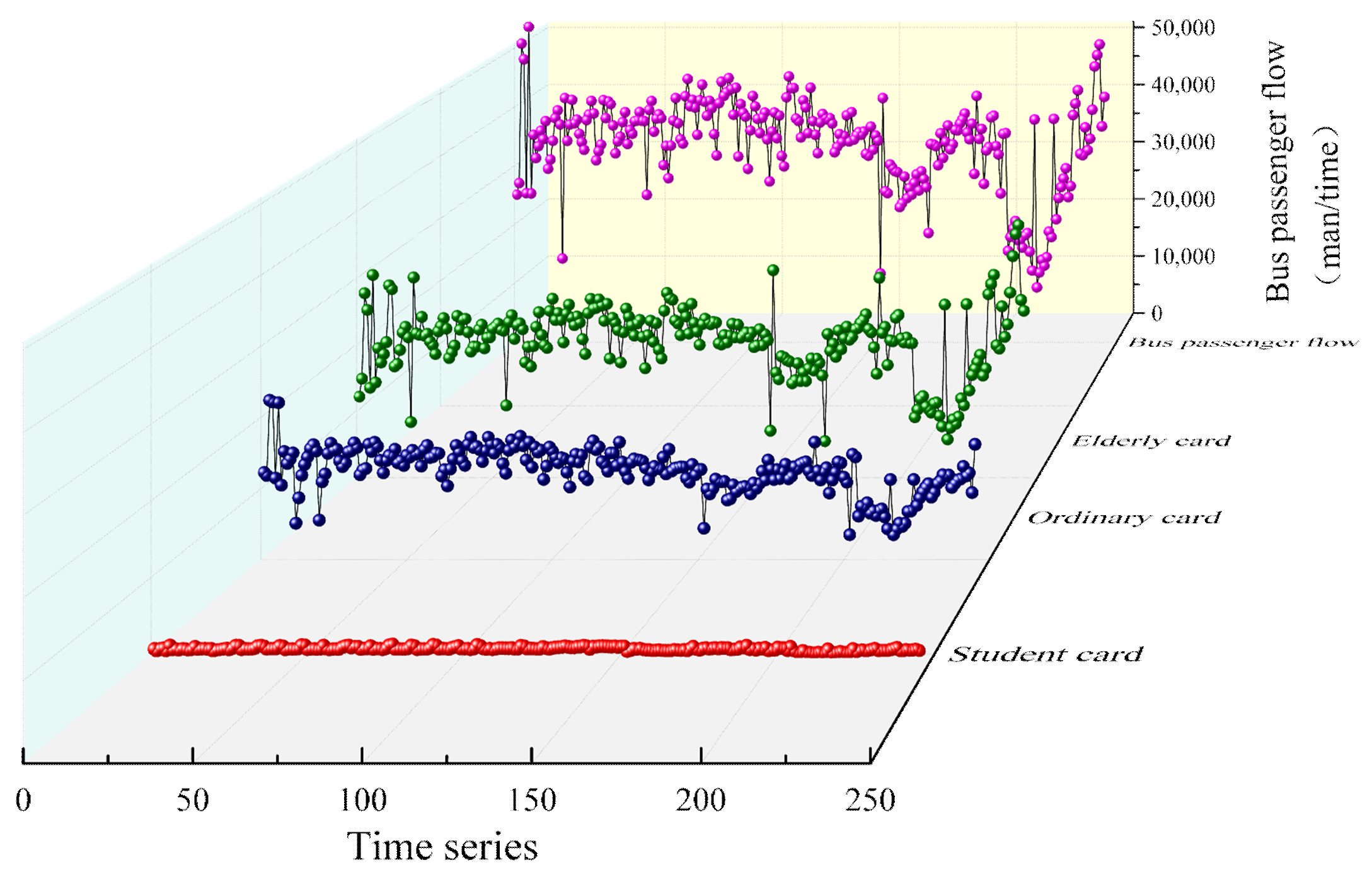
The fluctuation characteristics of bus passenger flow represent the overall fluctuation trend and spatial variation range of passenger flow within a given period. As shown in the time series of bus passenger flow fluctuations in Figure 1, the fluctuation trends and spatial ranges of different IC card types vary across different periods; however, they share the following characteristics:

1. Temporal and spatial attributes—The fluctuation characteristics of bus passenger flow reflect changes in passenger travel demand within a given period, as well as the influence of land-use characteristics and the degree of development around bus routes on travel demand.

2. Object and condition attributes—These characteristics treat the passenger flow of a bus route as a whole and examine changes in passenger travel demand from a macro perspective. New fluctuation patterns in bus passenger flow emerge only when passengers’ travel purposes and modes change.

3. Predictability—From the perspective of residents’ travel demand and mode choice, the fluctuation characteristics of bus passenger flow reflect the service level of bus operations and can be analyzed and forecast based on historical data patterns.

2.2. Principles for Selecting Influencing Factors of Bus Passenger Flow

The selection of influencing factors for bus passenger flow aims to reduce the workload of data collection and processing while ensuring the accuracy of forecasting model results. The main principles include the following:

1. Scientific validity—The selected factors should objectively reflect changes in their impact on passenger travel. For example, passengers have an optimal preference for weather conditions; the degree of deviation from this optimal value is inversely proportional to travel comfort. Therefore, indicators such as clothing index, wind scale, and daily Mean temperature can better capture the seasonal variations in temperature and their effects on passenger travel.

2. Availability—The selected factors should be accessible and calculable. For instance, air quality index, relative humidity, and clothing index can be obtained and computed from meteorological websites.

3. Sensitivity—The selected factors should have a significant impact on the fluctuation characteristics and trends of bus passenger flow.

2.3. Analysis of Influencing Factors of Bus Passenger Flow

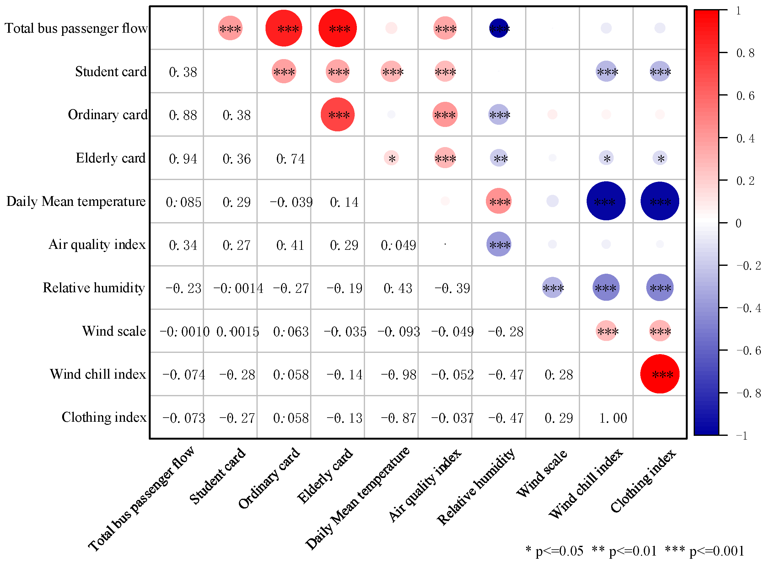
Liu J et al. [38] argued that considering weather conditions can help improve the accuracy of bus passenger flow forecasting. To further analyze the relationship between bus passenger flow and weather conditions, influencing factors were selected for the fluctuation trend and spatial prediction datasets of bus ridership. The research data mainly consist of bus IC card records and corresponding weather conditions in Harbin from 1 March 2021 to 31 October 2021, covering a total of 245 days. Considering that both bus IC card data and weather condition data contain partial temporal gaps, a time series method was employed to repair and complete the missing data. The Pearson correlation coefficient in binary interval variable correlation analysis was employed to examine the degree of correlation between bus passenger flow and weather-related influencing factors, and the results are shown in Figure 2.

Existing studies suggest that when the correlation coefficient between two influencing factors exceeds 0.95, the factors are considered highly correlated, and one of them should be removed [38]. As shown in Figure 2, the correlation coefficients among the factors selected in this study are $\left|{\rho }_{X,Y}\right|<0.95$, except that the wind chill index shows correlations higher than 0.95 with both daily Mean temperature and clothing index. The correlations among the remaining factors are within the threshold range. Therefore, daily Mean temperature, air quality index, relative humidity, wind scale, and clothing index were selected as the influencing factors for bus passenger flow forecasting.

3. Fuzzy Information Granulation and Whale Optimization Algorithm

3.1. Fuzzy Information Granulation

Given the randomness and uncertainty of bus passenger flow and weather data, the fuzzy granulation method based on fuzzy set theory is applied to determine the fuzzy granulation window and perform information fuzzy granulation processing on bus passenger flow data. The number of fuzzy granulation windows is determined according to the characteristics of bus passenger flow data, dividing them into several fuzzy granulation sub-windows according to a fixed rule length. The purpose of information fuzzy granulation is to obtain reasonable fuzzy information granules for each window while retaining the valid information of the original window data, thereby simplifying the spatial dimensionality of the model. The triangular membership function and the Gaussian membership function are commonly used fuzzy information granulation methods. The membership function for fuzzy information granulation is typically determined using histogram plotting. The histogram of bus passenger flow data is shown in Figure 3. As illustrated in Figure 3, the triangular membership function provides a better fuzzy information granulation of bus passenger flow data. Moreover, compared with trapezoidal and Gaussian membership functions, the triangular membership function offers the advantages of computational simplicity, efficiency, and rapid modeling.

Thus, this study adopts the triangular membership function for bus passenger flow information granulation, which is expressed as Equation (1):

$$A(x,a,m,b)=\left\{\begin{array}{ll}0,& x<a\\ {\displaystyle \frac{x-a}{m-a}},& a\le x\le m\\ {\displaystyle \frac{b-x}{b-m}},& m<x\le b\\ 0,& x>b\end{array}\right.$$

(1)

where $a$, $m$, and $b$ represent the minimum value, mean value, and maximum value, respectively, of the fluctuations in the original sample data after window granulation.

3.2. Whale Optimisation Algorithm

3.2.1. Encircling Prey

The WOA was proposed by Mirjalili et al. [39] in 2016 as an intelligent optimization algorithm consisting of mathematical models such as encircling prey, spiral bubble-net attacking, and random search for prey. Encircling prey refers to the assumption that, due to the uncertainty of the optimal position in the data samples, the model considers the position of the current sample with the highest fitness as the target position and uses it as a reference for other samples to update their own positions. The formula is as follows:

$$\overrightarrow{D}=\left|C\cdot \overrightarrow{X^{*}}(t)-\overrightarrow{X}(t)\right|$$

(2)

$$\overrightarrow{X}(t+1)=\overrightarrow{X^{*}}(t)-A\cdot \overrightarrow{D}$$

(3)

where $t$ denotes the current iteration number, $\overrightarrow{X^{*}}$ is the position vector of the best individual, $\overrightarrow{X}$ is the position vector, and the coefficient vectors A and C are calculated as follows:

$$A=2a\cdot r_1-a$$

(4)

$$C=2r_2$$

(5)

where $a$ is a coefficient that decreases linearly from 2 to 0 as the iterations progress, and $r_1$ and $r_2$ are random variables in the range [0, 1].

3.2.2. Spiral Bubble-Net Attacking

The spiral bubble-net attacking mainly simulates the process of updating the positions of other samples toward the position of the optimal sample through spiral position updating and a shrinking encircling mechanism. Since spiral position updating and the shrinking encircling mechanism occur simultaneously during the spiral bubble-net attacking process, this mathematical model assumes that each occurs with a probability of 50%. The formula is as follows:

$$\overrightarrow{X}(t+1)=\overrightarrow{X^{*}}(t)-A\cdot \overrightarrow{D},\hspace{1em}\hspace{1em}\hspace{1em}\hspace{1em} \mathrm{if} p<0.5$$

(6)

$$\overrightarrow{X}(t+1)=\overrightarrow{D^{’}}\cdot e^{bl}\cdot \cos (2\pi l)+\overrightarrow{X^{*}}(t),\hspace{1em}\mathrm{if} p\ge 0.5$$

(7)

where $b$ is a constant defining the shape of the spiral, and $l$ and $p$ are random numbers in the range [−1,1].

3.2.3. Random Search for Prey

The random search for prey updates positions by performing a random search based on the locations of data samples. This mathematical model assumes that when A > 1, the position of a sample is randomly updated according to the characteristics of the data samples, in order to enhance global search capability. The formula is as follows:

$$\overrightarrow{D}=\left|C\cdot \overrightarrow{X_{rand}}-X\right|$$

(8)

$$\overrightarrow{X}(t+1)=\stackrel{⇢}{X_{rand}}-A\cdot \overrightarrow{D}$$

(9)

where $\stackrel{⇢}{X_{rand}}$ is an individual randomly selected from the current population.

4. Improved Whale Optimization–Bidirectional Gated Recurrent Unit

4.1. Logistic–Tent Combined Mapping Initialization

A randomly and uniformly distributed initial population helps expand the search space of the algorithm, improving its convergence speed and solution accuracy [40]. In the absence of any prior information, the whale optimization algorithm generates the initial population randomly within the search space, which can easily lead to uneven distribution of individual positions and a reduced search space. Therefore, this study combines Logistic and Tent chaotic mappings to construct a Logistic–Tent combined mapping. This combined mapping integrates the strong spatial ergodicity of Logistic mapping with the fast iteration speed, low autocorrelation, and strong applicability of Tent mapping. Such a combination helps improve the uniformity and ergodicity of population spatial distribution in WOA during the optimization of bus passenger flow data, thereby overcoming the tendency to fall into local optima and enhancing the convergence speed and accuracy in solving BiGRU parameters. The formula is as follows:

$$z(t+1)=\left\{\begin{array}{ll}r{z}_t\left(1-z(t)\right)+\left(4-r\right)z(t),& 0<z(t)\le 0.3\\ r{z}_t\left(1-z(t)\right)+\left(4-r\right)\left(1-z(t)\right),& 0.3<z(t)<1\end{array}\right.$$

(10)

where $z(t)$ is the value after the t-th iteration, and $r$ is a random parameter in the range (0, 4).

4.2. Elite Opposition-Based Learning and Cauchy Mutation Hybrid Mechanism

4.2.1. Elite Opposition-Based Learning

The opposition-based learning (OBL) strategy, proposed by Tizhoosh [30] in 2005, is a learning strategy that, based on the current feasible solution, evaluates its opposite solution and selects the better feasible solution from the current and opposite solutions, with the aim of increasing the probability of the optimal feasible solution approaching the global optimum. This strategy can effectively improve the diversity and quality of the algorithm’s population and prevent the algorithm from prematurely falling into a local optimum. It has been widely applied to the improvement of various intelligent optimization algorithms and has achieved favorable results.

The opposition-based learning strategy assumes that the current feasible solution of the population is $\mathit{X}=(x_1,x_2,\cdots ,x_d)$, where $d$ is the dimension of the search space and $x_j\in \left[a_j,b_j\right]$. Its opposite solution is $\overline{\mathit{X}}=(\overline{x_1},\overline{x_2},\cdots ,\overline{x_d})$, where $\overline{x_j}=\omega (a_j+b_j)-x_j$, and $\omega$ is a generalized coefficient uniformly distributed in [0, 1].

The elite opposition-based learning strategy [31] is an improved approach proposed to address the issue in the opposition-based learning strategy, where the generated opposite solution is more difficult to reach the global optimum within the current search space. It has been widely applied to the improvement of various algorithms and has achieved favorable results. Assuming that the local extremum point corresponding to a general individual in the current population is an elite individual ${\mathit{X}}_{i,j}^e=(X_{i,1}^e,X_{i,2}^e,\cdots ,X_{i,d}^e)(i=1,2,3,\cdots ,d)$, its opposite solution $\overline{{\mathit{X}}_{i,j}^e}=(\overline{X_{i,1}^e},\overline{X_{i,2}^e},\cdots \overline{X_{i,d}^e})$ can be expressed as

$$\overline{{\mathit{X}}_{i,j}^e}=K^{*}({\alpha }_j+{\beta }_j)-{\mathit{X}}_{i,j}^e$$

(11)

where $K$ is a dynamic coefficient in the range (0, 1), and ${\mathit{X}}_{i,j}^e\in \left[{\alpha }_j,{\beta }_j\right]$, ${\alpha }_j=\min (X_{i,j})$, ${\beta }_j=\min (X_{i,j})$, ${\alpha }_j$ and ${\beta }_j$ are dynamic boundaries that overcome the limitation of fixed boundaries in preserving search experience. These dynamic boundaries enable the elite opposite solution to be located within a narrow search space, thereby improving the convergence performance of the algorithm. If the operation causes ${\mathit{X}}_{i,j}^e$ to cross the boundary and become an infeasible solution, it can be reset using the method of random generation defined in Equation (12).

$$\overline{{\mathit{X}}_{i,j}^e}=rand({\alpha }_j,{\beta }_j)$$

(12)

4.2.2. Cauchy Mutation

Given that the Cauchy distribution function has a slow decay along the horizontal axis and a heavy-tailed property, it can be used to optimize the best position of whale individuals in the WOA. This allows rapid perturbation of the current optimal solution obtained during the optimization process, enabling fast search for feasible solutions within the bus passenger flow data space, and enhancing the algorithm’s global search capability as well as its ability to escape local optima [38]. When the WOA converges to the global optimal solution, the updated position of the optimal whale individual after Cauchy mutation perturbation is

$$X_{newbest}^j=X_{best}^j+X_{best}^j\times Cauchy(0,1)$$

(13)

where $X_{newbest}^j$ is the optimal whale position after Cauchy perturbation, $X_{best}^j$ is the optimal whale position before Cauchy perturbation, and $Cauchy(0,1)$ is a random value generated from the standard Cauchy distribution.

4.2.3. Hybrid Mechanism

The hybrid mechanism expands the search range of the WOA in the bus passenger flow data space through elite opposition-based learning, enabling the exploration of more potential optimal solutions to improve the convergence speed and accuracy in optimizing BiGRU parameters. Cauchy mutation is mainly used to randomly perturb the optimal whale position, enhancing its ability to escape from local optima and accelerating the solution process of BiGRU parameters for bus passenger flow forecasting. The dynamic updating method of the optimal whale position under the hybrid mechanism is as follows:

$$\overline{{\mathit{X}}_{newbest,i,j}^e}=\left\{\begin{array}{l}{\displaystyle \frac{(a_j+b_j)}{2}}+{\displaystyle \frac{(a_j+b_j)}{2n}}-{\displaystyle \frac{X_{best,i,j}^j}{n}}, \lambda <0.5\\ {\mathit{X}}_{best,i,j}^e+X_{best,i,j}^e\times Cauchy(0,1), \lambda \ge 0.5\end{array}\right.$$

(14)

where λ is a random number in the range [0, 1].

4.3. Improved Convergence Factor and Inertia Weight

For swarm intelligence optimization algorithms, it is necessary to balance the relationship between global search and local exploitation. Failure to achieve this balance may cause the algorithm to converge prematurely to a local optimum or to converge slowly. Global search means that the population explores a wide search space with relatively large search steps and range, which can reduce the probability of falling into a local optimum. Local exploitation requires the population to perform refined searches within a local space, thereby avoiding the loss of the theoretical optimum due to excessively large search steps [23]. As a swarm intelligence optimization algorithm, WOA also depends critically on balancing global search and local exploitation. From Equations (3), (6) and (8), it can be seen that this balance largely depends on the value of A. From Equation (4), it follows that changes in the convergence factor $a$ determine the value of A.

Given that the convergence factor in WOA decreases linearly and does not adequately balance the relationship between global search and local exploitation, this study incorporates the characteristics of the cosine function to improve the convergence factor formula as follows:

$$a=2-2\cos ({\displaystyle \frac{\pi }{2}}·{\displaystyle \frac{t}{t_{\max }}})$$

(15)

Given that WOA continuously updates the leader’s position, it is prone to falling into local optima. To address this issue, this study introduces an inertia weight into the whale position updating process to increase the probability of WOA escaping from local optima. The improved whale position updating formula is as follows:

$$\overrightarrow{X}(t+1)=\phi \overrightarrow{X^{*}}(t)-A\cdot \overrightarrow{D},\left|A\right|<1,p<0.5$$

(16)

$$\overrightarrow{X}(t+1)=\phi \overrightarrow{X_{rand}}-A\cdot \overrightarrow{D} \left|A\right|\ge 1,p<0.5$$

(17)

$$\overrightarrow{X}(t+1)=\overrightarrow{D^{\prime }}\cdot e^{bl}\cdot \cos (2\pi l)+\phi \overrightarrow{X^{*}}(t),p\ge 0.5$$

(18)

where $\phi$ is the inertia weight, calculated as

$$\phi (t+1)={\phi }_{\max }-({\phi }_{\max }-{\phi }_{\min })·\cos ({\displaystyle \frac{t}{t_{\max }}}\pi )$$

(19)

4.4. Bidirectional Gated Recurrent Unit

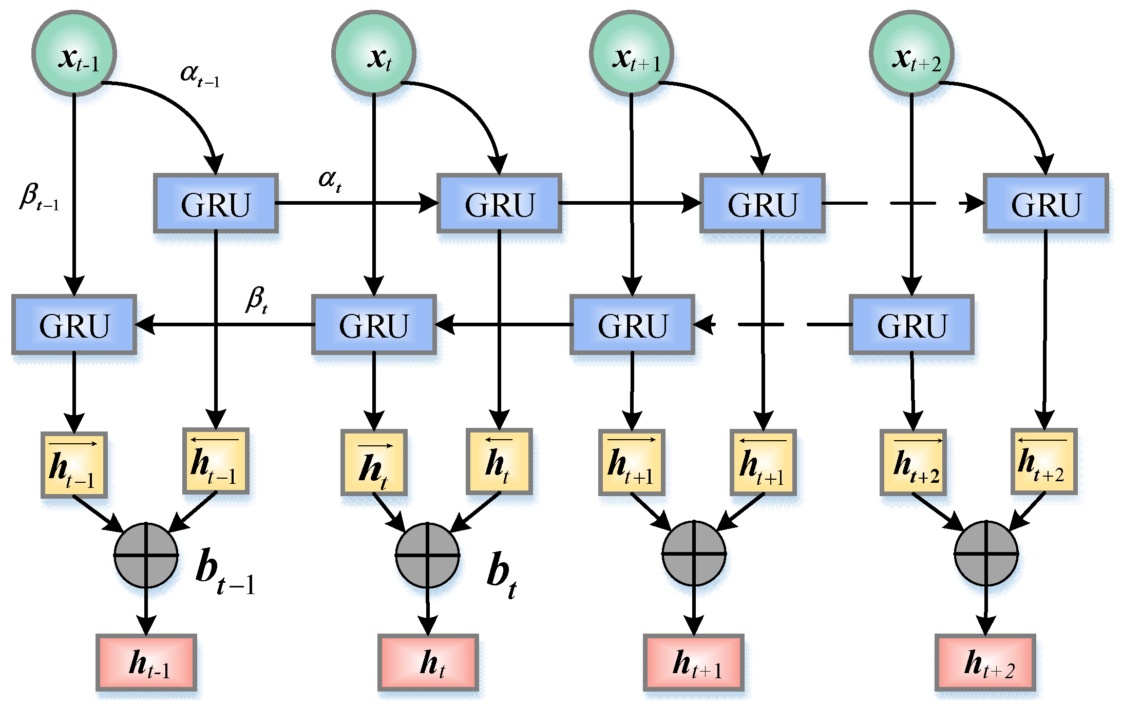
As shown in Figure 4, the bidirectional gated recurrent unit (BiGRU) consists of several forward and backward GRUs that operate in opposite temporal directions and are independent of each other. Compared with GRU, BiGRU offers bidirectional modeling, accurate temporal annotation, and strong data feature extraction capabilities, while having fewer network parameters than LSTM. The calculation of the hidden layer units within BiGRU is shown in Equation (20):

$$\left\{\begin{array}{ll}\overrightarrow{{\mathit{h}}_t}& =GRU({\mathit{x}}_t,\overrightarrow{{\mathit{h}}_{t-1}})\\ \overleftarrow{{\mathit{h}}_t}& =GRU({\mathit{x}}_t,\overleftarrow{{\mathit{h}}_{t-1}})\\ {\mathit{h}}_t& ={\alpha }_t\overrightarrow{{\mathit{h}}_t}+{\beta }_t\overleftarrow{{\mathit{h}}_t}+{\mathit{b}}_t\end{array}\right.$$

(20)

where $GRU(\cdot )$ is the gated recurrent unit, ${\mathit{x}}_t$ is the input value, $\overrightarrow{{\mathit{h}}_t}$ and ${\alpha }_t$ are the forward hidden state and weight, $\overleftarrow{{\mathit{h}}_t}$ and ${\beta }_t$ are the backward hidden state and weight, and ${\mathit{b}}_t$ is the hidden layer bias vector.

4.5. FIG-IWOA-BiGRU Model Prediction Process

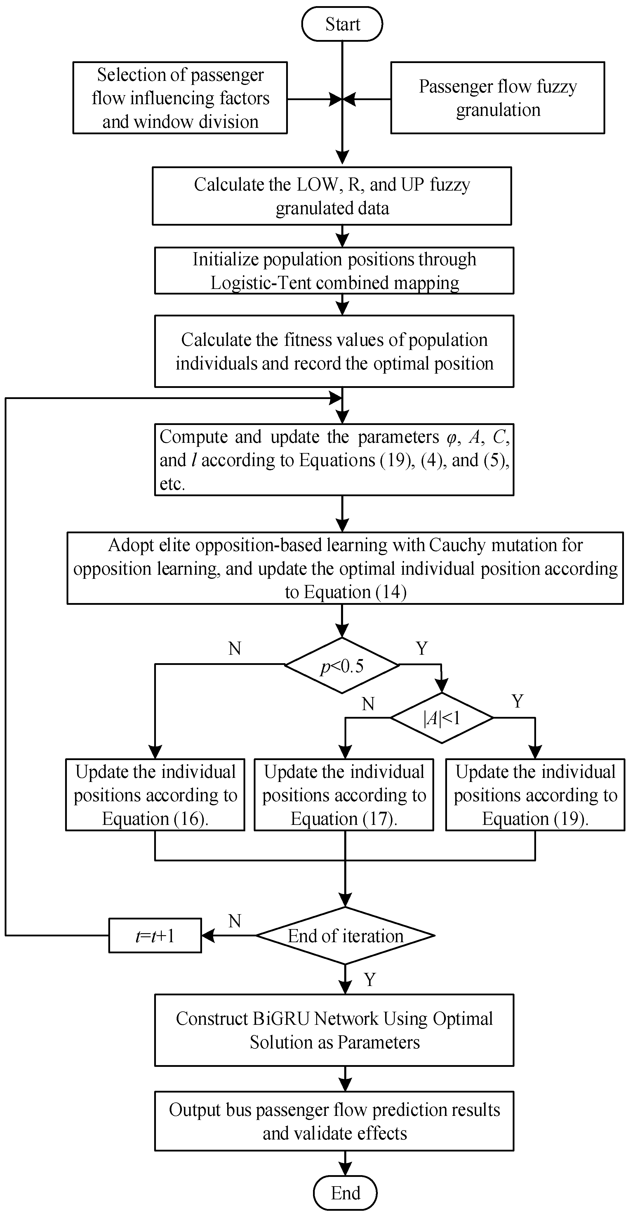
Based on the analysis results of bus passenger flow fluctuation characteristics and influencing factors, the bus passenger flow data are divided into fuzzy granulation windows with a period of 7 days per week, and triangular fuzzy membership functions are used for fuzzy granulation processing. The fuzzy-granulated bus passenger flow data are used as input samples, and the hybrid-strategy–improved WOA is employed to optimize the hyperparameters of the BiGRU model, which is then trained to obtain the bus passenger flow fluctuation trend and spatial prediction model. The steps of the FIG-IWOA-BiGRU bus passenger flow fluctuation trend and spatial prediction model are as follows, and the process is shown in Figure 5.

1.Select the influencing factors of bus passenger flow and compile the dataset; divide the bus passenger flow data into fuzzy granulation windows with a period of 7 days per week.

2. Apply a triangular fuzzy membership function to fuzzify the bus passenger flow window time series sample data, and compute the fuzzified window time series samples after fuzzy information granulation.

3. Set the improved WOA population size to 30 and the number of iterations to 500.

4. Generate the initial population within the search space using the Logistic–Tent combined mapping.

5. Calculate the fitness values of the individuals in the population and record the optimal position $\stackrel{⇢}{X(t)}$.

6. Apply the elite opposition-based learning and Cauchy mutation hybrid mechanism for opposition-based learning, evaluate and select the solution according to the objective function’s fitness value, update the solutions in each dimension using this method, and update the position of the optimal whale individual according to Equation (14).

7. Update parameter $\phi$ according to Equation (19), and update parameters $a$, $A$, $C$, and $l$ accordingly.

8. Compare the value of $\left|A\right|$ and the random value $p$ with 0.5, then select the corresponding position updating formula. If $p<0.5$ and $\left|A\right|<1$, update the current position according to Equation (16); if $p<0.5$ and $\left|A\right|\ge 1$, perform random prey search according to Equation (17); if $p\ge 0.5$, update the current position according to Equation (18).

9. Check whether the algorithm has reached the maximum number of iterations. If so, stop the iterations and output the optimal position and fitness value; otherwise, repeat steps (4)–(8).

10. Output the global optimal solution obtained by the IWOA and use it as the optimal parameter set to construct the BiGRU.

11. Use the FIG-IWOA-BiGRU model to forecast bus passenger flow fluctuation trends and spatial ranges, and verify the prediction performance.

5. Numerical Simulation and Forecasting Results Analysis

5.1. Numerical Simulation Results

To verify the effectiveness of the IWOA, 21 typical benchmark test functions were selected for numerical simulation. The results of 30 simulation runs were comprehensively compared with those of WOA, Grey Wolf Optimizer Algorithm (GWO), Particle Swarm Optimization Algorithm (PSO), and Genetic Algorithm (GA). All numerical simulations were conducted in a Windows 11 environment with 32 GB of RAM (Kingston Technology, Fountain Valley, CA, USA) and a 12th Gen Intel(R) Core(TM) i7-12700 processor (2.10 GHz) (Intel Corporation, Santa Clara, CA, USA), using MATLAB R2023b as the programming language. In the numerical simulation experiments, the maximum number of iterations was set to 500, and the population size was 30. Other parameter settings of each algorithm model are provided in

Table 1. Test function Information.

Algorithm	Value
IWOA	Parameter a decreases from 2 to 0 following a cosine function, p,r1,r2 ∈ [0, 1], spiral constant b = 1, and l ∈ [−1, 1]
WOA	Parameter a decreases linearly from 2 to 0, p,r1,r2 ∈ [0,1], spiral constant b = 1, and l ∈ [−1,1]
GWO	Parameter a decreases linearly from 2 to 0, r1,r2 ∈ [0,1]
PSO	Learning factors C1 = C2 = 2, particle velocity Vmax = 2, Vmin = −2, and inertia weight Wmax = 0.8, Wmin = 0.2
GA	Crossover probability Pc = 0.8, mutation probability Pm = 0.2.

. Among the 21 benchmark test functions, f₁–f₇ are high-dimensional unimodal benchmark test functions, f₈–f₁₃ are high-dimensional multimodal benchmark test functions, and f₁₄–f₂₁ are fixed-dimensional composite multimodal benchmark test functions, as detailed in

Table 2. Relevant values of test functions.

Type	Function	Dimension	Search Range	Theoretical Optimal Value
Unimodal Benchmark test functions	$f_1(x)={\displaystyle \sum _{i=1}^n{x}_i^2}$	30	$[-100,100]$	0
	$f_2(x)={\displaystyle \sum _{i=1}^{\mathrm{n}}\left|x_i\right|}+{\displaystyle \prod _{i=1}^n\left|x_i\right|}$	30	$[-10,10]$	0
	$f_3(x)={{\displaystyle \sum _{i=1}^n\left({\displaystyle \sum _{j-1}^i{x}_j}\right)}}^2$	30	$[-100,100]$	0
	$f_4(x)={\max }_i\left\{\left|x_i\right|,1\le i\le n\right\}$	30	$[-100,100]$	0
	$f_5(x)={\displaystyle \sum _{i=1}^{n-1}\left[100{\left(x_{i+1}-x_i^2\right)}^2+{\left(x_i-1\right)}^2\right]}$	30	$[-30,30]$	0
	$f_6(x)={\displaystyle \sum _{i=1}^n{\left(\left[x_i+0.5\right]\right)}^2}$	30	$[-100,100]$	0
	$f_7(x)={\displaystyle \sum _{i=1}^{n}i{x}_i^4}+random[0,1)$	30	$[-1.28,1.28]$	0
Multimodal benchmark test functions	$F_8(x)={\displaystyle \sum _{i=1}^n-x_i\sin \left(\sqrt{\left|x_i\right|}\right)}$	30	$[-500,500]$	$-418.98\times Di{m}^n$
	$F_9(x)={\displaystyle \sum _{i=1}^n\left[x_i^2-10\cos \left(2\pi x_i\right)+10\right]}$	30	$[-5.12,5.12]$	0
	$F_{10}(x)=-20\exp \left(-0.2\sqrt{{\displaystyle \frac{1}{n}}{\displaystyle \sum _{i=1}^n{x}_i^2}}\right)-\exp \left({\displaystyle \frac{1}{n}}{\displaystyle \sum _{i=1}^n\cos \left(2\pi x_i\right)}\right)+20+e$	30	$[-32,32]$	0
	$F_{11}(x)={\displaystyle \frac{1}{4000}}{\displaystyle \sum _{i=1}^n{x}_i^2-{\displaystyle \prod _{i=1}^n\cos \left(\frac{x_i}{\sqrt{i}}\right)}}+1$	30	$[-600,600]$	0
	$\begin{array}{l}{F}_{12}(x)={\displaystyle \frac{\pi }{n}}\left\{10\sin (\pi y_1)+{\displaystyle \sum _{i=1}^{n-1}{\left(y_i-1\right)}^2\left[1+10{\sin }^2(\pi y_{i+1})\right]+{\left(y_n-1\right)}^2}\right\}\\ +{\displaystyle \sum _{i=1}^{n}u(x_i,10,100,4)}\\ y_i=1+{\displaystyle \frac{x_i+1}{4}}\\ u(x_i,a,k,m)=\left\{\begin{array}{ll}k{(x_i-a)}^m& \hspace{1em}{x}_i>a\\ 0& \hspace{1em}-a<x_i<a\\ k{(-x_i-a)}^m& \hspace{1em}{x}_i<-a\end{array}\right.\end{array}$	30	$[-50,50]$	0
	$\begin{array}{l}{F}_{13}(x)=0.1\left\{{\sin }^2\left(3\pi x_1\right)+{\displaystyle \sum _{i=1}^n{\left(x_i-1\right)}^2\left[1+{\sin }^2\left(3\pi x_i+1\right)\right]}\right.\\ \left.+{(x_n-1)}^2\left[1+{\sin }^2\left(2\pi x_n\right)\right]\right\}+{\displaystyle \sum _{i=1}^{n}u\left(x_i,5,100,4\right)}\end{array}$	30	$[-50,50]$	0
Composite multimodal benchmark test functions	$F_{14}(x)={\left({\displaystyle \frac{1}{500}}+{\displaystyle \sum _{j=1}^{25}\frac{1}{j+{\displaystyle \sum _{i=1}^2{(x_i-a_{ij})}^6}}}\right)}^{-1}$	2	$[-65,65]$	1
	$F_{15}(x)={{\displaystyle \sum _{i=1}^{11}\left[a_i-\frac{x_1(b_i^2+b_1{x}_2)}{b_i^2+b_1{x}_3+x_4}\right]}}^2$	4	$[-5,5]$	0.0003
	$F_{16}(x)={\left(x_2-{\displaystyle \frac{5.1}{4{\pi }^2}}{x}_1^2+{\displaystyle \frac{5}{\pi }}{x}_1-6\right)}^2+10\left(1-{\displaystyle \frac{1}{8\pi }}\right)\cos x_1+10$	2	$[-5,5]$	0.398
	$\begin{array}{l}{F}_{17}(x)=\left[1+{(x_1+x_2+1)}^2(19-14x_1+3x_1^2-14x_2+6x_1{x}_2+3x_2^2)\right]\\ \times \left[30+{(2x_1-3x_2)}^2\times (18-32x_1+12x_1^2+48x_2-36x_1{x}_2+27x_2^2)\right]\end{array}$	2	$[-2,2]$	3
	$F_{18}(x)=-{\displaystyle \sum _{i=1}^4{c}_i\exp \left(-{\displaystyle \sum _{j=1}^6{a}_{ij}{(x_j-p_{ij})}^2}\right)}$	6	$[0,1]$	−3.32
	$F_{19}(x)=-{\displaystyle \sum _{i=1}^5{\left[(X-a_i){(X-a_i)}^T+c_i\right]}^{-1}}$	4	$[0,10]$	−10.1532
	$F_{20}(x)=-{\displaystyle \sum _{i=1}^7{\left[(X-a_i){(X-a_i)}^T+c_i\right]}^{-1}}$	4	$[0,10]$	−10.4028
	$F_{21}(x)=-{\displaystyle \sum _{i=1}^{10}{\left[(X-a_i){(X-a_i)}^T+c_i\right]}^{-1}}$	4	$[0,10]$	−10.5363

. The numerical simulation results are presented in terms of statistical parameters such as mean, standard deviation, best fitness, and worst fitness. The statistical results for the different types of benchmark test functions are shown in

Table 3. Unimodal Benchmark test functions.

Function	Indicator	IWOA	WOA	GWO	PSO	GA
f1	Best	4.3 × 10−133	1.5 × 10−85	7.6 × 10−30	2.9 × 10	2.1 × 103
	Worst	4.4 × 10−110	2.3 × 10−73	5.1 × 10−27	5.5 × 102	1.6 × 104
	Mean	1.5 × 10−111	1.8 × 10−74	1.3 × 10−27	3.3 × 102	8.5 × 103
	Standard	8.1 × 10−111	5.6 × 10−74	1.4 × 10−27	1.3 × 102	4.0 × 103
f2	Best	1.0 × 10−82	1.8 × 10−59	1.7 × 10−17	6.9	2.3 × 10
	Worst	5.5 × 10−67	6.1 × 10−50	7.4 × 10−16	4.5 × 10	6.0 × 10
	Mean	1.8 × 10−68	2.8 × 10−51	1.3 × 10−16	1.7 × 10	4.0 × 10
	Standard	1.0 × 10−67	1.2 × 10−50	1.3 × 10−16	9.3	9.5
f3	Best	7.9 × 10−9	7.1 × 103	9.3 × 10−12	1.8 × 103	2.2 × 104
	Worst	4.0 × 10−3	7.2 × 104	6.2 × 10−1	5.0 × 104	5.2 × 104
	Mean	1.4 × 10−4	4.5 × 104	3.3 × 10−2	1.1 × 104	3.7 × 104
	Standard	7.3 × 10−4	1.4 × 104	1.2 × 10−1	1.1 × 104	7.9 × 103
f4	Best	2.2 × 10−31	2.9 × 10−2	1.1 × 10−7	4.5	5.1 × 10
	Worst	2.5 × 10−23	8.9 × 10	5.4 × 10−6	1.4 × 10	8.6 × 10
	Mean	1.2 × 10−24	5.5 × 10	1.1 × 10−6	8.7	6.9 × 10
	Standard	4.6 × 10−24	2.9 × 10	1.1 × 10−6	2.6	8.3
f5	Best	2.6 × 10	2.7 × 10	2.8 × 10	7.6 × 102	2.1 × 104
	Worst	2.9 × 10	2.9 × 10	2.9 × 10	4.9 × 104	6.4 × 106
	Mean	2.7 × 10	2.8 × 10	2.9 × 10	1.3 × 104	1.1 × 106
	Standard	6.7 × 10−1	4.3 × 10−1	4.9 × 10−2	1.3 × 104	1.7 × 106
f6	Best	2.2 × 10−6	5.6 × 10−2	2.4 × 10−1	7.4 × 10	3.4 × 103
	Worst	3.1 × 10−4	1.0	1.8	9.5 × 102	2.4 × 104
	Mean	6.3 × 10−5	4.2 × 10−1	8.3 × 10−1	3.8 × 102	1.0 × 104
	Standard	7.2 × 10−5	2.4 × 10−1	3.7 × 10−1	2.1 × 102	6.1 × 103
f7	Best	7.3 × 10−5	1.9 × 10−4	2.2 × 10−4	3.3 × 10−2	1.5 × 10−1
	Worst	4.5 × 10−3	7.2 × 10−3	4.2 × 10−3	1.3 × 10	2.0
	Mean	1.1 × 10−3	2.3 × 10−3	1.8 × 10−3	1.2	6.8 × 10−1
	Standard	1.1 × 10−3	2.1 × 10−3	9.8 × 10−4	2.8	5.1 × 10−1

,

Table 4. Multimodal benchmark test functions.

Function	Indicator	IWOA	WOA	GWO	PSO	GA
f8	Best	−1.3 × 104	−1.3 × 104	−7.3 × 103	−9.2 × 103	−2.8 × 103
	Worst	−5.0 × 103	−5.7 × 103	−3.4 × 103	−4.6 × 103	−1.0 × 103
	Average	−1.2 × 104	−1.0 × 104	−5.9 × 103	−7.1 × 103	−2.1 × 103
	Standard	1.9 × 103	2.1 × 103	8.4 × 102	1.1 × 103	4.9 × 102
f9	Best	0.0	0.0	5.7 × 10−14	1.2 × 102	1.6 × 102
	Worst	0.0	1.1 × 10−13	7.0	2.4 × 102	3.0 × 102
	Average	0.0	3.8 × 10−15	1.1	1.9 × 102	2.6 × 102
	Standard	0.0	2.1 × 10−14	1.9	3.5 × 10	3.0 × 10
f10	Best	4.4 × 10−16	4.4 × 10−16	7.5 × 10−14	3.8	1.9 × 10
	Worst	7.5 × 10−15	4.0 × 10−15	1.5 × 10−13	8.2	2.1 × 10
	Average	3.2 × 10−15	3.0 × 10−15	1.0 × 10−13	5.7	2.0 × 10
	Standard	2.7 × 10−15	1.6 × 10−15	1.7 × 10−14	1.0	3.7 × 10−1
f11	Best	0.0	0.0	0.0	1.7	2.1 × 10
	Worst	0.0	1.7 × 10−1	5.9 × 10−2	6.6	1.7 × 102
	Average	0.0	9.9 × 10−3	4.9 × 10−3	3.9	9.1 × 10
	Standard	0.0	3.8 × 10−2	1.2 × 10−2	1.2	4.6 × 10
f12	Best	2.3 × 10−7	3.7 × 10−3	1.9 × 10−2	1.1	9.8 × 10−1
	Worst	4.5 × 10−5	9.7 × 10−2	8.4 × 10−2	1.3 × 10	3.3 × 10
	Average	7.1 × 10−6	2.4 × 10−2	4.3 × 10−2	5.8	1.1 × 10
	Standard	8.8 × 10−6	1.8 × 10−2	1.8 × 10−2	2.9	6.8
f13	Best	1.1 × 10−1	3.2 × 10−1	5.0 × 10−5	6.8	1.3 × 10
	Worst	1.3 × 10	1.2	2.6	4.4 × 10	3.8 × 106
	Average	5.8 × 10−1	7.4 × 10−1	1.1	1.9 × 10	2.3 × 105
	Standard	3.1 × 10−1	2.5 × 10−1	1.0	9.7	8.1 × 105

and

Table 5. Composite multimodal benchmark test functions.

Function	Indicator	IWOA	WOA	GWO	PSO	GA
f14	Best	1.0	1.0	1.0	1.0	1.0
	Worst	1.0	1.1 × 10	1.3 × 10	1.3 × 10	1.0
	Average	1.0	3.0	3.0	9.1	1.0
	Standard	1.2 × 10−10	2.9	3.0	5.0	2.8 × 10−10
f15	Best	3.3 × 10−4	3.1 × 10−4	8.0 × 10−4	9.8 × 10−4	3.1 × 10−4
	Worst	2.2 × 10−3	2.0 × 10−2	2.0 × 10−2	2.4 × 10−2	2.3 × 10−2
	Average	6.5 × 10−4	3.7 × 10−3	6.3 × 10−3	7.5 × 10−3	5.5 × 10−3
	Standard	3.7 × 10−4	7.6 × 10−3	7.6 × 10−3	7.4 × 10−3	8.9 × 10−3
f16	Best	4.0 × 10−1	4.0 × 10−1	4.0 × 10−1	4.0 × 10−1	5.9 × 10
	Worst	4.0 × 10−1	4.0 × 10−1	4.0 × 10−1	4.0 × 10−1	8.1 × 10
	Average	4.0 × 10−1	4.0 × 10−1	4.0 × 10−1	4.0 × 10−1	6.9 × 10
	Standard	8.7 × 10−6	3.3 × 10−5	7.0 × 10−5	1.6 × 10−5	6.5
f17	Best	−3.9	−3.9	−3.9	−3.1	−3.7
	Worst	−3.9	−3.8	−3.9	−3.1	−2.5
	Average	−3.9	−3.9	−3.9	−3.1	−3.1
	Standard	2.8 × 10−3	1.5 × 10−2	1.7 × 10−3	2.7 × 10−5	3.6 × 10−1
f18	Best	−3.3	−3.3	−3.3	−3.2	−2.7
	Worst	−3.1	−2.4	−2.6	−1.1	−6.1 × 10−1
	Average	−3.3	−3.2	−3.1	−2.6	−1.6
	Standard	7.1 × 10−2	1.9 × 10−1	1.8 × 10−1	7.9 × 10−1	5.3 × 10−1
f19	Best	−1.0 × 10	−1.0 × 10	−1.0 × 10	−1.0 × 10	−3.8
	Worst	−5.1	−2.6	−2.6	−5.1	−9.6 × 10−1
	Average	−1.0 × 10	−7.3	−8.5	−8.2	−2.1
	Standard	9.2 × 10−1	2.9	2.6	2.5	7.8 × 10−1
f20	Best	−1.0 × 10	−1.0 × 10	−1.0 × 10	−1.0 × 10	−3.4
	Worst	−5.1	−1.8	−2.8	−3.7 × 10-1	−1.0
	Average	−1.0 × 10	−7.8	−9.4	−7.4	−2.1
	Standard	9.7 × 10−1	3.1	2.2	3.4	6.2 × 10−1
f21	Best	−1.1 × 10	−1.1 × 10	−1.1 × 10	−1.1 × 10	−3.8
	Worst	−9.9	−2.4	−2.4 × 10	−5.1	−1.2
	Average	−1.0 × 10	−7.1	−1.0 × 10	−8.4	−2.1
	Standard	1.5 × 10−1	3.2	2.1	2.7	6.5 × 10−1

.

Table 3 presents the statistical results of best fitness, worst fitness, mean fitness, and standard deviation for unimodal benchmark test functions. As test functions with a unique global optimum, unimodal benchmark functions are primarily used to evaluate the exploitation capability of intelligent optimization algorithms. According to Table 3, the IWOA demonstrates superior exploitation ability. For functions f₁, f₂, f₄, and f₆, all statistical results of the IWOA outperform those of other intelligent optimization algorithms. For functions f₃, f₅, and f₇, IWOA ranks as the second-best algorithm. Therefore, the strategies proposed in this paper significantly enhance WOA, enabling the improved algorithm to achieve stronger exploitation ability compared with other intelligent optimization algorithms.

Compared with unimodal benchmark test functions, multimodal benchmark test functions have the characteristic of containing many local optima as the function dimension increases. This characteristic is effective for evaluating the exploration capability of intelligent optimization algorithms. According to the data in Table 4, the improved WOA demonstrates better exploration capability on multimodal benchmark test functions compared with algorithms such as WOA, GWO, PSO, and GA. This is mainly because the hybrid mechanism of elite opposition-based learning and Cauchy mutation effectively prevents the algorithm from falling into local optima and increases the probability of feasible solutions approaching the global optimum.

Composite multimodal benchmark test functions are more complex in structure and contain multiple local minima within their domains. They are commonly used to test an algorithm’s ability to balance global search and local exploitation. Only when an intelligent optimization algorithm achieves an appropriate balance between exploration and exploitation can it effectively overcome the problem of falling into local optima. According to the results in Table 5, the improved WOA exhibits superior capability in balancing global search and local exploitation on composite multimodal benchmark test functions compared with WOA, GWO, PSO, and GA. The improved balance performance of the algorithm mainly benefits from the enhancement of the convergence factor using the cosine function and the application of inertia weight in updating whale positions.

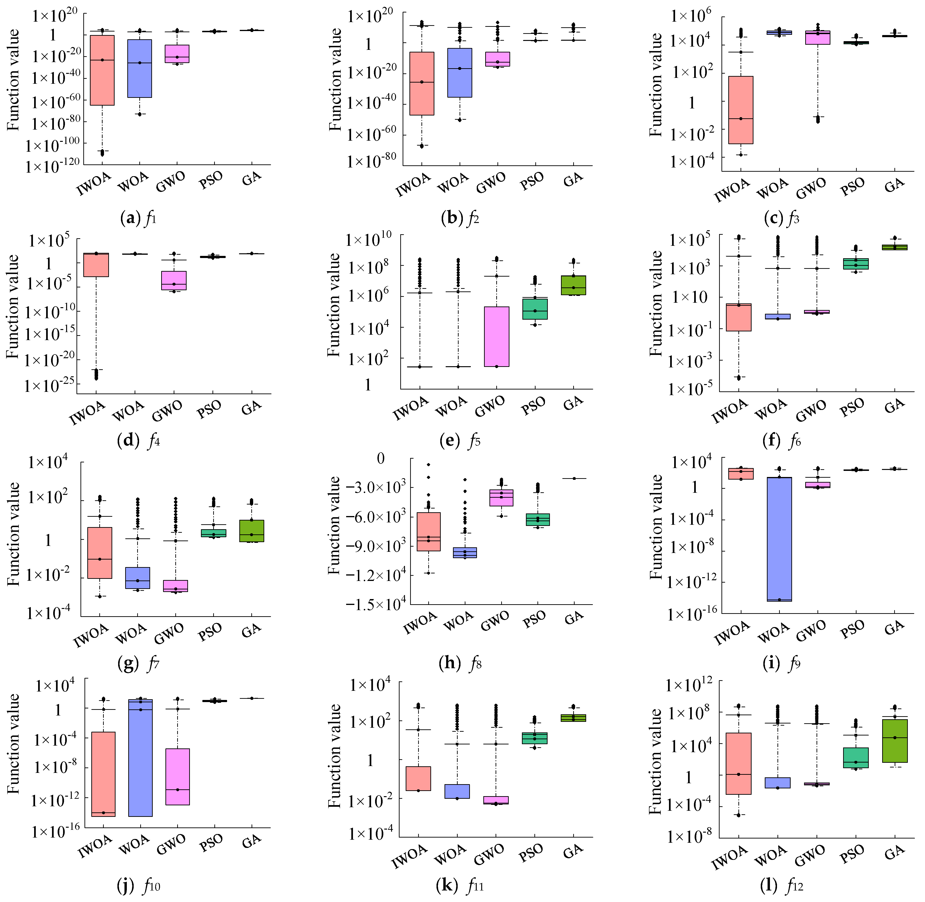
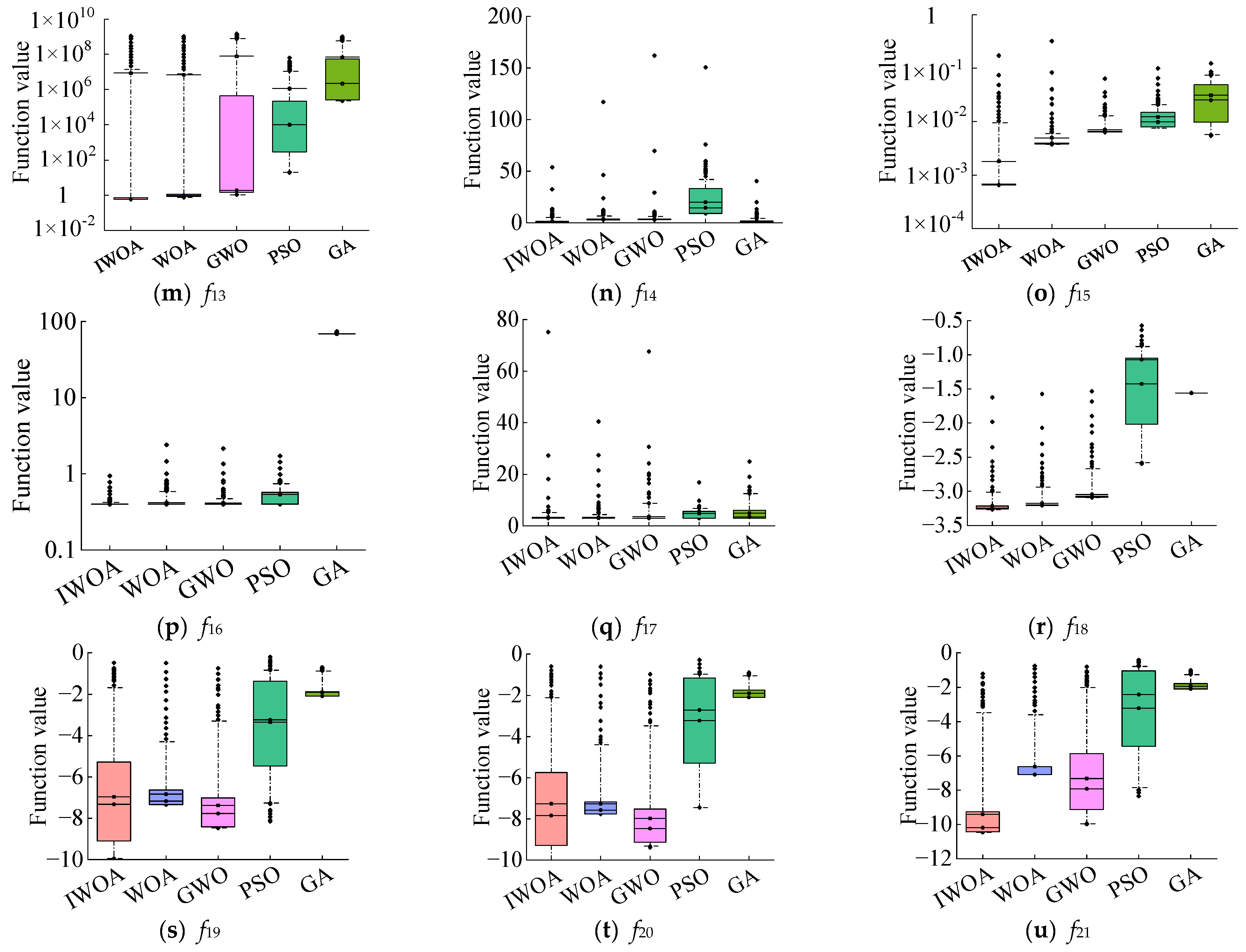
To further analyze the distribution characteristics of the IWOA’s numerical simulation results, box plots were drawn based on the results of each algorithm independently solving the benchmark test functions 30 times, as shown in Figure 6. In Figure 6, the central mark within each box represents the median of the algorithm’s solutions for the benchmark test functions, while the bottom and top edges of the box indicate the first and third quartiles. The “+” symbol denotes outliers outside the box. Comparing the medians and outliers in Figure 6 shows that the IWOA has higher solution quality, fewer outliers, and a more concentrated distribution of results, indicating good robustness.

To further analyze the robustness and fairness of the improved Whale Optimization Algorithm (IWOA), the Wilcoxon statistical test was conducted at a 5% significance level to evaluate the superiority of IWOA compared with other algorithms. Since IWOA cannot be compared with itself, it was compared with WOA, GWO, PSO, and GA, denoted as P1, P2, P3, and P4, respectively. The p-values of the Wilcoxon rank-sum test between IWOA and WOA, GWO, PSO, and GA are listed in

Table 6. Wilcoxon rank-sum test p-value.

Text Function	P1	P2	P3	P4
f1	9.5 × 10−38	2.5 × 10−17	1.6 × 10−28	8.6 × 10−83
f2	2.1 × 10−11	3.2 × 10−13	6.9 × 10−56	2.5 × 10−62
f3	1.3 × 10−83	1.3 × 10−83	9.3 × 10−74	1.2 × 10−83
f4	6.4 × 10−29	5.4 × 10−69	1.3 × 10−12	4.8 × 10−30
f5	2.4 × 10−82	1.3 × 10−83	2.6 × 10−71	1.2 × 10−82
f6	1.8 × 10−54	1.9 × 10−53	1.1 × 10−27	1.7 × 10−82
f7	4.7 × 10−74	1.1 × 10−77	1.5 × 10−8	1.3 × 10−7
f8	5.9 × 10−51	1.3 × 10−83	1.3 × 10−79	1.3 × 10−83
f9	3.8 × 10−62	2.1 × 10−31	3.3 × 10−36	9.4 × 10−48
f10	3.5 × 10−61	1.8 × 10−11	1.7 × 10−83	4.9 × 10−84
f11	3.8 × 10−25	1.8 × 10−25	3.6 × 10−30	5.8 × 10−83
f12	8.8 × 10−56	1.9 × 10−54	8.8 × 10−23	1.8 × 10−17
f13	1.9 × 10−19	1.3 × 10−83	5.9 × 10−67	1.7 × 10−81
f14	1.6 × 10−84	1.4 × 10−83	1.3 × 10−83	2.6 × 10−61
f15	6.1 × 10−70	9.3 × 10−75	1.2 × 10−81	1.7 × 10−82
f16	1.3 × 10−83	1.3 × 10−83	1.3 × 10−83	1.8 × 10−83
f17	1.2 × 10−64	2.5 × 10−21	1.6 × 10−67	4.7 × 10−80
f18	2.5 × 10−82	1.3 × 10−83	1.1 × 10−83	1.5 × 10−79
f19	4.3 × 10−11	4.9 × 10−9	1.3 × 10−75	1.4 × 10−71
f20	6.4 × 10−12	5.9 × 10−36	1.6 × 10−80	1.6 × 10−63
f21	3.7 × 10−83	1.3 × 10−83	2.3 × 10−83	1.9 × 10−68

. As shown in Table 6, all p-values are less than 0.05, indicating that the statistical results of IWOA in solving the 21 benchmark test functions are significant, and IWOA demonstrates superior performance compared with the other algorithms.

5.2. Convergence Curve Analysis

The convergence curves of the benchmark test functions can visually reflect the convergence speed and accuracy of each intelligent optimization algorithm, and clearly demonstrate their ability to overcome local optima. The convergence curves of the 21 benchmark test functions are shown in Figure 7, where the horizontal axis represents the number of iterations and the vertical axis represents the average fitness value after 30 independent runs of the test functions.

From the convergence curves of benchmark test functions (d)f₄, (i)f₉, (j)f₁₀, and (k)f₁₁, it can be observed that in the early iterations, the value of $\phi$ is relatively large, and the population rapidly converges toward the center of the optimal individual, resulting in a fast convergence speed. Around 300 iterations, an inflection point appears in the convergence curves. As the number of iterations increases, the probability of applying the hybrid mechanism of elite opposition-based learning and Cauchy mutation becomes higher, leading to a rapid decrease in the fitness values.

From the convergence curves of benchmark test functions (c)f₃, (e)f₅, (o)f₁₅, and (u)f₂₁, it can be seen that the IWOA achieves the solution accuracy of other comparative algorithms within about 100 iterations. Thereafter, due to the perturbation effects of the hybrid mechanism of elite opposition-based learning and Cauchy mutation, together with the inertia weight factor, the algorithm can effectively escape from local regions and continue searching for the global optimum. From the convergence curves of (f)f₆, (h)f₈, and (l)f₁₂, the IWOA shows multiple inflection points during the iterations compared with other algorithms, indicating that the cosine function-based improvement of the adaptive convergence factor in WOA better balances global search and local exploitation, thus enhancing convergence speed and accuracy.

From the convergence curves of benchmark test functions (m)f₁₃, (n)f₁₄, (p)f₁₆, (q)f₁₇, and (r)f₁₈, it is evident that the IWOA converges to the optimal accuracy before 100 iterations, proving that the improvement strategies in the exploration phase effectively increase the convergence speed of WOA. From the convergence curve of (u)f₂₁, it can be observed that the IWOA has a better fitness value than other comparative algorithms at the beginning of the iterations, which indicates that the population initialized with the Logistic–Tent combined mapping has higher quality, thereby enhancing the global search ability of the algorithm to some extent. An inflection point appears after about 30 iterations, demonstrating its faster convergence speed. Finally, from the convergence curves of (a)f₁, (b)f₂, (g)f₇, (s)f₁₉, and (t)f₂₀, it can be seen that the IWOA achieves better solution accuracy and convergence speed compared with the other algorithms.

5.3. Algorithm Time Complexity and Ranking Analysis

The time complexity of the IWOA is analyzed. Assuming that the execution time for parameter initialization (with a population size of N and a search space dimension of d) is $t_1$, the time for generating random distributions is $t_2$, and the time required to compute the fitness function is $f(d)$, the time complexity of the Whale Optimization Algorithm in the initialization stage can be expressed as

$$O\left(t_1+N\left(d{t}_2+f(d)\right)\right)=O\left(d+f(d)\right)$$

(21)

Assuming that the time required for all individuals in the whale population to update their positions in each dimension is the same, denoted as $t_3$, and the time for comparing fitness values and selecting the optimal position after each iteration are $t_4$ and $t_5$, respectively, the time complexity of the Whale Optimization Algorithm in the optimization stage can be expressed as

$$O\left(N\left(d{t}_3+f(d)+t_4\right)+t_5\right)=O\left(d+f(d)\right)$$

(22)

Therefore, the total time complexity for the WOA to obtain the optimal feasible solution in each generation is

$$T(d)=O\left(d+f(d)\right)+O\left(d+f(d)\right)=O\left(d+f(d)\right)$$

(23)

In the improved algorithm, the time complexity of the initialization phase is basically the same as that of the Whale Optimization Algorithm. Assuming that the time for updating the positions of whale individuals in the optimization phase is $e_1$, the time for updating the optimal whale individual position using the elite reverse learning and Cauchy mutation hybrid mechanism is $e_2$, the time for comparing the selection of the optimal whale individual is $e_3$, and the time for updating whale individual positions using the improved convergence factor and inertia weight is $e_4$, then the time complexity of IWOA in this phase is

$$O\left(N\left(d{e}_1+f(d)+t_4\right)+t_5+N(e_2+e_4)+e_3\right)=O\left(d+f(d)\right)$$

(24)

Therefore, the total time complexity of IWOA for obtaining the optimal feasible solution in each generation is

$$T(d)=O\left(d+f(d)\right)+O\left(d+f(d)\right)=O\left(d+f(d)\right)$$

(25)

In summary, the IWOA and the WOA have essentially the same time complexity. To visually compare and analyze the time complexity of the two algorithms, the 21 benchmark test functions were each run 30 times separately using IWOA and WOA on the same platform. The benchmark functions were classified according to their dimensions, and the average runtime of the 30 numerical simulation runs was calculated, as shown in Figure 8. As illustrated in Figure 8, IWOA requires slightly more time than WOA to solve multimodal functions, but is faster for unimodal and composite modal functions, and its mean runtime is slightly lower than that of WOA, indicating that the improvement strategy enhances the algorithm’s optimization efficiency.

Considering that the quantitative analysis of all algorithms is based on the mean absolute error (MAE) of 21 benchmark test functions, the performance metrics of the algorithms can be effectively validated by ranking the numerical simulation results.

Table 7. Algorithm MAE ranking.

Algorithm	MAE	Rank
IWOA	2.13 × 10	1
WOA	1.78 × 102	2
PSO	1.40 × 103	3
GWO	4.10 × 103	4
GA	4.85 × 103	5

presents the MAE ranking of the benchmark test functions, calculated as follows:

$$MAE={\displaystyle \frac{{\displaystyle \sum _{i=1}^{N_f}\left|m_i-o_i\right|}}{N_f}}$$

(26)

$m_i$ is the mean value of the algorithm’s solution results, $o_i$ is the theoretical value of each benchmark test function, and $N_f$ is the total number of benchmark test functions.

As shown in Table 7, the MAE ranking of IWOA is first. Compared with other algorithms, IWOA exhibits the smallest MAE value, further demonstrating the effectiveness of the hybrid improvement strategy.

To further analyze the effectiveness of the hybrid strategy for improving the whale optimization algorithm, ablation experiments were conducted by incorporating different strategies, including Logistic–Tent mapping, an elite opposition-based learning and Cauchy mutation hybrid mechanism, as well as improved convergence factor and inertia weight. The corresponding enhanced algorithms were denoted as WOA1, WOA2, WOA3, and WOA4, respectively. The performance of the proposed IWOA on 21 benchmark functions was compared with the optimization results of WOA1, WOA2, WOA3, and WOA4 over 30 independent runs using the Wilcoxon rank-sum test. Since IWOA cannot be compared with itself, the comparisons of IWOA with WOA1, WOA2, WOA3, and WOA4 were denoted as PW1, PW2, PW3, and PW4, respectively. The p-values of the Wilcoxon rank-sum test for IWOA against the other algorithms are presented in

Table 8. p-values of the Wilcoxon rank-sum test in ablation experiments.

Text Function	PW1	PW2	PW3	PW4
f1	5.2 × 10−13	Na	1.6 × 10−64	1.5 × 10−65
f2	1.6 × 10−64	3.3 × 10−50	2.1 × 10−64	6.3 × 10−65
f3	1.7 × 10−81	1.9 × 10−64	1.5 × 10−76	1.3 × 10−81
f4	9.5 × 10−66	Na	6.1 × 10−53	1.7 × 10−64
f5	2.7 × 10−75	3.1 × 10−75	2.7 × 10−75	3.3 × 10−75
f6	2.1 × 10−52	2.7 × 10−51	1.1 × 10−28	2.4 × 10−81
f7	1.1 × 10−71	1.9 × 10−75	Na	7.1 × 10−81
f8	4.5 × 10−49	1.7 × 10−81	2.2 × 10−79	1.6 × 10−81
f9	3.8 × 10−60	2.6 × 10−29	2.1 × 10−37	9.3 × 10−49
f10	3.1 × 10−60	2.8 × 10−81	1.7 × 10−81	6.5 × 10−82
f11	4.3 × 10−23	2.1 × 10−23	3.1 × 10−31	1.8 × 10−81
f12	9.8 × 10−54	2.2 × 10−52	5.8 × 10−20	4.8 × 10−18
f13	4.2 × 10−20	1.6 × 10−81	1.8 × 10−69	1.6 × 10−81
f14	1.9 × 10−82	1.8 × 10−81	1.6 × 10−81	1.4 × 10−63
f15	3.8 × 10−70	1.3 × 10−77	1.6 × 10−81	1.8 × 10−81
f16	1.7 × 10−81	1.6 × 10−81	1.3 × 10−81	1.2 × 10−81
f17	1.3 × 10−63	2.1 × 10−21	7.3 × 10−70	1.6 × 10−81
f18	1.6 × 10−71	1.8 × 10−51	1.3 × 10−81	1.5 × 10−61
f19	4.5 × 10−8	1.5 × 10−61	1.1 × 10−81	1.6 × 10−51
f20	3.7 × 10−34	2.2 × 10−61	1.6 × 10−81	1.5 × 10−81
f21	4.9 × 10−81	1.7 × 10−81	1.3 × 10−81	1.4 × 10−81

Note: “Na” denotes not applicable, as this method is not applicable to the current sample.

. As shown in Table 8, most of the p-values are less than 0.05, indicating that significant differences exist between IWOA and the other algorithms. On unimodal benchmark functions, a few results show no significant difference or inconclusive significance, suggesting that applying individual strategies, such as the elite opposition-based learning with Cauchy mutation mechanism or the improved convergence factor, can achieve comparable optimization results. Nevertheless, overall, IWOA exhibits significant differences compared to WOA1, WOA2, WOA3, and WOA4, demonstrating the superiority of the proposed algorithm.

5.4. Analysis of Bus Passenger Flow Forecasting Results

5.4.1. Fuzzy Information Granulation Processing

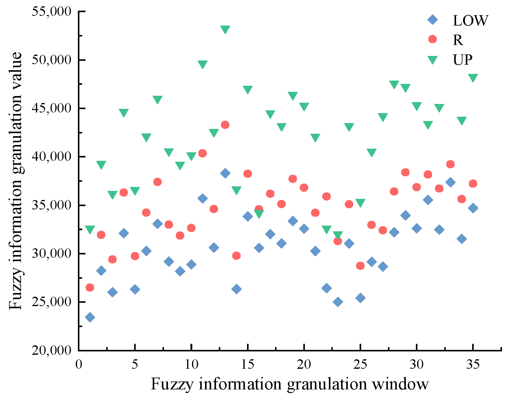
Based on the IC card data of bus passenger flow and the corresponding influencing factors in Harbin from 1 March 2021, to 31 October 2021, covering a total of 245 days, fuzzy granulation was performed with periods of 3, 5, 7, and 14 days according to the results of the passenger flow fluctuation characteristic analysis. The three sets of granulated window data—the minimum value (LOW), mean value (R), and maximum value (UP)—were extracted to represent the fluctuation trends and spatial range indicators of bus passenger flow, and were then used as the inputs of the IWOA-BiGRU model. The corresponding prediction results are presented in

Table 9. Prediction results of IWOA-BiGRU with fuzzy granulated input windows.

Period	LOW			R			UP
	MAE	RMSE	MAPE	MAE	RMSE	MAPE	MAE	RMSE	MAPE
3d	2983	3360	10.0	3256	3652	11.0	4729	5045	11.6
5d	2883	3248	9.7	3068	3435	10.3	4562	4865	11.2
7d	2376	2555	7.8	2804	2941	8.1	3565	3730	8.5
14d	2654	2915	8.9	2876	3230	9.6	3926	4115	10.1

.

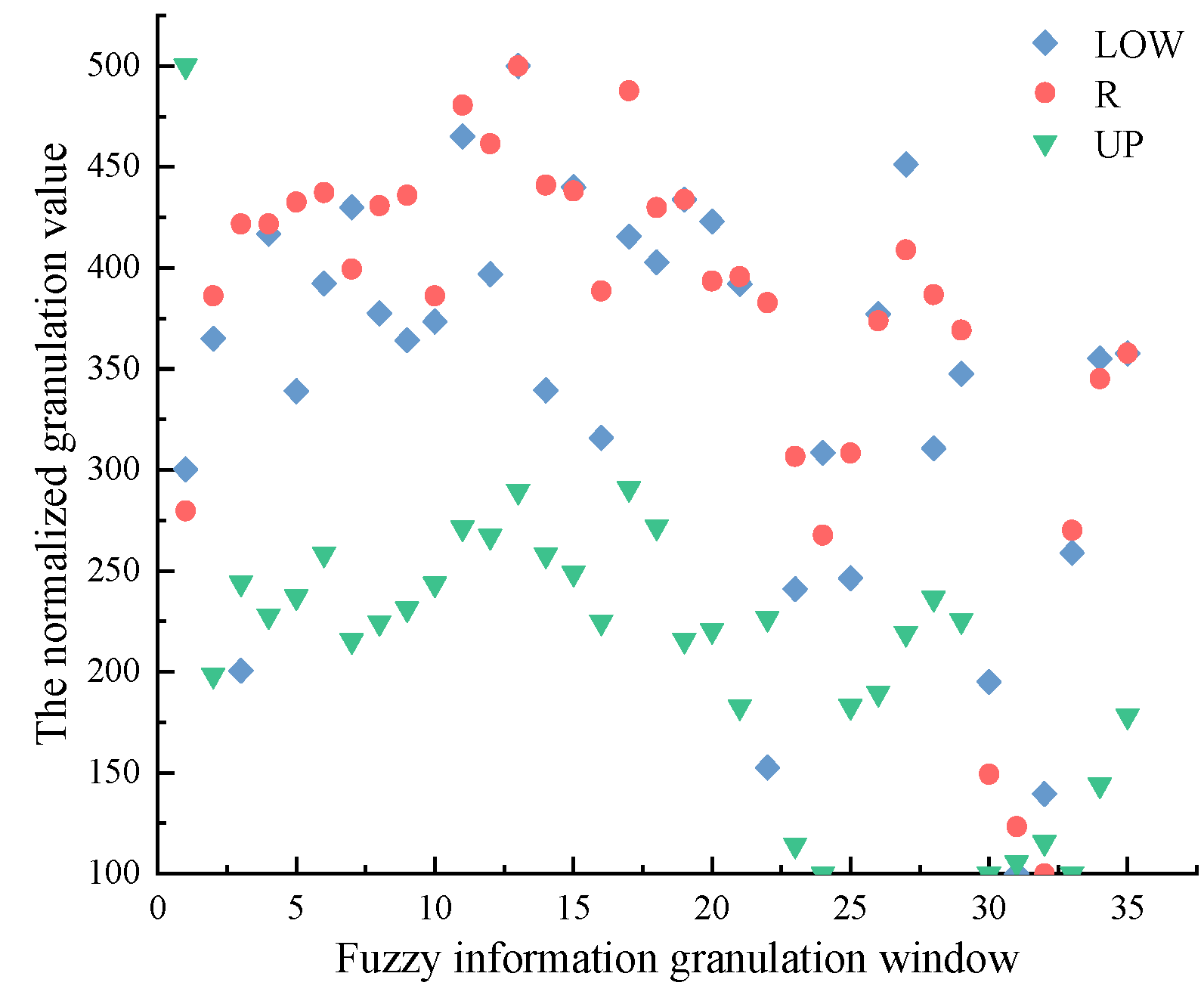
As shown in Table 9, when applying a 7-day weekly cycle for fuzzy granulation, the 245 days of bus passenger flow data are divided into 35 fuzzy granulated windows, which achieves superior prediction accuracy. This is mainly because the division method not only accounts for the travel cycles of working days and non-working days of domestic residents but also ensures a sufficient sample size after partitioning. Using triangular fuzzy membership functions for fuzzy granulation processing, the minimum value (LOW), mean value (R), and maximum value (UP) were obtained to represent the fluctuation trends and spatial range indicators of bus passenger flow. The specific results are shown in Figure 9, and the normalized data within the interval (0,1) are shown in Figure 10.

5.4.2. Forecasting Results Analysis

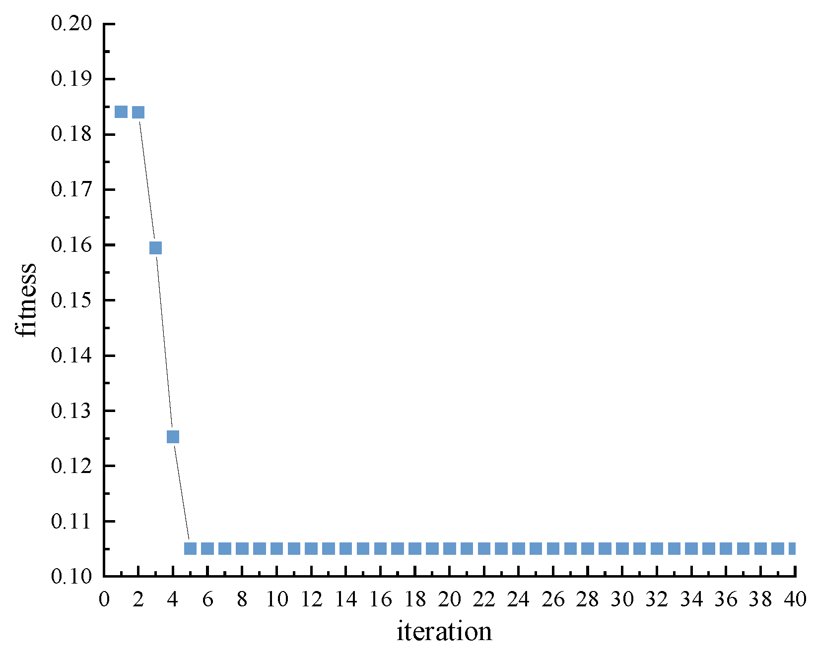
After dividing the bus passenger flow data into fuzzy granulation windows with a 7-day length, 35 sets of new window data were obtained. The data from weeks 1–17 were used as the training set to establish the predictive regression function of the model, while the data from weeks 18–35 were used as the testing set to verify the model’s effectiveness. The parameter settings of the IWOA were as follows: population size POP = 25, maximum number of iterations Max_iter = 40, lower bounds of variable values lb = [0.0001,10,0.00001], upper bounds of variable values ub = [0.01,100,0.005], and variable dimension dim = length(lb).

The fuzzy-granulated bus passenger flow data of LOW, R, and UP were used as the inputs of the IWOA-BiGRU. The IWOA was employed to optimize the parameters of the regression prediction model, and the fuzzy-granulated prediction values of bus passenger flow were obtained. The fitness variation in the fuzzy-granulated bus passenger flow data fitted regression function is shown in Figure 11. To evaluate the accuracy of the forecasting results, regression analysis was conducted to examine the linear correlation between the actual and predicted values, as shown in Figure 12. From Figure 12, it can be observed that the actual and predicted values of the three fuzzy-granulated data groups (LOW, R, and UP) exhibit strong linear correlations. The slopes are 0.8699, 0.7507, and 0.9146, and the correlation coefficients $R^2$ are 0.9058, 0.9119, and 0.9146, respectively. This indicates that the differences between the actual and predicted values are small, and the regression model achieves good prediction accuracy.

5.5. Analysis of Model Parameter Impacts

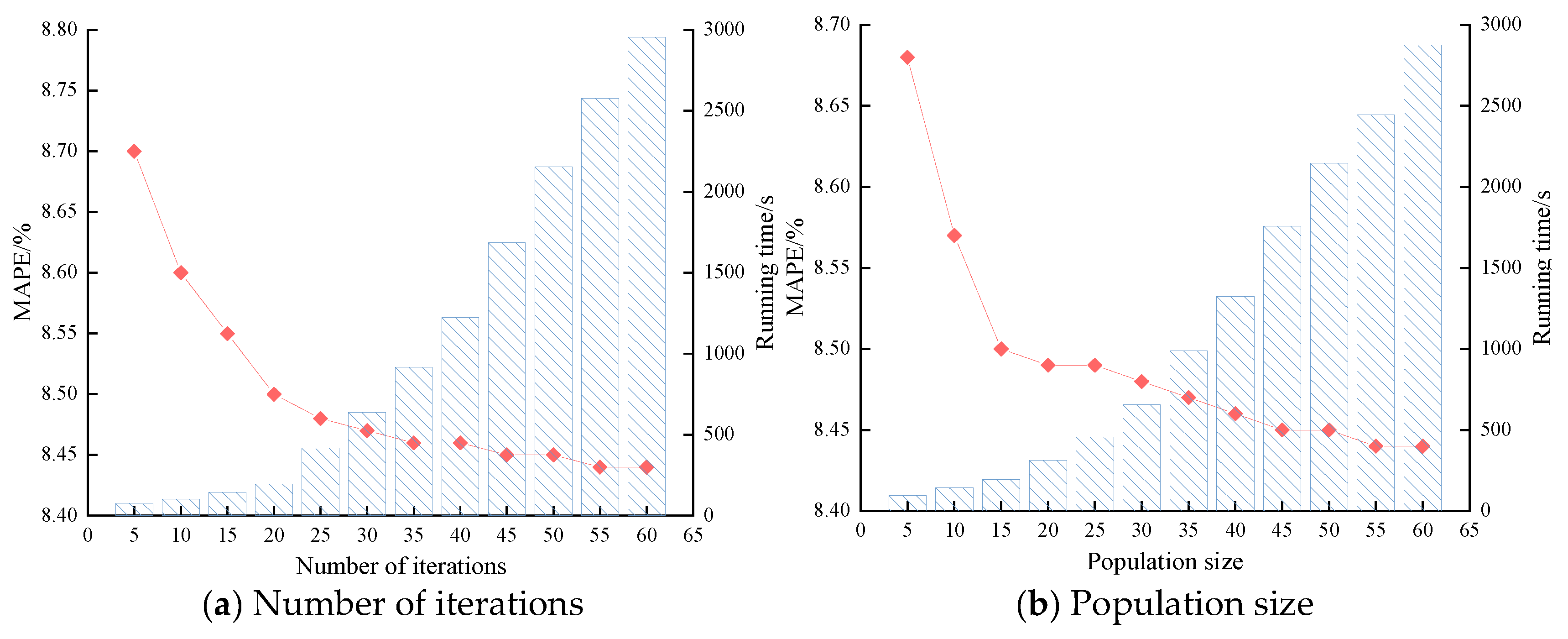
The maximum number of iterations in the bus passenger flow fluctuation trend and spatial prediction model refers to the number of times, after determining the optimal sample position, that other samples update their positions toward the optimal one in order to obtain the global optimum under the IWOA according to dataset characteristics. Due to space limitations, the parameter impact analysis was performed only on the R data after fuzzy granulation of bus passenger flow. Based on the parameter settings of the bus passenger flow fluctuation trend and spatial prediction model, the maximum number of iterations was set to 5, 10, 15, …, 60. The corresponding MAPE values of the prediction results are shown in Figure 13a. As seen in Figure 13a, with other IWOA parameters fixed, when the maximum number of iterations exceeds 40, the growth ratio of MAPE values relative to the number of iterations decreases significantly, while the computation time of the model increases notably. Excessive iteration settings may lead to redundant calculations on sample data, thereby prolonging the runtime of the prediction model.

The population size in the bus passenger flow fluctuation trend and spatial prediction model represents the exploration space of the IWOA during each run. A larger exploration space increases the probability of finding the optimal individual and the global optimum. Based on the parameter settings of the prediction model for R data after fuzzy granulation of bus passenger flow, the population size was set to 5, 10, 15, …, 60. The corresponding MAPE values of the prediction results are shown in Figure 13b. As observed in Figure 13b, when the population size exceeds 25, the growth ratio of MAPE values relative to the number of iterations decreases significantly, but the model runtime increases considerably. An excessively large population size may result in an overly wide search space, leading to redundant feature information and prolonged runtime of the prediction model.

5.6. Comparative Analysis of Model Forecasting Results

To further compare the prediction results of the models, the population size of IWOA, WOA, PSO, and GA was uniformly set to 25, with a maximum iteration number of 40, and the BiGRU algorithm parameters were kept consistent. The three sets of window data—LOW, R, and UP—obtained after fuzzy granulation of bus passenger flow were used as the input for both the IWOA-BiGRU model and existing forecasting models, and the corresponding prediction results were obtained. The statistical errors of the forecasting results for each model are shown in Figure 14. As illustrated in Figure 14, the error statistics of the IWOA-BiGRU model are consistently lower than those of the existing forecasting models. It is noteworthy that the forecasting error of bus passenger flow fuzzy granulation results is inversely proportional to the granulation values. The main reason may be that as the granulation values increase, the fluctuation trends and spatial variation ranges of the fuzzy-granulated bus passenger flow data become relatively larger.

According to

Table 10. Comparison of bus passenger flow forecast results.

Category	LOW			R			UP
	MAE	RMSE	MAPE	MAE	RMSE	MAPE	MAE	RMSE	MAPE
IWOA-BiGRU	2376	2555	7.8	2804	2941	8.1	3565	3730	8.5
WOA-BiGRU	2710	3003	9.1	3296	3743	9.6	4190	4537	10.2
Transformer	2917	3240	9.8	3536	3955	10.0	4502	4826	11.0
PSO-LSSVM	3123	3481	10.5	3925	4333	11.1	5119	5284	11.9
GA-BP	3229	3645	10.9	4089	4346	11.6	5330	5558	12.4
BiGRU	3349	3717	11.3	4155	4400	11.8	5375	5602	12.5

, the average MAE, RMSE, and MAPE of the IWOA-BiGRU forecasting results for the three groups of window data (LOW, R, and UP) after bus passenger flow fuzzy granulation are 2915, 3075, and 8.1%, respectively. Compared with WOA-BiGRU, the improvements are 484, 686, and 1.5%; compared with PSO-LSSVM, the improvements are 1141, 1291, and 3.0%; compared with GA-BP, the improvements are 1301, 1441, and 3.5%; and compared with BiGRU, the improvements are 1378, 1498, and 3.7%. Meanwhile, relative to the existing Transformer algorithm, the improvements are 737, 932, and 2.1%, respectively. It is noteworthy that the MAPE of all models is positively correlated with the granulation values, but the variation in IWOA-BiGRU is the smallest, indicating better robustness and applicability.

To further compare and analyze the performance of the IWOA-BiGRU prediction results, the mean MAPE values of the three window sets (LOW, R, and UP) predicted by the IWOA-BiGRU model were subjected to paired t-tests with the corresponding mean MAPE values predicted by WOA-BiGRU, Transformer, PSO-LSSVM, GA-BP, and BiGRU, denoted as T1, T2, T3, T4, and T5, respectively. The results of the paired t-tests for the mean MAPE values of the prediction results of each model are presented in

Table 11. Paired t-test results of mean MAPE for each model.

Category	Paired Differences					T	Df	Sig. (2-Tailed)
	Mean	Std. Deviation	Std. Error Mean	95% Confidence Interval Lower Bound	95% Confidence Interval Lower Bound
T1	−1.490	3.785	0.892	−3.372	0.392	−1.671	17	0.046
T2	−2.122	4.347	1.025	−4.283	0.040	−2.071	17	0.032
T3	−3.029	3.478	0.820	−4.758	−1.299	−3.694	17	0.002
T4	−3.496	3.405	0.803	−5.189	−1.80	−4.356	17	0
T5	−3.730	3.286	0.775	−5.365	−2.096	−4.816	17	0

. As shown in Table 11, the significance levels of the mean MAPE values predicted by the IWOA-BiGRU model are all less than 0.05, indicating that the IWOA-BiGRU model demonstrates significant superiority in predicting bus passenger flow fluctuations.

As shown in

Table 12. Fluctuation trend and spatial prediction of bus passenger flow.

Category	Time Series							Fluctuation Trend and Space
Date	18	19	20	21	22	23	24	Actual variation range (fuzzy example description)
Actual Passenger Flow	38,638	40,586	42,855	32,053	31,814	36,541	32,650	[Low, R, UP] = [31,527, 35,625, 43,822]
Date	25	26	27	28	29	30	31	Predicted variation range (fuzzy example description)
Actual Passenger Flow	34,620	39,539	46,912	48,846	50,646	36,712	41,715	[Low, R, UP] = [34,539, 39,447, 51,224]

, the upper and lower bounds of the bus passenger flow data thresholds obtained through triangular fuzzy information granulation encompass the range of the actual passenger flow data. From Figure 11 and Figure 13, combined with the data in Table 8 and Table 9, it can be seen that the IWOA-BiGRU forecasting results for the fuzzy-granulated bus passenger flow data (LOW, R, and UP) in week 35 (25–31 October 2021) are 34,539, 39,447, and 51,224, respectively. The prediction accuracy of this model is higher compared with existing forecasting models. Relative to the fuzzy-granulated values of bus passenger flow in the previous week (31,527, 35,625, and 43,822), the model forecasting results show an overall upward trend, which is generally consistent with the actual data trend, indicating the reliability of the forecasting results.

These findings provide data support and decision-making references for the formulation of bus operation scheduling plans and for passengers to reasonably plan travel routes and times, demonstrating practical application value.

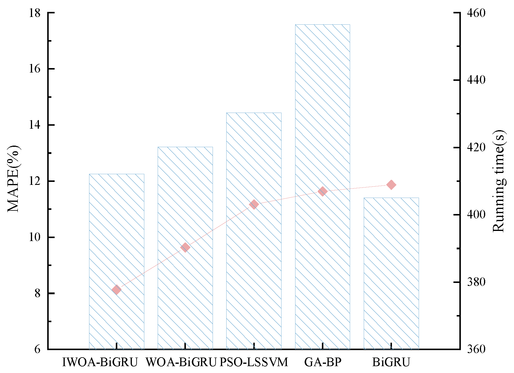
To evaluate the applicability of the IWOA-BiGRU, the average runtime of forecasting models with different fuzzy-granulated bus passenger flow windows was recorded, as shown in Figure 15.

From Figure 15, it can be seen that the average runtime of IWOA-BiGRU is 412 s, which is shorter than that of WOA-BiGRU, PSO-LSSVM, and GA-BP by 8.2 s, 18.3 s, and 44.5 s, respectively. Although its runtime is longer than that of BiGRU, the higher prediction accuracy of IWOA-BiGRU demonstrates better applicability.

6. Conclusions

The main conclusions of this study are as follows:

(1) This paper applies a fuzzy information granulation method, which reduces the spatiotemporal complexity of bus passenger flow data while preserving its valid information, and constructs a FIG-IWOA-BiGRU-based model for forecasting bus passenger flow fluctuation trends and spatial distribution. The MAPE values of the forecasting results for the fuzzy-granulated LOW, R, and UP window data are 7.8%, 8.1%, and 8.5%, respectively. Compared with existing forecasting models, these values improve by 1.3–3.5%, 1.5–3.7%, and 1.7–4.0%, demonstrating good prediction accuracy and robustness. The findings contribute to the reasonable prediction of bus passenger flow fluctuation trends and spatial patterns, providing data support and decision-making references for bus operation scheduling plans and for passengers in planning travel routes and times.

(2) This paper improves the whale optimization algorithm (WOA) with hybrid strategies, including Logistic–Tent combined chaotic mapping, an elite opposition-based learning and Cauchy mutation hybrid mechanism, and modified convergence factor and inertia weight. These strategies enhance population diversity and quality while preserving the strengths of WOA, and improve the algorithm’s capability to balance global search and local exploitation. Comparative analysis of numerical simulation results and convergence characteristics on 21 benchmark test functions shows that IWOA outperforms WOA, GWO, PSO, and GA in solution accuracy, convergence speed, and the ability to escape local optima, further validating the effectiveness of the hybrid strategy-improved WOA proposed in this study.

In addition, due to the privacy of bus data, this study did not obtain operational data from other cities, which imposes certain limitations. In future research, the following aspects will be further explored:

(1) The main research content of this study is based on Harbin city’s bus IC card and weather condition data. Future research should further collect and organize bus IC card and weather data from other cities to comparatively analyze the impact of different built environments on the spatiotemporal distribution, fluctuation characteristics, and trends of bus passenger flow.

(2) Based on the analysis of bus passenger flow data in different urban regions, by considering modifications to the whale optimization algorithm’s search mechanism and algorithm structure and integrating the advantages of other intelligent optimization algorithms, more efficient intelligent optimization algorithms with improved search and convergence speed can be proposed, thereby enhancing the accuracy and applicability of models predicting bus passenger flow fluctuation trends and spatial distribution.

References

1. Mei, Z.; Yu, W.; Tang, W.; Yu, J.; Cai, Z. Attention mechanism-based model for short-term bus traffic passenger volume prediction. IET Intell. Transp. Syst. 2023, 17, 767–779. [Google Scholar] [CrossRef]
2. Chen, D.; Kun, Y.; Chun, G. The Relationship between Built Environment Characteristics and Metro Stations Pedestrian Catchment Areas. J. Adv. Transp. 2024, 2024, 2196799. [Google Scholar] [CrossRef]
3. Zhu, C.; Sun, X.; Li, Y.; Wang, Z.; Li, Y. A hybrid neural network for urban rail transit short-term flow prediction. J. Supercomput. 2024, 80, 24297–24323. [Google Scholar] [CrossRef]
4. Fang, X.; Lin, M.; Chen, W.; Pan, X. Forecasting short-term passenger flow on a bus route: A splitting-integrating method based on passenger travel behavior. Transport 2025, 40, 12–23. [Google Scholar] [CrossRef]
5. Chen, E.; Ye, Z.; Wang, C.; Xu, M. Subway passenger flow prediction for special events using smart card data. IEEE Trans. Intell. Transp. Syst. 2019, 21, 1109–1120. [Google Scholar] [CrossRef]
6. Milenković, M.; Švadlenka, L.; Melichar, V.; Bojović, N.; Avramović, Z. SARIMA modelling approach for railway passenger flow forecasting. Transport 2018, 33, 1113–1120. [Google Scholar] [CrossRef]
7. Cheng, G.; He, C. Analysis of bus travel characteristics and predictions of elderly passenger flow based on smart card data. Electron. Res. Arch. 2022, 30, 4256–4276. [Google Scholar] [CrossRef]
8. Wang, J.; Leng, B.; Wu, J.; Du, H.; Xiong, Z. Metroeye: A weather-aware system for real-time metro passenger flow prediction. IEEE Access 2020, 8, 129813–129829. [Google Scholar] [CrossRef]
9. Yu, L.; Cui, M.; Dai, S. Deviation of peak hours for metro stations based on least square support vector machine. PLoS ONE 2023, 18, e0291497. [Google Scholar] [CrossRef]
10. Xu, X.; Zhang, K.; Mi, Z.; Wang, X. Short-term passenger flow prediction during station closures in subway systems. Expert Syst. Appl. 2024, 236, 121362. [Google Scholar] [CrossRef]
11. Li, Y.; Ma, C. Short-time bus route passenger flow prediction based on a secondary decomposition integration method. J. Transp. Eng. Part A Syst. 2023, 149, 04022132. [Google Scholar] [CrossRef]
12. Yazıcıoğlu, C.; Akgüngör, A.P. Modeling Short-Term Passenger Flows in Metro and Bus Systems Using Meteorological Data: Deep Learning Model Comparisons. Appl. Sci. 2025, 15, 6260. [Google Scholar] [CrossRef]
13. Zhang, Y.; Wang, X.; Xie, J.; Bai, Y. Comparative analysis of deep-learning-based models for hourly bus passenger flow forecasting. Transportation 2024, 51, 1759–1784. [Google Scholar] [CrossRef]
14. Cao, B.; Li, Y.; Chen, Y.; Yang, A. A CNN-LSTM model for short-term passenger flow forecast considering the built environment in urban rail transit stations. J. Transp. Eng. Part A Syst. 2024, 150, 04024072. [Google Scholar] [CrossRef]
15. Baghbani, A.; Rahmani, S.; Bouguila, N.; Patterson, Z. TMS-GNN: Traffic-aware Multistep Graph Neural Network for bus passenger flow prediction. Transp. Res. Part C Emerg. Technol. 2025, 174, 105107. [Google Scholar] [CrossRef]
16. Lv, W.; Lv, Y.; Ouyang, Q.; Ren, Y. A bus passenger flow prediction model fused with point-of-interest data based on extreme gradient boosting. Appl. Sci. 2022, 12, 940. [Google Scholar] [CrossRef]
17. Yu, J.; Chang, X.; Hu, S.; Yin, H.; Wu, J. Combining travel behavior in metro passenger flow prediction: A smart explainable Stacking-Catboost algorithm. Inf. Process. Manag. 2024, 61, 103733. [Google Scholar] [CrossRef]
18. Nagaraj, N.; Gururaj, H.L.; Swathi, B.H.; Hu, Y.C. Passenger flow prediction in bus transportation system using deep learning. Multimed. Tools Appl. 2022, 81, 12519–12542. [Google Scholar] [CrossRef]
19. Sun, F.; Wang, X.L.; Zhang, Y.; Liu, W.X.; Zhang, R.J. Analysis of bus trip characteristic analysis and demand forecasting based on GA-NARX neural network model. IEEE Access 2020, 8, 8812–8820. [Google Scholar] [CrossRef]
20. Li, C.; Wang, X.; Cheng, Z.; Bai, Y. Forecasting bus passenger flows by using a clustering-based support vector regression approach. IEEE Access 2020, 8, 19717–19725. [Google Scholar] [CrossRef]
21. Sivakumar, R.; Angayarkanni, S.A.; Ramana Rao, Y.V. Traffic flow forecasting using natural selection based hybrid Bald Eagle Search—Grey Wolf optimization algorithm. PLoS ONE 2022, 17, e0275104. [Google Scholar] [CrossRef]
22. Jiang, Q. GMM Clustering Based on WOA Optimization and Space-Time Coupled Urban Rail Traffic Flow Prediction by CEEMD-SE-BiGRU-AM. Mob. Inf. Syst. 2022, 2022, 7846630. [Google Scholar] [CrossRef]
23. Rana, N.; Latiff, M.S.A.; Abdulhamid, S.M.; Chiroma, H. Whale optimization algorithm: A systematic review of contemporary applications, modifications and developments. Neural Comput. Appl. 2020, 32, 16245–16277. [Google Scholar] [CrossRef]
24. Xu, Y.; Li, Q.; Xu, X.; Yang, J.; Chen, Y. Research progress of nature-inspired metaheuristic algorithms in mobile robot path planning. Electronics 2023, 12, 3263. [Google Scholar] [CrossRef]
25. Nadimi-Shahraki, M.H.; Zamani, H.; Asghari Varzaneh, Z.; Mirjalili, S. A systematic review of the whale optimization algorithm: Theoretical foundation, improvements, and hybridizations. Arch. Comput. Methods Eng. 2023, 30, 4113–4159. [Google Scholar] [CrossRef]
26. Prasad, D.; Mukherjee, A.; Mukherjee, V. Temperature dependent optimal power flow using chaotic whale optimization algorithm. Expert Syst. 2021, 38, e12685. [Google Scholar] [CrossRef]
27. Duan, Y.; Liu, C.; Li, S. Battlefield target grouping by a hybridization of an improved whale optimization algorithm and affinity propagation. IEEE Access 2021, 9, 46448–46461. [Google Scholar] [CrossRef]
28. Darvish Falehi, A. An optimal second-order sliding mode based inter-area oscillation suppressor using chaotic whale optimization algorithm for doubly fed induction generator. Int. J. Numer. Model. Electron. Netw. Devices Fields 2022, 35, e2963. [Google Scholar] [CrossRef]
29. Paul, C.; Roy, P.K.; Mukherjee, V. Wind and Solar Based Multi-Objective Hydro-Thermal Scheduling Using Chaotic-Oppositional Whale Optimization Algorithm. Electr. Power Compon. Syst. 2023, 51, 568–592. [Google Scholar] [CrossRef]
30. Li, M.; Yu, X.; Fu, B.; Wang, X. A modified whale optimization algorithm with multi-strategy mechanism for global optimization problems. Neural Comput. Appl. 2023, 2023, 22339–22352. [Google Scholar] [CrossRef]
31. Chakraborty, S.; Saha, A.K.; Chhabra, A. Improving Whale Optimization Algorithm with Elite Strategy and Its Application to Engineering-Design and Cloud Task Scheduling Problems. Cogn. Comput. 2023, 15, 1497–1525. [Google Scholar] [CrossRef]
32. Anitha, J.; Pandian, S.I.A.; Agnes, S.A. An efficient multilevel color image thresholding based on modified whale optimization algorithm. Expert Syst. Appl. 2021, 178, 115003. [Google Scholar] [CrossRef]
33. Yue, Y.; You, H.; Wang, S.; Cao, L. Improved whale optimization algorithm and its application in heterogeneous wireless sensor networks. Int. J. Distrib. Sens. Netw. 2021, 17, 15501477211018140. [Google Scholar] [CrossRef]
34. Chakraborty, S.; Saha, A.K.; Nama, S.; Debnath, S. COVID-19 X-ray image segmentation by modified whale optimization algorithm with population reduction. Comput. Biol. Med. 2021, 139, 104984. [Google Scholar] [CrossRef] [PubMed]
35. Wang, H.; Wu, F.; Zhang, L. Application of variational mode decomposition optimized with improved whale optimization algorithm in bearing failure diagnosis. Alex. Eng. J. 2021, 60, 4689–4699. [Google Scholar] [CrossRef]
36. Yang, W.; Xia, K.; Fan, S.; Wang, L.; Li, T.; Zhang, J.; Feng, Y. A multi-strategy Whale optimization algorithm and its application. Eng. Appl. Artif. Intell. 2022, 108, 104558. [Google Scholar] [CrossRef]
37. Ju, C.; Ding, H.; Hu, B. A hybrid strategy improved whale optimization algorithm for web service composition. Comput. J. 2023, 66, 662–677. [Google Scholar] [CrossRef]
38. Liu, J.; He, Q.; Yue, Z.; Pei, Y. A Hybrid Strategy-Improved SSA-CNN-LSTM Model for Metro Passenger Flow Forecasting. Mathematics 2024, 12, 3929. [Google Scholar] [CrossRef]
39. Mirjalili, S.; Lewis, A. The whale optimization algorithm. Adv. Eng. Softw. 2016, 95, 51–67. [Google Scholar] [CrossRef]
40. Kaur, G.; Arora, S. Chaotic whale optimization algorithm. J. Comput. Des. Eng. 2018, 5, 275–284. [Google Scholar] [CrossRef]
Figure 1. Travel characteristics of bus passenger flow.
Mathematics 13 03204 g001
Figure 2. Correlation of influencing factors of bus passenger flow.
Mathematics 13 03204 g002
Figure 3. Histogram distribution of bus passenger flow and fuzzy membership functions.
Mathematics 13 03204 g003
Figure 4. Structure of BiGRU.
Mathematics 13 03204 g004
Figure 5. Flowchart of Bus Passenger Flow Fluctuation Trend and Spatial Prediction Based on FIG-IWOA-BiGRU.
Mathematics 13 03204 g005
Figure 6. Benchmark function box line statistics.
Mathematics 13 03204 g006aMathematics 13 03204 g006b
Figure 7. Average convergence curves of benchmark test functions.
Mathematics 13 03204 g007aMathematics 13 03204 g007b
Figure 8. Algorithm runtime comparison.
Mathematics 13 03204 g008
Figure 9. Visualization of fuzzy information granulation.
Mathematics 13 03204 g009
Figure 10. Normalized granulation values.
Mathematics 13 03204 g010
Figure 11. Fitness variation.
Mathematics 13 03204 g011
Figure 12. Correlation between actual and predicted values under different bus passenger flow fluctuation trends (LOW/R/UP).
Mathematics 13 03204 g012
Figure 13. Impacts of model parameters on forecasting results.
Mathematics 13 03204 g013
Figure 14. Error comparison analysis under different bus passenger flow fluctuation trends (LOW/R/UP).
Mathematics 13 03204 g014
Figure 15. Average runtime of different models.
Mathematics 13 03204 g015