Interval-Valued Multi-Step-Ahead Forecasting of Green Electricity Supply Using Augmented Features and Deep-Learning Algorithms

Abstract

Accurately forecasting the interval-valued green electricity (GE) supply is challenging due to the unpredictable and instantaneous nature of its source; yet, reliable multi-step-ahead forecasting is essential for providing the lead time required in operations, resource allocation, and system management. This study proposes an augmented-feature multi-step interval-valued forecasting (AFMIF) scheme that aims to address the challenges in forecasting interval-valued GE supply data by extracting additional features hidden within an interval. Unlike conventional methods that rely solely on original interval bounds, AFMIF integrates augmented features that capture statistical and dynamic properties to reveal hidden patterns. These features include basic interval boundaries and statistical distributions from an interval. Three effective forecasting methods, based on gated recurrent units (GRUs), long short-term memory (LSTM), and a temporal convolutional network (TCN), are constructed under the proposed AFMIF scheme, while the mean ratio of exclusive-or (MRXOR) is used to evaluate the forecasting performance. Two different real datasets of wind-based GE supply data from Belgium and Germany are used as illustrative examples. Empirical results demonstrate that the proposed AFMIF scheme with GRUs can generate promising results, achieving a mean MRXOR of 0.7906 from the Belgium data and 0.9719 from the Germany data for one-step- to three-steps-ahead forecasting. Moreover, the TCN yields an average improvement of 13% across all time steps with the proposed scheme. The results highlight the potential of the AFMIF scheme as an effective alternative approach for accurate multi-step-ahead interval-valued GE supply forecasting that offers practical benefits supporting GE management.

1. Introduction

With the rapid increase in electricity demand and concerns over greenhouse gas emissions from fossil fuels [1,2,3,4], renewable energy has become a vital alternative for sustainable electricity generation [5,6,7]. However, sources such as wind and solar are inherently variable and unpredictable, creating challenges in ensuring a stable and reliable electricity supply [7,8]. This variability makes the accurate forecasting of green electricity (GE) generation essential for effective operation and planning [9,10]. Given the essential characteristic of the natural resources used for GE generation, the daily actual production output is often unstable, exhibiting a wide range of interval values, which can be represented as interval-valued GE supply data [11]. Interval-valued GE supply data represent GE production records over a day, captured at specific recording intervals (e.g., 15 min per record). This characteristic presents significant challenges for GE supply management. Consequently, the effective forecasting of interval-valued GE supply data is a crucial area of investigation [12,13,14]. For example, the potential maximum and minimum electricity production can be estimated when forecasting the interval values of GE supply. This information is crucial for power-grid managers to monitor the GE supply and to make informed decisions [14,15]. Consequently, given the inherent complexity of GE data, the development of effective forecasting models and the delivery of useful information to support decision-making are valuable.

Interval-valued forecasting is an important topic in studies concerning GE supply [16,17]. For example, Gupta et al. [18] forecasted interval-valued wind power supply data by combining wavelet and autoregressive integrated moving average (ARIMA) models. Wang et al. [19] employed a multi-objective feature extraction approach to reconstruct decomposed interval-valued wind power data during forecasting. Yang et al. [20] proposed an ensemble-based forecasting system for interval-valued wind power supply data.

However, most existing studies have paid limited attention to multi-step-ahead forecasting for interval-valued GE data [18,19,20], with those that have often focusing on point forecasts [21,22]. To illustrate, Yu et al. [23] combined convolution layers and long short-term memory (LSTM) for forecasting wind speed 10 min ahead. Nguyen et al. [24] utilized stacked temporal convolutional networks (TCNs) to forecast wind power output values from one to six steps ahead, with each step length being 30 min-based. Tsegaye et al. [25] forecasted power loads with hour- and day-based step lengths using LSTM with population-based adaptive optimization. Given the inherently uncertain nature of GE data, one-step-ahead forecasting provides limited information [16]. For instance, preparing a GE supply often requires lead time for scheduling, coordination, and resource allocation [26]. However, one-step-ahead forecasting offers a narrow window of information for action, providing limited flexibility to plan schedules or manage unexpected fluctuations [12]. In contrast, multi-step-ahead forecasting extends the forecasting horizon, generating more future information that extends the buffer time during operation. This enables managers to gain more informed insights regarding the expected range of the GE supply over longer future horizons, supporting more effective planning such as maintenance or resource allocation [12,16]. Therefore, the accurate multi-step-ahead forecasting of the interval-valued GE supply can benefit GE management.

Furthermore, when forecasting interval-valued GE supply data, the targets are typically represented in either the upper and lower bound or center and radius formats [14]. Either format can express the upper and lower bounds of an interval-valued data point. Most existing studies on forecasting interval-valued GE supply data have primarily considered basic features, such as the time-lagged information of the target variable, as predictor variables directly derived from upper and lower bounds or central and radius data [14]. However, these basic features fail to capture other useful information for the forecasting task, such as the distribution information within an interval-valued data point [27,28,29]. This information can be described using augmented features such as the quartile values, mean, interquartile range (IQR), skewness, and kurtosis. These augmented features can capture inherent information from an interval-valued data point and can be incorporated into the forecasting model to enhance the forecasting performance. Few studies have considered augmented features when forecasting interval-valued GE supply data. Jiang et al. [27] demonstrated the potential of utilizing augmented features, but they only considered the quartile values, minimum value, and maximum value for the one-step-ahead forecasting of the regular electricity demand, and not GE supply data. Chang et al. [28] took a similar approach and added the mean, IQR, skewness, and kurtosis as additional augmented features for the one-step-ahead forecasting of the regular electricity supply. However, to the best of our knowledge, no study has simultaneously considered both augmented feature usage and multi-step-ahead forecasting for interval-valued GE supply data. Therefore, addressing this research gap warrants further investigation.

Various methods are utilized for the interval-valued forecasting of GE supply data, including seasonal ARIMA (SARIMA) and deep-learning (DL) algorithms [10,30]. Because interval-valued forecasting involves a pair of target variables (upper and lower bounds or central and radius), it is considered a multi-output task that DL models can handle effectively and conveniently. For example, Niu et al. [31] proposed a framework combining LSTM networks with several decomposition methods to achieve high performance in wind power interval-valued forecasting. Zhou et al. [32] forecasted wind power intervals using LSTM. Wang et al. [33] proposed a framework using a modified scaling approach and efficient feature ranking to improve the performance of gated recurrent unit (GRU) networks in wind power interval-valued forecasting. Wang et al. [34] forecasted wind power intervals with a modified GRU combining two layers of decomposition methods. TCNs have also been used in interval-valued forecasting studies [35,36]. Hu et al. [35] proposed and applied a slightly modified TCN algorithm for wind power interval forecasting, whereas Gan et al. [36] added an adaptive layer to the TCN layer to predict wind speed intervals. Therefore, as interval-valued forecasting is a multi-output task, the commonly used LSTM, GRU, and TCN models are employed in this study.

This study proposes a multi-step-ahead forecasting scheme that incorporate augmented features (base and distribution features) and DL models (GRU, LSTM, and TCN) to forecast the interval-valued GE supply effectively. The proposed scheme is named the Augmented Feature Multi-Step Interval-valued Forecasting (AFMIF) scheme and consists of four steps. First, interval-valued data are generated by preprocessing the original GE supply data, which are records of daily electricity logs within a given time cycle. Second, augmented features are constructed from the interval-valued data that are represented in the upper and lower bound and central and radius formats. Third, LSTM, GRU, and TCN models are constructed, incorporating the augmented and basic features of the interval-valued data, to create three multi-step-ahead interval-valued forecasting models, namely, AFMIF-GRU, AFMIF-LSTM, and AFMIF-TCN, respectively. Finally, these three forecasting models are compared with four other models to evaluate the performance of the proposed AFMIF scheme, and the best model is selected. SARIMA is one of the comparison models used as the benchmark method as it is a commonly used method in GE data forecasting. The mean ratio of exclusive-or (MRXOR) is used to assess the overlap between the actual and estimated intervals. Wind power is a key source of GE and has gained global popularity, with a rapid annual growth rate of 12.6% in wind turbine installations in recent years [9,37,38,39]. Thus, this study uses wind-power-based GE supply data from Belgium and Germany as illustrative examples to evaluate the performance of the proposed AFMIF scheme.

Table 1. Overview of this study compared to existing literatures.

Study	Forecasting Models	Feature Usage	Time-Step	Target
This study	AFMIF incorporates GRU, LSTM, and TCN	Basic and augmented (quartile, minimum, maximum, IQR, mean, kurtosis, and skewness values)	Multi-step	Interval-valued
Jiang et al. [27]	Support vector regression	Basic and augmented (quartile, minimum, and maximum values)	One-step	Interval-valued
Chang et al. [28]	Multivariate adaptive regression splines	Basic and augmented (quartile, minimum, maximum, IQR, mean, kurtosis, and skewness values)
Gupta et al. [18]	ARIMA incorporates Wavelet	Basic
Wang et al. [19]	Feature extraction and decomposition method	Basic
Yang et al. [20]	Ensemble of DL, ARIMA, and decomposition method	Basic
Wang et al. [33]	Modified scaling and efficient feature ranking improving GRU	Basic
Wang et al. [34]	GRU with decomposition	Basic
Hu et al. [35]	Conformalized-quantile-regression-based TCN	Basic
Tsegaye et al. [25]	Population-based adaptive optimization and LSTM	Basic with external variables	Multi-step	Point forecast
Nahid et al. [21]	LSTM incorporates convolution network with decomposition	Basic
Pavlov-Kagadejev et al. [22]	Metaheuristics-based LSTM with decomposition	Basic
Yu et al. [23]	LSTM incorporates convolution network	Basic
Nguyen et al. [24]	Stacked TCN	Basic

provides a comparative overview of the research gap and highlights the contributions of this study relative to the existing literature.

The remainder of this paper is organized as follows: Section 2 introduces the DL methods and proposed AFMIF scheme. Section 3 presents the processed Belgium and Germany data, descriptive statistics of the augmented features, model results, and robustness evaluation. Finally, Section 4 summarizes the findings.

2. Methodology

This section provides a brief introduction to the LSTM, GRU, and TCN methods, followed by a step-by-step explanation of the proposed AFMIF scheme.

2.1. LSTM

LSTM is an extension of the recurrent neural network that utilizes the concept of retaining information over time to capture long-term dependencies for tasks such as time-series forecasting [40,41]. LSTM retains information via memory cells, each of which is made up of an input gate, a forget gate, and an output gate. The forget gate controls the extent to which previous information should be retained or discarded, and the calculation is shown in Equation (1):

$$f_t=\sigma \left({\mathit{w}}_f·\left[h_{t-1},x_t\right]+b_f\right),$$

(1)

where $t$ is the time period during forecasting; ${\mathit{w}}_f$ is the weight matrix; $h_{t-1}$ is the output of the previous time period; $x_t$ is the input at the current time period; $b_f$ is the bias; and $\mathsf{\sigma }$ is the sigmoid activation function. The input gate regulates the flow of new information into the cell state that determines updating or retaining new information to overwrite previous information. The calculation is expressed as follows:

$$I_t=\sigma \left({\mathit{w}}_I·\left[h_{t-1},x_t\right]+b_I\right),$$

(2)

where $I_t$ yields a value between 0 and 1, where a value closer to 1 means that the information should be updated; ${\mathit{w}}_I$ is the weight matrix; and $b_I$ denotes the bias. Finally, the latest output value $h_t$ is generated through the output gate according to Equations (3) and (4):

$$o_t=\sigma \left({\mathit{w}}_o\left[h_{t-1},x_t\right]+b_o\right)$$

(3)

$$h_t=o_t\times tanh\left(C_t\right),$$

(4)

where ${\mathit{w}}_o$ is the weight matrix; $b_o$ denotes the bias; and $C_t$ is the overwritten information. For further details, please refer to the original study [39].

2.2. GRU

The concept of the GRU is similar to that of LSTM, with several differences in the gate mechanism [42,43]. The GRU is a lightweight modification of LSTM that simplifies the gate mechanism by merging the gates into update and reset gates. The reset gate $r_t$ can be treated as the forget gate of LSTM, with the purpose of controlling the amount of historical information that should be forgotten. The calculation is shown in Equation (5):

$$r_t=\sigma \left({\mathit{w}}_r·\left[h_{t-1},x_t\right]\right),$$

(5)

where ${\mathit{w}}_r$ is the weight matrix; $h_{t-1}$ is the output of the previous time period; $x_t$ is the input of the current time period; and $\mathsf{\sigma }$ is the sigmoid activation function. The update gate $z_t$ determines the amount of historical information to be carried forward to the current time step. The equation for $z_t$ is expressed as follows:

$$z_t=\sigma \left({\mathit{w}}_z·\left[h_{t-1},x_t\right]\right),$$

(6)

where ${\mathit{w}}_r$ is the weight matrix. Finally, the output $h_t$ at the current state of time step $t$ can be determined using Equation (7):

$$h_t=\left(1-z_t\right)\times h_{t-1}+z_t\times {\tilde{h}}_t,$$

(7)

where ${\tilde{h}}_t$ is the potential candidate value with new information to be added at current time step $t$. The GRU mainly manages the retention and retrieval of input information through reset and update gates for forecasting. For further details, please refer to the original study [41].

2.3. TCN

The TCN is a DL architecture designed for sequential data modeling that is commonly used for time-series forecasting tasks [44,45]. The main mechanism of TCN is the combination of dilated convolution, causal convolution, and residual connection. With these components, the predictions at any time step are conditioned solely on past inputs, preserving the temporal order.

Causal convolution ensures temporal causality by restricting predictions at time step $t$ to depend only on earlier time steps. Its receptive field increases linearly with the number of layers, limiting its ability to capture long-range dependencies in sequential data efficiently. The TCN addresses this limitation by incorporating dilated convolution. Dilated convolution is a variation of standard convolution that introduces gaps between consecutive filter elements, allowing the network to expand its receptive field without increasing the number of parameters, which helps the TCN model to capture long-term dependencies more effectively. Hence, the dilated operation of $F$ on element time step $t$ in a time-series sequence $F\left(t\right)$ can be expressed as follows:

$$F\left(t\right)=\left(x\times {}_{\mathrm{d}}f\right)\left(t\right)={\sum }_{i=0}^{k-1}f\left(i\right)·x_{t-d·i},$$

(8)

where $d$ is the dilation rate; $k$ is the filter size; and $x_{t-d·i}$ is the past state from the previous convolution. Moreover, to improve model stability and reduce the vanishing gradient effect, residual blocks are incorporated into the TCN. A residual block consists of stacked dilated causal convolution layers, followed by a rectified linear unit (ReLU), normalization layers, and a dropout layer for regularization.

LSTM, the GRU, and the TCN were selected because they are well-established DL models that have demonstrated strong performance in time-series forecasting tasks. LSTM and the GRU belong to the recurrent neural network family and are effective in capturing both the long- and short-term temporal dynamics that are suitable for modeling the evolving behavior of complex interval-valued GE supply data. The TCN, which is a convolution-based model, offers the advantages of parallel processing and stable gradients, making it well-suited for learning the temporal patterns that are hidden within the interval-valued data. Moreover, as mentioned in the Introduction, interval-valued GE supply forecasting is a multi-output task that involves two target variables. The three selected DL models are more effective for handling multi-output tasks, as traditional models often require separate models to be built for each target variable.

2.4. Proposed AFMIF Scheme

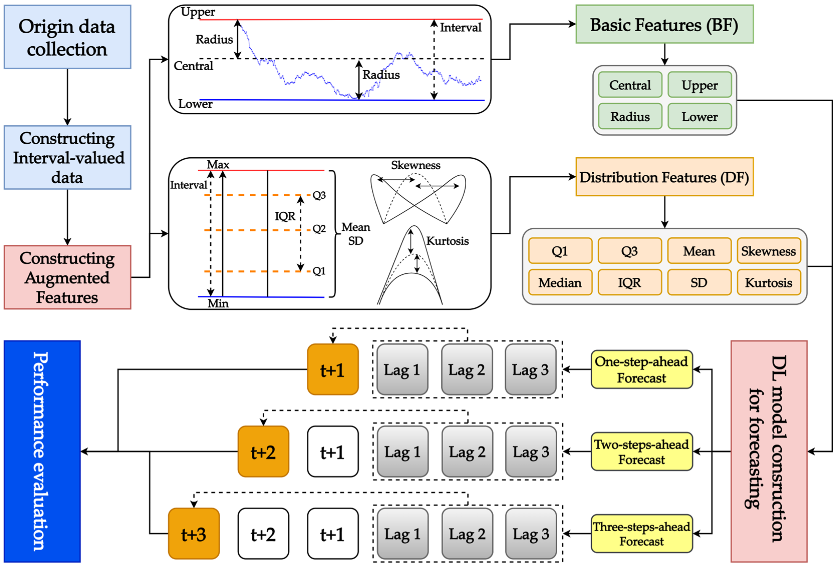
Figure 1 presents the proposed AFMIF scheme.

As shown in the figure, the original data consist of GE data that are generated from wind power, comprising electricity logs recorded at a specified minute-based recording cycle, which are collected first. Subsequently, the collected data are preprocessed to generate interval-valued data using the upper and lower bound and central and radius formats. Once the interval-valued data have been prepared, information can be extracted from them to construct augmented features. Two sets of features are constructed in the AFMIF scheme: the basic feature (BF) consisting of time-lagged information of the upper and lower bounds and central and radius; and the distribution feature (DF) consisting of the Q1, median, Q3, IQR, mean, standard deviation (SD), skewness, and kurtosis. The BF and DF represent different information. The BF is the basic information describing the time-lagged information of the upper bound, lower bound, central, and radius data points of the interval-valued data. The DF considers the time-lagged information of the detailed statistics that are directly extracted from the interval-valued data. After obtaining the predictor variables constituting the BF and DF, three different DL algorithms, namely, LSTM, the GRU, and the TCN, are used to construct models for multi-step-ahead forecasting (i.e., one-step-, two-steps-, and three-steps-ahead) of interval-valued wind power GE supply. As the central and radius format is commonly used in interval-valued forecasting tasks, this study uses this format to form the target variable. Finally, the MRXOR metric is used to evaluate the performance of all constructed models.

The processes of the proposed AFMIF scheme are introduced in the following subsections.

2.4.1. Preprocessing of Interval-Valued Data

The original wind power data systematically represent the electricity produced over time, for which electricity logs are recorded in minute-based cycles per day. Hence, the collected wind power data must first be transformed into interval-valued data. Suppose that a total record ($TR$) of electricity logs ($e$) is recorded each day and $n$ days of data are collected. A matrix ${\mathit{D}}_n$ of size $n$ $\times$ $TR$ can be created and expressed as follows:

$${\mathit{D}}_n=\left[\begin{array}{ccc}{e}_{\mathrm{1,1}}& \dots & e_{1,TR}\\ ⋮& e_{i,j}& ⋮\\ e_{n,1}& \dots & e_{n,TR}\end{array}\right]=\left[\begin{array}{c}{\mathit{d}}_1\\ \begin{array}{c}{\mathit{d}}_2\\ ⋮\\ {\mathit{d}}_n\end{array}\end{array}\right], \mathrm{w}\mathrm{h}\mathrm{e}\mathrm{r}\mathrm{e} i,j\in {\mathit{Z}}^{+},$$

(9)

where ${\mathit{d}}_{\mathit{i}}$(${\mathit{d}}_1,{\mathit{d}}_2,\dots ,{\mathit{d}}_n$) are vectors of the recorded $e$ logs per day.

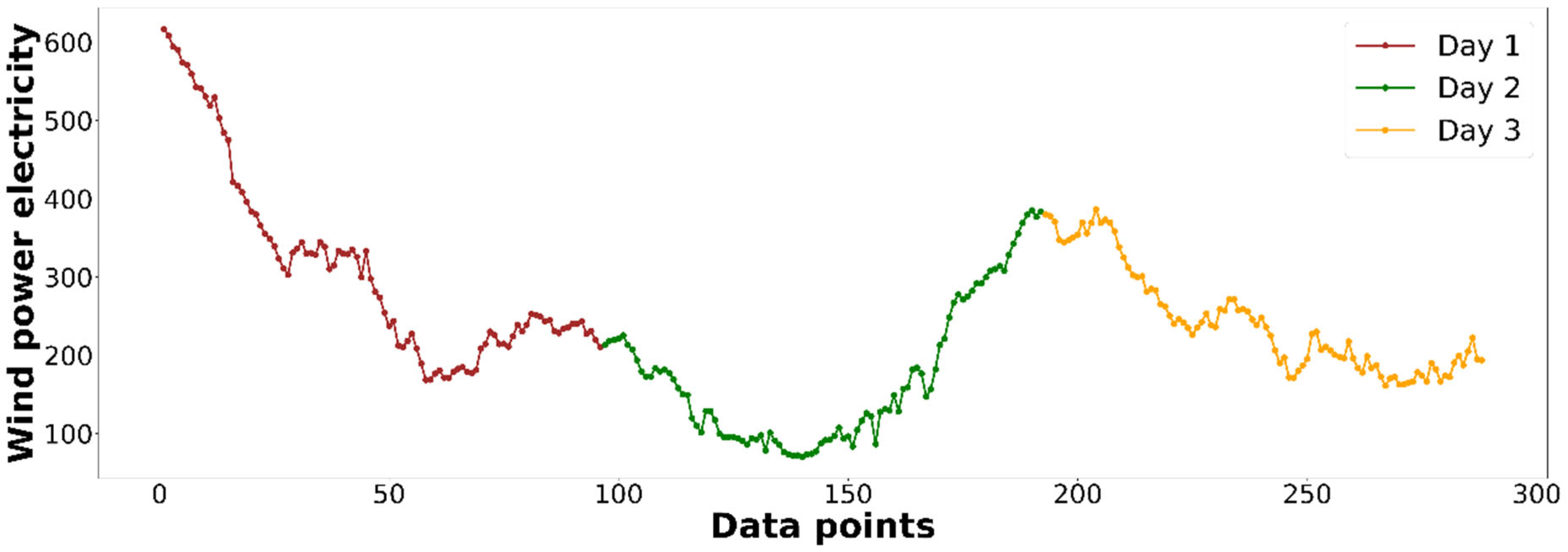
Figure 2 shows an example of the first three days of produced electricity data. As shown in the figure, each day contains a total of 96 recorded $e$ logs because the data are recorded under 15 min cycles from 00:00 to 23:45 per day. Thus, $\mathit{D}$ has a matrix size of $n=3$ $\times$ $TR=96$. Then, based on Equation (1), ${\mathit{d}}_1$ is a vector consisting of 96 $e$ records ($e_{1,1}=616.53,e_{1,2}=608.05,e_{1,3}=594.07,\dots ,e_{1,96}=210.57$), while ${\mathit{d}}_2$ follows the same rule ($e_{2,1}=213.02,e_{2,2}=218.46,e_{2,3}=219.31,\dots ,e_{2,96}=383.3$), and so on. Therefore, the constructed interval-valued data based on the example data are presented in

Table 2. First 3 days of interval-valued data example.

Day	Record 1	Record 2	Record 3	…	Record 96
1	616.53	608.05	594.07	…	210.57
2	213.02	218.46	219.31	…	383.3
3	379.72	377.82	370.56	…	193.64

Note: Ellipses indicate intermediate columns omitted for brevity.

.

2.4.2. Construction of Augmented Features

Once the interval-valued data (matrix $\mathit{D}$) have been prepared, the augmented features are constructed from the data. The augmented features consist of components of the BF and DF. Both are calculated via the intervals of each day, for which they also form the vectors (${\mathit{d}}_{\mathit{i}}$) from matrix $\mathit{D}$.

• BF construction:

The BF includes the upper and lower bounds and central and radius. The upper bound expresses the maximum value in an interval, whereas the lower bound expresses the minimum value. They are denoted by Equations (10) and (11), respectively:

$$\mathrm{U}\mathrm{p}\mathrm{p}\mathrm{e}\mathrm{r}=x_i^U=Max\left({\mathit{d}}_i\right),\mathrm{w}\mathrm{h}\mathrm{e}\mathrm{r}\mathrm{e} i\in {\mathit{Z}}^{+}=1~n$$

(10)

$$\mathrm{L}\mathrm{o}\mathrm{w}\mathrm{e}\mathrm{r}=x_i^L=Min\left({\mathit{d}}_i\right),\mathrm{w}\mathrm{h}\mathrm{e}\mathrm{r}\mathrm{e} i\in {\mathit{Z}}^{+}=1~n.$$

(11)

Following the example data, Upper is the largest value among all 96 records, while Lower is the lowest value among them. Thus, the upper and lower values of the day 1 interval are $Max\left({\mathit{d}}_1\right)=616.53$ and $Min\left({\mathit{d}}_1\right)=168.49$, respectively. The same concept is used to format the upper and lower bounds from the corresponding intervals of each day. After obtaining the upper and lower bounds of each day, they can be further transformed into the central and radius using Equations (12) and (13), respectively:

$$\mathrm{C}\mathrm{e}\mathrm{n}\mathrm{t}\mathrm{r}\mathrm{a}\mathrm{l}=x_i^C={\displaystyle \frac{1}{2}}\left(x_i^U+x_i^L\right),\mathrm{w}\mathrm{h}\mathrm{e}\mathrm{r}\mathrm{e} i\in {\mathit{Z}}^{+}=1~n$$

(12)

$$\mathrm{R}\mathrm{a}\mathrm{d}\mathrm{i}\mathrm{u}\mathrm{s}=x_i^R={\displaystyle \frac{1}{2}}\left(x_i^U-x_i^L\right),\mathrm{w}\mathrm{h}\mathrm{e}\mathrm{r}\mathrm{e} i\in {\mathit{Z}}^{+}=1~n.$$

(13)

Thus, the central and radius values of day 1 from the example are $x_1^C={\displaystyle \frac{1}{2}}\left(x_1^U+x_1^L\right)=392.51$ and $x_1^R={\displaystyle \frac{1}{2}}\left(x_1^U-x_1^L\right)=224.02,$ respectively.

A pair of upper and lower bound values can be extracted from the interval-valued data of each day; thus, $n$ pairs of upper and lower bound values can be extracted from $n$ days of data. This can be expressed as matrix ${\mathit{X}}_{\mathit{i}}^{\mathit{U}\mathit{L}}$, as shown in Equation (14):

$${\mathit{X}}_i^{UL}={\left[\begin{array}{c}{x}_i^U\\ x_i^L\end{array}\right]}^{\mathit{T}}=\left[\begin{array}{c}\begin{array}{c}\begin{array}{cc}{x}_1^U& x_1^L\end{array}\\ ⋮\end{array}\\ \begin{array}{cc}{x}_i^U& x_i^L\end{array}\\ \begin{array}{c}⋮\\ \begin{array}{cc}{x}_n^U& x_n^L\end{array}\end{array}\end{array}\right] \mathrm{w}\mathrm{h}\mathrm{e}\mathrm{r}\mathrm{e} i\in {\mathit{Z}}^{+}.$$

(14)

Following the same concept as that of the upper and lower bounds, each pair of central and radius values can be denoted by ${\mathit{X}}_{\mathit{i}}^{\mathit{C}\mathit{R}}$, as shown in Equation (15):

$${\mathit{X}}_i^{CR}={\left[\begin{array}{c}{x}_i^C\\ x_i^R\end{array}\right]}^{\mathit{T}}=\left[\begin{array}{c}\begin{array}{c}\begin{array}{cc}{x}_1^C& x_1^R\end{array}\\ ⋮\end{array}\\ \begin{array}{cc}{x}_i^C& x_i^R\end{array}\\ \begin{array}{c}⋮\\ \begin{array}{cc}{x}_n^C& x_n^R\end{array}\end{array}\end{array}\right], \mathrm{w}\mathrm{h}\mathrm{e}\mathrm{r}\mathrm{e} i\in {\mathit{Z}}^{+}.$$

(15)

Both ${\mathit{X}}_{\mathit{i}}^{\mathit{U}\mathit{L}}$ and ${\mathit{X}}_{\mathit{i}}^{\mathit{C}\mathit{R}}$ can provide information to describe the boundary of the interval, which can be viewed as an overall profile expression of the interval.

• DF construction:

The structure of an interval can be either symmetric or asymmetric. When the DFs of the mean and median of an interval are equal, with zero skewness, the interval is symmetrically distributed. However, in real-world scenarios, interval-valued data are often asymmetrically distributed and may exhibit complex structures. The DF offers valuable insights into the underlying characteristics of interval-valued data. Hence, utilizing the DF to obtain information that reflects the distribution of an interval can help to enhance the forecasting effectiveness.

The DF consists of the mean, SD, Q1, median, Q3, IQR, skewness, and kurtosis. All of them are constructed using a similar concept to that of the BF in Step 2.1, and calculated via vectors (${\mathit{d}}_{\mathit{i}}$) from matrix $\mathit{D}$. Equations (16)–(23) show the DF calculations.

$$\mathrm{M}\mathrm{e}\mathrm{a}\mathrm{n}=x_i^M=Average\left({\mathit{d}}_i\right)={\displaystyle \frac{1}{TR}}{\sum }_{j=1}^{TR}{e}_{i,j},$$

(16)

where $i\in {\mathit{Z}}^{+}=1~n$.

$$\mathrm{S}\mathrm{D}=x_i^{SD}=Std\left({\mathit{d}}_i\right)=\sqrt{{\displaystyle \frac{1}{TR}}{\sum }_{j=1}^{TR}{(e_{i,j}-x_i^M)}^2},$$

(17)

where $i\in {\mathit{Z}}^{+}=1~n.$

$${\mathrm{Q}}_1=x_i^{Q_1}=Q_1\left({\mathit{d}}_i\right)=\left\{\begin{array}{cc}{e}_{i,j=\left[{\displaystyle \frac{TR}{4}}\right]+1}& ,if{\displaystyle \frac{TR}{4}}\notin {\mathit{Z}}^{+}\\ {\displaystyle \frac{1}{2}}\left(e_{i,j=\left({\displaystyle \frac{TR}{4}}\right)}+e_{i,j=({\displaystyle \frac{TR}{4}}+1)}\right)& ,if{\displaystyle \frac{TR}{4}}\in {\mathit{Z}}^{+}\end{array}\right.,$$

(18)

where $i\in {\mathit{Z}}^{+}=1~n$.

$$\mathrm{M}\mathrm{e}\mathrm{d}\mathrm{i}\mathrm{a}\mathrm{n}=x_i^{MD}=Med\left({\mathit{d}}_i\right)=\left\{\begin{array}{cc}{e}_{i,j=(TR+1)/2}& ,if TR is odd\\ {\displaystyle \frac{1}{2}}\left(e_{i,j=\left({\displaystyle \frac{TR}{2}}\right)}+e_{i,j=({\displaystyle \frac{TR}{2}}+1)}\right)& ,if TR is even\end{array}\right.,$$

(19)

where $i\in {\mathit{Z}}^{+}=1~n.$

$${\mathrm{Q}}_3=x_i^{Q_3}=Q_3\left({\mathit{d}}_i\right)=\left\{\begin{array}{cc}{e}_{i,j=\left[{\displaystyle \frac{3}{4}}TR\right]+1}& ,if {\displaystyle \frac{3}{4}}TR\notin {\mathit{Z}}^{+}\\ {\displaystyle \frac{1}{2}}\left(e_{i,j=\left({\displaystyle \frac{3}{4}}TR\right)}+e_{i,j=({\displaystyle \frac{3}{4}}TR+1)}\right)& ,if {\displaystyle \frac{3}{4}}TR\in {\mathit{Z}}^{+}\end{array}\right.,$$

(20)

where $i\in {\mathit{Z}}^{+}=1~n$.

$$\mathrm{I}\mathrm{Q}\mathrm{R}=x_i^{IQR}=IQR\left({\mathit{d}}_i\right)=x_i^{Q_3}-x_i^{Q_1},$$

(21)

where $i\in {\mathit{Z}}^{+}=1~n$.

$$\mathrm{S}\mathrm{k}\mathrm{e}\mathrm{w}\mathrm{n}\mathrm{e}\mathrm{s}\mathrm{s}=x_i^{SK}=3(x_i^M-x_i^{MD})/x_i^{SD},$$

(22)

where $i\in {\mathit{Z}}^{+}=1~n$.

$$\mathrm{K}\mathrm{u}\mathrm{r}\mathrm{t}\mathrm{o}\mathrm{s}\mathrm{i}\mathrm{s}=x_i^{KU}=Kurtosis\left({\mathit{d}}_i\right)={\displaystyle \frac{\frac{1}{TR}{\sum }_{j=1}^{TR}{\left(e_{i,j}-x_i^M\right)}^4}{({x_i^{SD})}^4}}-3,$$

(23)

where $i\in {\mathit{Z}}^{+}=1~n$.

Following the example data, the DF values of day 1 are $x_1^M=310.29$, $x_1^{SD}=121.99$, $x_1^{Q1}=222.79$, $x_1^{MD}=263.97$, $x_1^{Q3}=345.58$, $x_1^{IQR}=122.78$, $x_1^{SK}=1.04$, and $x_1^{KU}=0.08$.

A set of DFs can be extracted from each day of interval-valued data after construction. Thus, $n$ sets of DFs can be constructed from n days of data, which can be expressed as follows:

$${\mathit{X}}_i^{DF}={\left[\begin{array}{c}{x}_i^M\\ \begin{array}{c}{x}_i^{SD}\\ \begin{array}{c}{x}_i^{Q1}\\ \begin{array}{c}{x}_i^{MD}\\ \begin{array}{c}{x}_i^{Q3}\\ \begin{array}{c}{x}_i^{IQR}\\ \begin{array}{c}{x}_i^{SK}\\ x_i^{KU}\end{array}\end{array}\end{array}\end{array}\end{array}\end{array}\end{array}\right]}^{\mathit{T}}=\left[\begin{array}{c}\begin{array}{ccc}\begin{array}{cc}{x}_1^M& x_1^{SD}\end{array}& \begin{array}{cc}{x}_1^{Q1}& x_1^{MD}\end{array}& \begin{array}{cc}\begin{array}{cc}{x}_1^{Q3}& x_1^{IQR}\end{array}& \begin{array}{cc}{x}_1^{SK}& x_1^{KU}\end{array}\end{array}\end{array}\\ \begin{array}{c}\ddots \\ \begin{array}{c}\begin{array}{ccc}\begin{array}{cc}{x}_i^M& x_i^{SD}\end{array}& \begin{array}{cc}\begin{array}{cc}{x}_i^{Q1}& x_i^{MD}\end{array}& \begin{array}{cc}{x}_i^{Q3}& x_i^{IQR}\end{array}\end{array}& \begin{array}{cc}{x}_i^{SK}& x_i^{KU}\end{array}\end{array}\\ \begin{array}{c}\ddots \\ \begin{array}{ccc}\begin{array}{cc}{x}_n^M& x_n^{SD}\end{array}& \begin{array}{cc}\begin{array}{cc}{x}_n^{Q1}& x_n^{MD}\end{array}& \begin{array}{cc}{x}_n^{Q3}& x_n^{IQR}\end{array}\end{array}& \begin{array}{cc}{x}_n^{SK}& x_n^{KU}\end{array}\end{array}\end{array}\end{array}\end{array}\end{array}\right],$$

(24)

where $i\in {\mathit{Z}}^{+}$.

The augmented features of the BF and DF in each day are constructed from the interval-valued data.

Table 3. Augmented first 3 days of interval-valued data example.

Day	Central	Radius	Upper	Lower	Mean	SD	Q1	Median	Q3	IQR	Skewness	Kurtosis
1	392.51	224.02	616.53	168.49	310.29	121.99	222.79	263.97	345.58	122.78	1.04	0.08
2	227.54	157.44	384.98	70.10	172.71	89.73	95.47	149.53	219.77	124.31	0.86	−0.35
3	273.54	112.52	386.05	161.02	243.67	67.25	189.29	232.25	281.84	92.55	0.73	−0.69

presents all augmented features extracted from the first three days of interval-valued data as an example.

2.4.3. Training of Multi-Step-Ahead Forecasting Model

After completing the construction of the augmented features, they are utilized for the construction of the forecasting model. The proposed AFMIF scheme uses a direct strategy for multi-step-ahead forecasting. The direct strategy is a commonly used multi-step-ahead forecasting strategy with a straightforward concept [46,47]. It forecasts the desired target value at $h$ steps ahead from time period $t$ by directly predicting the outcome while ignoring the information within the future time gap [46,47]. This approach builds forecasting models for different time steps ahead separately, allowing each model to focus on learning specific dynamics when making predictions for each time step. Figure 3 presents a visualized example of constructing models under the direct strategy for multi-step-ahead forecasting. The future time gap refers to the time window between time period $t$ and the desired target step ahead during forecasting; for example, $t+1$ represents forecasting one step ahead. Moreover, as the direct strategy ignores the information within the future time gap, the predictor variables are time-lagged information within the time window of time period $t$. For example, as shown in the figure, information at time period $t$ and time-lagged information at $t-1$ and $t-2$ are used to construct models for multi-step-ahead forecasting.

The forecasting targets in this study are formed from the central and radius and the forecasting is considered as a multi-output forecasting task. As mentioned in the Introduction, as opposed to traditional methods that must forecast both targets separately, DL models can forecast both targets simultaneously, which is more effective than single-output models. Therefore, let $f\left(\right)$ be the forecast model and let the time lag be denoted as $l$. The forecasted central and radius values using the BF and DF as predictors along with the time-lagged information under the direct strategy are expressed as follows:

$${\widehat{x}}_{t+h}^C=f\left({\mathit{X}}_t^{UL},\cdots ,{\mathit{X}}_{t-l+1}^{UL}{,\mathit{X}}_t^{DF},\cdots {,\mathit{X}}_{t-l+1}^{DF}\right), \mathrm{w}\mathrm{h}\mathrm{e}\mathrm{r}\mathrm{e} t\in i={\mathit{Z}}^{+}=\{l,l+1,\cdots ,n-h\}$$

(25)

$${\widehat{x}}_{t+h}^R=f\left({\mathit{X}}_t^{UL},\cdots ,{\mathit{X}}_{t-l+1}^{UL}{,\mathit{X}}_t^{DF},\cdots {,\mathit{X}}_{t-l+1}^{DF}\right),\mathrm{w}\mathrm{h}\mathrm{e}\mathrm{r}\mathrm{e}t\in i={\mathit{Z}}^{+}=\{l,l+1,\cdots ,n-h\},$$

(26)

where the maximum horizon of future steps considered is three steps ahead ($h=(\mathrm{1,2},3)$) and a maximum time-lagged information count of 3 ($l=(\mathrm{1,2},3)$) is considered in this study. Hence, three DL models following the approach of the proposed AFMIF scheme are constructed, namely, AFMIF-GRU, AFMIF-LSTM, and AFMIF-TCN. Furthermore, to confirm the effectiveness of the AFMIF scheme, the simple approach of models using only time-lagged information formed from the targets (central and radius) are constructed for comparison; these models are named S-GRU, S-LSTM, and S-TCN. In addition, SARIMA that is constructed following the simple approach, known as S-SARIMA, is considered for comparison.

All models are built using the expanding window approach based on time when dividing the data into training and testing sets to preserve the chronological order. To ensure fairness and consistency across model comparisons, all three DL models are built using 100 epochs without early stopping, a batch size 64, and the Adam optimizer. ReLU is used as the activation function for all hidden layers, preventing a negative radius, with the linear function for the output layer. Details regarding the DL model structure and corresponding hyperparameters are presented in Supplementary Table S1.

2.4.4. Performance Evaluation

Traditional error metrics evaluate accuracy at the level of single points, measuring the closeness of an estimated point to the corresponding actual point [48]. While these metrics are appropriate for point forecasting, they may be limited or misleading in the interval-valued setting, in which the primary objective is to ensure that the forecasted interval overlaps with the actual interval as closely as possible. Furthermore, the forecasted interval may be wider than the actual interval [48]. Such cases should be considered for appropriate performance evaluation. Thus, the MRXOR metric is used to evaluate the performance of the constructed models when forecasting the GE supply interval. MRXOR considers the overlap of the forecasted and actual intervals [48]. Letting $k$ be the total amount of central and radius data points, the formula for MRXOR is as follows:

$$\mathrm{M}\mathrm{R}\mathrm{X}\mathrm{O}\mathrm{R}={\displaystyle \frac{1}{k}}\sum _{i=1}^k{\displaystyle \frac{‖{\mathit{X}}_i^{CR}∆ {\widehat{\mathit{X}}}_i^{CR}‖}{‖{\mathit{X}}_i^{CR}‖}}=\left\{\begin{array}{c}\begin{array}{cc}{\displaystyle \frac{1}{k}}{\displaystyle \sum _{i=1}^k}{\displaystyle \frac{-2(x_i^R-{\widehat{x}}_i^R)}{2\left(x_i^R\right)}}& if{\widehat{x}}_i^L\le x_i^L\le x_i^U\le {\widehat{x}}_i^U\\ {\displaystyle \frac{1}{k}}{\displaystyle \sum _{i=1}^k}{\displaystyle \frac{2(x_i^R-{\widehat{x}}_i^R)}{2\left(x_i^R\right)}}& if{x}_i^L\le {\widehat{x}}_i^L\le {\widehat{x}}_i^U\le x_i^U\end{array}\\ \begin{array}{cc}{\displaystyle \frac{1}{k}}{\displaystyle \sum _{i=1}^k}{\displaystyle \frac{-2(x_i^C-{\widehat{x}}_i^C)}{2\left(x_i^R\right)}}& if{x}_i^L\le {\widehat{x}}_i^L\le x_i^U\le {\widehat{x}}_i^U\\ {\displaystyle \frac{1}{k}}{\displaystyle \sum _{i=1}^k}{\displaystyle \frac{2(x_i^C-{\widehat{x}}_i^C)}{2\left(x_i^R\right)}}& if{\widehat{x}}_i^L\le x_i^L\le {\widehat{x}}_i^U\le x_i^U\end{array}\end{array}\right.,$$

(27)

where $k=n-l-h+1$; ${\widehat{x}}_i^L={\widehat{x}}_i^C-{\widehat{x}}_i^R$; ${\widehat{x}}_i^U={\widehat{x}}_i^C+{\widehat{x}}_i^R$.

The four conditions reflect how the forecasted interval overlaps with an actual interval that is too wide or too narrow, or inclines to the right or inclines to the left. MRXOR is similar to traditional error metrics in that it ranges from zero upwards, with zero representing the ideal case of perfect estimation. Thus, when comparing the MRXOR of different models, better ones will have smaller values closer to zero.

To evaluate the performance of the AFMIF scheme and reliability of the constructed models, robustness evaluation is performed using an expanding window with different training size proportions (60/70/80/90%) to determine whether the model maintains reasonably stable performance across varying training horizons. This approach repeatedly trains the model for the time-series forecasting task, as random data splitting is not suitable; it would break the temporal dependency and disrupt the chronological order. The experiments in this study were implemented in Python version of 3.8.8 [49] and Jupyter Notebook version 6.3.0 [50]. All forecasting models were constructed using the open-source Python packages Scikit-learn (version 0.24.2) [51,52], Keras (version 2.4.3) [53], TensorFlow (version 2.3.0) [54], PyTorch (version 2.3.0) [55], and statsmodels (version 0.14.0) [56].

3. Empirical Results

3.1. Wind Power Data

The wind-power-based GE supply data used to demonstrate the proposed AFMIF scheme in this study were sourced from the Open Power System Data (OPSD) (https://open-power-system-data.org/, accessed on 1 September 2024). The OPSD is an open-access platform that provides high-quality, structured, and freely available datasets for power system research and analysis [57]. Two different datasets of GE supply data in Belgium and Germany were used. Germany is one of the largest producers of wind energy in Europe, making it a representative case for large-scale integration. In contrast, Belgium operates at a relatively smaller scale but with consistent recent growth [58,59]. The two countries differ in terms of the integration scale and operating environment, allowing for the applicability of the proposed framework to be evaluated across contexts with different wind power backgrounds.

The dataset for Belgium covers data from January 2013 to May 2017, whereas the Germany dataset covers data from January 2013 to September 2020. Moreover, the data of both were recorded under daily cycles of 15 min per electricity log, resulting in a total of 96 electricity logs recorded in each day. Both datasets follow the introduced process for generating interval-valued data with no missing values, resulting in Belgium and Germany having sample sizes of 1600 and 2830, respectively. For clarity, the datasets from Belgium and Germany are named BE15 and GER15, respectively, in this study.

Table 4. Descriptive statistics of augmented features from BE15 and GER15 datasets.

Augmented Features		BE15	GER15
Basic Feature (BF)	Upper	427.94 (267.97)	16,666.27 (11,726.67)
	Lower	111.92 (146.02)	6857.93 (7687.09)
	Central	269.93 (193.30)	11,762.10 (9362.54)
	Radius	158.01 (95.93)	4904.17 (3262.81)
Distribution Feature (DF)	Mean	250.23 (208.49)	11,437.16 (9710.70)
	SD	90.86 (61.83)	3009.66 (2187.26)
	Q1	176.98 (188.05)	8961.48 (8878.69)
	Median	242.17 (221.01)	11,234.96 (10,050.65)
	Q3	317.00 (247.23)	13,837.61 (11,018.07)
	IQR	140.03 (115.19)	4876.13 (4104.66)
	Skewness	0.38 (0.71)	0.20 (0.60)
	Kurtosis	−0.40 (1.32)	−0.80 (0.72)

presents the descriptive statistics of the augmented features generated from the two datasets. As shown in the table, as the wind power background and scale differ in the two countries, with Germany having a larger scale, the statistical values are significantly different.

Figure 4 and Figure 5 present the original profile and generated upper and lower bounds of BE15 and GER15. In both figures, the top panel (a) displays the original raw GE supply data profile and the horizontal axis indicates the year; the bottom panel (b) displays the upper and lower bounds of the interval-valued data. The profile of the original data and interval-valued upper and lower bound data appear similar because the interval data were generated by extracting the daily maximum and minimum values from the 96 records, as explained in the Section 2. This process can be viewed as a reduction in data resolution.

3.2. Model Results

First, the training size of 80% is discussed.

Table 5. MRXOR comparison of models with AFMIF and simple approach using BE15 data.

Approach	Model	One-Step-Ahead	Two-Steps-Ahead	Three-Steps-Ahead	Mean	Overall Mean
Simple	S-SARIMA	1.0215	1.0112	1.0119	1.0149	1.0149
	S-GRU	0.6709	0.8476	0.8801	0.7995	0.9133
	S-LSTM	0.7003	0.8436	0.8884	0.8108
	S-TCN	0.9209	1.0411	1.4269	1.1296
AFMIF	AFMIF-GRU	0.6604	0.8440	0.8673	0.7906	0.8716
	AFMIF-LSTM	0.6916	0.8432	0.8701	0.8016
	AFMIF-TCN	0.7025	1.0370	1.3283	1.0226

presents the forecasting results of models with different approaches for multi-step-ahead forecasting on the BE15 data. As shown in Table 5, in the simple approach, both S-GRU and S-LSTM outperformed S-SARIMA across all time steps, while TCN-S performed better than SARIMA-S in one-step-ahead forecasting. This confirms the reasonable usage of DL methods and the superiority of the GRU and LSTM compared with the classic SARIMA. Next, in terms of the AFMIF approach when forecasting different time steps ahead, AFMIF-GRU performed the best in one-step- and three-steps-ahead forecasting, while exhibiting a close but inferior performance to AFMIF-LSTM in two-steps-ahead forecasting. This difference is likely owing to the dynamic nature of the data and varying patterns of forecasting uncertainty across different time horizons, resulting in different model reactions. The mean in Table 5 is the average of each model’s MRXOR across all time-steps-ahead forecasting. According to the table, AFMIF-GRU was the best model, with a mean MRXOR of 0.7906. In addition, to better demonstrate the overall performance of the proposed AFMIF approach, the overall mean values between S-SARIMA, the simple approach, and the AFMIF approach are compared. As indicated in the table, AFMIF, with an overall mean of 0.8716, performed better than both S-SARIMA and the simple approach. Therefore, AFMIF demonstrated better forecasting effectiveness than the simple approach and the capability for multi-step-ahead forecasting, while AFMI-GRU appeared to be the best-performing model in the BE15 data.

To confirm the performance of AFMIF-GRU further, Figure 6 displays the test results for each AFMIF-based model and S-SARIMA. As shown in the figure, the forecasted central and radius were converted into upper and lower bounds and the intervals within the boundaries were filled with color shading for better visualization to compare them with the actual intervals (marked with blue color). In each set of panels, a1 to a3 present the AFMIF-GRU one-step- to three-steps-ahead forecasts and are marked in red; b1 to b3 present the AFMIF-LSTM one-step- to three-steps-ahead forecasts and are marked in green; c1 to c3 present the AFMIF-TCN one-step- to three-steps-ahead forecasts and are marked in orange; and d1 to d3 present the S-SARIMA one-step- to three-steps-ahead forecasts and are marked in brown. The effectiveness of the forecasting results can be assessed by how well the forecasted interval overlaps with and closely follows the profile of the actual interval. For the one-step-ahead forecasting, it can be observed that, with the proposed AFMIF scheme, the forecasted intervals of all three DL methods (panels a1, b1, and c1) aligned well with the actual interval, with AFMIF-GRU demonstrating the best performance in closely following the profile of the actual interval. Moreover, compared with the S-SARIMA one-step-ahead forecasting (panel d1), the sudden spikes of the interval could be captured more effectively with the proposed AFMIF scheme. For the two- and three-steps-ahead forecasting, the drop in performance was noticeable owing to the longer time step ahead, but AFMIF-GRU remained reasonably well-fitted to the actual interval. With these results presented in Figure 6, the performance of AFMIF-GRU, as indicated in Table 5, is further confirmed, and the effectiveness of the proposed AFMIF scheme is demonstrated.

The effectiveness of AFMIF was also evaluated using the GER15 data with the same settings as those for the BE15 data. Similar circumstances to those found in the BE15 data could be observed in the GER15 data. As shown in

Table 6. MRXOR comparison of models with AFMIF and simple approach using GER15 data.

Approach	Model	One-Step-Ahead	Two-Steps-Ahead	Three-Steps-Ahead	Mean	Overall Mean
Simple	S-SARIMA	1.1041	1.3162	1.4678	1.2960	1.2960
	S-GRU	0.7835	1.0557	1.1332	0.9908	1.1684
	S-LSTM	0.7861	1.2203	1.1979	1.0681
	S-TCN	1.0400	1.7147	1.5846	1.4464
AFMIF	AFMIF-GRU	0.7554	1.0402	1.1201	0.9719	1.0837
	AFMIF-LSTM	0.7737	1.1966	1.1785	1.0496
	AFMIF-TCN	0.9249	1.3383	1.4258	1.2297

, the DL methods with the simple approach performed better than S-SARIMA, which further validated the DL method usage in this study. AFMIF-GRU also showed superior performance as the top model in the GER15 data, with a mean MRXOR of 0.9719. Moreover, a comparison of the overall means shows that AFMIF maintained better performance than S-SARIMA and the simple approach, with a value of 1.0837. Thus, the promising performance of the proposed AFMIF approach was demonstrated with the BE15 and GER15 data, as well as the capability of the AFMIF scheme for multi-step-ahead forecasting.

Comparing the DL methods with the AFMIF approach in both datasets at different time-steps-ahead forecasting according to the information in

Table 7. Model MRXORs with AFMIF approach comparison between BE15 and GER15 data for multi-step-ahead forecasting.

h-Steps-Ahead	Data	AFMIF-GRU	AFMIF-LSTM	AFMIF-TCN
One-step-ahead	BE15	0.6604	0.6916	0.7025
	GER15	0.7554	0.7737	0.9249
	Mean	0.7079	0.7327	0.8137
Two-steps-ahead	BE15	0.8440	0.8432	1.0370
	GER15	1.0402	1.1966	1.3383
	Mean	0.9421	1.0199	1.1877
Three-steps-ahead	BE15	0.8673	0.8701	1.3283
	GER15	1.1201	1.1785	1.4258
	Mean	0.9937	1.0243	1.3771

, the superiority of AFMIF-GRU is clearly demonstrated. By averaging the MRXOR values in each dataset, AFMIF-GRU achieved the best MRXOR value across all steps ahead, with the one-step-ahead forecasting being the lowest (mean MRXOR = 0.7079). The decreasing performance in the larger time steps ahead was noticeable in both datasets, but remained reasonable for all models. However, the performance of models using the GER15 data was slightly inferior to those using BE15, which may be owing to the natural structure of the actual data. Nonetheless, the performance was consistent among all methods, which shows the reliability of the proposed AFMIF scheme. Overall, AFMIF-GRU exhibited the best performance in both datasets for multi-step-ahead interval-valued forecasting and the promising performance of the AFMIF scheme was confirmed.

The promising potential of the AFMIF scheme could further be demonstrated via the improvement rate that was obtained from the performance of both the BE15 and GER15 datasets for each DL model. The improvement rate was calculated by determining the mean difference between the AFMIF and simple approaches, followed by calculating the ratio of improvement achieved by the AFMIF approach over the simple approach. To compare the overall improvement, the results from both datasets were aggregated by calculating their mean. Equation (28) shows the calculation of the improvement rate:

$$\mathrm{Improvement}=\frac{\mathit{Simple}-\mathit{AFMIF}}{\mathit{Simple}}\times 100\%,$$

(28)

where a positive value indicates a reduction in the error. The proposed AFMIF scheme performed better than the simple approach. To illustrate, the mean MRXORs of S-GRU and AFMIF-GRU for the one-step-ahead forecasting using the two datasets were 0.7272 ($\frac{1}{2}(0.6709+0.7838)$) and 0.7079 ($\frac{1}{2}(0.6604+0.7554)$), respectively. The yielded improvement rate was 2.65% ($100\times (0.7272-0.7079/0.7079$), where a 2.65% reduction in error was observed when incorporating the AFMIF approach. The improvement rate of each DL model is presented in Figure 7, where bar colors of blue, orange, and red correspond to one-step-, two-steps-, and three-steps-ahead forecasting, respectively. According to Figure 7, the performance of each DL method was enhanced for the one-step-, two-steps-, and three-steps-ahead forecasting, especially for the TCN. Although the TCN was less effective than the GRU or LSTM (as shown in Table 7), a significant improvement in the TCN could be observed when incorporating the AFMIF scheme.

3.3. Robustness Evaluation

According to the experiments, AFMIF-GRU was the best model in this study. To ensure that the performance of the GRU was stable and the findings of the experiment were reliable, a robustness evaluation was performed on AFMIF-GRU, S-GRU, and S-SARIMA with both the BE15 and GER15 data. For the robustness evaluation, the model was repeatedly constructed using the same process (as mentioned in the third paragraph) with different proportions of training data. The robustness evaluation for the GRU using the BE15 data is presented in

Table 8. Robustness evaluation of S-SARIMA, S-GRU, and AFMIF-GRU using BE15 data.

Model	Train%	One-Step-Ahead	Two-Steps-Ahead	Three-Steps-Ahead	Overall Mean
S-SARIMA	60%	1.1254	1.3212	1.3950	1.1691
	70%	1.1719	1.2513	1.2658
	80%	1.0215	1.0112	1.0119
	90%	1.1020	1.1708	1.1807
	Mean	1.1052	1.1886	1.2134
S-GRU	60%	0.7062	0.9250	0.9423	0.8445
	70%	0.7115	0.9058	0.9482
	80%	0.6709	0.8476	0.8801
	90%	0.7253	0.9100	0.9606
	Mean	0.7035	0.8971	0.9328
AFMIF-GRU	60%	0.6944	0.9230	0.9411	0.8367
	70%	0.6939	0.8872	0.9464
	80%	0.6604	0.8440	0.8673
	90%	0.7212	0.9014	0.9596
	Mean	0.6925	0.8889	0.9286

. The MRXORs of each model for the one-step-, two-steps-, and three-steps-ahead forecasting under various training data proportions are shown. The MRXOR values remained consistent among the models, with no dramatic changes in performance. Comparing the mean in each step ahead, AFMIF-GRU with mean MRXORs of 0.6925, 0.8889, and 0.9286 for one-step-, two-steps-, and three-steps-ahead forecasting consistently outperformed both S-SARIMA and S-GRU. Moreover, the overall mean, calculated as the average of all MRXOR values from each model, demonstrated the superiority of AFMIF-GRU (0.8367).

Using the same concept as that for BE15, the robustness evaluation using the GER15 data is presented in

Table 9. Robustness evaluation of S-SARIMA, S-GRU, and AFMIF-GRU using GER15 data.

Model	Train%	One-Step-Ahead	Two-Steps-Ahead	Three-Steps-Ahead	Overall Mean
S-SARIMA	60%	1.1716	1.3963	1.5993	1.3303
	70%	1.1202	1.3030	1.4434
	80%	1.1041	1.3162	1.4678
	90%	1.2028	1.3542	1.4847
	Mean	1.1497	1.3424	1.4988
S-GRU	60%	0.9210	1.3132	1.4423	1.1004
	70%	0.8710	1.2485	1.3128
	80%	0.7835	1.0557	1.1332
	90%	0.8147	1.1237	1.1854
	Mean	0.8476	1.1853	1.2684
AFMIF-GRU	60%	0.9169	1.2747	1.4267	1.0831
	70%	0.8433	1.2257	1.3031
	80%	0.7554	1.0402	1.1201
	90%	0.8013	1.1122	1.1772
	Mean	0.8292	1.1632	1.2568

. The GRU with both approaches consistently performed better than S-SARIMA in multi-step-ahead forecasting. The performance of AFMIF-GRU varied slightly with different proportions of training data, but it was acceptable as similar circumstances appeared in S-GRU. With mean MRXORs of 0.8292, 1.1632, and 1.2568 in the one-step-, two-steps-, and three-steps-ahead forecasting, AFMIF-GRU consistently showed superior performance over S-GRU. The overall mean of 1.0831 of AFMIF-GRU also confirmed the effectiveness of the AFMIF approach. Hence, according to the robustness evaluation, the findings of this study are consistent and reliable.

The superior performance of the AFMIF-GRU model in accurately forecasting the upper and lower bounds of the GE supply across multiple time steps can provide additional useful information to support GE management. In real-world GE supply operations, such interval forecasts enable grid operators and energy planners to assess not only the expected production but also the potential variability within a future time window. This allows for more informed decision-making regarding load balancing, reserve allocation, and energy dispatch planning. For example, knowing the likely range of the GE output different steps ahead provides critical lead times for preparing backup generation, adjusting storage systems, or scheduling maintenance, thereby improving reliability and reducing the risk of system failure or uneven supply. In addition, accurate multi-step-ahead forecasting can improve green energy management and GE supply reliability, potentially reducing the reliance on fossil-based power plants.

Although the proposed AFMIF scheme has demonstrated promising results, some limitations remain. While the results showed that incorporating augmented features could benefit the model performance, further efforts are required to improve the model forecasting capability on larger horizons. Validation on both the Belgium and Germany datasets supported the consistency of the proposed scheme, but its versatility may be partially constrained when it is applied to other renewable energy sources such as solar or hydro power, as their data structures differ from that of wind power and may require adaptations to the scheme. Overall, the inherent complexity of interval-valued GE data and the challenge of multi-step-ahead forecasting over extended horizons remain significant. Building on the empirical findings of this study, future research will focus on refining the augmented features and improving the model performance for larger forecasting horizons.

4. Conclusions

This study has proposed the AFMIF scheme for the multi-step-ahead forecasting of interval-valued GE supply data by constructing augmented features such as the BF and DF that represent information on the statistical and dynamic properties hidden within the interval-valued data. Using the actual generated wind power GE data of BE15 and GER15, the proposed AFMIF-GRU showed promising results in multi-step-ahead forecasting, outperforming the traditional SARIMA and simple approaches. The promising model provides accurate estimations of GE supply intervals across different future time horizons, which can enhance decision-making and resource allocation in GE management. This also improves the effectiveness in handling unexpected events, as the forecasted GE intervals serve as early warnings, providing managers with better-informed expectations and more time to react and prepare accordingly. In addition, improved GE management can increase the reliability of green energy, encouraging its adoption. This, in turn, may reduce the reliance on fossil-based power plants and contribute to sustainability. In summary, augmented feature usage can enhance the performance of multi-step-ahead interval-valued forecasting and shows promising potential, as demonstrated with the proposed AFMIF scheme.