Distributed Privacy-Preserving Stochastic Optimization for Available Transfer Capacity Assessment in Power Grids Considering Wind Power Uncertainty

Abstract

The uneven expansion of renewable energy generation in different regions highlights the necessity of accurately assessing the available transfer capability (ATC) in power systems. This paper proposes a distributed probabilistic inter-regional ATC assessment framework. First, a spatiotemporally correlated wind power output model is established using wind speed forecast data and correlation matrices, enhancing the accuracy of wind power forecasting. Second, a two-stage probabilistic ATC assessment optimization model is proposed. The first stage minimizes both generation cost and risk-related costs by incorporating conditional value-at-risk (CVaR), while the second stage maximizes the power transaction amount. Thirdly, a privacy-preserving two-level iterative alternating direction method of multipliers (I-ADMM) algorithm is designed to solve this mixed-integer optimization problem, requiring only the exchange of boundary voltage phase angles between regions. Case studies are performed on the 12-bus, the IEEE 39-bus and the IEEE 118-bus systems to validate the proposed framework. Hence, the proposed framework enables more reliable and risk-aware intraday ATC evaluation for inter-regional power transactions. Moreover, the impacts of risk parameters and wind farm output correlations on ATC and generation cost are further investigated.

1. Introduction

As the proportion of renewable energy increases, the expansion of renewable energy generation in different regions is imbalanced [1]. In some regions with abundant wind resources, large-scale wind power development can lead to significant wind curtailment when there is insufficient electricity demand [2]. Due to the uncertain output of renewable energy, other regions may experience both low renewable energy generation and high load demand, requiring more fossil fuels to balance electricity generation and consumption [3]. Therefore, if the inter-regional power supply will be able to balance power flows more flexibly, which will facilitate renewable energy integration and help reduce reliance on fossil fuels. In order to coordinate the inter-regional power transactions, it is necessary to obtain accurate information regarding the transferable power capacity between regions. This requirement highlights the importance of assessing the available transfer capability (ATC) which refers to the remaining transfer capacity from source areas to sink areas, which are available for intraday inter-regional transactions beyond the existing commitments [4].

Currently, extensive research on the assessment of ATC has been conducted. Conventionally, ATC is assessed in deterministic calculation methods. In reference [5], ATC is evaluated through progressive increase in power transaction between the source and the sink areas until the transmission limit is reached. In reference [6], this method is simplified through DC power flow approximation to assess ATC fast in a linear model. Another deterministic method to assess ATC is using two-stage optimization model where the first stage is to minimize the generation cost while the second stage is to maximize the power transaction amount [7,8]. Further limiting the decision variables in the source and the sink areas, reference [4] proposes a transfer-based constrained OPF method for the assessment.

However, these deterministic methods typically calculate ATC without considering the impact of the system uncertainties. Therefore, the probabilistic ATC assessment methods have been further considered. The most common approach is to apply Monte Carlo Simulation which randomly samples the system states and wind power output. For each sample, deterministic methods are then used to calculate ATC [9]. This method allows for the estimation of statistical characteristics such as expectation and variance of ATC [10]. To further consider the spatiotemporal correlations of the wind speed, the correlation matrices are established to align the simulated wind speeds with the measured wind speeds [11]. Another popular probabilistic method is probabilistic optimization. For example, the probabilistic ATC evaluation method in [12] is devised based on probabilistic power flow considering the wind power uncertainty. Reference [13] proposes a robust probabilistic ATC assessment method that considers uncertain wind powers, dynamic line capacities and load fluctuations, ensuring sufficient transmission reliability margin. References [14,15] further discuss the impact of wind power uncertainty on probabilistic ATC evaluation. As demonstrated in reference [16], wind power uncertainty increases the operational risk-related costs. Therefore, reference [17] introduces conditional value-at-risk (CVaR) to quantify this impact of risk cost, which is applied in the ATC assessment.

The aforementioned ATC assessment methods are all centralized calculation approaches, executed by the independent system operator (ISO) with access to the full information of the whole power grids. As the power system scales up, calculating ATC is of great computation burden. Concurrently, Many ISOs refuse to share operational data due to the concerns over their confidentiality, rendering the centralized approach impractical for inter-regional ATC assessment. This necessitates the adoption of distributed methods.

Reference [18] introduces the auxiliary problem principle for real-time ATC assessment in multi-area systems. Reference [19] proposes a network decomposition method, where each area employs REI-type network to represent neighboring areas, facilitating distributed ATC computation across regions. These distributed methods require data exchange between all regions, which raises concerns regarding privacy preservation. If the information shared between regions is limited to boundary information, the privacy of each ISO can be well protected [20]. Reference [21] highlights that the alternating direction multipliers method (ADMM) reduces the amount of data exchanged limiting to only adjacent regions. Similar approaches have also been adopted in other studies: reference [22] employs limited exchange of information to preserve privacy in peer-to-peer energy trading, while reference [23] protects the household consumption data and usage patterns in the energy community. In addition, ADMM algorithm has found broad applications in distributed optimization, including multi-agent learning [24], mobile computing in the Internet of things [25], and federated learning [26], further demonstrating its effectiveness in distributed optimization and privacy protection. Additionally, to handle the binary variables in the model, the iterative ADMM (I-ADMM) has been investigated in the former research. For example, reference [27] proves that I-ADMM converges within finite iterations to a suboptimal solution in the generation unit scheduling problem, while reference [28] applies a similar approach to the optimal transmission switching problem.

To address above issues, this paper proposes a distributed probabilistic inter-regional ATC assessment framework. First, a spatiotemporally correlated wind power output model is established using wind speed forecast data and correlation matrices. Second, a two-stage probabilistic ATC assessment optimization model is proposed: the first-stage optimization model minimizes the generation cost and the risk-related costs, while the second-stage model maximizes the power transaction amount by maximizing the load demand of the sink area and the generator output of the source area. Last, an adaptive-step I-ADMM approach is implemented, limiting data exchanged to only the boundary voltage phase angle, ensuring both privacy preservation and calculation efficiency.

The paper is organized as follows: Section 2 introduces the wind power output model with spatiotemporal correlations, Section 3 presents the probabilistic ATC assessment optimization model, Section 4 details the I-ADMM optimization algorithm and workflow, Section 5 demonstrates simulation results, and Section 6 concludes with research contributions.

2. Wind Power Output Model Incorporating Spatiotemporal Wind Speed Correlations

This section focuses on developing a wind farm output model that captures the spatiotemporal correlations in wind speed prediction errors. First, the forecasted wind speed values for the location of the wind turbine are obtained through sophisticated meteorological simulation tools. Then, the independent and identically distributed Gaussian random matrix W_h is modified to represent the uncorrelated wind speed prediction errors. To account for the spatiotemporal correlation of prediction errors, a set of spatiotemporal covariance matrices are constructed, which modify W_h to create wind speed prediction errors with temporal and spatial correlations. Based on these predictions and the error matrices, wind speed scenarios are generated. These scenarios are then converted into actual wind farm power output scenarios using the wind turbine power curve.

According to the simulation results, the wind speed forecast matrix F can be formed as follows:

$$F=\left[\begin{array}{cccc}{f}_{W,11}& f_{W,12}& \cdots & f_{W,1N_H}\\ f_{W,21}& f_{W,22}& \cdots & f_{W,2N_H}\\ ⋮& ⋮& f_{W,it}& ⋮\\ f_{W,N_{w}1}& f_{W,N_{w}2}& \cdots & f_{W,N_w{N}_H}\end{array}\right]$$

(1)

where f_W,it it is the wind speed forecast at the location of wind turbine i at time step t. N_w is the number of the wind turbines while N_H is the number of the time steps.

In each scenario, a Gaussian random matrix W_h is constructed, whose elements are assumed to be independent and identically distributed (i.i.d), representing the wind speed prediction errors. W_h is presented as follows:

$$W_h=\left[\begin{array}{cccc}{w}_{h,11}& w_{h,12}& \cdots & w_{h,1N_H}\\ w_{h,21}& w_{h,22}& \cdots & w_{h,2N_H}\\ ⋮& ⋮& w_{h,it}& ⋮\\ w_{h,N_{w}1}& w_{h,N_{w}2}& \cdots & w_{h,N_w{N}_H}\end{array}\right]$$

(2)

where w_h,it is the independent and identically distributed Gaussian random variable which stands for the uncorrelated prediction error.

To incorporate spatial correlations among different wind turbines, a spatial correlation matrix R_s,h of size N_w × N_w is constructed:

$$R_{\mathrm{S},h}=\left[\begin{array}{cccc}{\mathrm{\rho }}_{\mathrm{S},11}& {\mathrm{\rho }}_{\mathrm{S},12}& \cdots & {\mathrm{\rho }}_{\mathrm{S},1N_w}\\ {\mathrm{\rho }}_{\mathrm{S},21}& {\mathrm{\rho }}_{\mathrm{S},22}& \cdots & \cdots \\ \cdots & \cdots & {\mathrm{\rho }}_{\mathrm{S},ab}& \cdots \\ {\mathrm{\rho }}_{\mathrm{S},N_{\mathrm{w}}1}& \cdots & \cdots & {\mathrm{\rho }}_{\mathrm{S},N_w{N}_w}\end{array}\right]$$

(3)

where ρ_S,ab is the spatial correlation of wind speed prediction errors at the location of wind turbine (a, b).

Given the symmetric nature of the spatial correlation matrix R_S,h, singular value decomposition (SVD) is applied to obtain its decomposed matrices:

$$R_{\mathrm{S},h}=U_{R_{\mathrm{S},h}}{\sum }_{R_{\mathrm{S},h}}{U}_{R_{\mathrm{S},h}}^{\mathrm{T}}=U_{R_{\mathrm{S},h}}{\sum }_{R_{\mathrm{S},h}}^{1/2}{(U_{R_{\mathrm{S},h}}{\sum }_{R_{\mathrm{S},h}}^{1/2})}^{\mathrm{T}}$$

(4)

where ${\mathbf{U}}_{{\mathrm{R}}_{\mathrm{S},\mathrm{h}}}$ is the unitary matrix obtained after decomposition; ${\Sigma }_{{\mathrm{R}}_{\mathrm{S},\mathrm{h}}}$ is the diagonal matrix with diagonal elements being the singular values arranged in descending order.

The decomposed matrices are used to modify W_h on an hourly basis, resulting in NH individual separate spatially correlated wind speed prediction errors matrices W_S,h, and it can be formulated as follows:

$$W_{\mathrm{S},h}=U_{R_{\mathrm{S},h}}{\Sigma }_{R_{\mathrm{S},h}}^{1/2}{W}_h, h=1,2,\cdots ,N_H$$

(5)

Then, all W_S,h matrices are concatenated to form the matrix W_S representing spatially correlated wind speed prediction errors:

$$W_{\mathrm{S}}=\left[\begin{array}{cccccc}{W}_{\mathrm{S},1}& W_{\mathrm{S},2}& \cdots & W_{\mathrm{S},h}& \cdots & W_{\mathrm{S},N_H}\end{array}\right]$$

(6)

Additionally, the wind speed prediction error matrix W_S must account for the temporal autocorrelation and variance. Construct the temporal autocorrelation vector ρ_T,ω and the variance vector σ_T,ω as follows:

$${\mathbf{\rho }}_{\mathrm{T},\omega }=\left[\begin{array}{cccccc}{\rho }_{\mathrm{T},\omega 1}& {\rho }_{\mathrm{T},\omega 2}& \cdots & {\rho }_{\mathrm{T},\omega h}& \cdots & {\rho }_{\mathrm{T},\omega N_H}\end{array}\right]$$

(7)

$${\mathbf{\sigma }}_{\mathrm{T},\omega }=\left[\begin{array}{cccccc}{\sigma }_{\mathrm{T},\omega 1}& {\sigma }_{\mathrm{T},\omega 2}& \cdots & {\sigma }_{\mathrm{T},\omega h}& \cdots & {\sigma }_{\mathrm{T},\omega N_H}\end{array}\right]$$

(8)

The temporal autocorrelation matrix R_T,ω is constructed as follows:

$$R_{\mathrm{T},\omega }=\left[\begin{array}{cccc}{\rho }_{\mathrm{T},\omega 1}& {\rho }_{\mathrm{T},\omega 2}& \cdots & {\rho }_{\mathrm{T},\omega N_{\mathrm{H}}}\\ {\rho }_{\mathrm{T},\omega 2}& {\rho }_{\mathrm{T},\omega 1}& \cdots & \cdots \\ \cdots & \cdots & \cdots & \cdots \\ {\rho }_{\mathrm{T},\omega N_{\mathrm{H}}}& \cdots & \cdots & {\rho }_{\mathrm{T},\omega 1}\end{array}\right]$$

(9)

where the element in the p-th row and f-th column of R_T,ω is equal to the (|p − f| + 1)-th element of ρ_T,ω.

The variance matrix V_T,ω is a diagonal matrix constructed from the elements of the variance vector σ_T,ω as follows:

$$V_{\mathrm{T},\omega }=\mathrm{diag}\left\{{\mathbf{\sigma }}_{\mathrm{T},\omega }\right\}$$

(10)

By using the temporal autocorrelation matrix R_T,ω and the variance matrix V_T,ω, the temporal covariance matrix K_T,ω is constructed as follows:

$$K_{\mathrm{T},\omega }=V_{\mathrm{T},\omega }{R}_{\mathrm{T},\omega }{V}_{\mathrm{T},\omega }$$

(11)

Similarly, SVD of the temporal covariance matrix K_T,ω is performed to obtain the decomposed matrices as follows:

$$K_{\mathrm{T},\omega }=U_{R_{\mathrm{T},\omega }}{\Sigma }_{R_{\mathrm{T},\omega }}^{1/2}{\left(U_{R_{\mathrm{T},\omega }}{\Sigma }_{R_{\mathrm{T},\omega }}^{1/2}\right)}^{\mathrm{T}}$$

(12)

where ${\mathbf{U}}_{{\mathrm{R}}_{\mathrm{T},\omega }}$ is the unitary matrix obtained after decomposition; ${\Sigma }_{{\mathrm{R}}_{\mathrm{T},\omega }}$ is the diagonal matrix with diagonal elements being the singular values arranged in descending order.

In each scenario, considering spatial correlation, the prediction error matrix with both temporal and spatial correlations, W_ST, is constructed using the unitary and diagonal matrices obtained from the decompositions in Equations (4) and (12), as follows:

$$W_{\mathrm{ST}}=U_{R_{\mathrm{S},h}}{\Sigma }_{R_{\mathrm{S},h}}^{1/2}{W}_h{\left(U_{R_{\mathrm{T},\omega }}{\Sigma }_{R_{\mathrm{T},\omega }}^{1/2}\right)}^{\mathrm{T}}$$

(13)

The wind speed matrix v can be considered as the superposition of the wind speed forecast matrix F and the wind speed prediction error matrix W_ST, described as follows:

$$v=F+W_{\mathrm{ST}}$$

(14)

In each scenario, the random matrix W_h is generated once using Equation (2), from which different wind speed matrices v are independently derived based on Equation (14). This process allows the generation of multiple wind speed scenarios.

The output power of a wind turbine is closely related to the wind speed and its power curve. The model which describes the wind power curve is given by:

$$P_{\mathrm{w}}(v)=\left\{\begin{array}{cc}0,& v>v_0,v<v_{\mathrm{i}}\\ P_{\mathrm{r}}{\displaystyle \frac{v-v_{\mathrm{i}}}{v_{\mathrm{r}}-v_{\mathrm{i}}}},& v_{\mathrm{i}}⩽v⩽v_{\mathrm{r}}\\ P_{\mathrm{r}},& v_{\mathrm{r}}<v<v_0\end{array}\right.$$

(15)

Based on Equation (15), the predicted wind power output forecast P_wi,t is derived from the wind speed forecast matrix F. For each scenario s, the actual wind power output $P_{\mathrm{wi},\mathrm{t}}^{\mathrm{T},\mathrm{s}}$ is obtained from the wind speed matrix v, which incorporates both temporal and spatial uncertainties.

3. Two-Stage Probabilistic ATC Assessment Optimization Model with CVaR Incorporation

To address the operational risk arising from wind power output uncertainty, this paper introduces CVaR to quantify the risk-related costs. A two-stage probabilistic ATC assessment optimization model is proposed: the first-stage optimization model minimizes the generation cost and the risk-related costs, while the second-stage model maximizes the power transaction amount by assuming the maximum load demand in the sink area and the maximum generator output in the source area, based on the decisions from the first stage. In order to fully capture the impact of wind power output uncertainty on unit commitment and overall system operating conditions, a Unit Commitment (UC) model is integrated into the first-stage optimization.

3.1. Mathematical Description of CVaR Theory

The uncertainty of wind power output requires the ISO to adjust the output of conventional generating units, resulting in additional fuel costs and adjustment costs. To address this, these costs are defined as the system operation risk-related costs caused by the uncertainty of wind power output. The expression for this is as follows:

$${\Pi }_G={\displaystyle \sum _{s=1}^S{\mathrm{pr}}^s}\left({\displaystyle \sum _{t=1}^{24}{\displaystyle \sum _{i=1}^{N_{\mathrm{G}}}{c}_i^u\Delta P_{i,t}^{u,s}}}+{\displaystyle \sum _{t=1}^{24}{\displaystyle \sum _{i=1}^{N_{\mathrm{g}}}{c}_i^d\Delta P_{i,t}^{d,s}}}\right)$$

(16)

where Π_G represents the risk cost. ${∆P}_{\mathrm{i},\mathrm{t}}^{\mathrm{u},\mathrm{s}}$ denotes the upward adjustment of the output of the unit i at time step t in the s-th wind power forecast error scenario, while ${∆P}_{\mathrm{i},\mathrm{t}}^{\mathrm{d},\mathrm{s}}$ represents the downward adjustment. The ramping-up cost of the unit i is denoted by $c_{\mathrm{i}}^{\mathrm{u}}$, and the ramping-down cost is represented by $c_{\mathrm{i}}^{\mathrm{d}}$. The probability corresponding to the s-th wind power output forecast error scenario is pr^s. N_G and N_g are the numbers of conventional units with upward and downward adjustments in each scenario, respectively, and S is the total number of scenarios.

To quantify the impact of risk costs on the ATC between regions, the CVaR is introduced to quantify the operational risks generated by wind power prediction errors. For different wind power prediction error scenarios, the overall distribution of generation costs is discrete. Under a given confidence level ε ∈ (0, 1), the probability that the generation cost exceeds the Value-at-Risk (VaR) is (1 − ε) × 100%. The CVaR can be approximated as the expected cost for the scenario set where the probability of higher generation costs is (1 − ε) × 100% [29]. The system operation risk costs due to the uncertainty of wind power output, namely VaR and CVaR, are defined as follows:

$$\mathrm{VaR}=\min \left\{a\in R\mid \phi \left(P_{i,t}^s,a\right)⩾1-\epsilon \right\}$$

(17)

$$\mathrm{CVaR}=a-{\displaystyle \frac{1}{1-\epsilon }}{\displaystyle \sum _{s=1}^s{\mathrm{pr}}^s}\cdot {\eta }^s$$

(18)

where $P_{i,t}^s$ represents the active power output of the conventional generating units under the s-th wind power output forecast error scenario; $\phi (P_{i,t}^s,a)$ denotes the probability that the risk cost Π_G is not less than the threshold a; η^s is the excess value of the total dispatching cost under this scenario, which is a positive number.

3.2. The First-Stage Model of the Two-Stage Optimization Model

In actual power systems operating under normal state, the voltage at each bus generally remains close to the rated value, and the voltage phase angle differences across the lines are relatively small. Furthermore, in high-voltage power networks, the line resistance is much smaller than the line reactance. Thus, the DC power flow model is introduced for simplification.

The first-stage model is a normal-state evaluation model that considers CVaR. It calculates the existing transmission agreements of tie-lines. Its objective function consists of two parts: generation cost and CVaR, and the detailed expression is presented as follows:

$$\min \left[{\displaystyle \sum _{s=1}^S{\mathrm{pr}}^s\left({\displaystyle \sum _{t=1}^{24}{\displaystyle \sum _{i=1}^n(c_i{P}_{i,t}^s+c_i^{su}{n}_{i,t}^{su}+c_i^{sd}{n}_{i,t}^{sd})}}+{\Pi }_{\mathrm{G}}^s\right)}+\beta \cdot \mathrm{CVaR}\right]$$

(19)

where c_i is the generation cost of the unit i ($/MW). $n_{i,t}^{\mathit{su}}$ ($n_{i,t}^{\mathit{sd}}$) is a binary variable which equals 1 if the unit i starts up (shuts down) at time step t. $c_i^{\mathit{su}}$ and $c_i^{\mathit{sd}}$ are, respectively, the cost of start-up and shut-down the unit i. β is the risk factor; ${\Pi }_{\mathrm{G}}^{\mathrm{s}}$ is the risk cost that the system in the scenario s has to bear to maintain power balance due to the uncertainty of wind power output. The CVaR expression is as follows:

$$\begin{array}{c}\mathrm{CVaR}=\min \left(\xi +{\displaystyle \frac{1}{1-\epsilon }}{\displaystyle \sum _{s=1}^S{\mathrm{pr}}^s{\eta }^s}\right)\\ \left({\displaystyle \sum _{t=1}^{24}{\displaystyle \sum _{i=1}^n{c}_i{P}_{i,t}^s}}+c_i^{su}{n}_{i,t}^{su}+c_i^{sd}{n}_{i,t}^{sd}+{\mathrm{pr}}^s\cdot {\Pi }_{\mathrm{G}}^s\right)-\xi ⩽{\eta }^s\\ {\eta }^s⩾0\end{array}$$

(20)

where ξ is an introduced auxiliary variable to represent the VaR, which is determined during the optimization process; η^s is introduced to represent the loss that exceeds VaR.

To meet the real-time power balance requirement, conventional units adjust their output upwards or downwards. The active power balance constraint is formulated as follows:

$${\displaystyle \sum _{i\in {\Omega }_j}\left(P_{i,t}^s+P_{wi,t}\right)}=-{\displaystyle \sum _{l|s_l=j}{P}_{L,l,t}}+{\displaystyle \sum _{l|e_l=j}{P}_{L,l,t}}+P_{\mathrm{Dj},t}+{\displaystyle \sum _{i\in {\Omega }_j}\left(P_{ch,i,t}^{ESS}-P_{dis,i,t}^{ESS}\right)}$$

(21)

$$\begin{array}{l}{\displaystyle \sum _{i\in {\Omega }_j}{P}_{i,t}^s}+{\displaystyle \sum _{i\in {\Omega }_j}{P}_{\mathrm{w}i,t}^{\mathrm{T},s}}-{\displaystyle \sum _{i\in {\Omega }_j\cap N_g}\Delta P_{i,t}^{\mathrm{d},s}}+{\displaystyle \sum _{i\in {\Omega }_j\cap N_G}\Delta P_{i,t}^{\mathrm{u},s}}=\\ -{\displaystyle \sum _{l|s_l=j}{P}_{L,l}^{T,s}}+{\displaystyle \sum _{l|e_l=j}{P}_{L,l}^{T,s}}+P_{\mathrm{Dj},t}+{\displaystyle \sum _{i\in {\Omega }_j}\left(P_{ch,i,t}^{ESS,s}-P_{dis,i,t}^{ESS,s}\right)}\end{array}$$

(22)

where $P_{\mathit{wi},t}^s$ is the active power output of the wind farm and P_Dj,t is the active load at bus j; s_l and e_l are the indices of start and end bus of line l; $P_{L,l}^{T,s}$ denotes the power flow after adjustment of line l in the scenario s. $P_{\mathit{ch},i,t}^{\mathit{ESS}}$ ($P_{\mathit{dis},i,t}^{\mathit{ESS}}$) is the charging (discharging) power of energy storage power plant i.

This paper adopts energy storage plants as energy storage devices for the power system, with limitations on their charging/discharging power, charging/discharging state, and remaining state of charge. The charging and discharging states of the energy storage devices are fixed in each scenario to form the day-ahead plan. The constraints on energy storage are as follows:

$$\left\{\begin{array}{c}0\le P_{ch,j,t}^{ESS}\le u_{ch,j,t}^{ESS}{P}_{ch,j, \max }^{ESS}\hfill \\ \begin{array}{l}0\le P_{dis,j,t}^{ESS}\le u_{dis,j,t}^{ESS}{P}_{dis,j, \max }^{ESS}\\ 0\le P_{ch,j,t}^{ESS,s}\le u_{ch,j,t}^{ESS}{P}_{ch,j, \max }^{ESS}\\ 0\le P_{dis,j,t}^{ESS,s}\le u_{dis,j,t}^{ESS}{P}_{dis,j, \max }^{ESS}\end{array}\hfill \end{array}\right.$$

(23)

$$u_{ch,j,t}^{ESS}+u_{dis,j,t}^{ESS}\le 1$$

(24)

$$\left\{\begin{array}{l}\begin{array}{l}{E}_{j,t}^{ESS}=E_{j,t-1}^{ESS}+P_{ch,j,t}^{ESS}{\eta }_{ch,j}^{ESS}-P_{dis,j,t}^{ESS}/{\eta }_{dis,j}^{ESS}\\ E_{j,t}^{ESS,s}=E_{j,t-1}^{ESS,s}+P_{ch,j,t}^{ESS,s}{\eta }_{ch,j}^{ESS}-P_{dis,j,t}^{ESS,s}/{\eta }_{dis,j}^{ESS}\end{array}\hfill \\ \begin{array}{l}{E}_{j,\min }^{ESS}\le E_{j,t}^{ESS}\le E_{j,\max }^{ESS}\\ E_{j,\min }^{ESS,s}\le E_{j,t}^{ESS,s}\le E_{j,\max }^{ESS,s}\end{array}\hfill \\ \begin{array}{l}\left|E_{j,0}^{ESS}-E_{j,T}^{ESS}\right|\le \Delta E_j^{ESS}\\ \left|E_{j,0}^{ESS,s}-E_{j,T}^{ESS,s}\right|\le \Delta E_j^{ESS}\end{array}\hfill \end{array}\right.$$

(25)

where $u_{\mathit{ch},j,t}^{\mathit{ESS}}$ and $u_{\mathit{dis},j,t}^{\mathit{ESS}}$ represent the charging and discharging states, respectively. $P_{\mathit{ch},j,\mathit{max}}^{\mathit{ESS}}$ and $P_{\mathit{dis},j,\mathit{max}}^{\mathit{ESS}}$ are the charging and discharging power limits of energy storage power plant j. $E_{j,t}^{\mathit{ESS}}$ is the remaining energy capacity of the energy storage power plant. ${\eta }_{\mathit{ch},j}^{\mathit{ESS}}$ and ${\eta }_{\mathit{dis},j}^{\mathit{ESS}}$ are the charging and discharging efficiencies of the energy storage power plant, respectively. $E_{j,\max }^{\mathit{ESS}}$ and $E_{j,\min }^{\mathit{ESS}}$ are the maximum and minimum remaining capacities. ${\Delta E}_j^{\mathit{ESS}}$ is the maximum change in the remaining capacity of energy storage power plant j before and after scheduling.

Before dealing with the power output of the units, the operational status of the unit is evaluated as follows:

$$u_{i,t+1}-u_{i,t}=n_{i,t}^{su}-n_{i,t}^{sd}$$

(26)

where u_i,t is the on/off status of the unit i at time step t, with 1 representing the on status and 0 representing the off status. The on/off status of the units remains fixed in each scenario to form the day-ahead plan.

The unit is subject to ramping limits during operation and must also account for start-up and shut-down events. the constraints are formulated as follows:

$$P_{i,t}^s-P_{i,t-1}^s\le v_i^r{u}_{i,t-1}+P_{i,\min }{n}_{i,t}^{su}$$

(27)

$$P_{i,t-1}^s-P_{i,t}^s\le v_i^r{u}_{i,t}+P_{i,\max }{n}_{i,t}^{sd}$$

(28)

where $v_i^r$ is the ramping speed limit of the unit i.

The scheduling of the units considers both the upper and lower output limits as well as the ramp rate constraints. After adjusting their output, the units’ output must still remain within the specified limits. The unit output constraints are given as follows:

$$u_{i,t}{P}_{i,\min }⩽P_{i,t}^s⩽u_{i,t}{P}_{i,\max }$$

(29)

$$u_{i,t}{P}_{i,\min }⩽P_{i,t}^s-\Delta P_{i,t}^{\mathrm{d},s}⩽u_{i,t}{P}_{i,\max }\hspace{0.33em}\hspace{0.33em}\hspace{0.33em} \forall i\in N_{\mathrm{g}}$$

(30)

$$u_{i,t}{P}_{i.\min }⩽P_{i,t}^s+\Delta P_{i,t}^{\mathrm{u},s}⩽u_{i,t}{P}_{i.\max }\hspace{0.33em}\hspace{0.33em}\hspace{0.33em} \forall i\in N_{\mathrm{G}}$$

(31)

$$0\le \Delta P_{i,t}^{\mathrm{d},s},\Delta P_{i,t}^{\mathrm{u},s}\le 0.5v_i^r$$

(32)

The minimum start-up/shut-down time constraints are formulated as follows:

$$\begin{array}{l}{T}_{on}\left(u_{i,t}-u_{i,t-1}\right)\le {\displaystyle \sum _{\tau =t}^{\min \left\{t+t_{on,\min }-1,T\right\}}{u}_{i,\tau }}\\ T_{on}=\min \left\{t_{on,\min },T-t+1\right\}\end{array}$$

(33)

$$\begin{array}{l}{T}_{off}\left(u_{i,t-1}-u_{i,t}\right)\le {\displaystyle \sum _{\tau =t}^{\min \left\{t+t_{off,\min }-1,T\right\}}\left(1-u_{i,\tau }\right)}\\ T_{off}=\min \left\{t_{off,\min },T-t+1\right\}\end{array}$$

(34)

where t_on,min and t_off,min are, respectively, the minimum duration of start-up/shutdown for the units. To simplify the model, in this paper, all the units are set to the same duration.

Thermal stability constraints are applied to known scenarios. Adjusting the output of conventional units changes the power flow distribution. To ensure line transmission capacity limits are not exceeded, constraints on the changed line power flow are presented as follows:

$$P_{L,l\min }⩽P_{L,l,t}⩽P_{L,l\max }$$

(35)

$$P_{L,l\min }⩽P_{L,l,t}^{t,s}⩽P_{L,l\max }$$

(36)

The power flow of the lines is determined before and after the output adjustment. Based on the transmission line power flow and the reference bus phase constraint, the voltage phase angle constraints before and after the output adjustment are formulated as follows:

$${\theta }_{\mathrm{ref},t }=0$$

(37)

$${\theta }_{\mathrm{ref},t}^{T,s}=0$$

(38)

$$P_{L,l,t}=({\theta }_{s_l,t}-{\theta }_{e_l,t})/x_l$$

(39)

$$P_{L,l,t}^{T,s}=({\theta }_{s_l,t}^{T,s}-{\theta }_{e_l,t}^{T,s})/x_l$$

(40)

where θ_j,t is the voltage phase angle of bus j. ${\theta }_{e_l,t}^{T,s}$. is the voltage phase angle after adjustment in scenario s. x_l is the reactance of line l.

To ensure the stability of the existing regional transmission commitment, the voltage phase angles at both ends of the transmission lines and the power flow through the lines remain fixed before and after the output adjustment:

$${\theta }_{s_l,\psi (s_l)}={\theta }_{s_l,\psi (e_l)},{\theta }_{e_l,\psi (s_l)}={\theta }_{e_l,\psi (e_l)} \forall l\in \mathrm{tie}\text{-}\mathrm{line}$$

(41)

$${\theta }_{s_l,\psi (s_l)}={\theta }_{s_l,\psi (s_l)}^{T,s},{\theta }_{e_l,\psi (s_l)}={\theta }_{e_l,\psi (s_l)}^{T,s} \forall l\in \mathrm{tie}\text{-}\mathrm{line}$$

(42)

$${\theta }_{s_l,\psi (e_l)}={\theta }_{s_l,\psi (e_l)}^{T,s},{\theta }_{e_l,\psi (e_l)}={\theta }_{e_l,\psi (e_l)}^{T,s} \forall l\in \mathrm{tie}\text{-}\mathrm{line}$$

(43)

where ψ (e_l) is the set of tie-lines connected to bus e_l. Constraint (41) is the coupled constraint, limiting the voltage phase angles of buses at the tie-lines.

3.3. The Second-Stage Model of the Two-Stage Optimization Model

The second-stage model of this paper uses the DC power flow model in the maximum transfer state, with its system binary variables set according to the values obtained from the first-stage model. The model aims to maximize the expected inter-regional probabilistic ATC by assuming the maximum load demand in the sink area and the maximum generator output in the source area. Its objective function is given as follows:

$$\max \left[{\displaystyle \sum _{s=1}^s{\mathrm{pr}}^s}\left({\displaystyle \sum _t({\displaystyle \sum _{j\in S\mathrm{ink}}{P}_{Dj,t}^{1,s}}+{\displaystyle \sum _{i\in \mathrm{Source}}{P}_{i,t}^{1,s}})}\right)\right]$$

(44)

where the superscript 1 indicates the maximum transfer state.

In the maximum transfer state, the bus power balance of the system is formulated as follows:

$${\displaystyle \sum _{i\in {\Omega }_j}\left(P_{i,t}^{1,s}+P_{wi,t}^{T,s}\right)}=-{\displaystyle \sum _{l|s_l=j}{P}_{L,l,t}^{1,s}}+{\displaystyle \sum _{l|e_l=j}{P}_{L,l,t}^{1,s}}+P_{Dj,t}^1+{\displaystyle \sum _{i\in {\Omega }_j}\left(P_{ch,i,t}^{1,ESS,s}-P_{dis,i,t}^{1,ESS,s}\right)}$$

(45)

The energy storage constraints of the system in this state are formulated as follows:

$$\left\{\begin{array}{l}0\le P_{ch,j,t}^{1,ESS,s}\le u_{ch,j,t}^{*,ESS}{P}_{ch,j, \max }^{ESS}\\ 0\le P_{dis,j,t}^{1,ESS,s}\le u_{dis,j,t}^{*,ESS}{P}_{dis,j, \max }^{ESS}\end{array}\right.$$

(46)

$$\left\{\begin{array}{l}{E}_{j,t}^{1,ESS,s}=E_{j,t-1}^{1,ESS,s}+P_{ch,j,t}^{1,ESS,s}{\eta }_{ch,j}^{ESS}-P_{dis,j,t}^{1,ESS,s}/{\eta }_{dis,j}^{ESS}\\ E_{j,\min }^{ESS,s}\le E_{j,t}^{1,ESS,s}\le E_{j,\max }^{ESS,s}\\ \left|E_{j,0}^{1,ESS,s}-E_{j,T}^{1,ESS,s}\right|\le \Delta E_j^{ESS}\end{array}\right.$$

(47)

where $u_{\mathit{ch},j,t}^{*,\mathit{ESS}}$ and $u_{\mathit{dis},j,t}^{*,\mathit{ESS}}$ are the charging/discharging state of energy storage power plant j at time step t in the base state, which are determined in the first-stage model and treated as fixed values in this stage.

The unit constraints of the system in this stage are formulated as follows:

$$P_{i,t}^{1,s}-P_{i,t-1}^{1,s}\le v_i^r{u}_{i,t-1}^{*}+P_{i,\min }{n}_{i,t}^{*,su}$$

(48)

$$P_{i,t-1}^{1,s}-P_{i,t}^{1,s}\le v_i^r{u}_{i,t}^{*}+P_{i,\max }{n}_{i,t}^{*,sd}$$

(49)

$$u_{i,t}^{*}{P}_{i,\min }⩽P_{i,t}^{1,s}⩽u_{i,t}^{*}{P}_{i,\max }$$

(50)

where $u_{i,t}^{*}$, $n_{i,t}^{*,\mathit{su}}$ and $n_{i,t}^{*,\mathit{sd}}$ are the statuses of the unit i at time step t in the base state, which are determined in the first-stage model and treated as fixed values in this stage.

When assessing the maximum transfer capacity, the load level of the sink area is maximized while the load level of the source area remains unchanged. The load constraints are given as follows:

$$P_{Dj,t}^1=P_{Dj,t}\hspace{0.33em}\hspace{0.33em}\hspace{0.33em} \forall i\in \mathrm{Source}$$

(51)

$$P_{Dj,t}^1\ge P_{Dj,t}\hspace{0.33em}\hspace{0.33em}\hspace{0.33em} \forall i\in \mathrm{Sin}k$$

(52)

the phase angle and the line transmission constraints of the system are formulated as follows:

$$P_{L,l\min }⩽P_{L,l,t}^{1,s}⩽P_{L,l\max }$$

(53)

$${\theta }_{\mathrm{ref}}^{1,s}=0$$

(54)

$$P_{L,l,t}^{1,s}=({\theta }_{s_l,t}^{1,s}-{\theta }_{e_l,t}^{1,s})/x_l$$

(55)

the constraints on the phase angles at both ends of the transmission lines in the maximum transfer state are given as follows:

$${\theta }_{s_l,\psi (s_l)}^1={\theta }_{s_l,\psi (e_l)}^1,{\theta }_{e_l,\psi (s_l)}^1={\theta }_{e_l,\psi (e_l)}^1 \forall l\in \mathrm{tie}\text{-}\mathrm{line}$$

(56)

4. Solution Methodology

To preserve the independence of each region, the overall model is decoupled into independent models for each subsystem.

Since the first stage introduces binary variables, directly applying the ADMM algorithm would result in non-convergence. Therefore, a two-level I-ADMM algorithm is adopted to solve the problem. The upper level determines the state of the binary variables, while the lower level uses the ADMM algorithm to handle the continuous variables with the binary variables fixed, calculating the existing transmission agreements of tie-lines at base state. The second-stage model is solved by ADMM algorithm, taking the binary variables obtained from the first stage as fixed input.

4.1. Distributed Problem Based on ADMM

Whether in the first stage or the second stage model, the subsystems are coupled with each other based on the voltage phase angles of the buses on the connection lines. By replicating the boundary bus voltage angle information, data exchange between regions is achieved, ensuring consistency across the entire system. This subsection takes the first-stage optimization model as an example.

The coupling constraint in the example model is (41). When partitioning the system, the boundary issue is handled by replicating the information of boundary buses. Taking boundary bus i in source area as an example, the voltage phase angle of bus i in its own region is represented as θ_i,So, and when copied to sink area, it is represented as θ_i,Si. To ensure that the system remains unchanged before and after partitioning, global variables z_i are used to connect the same variable copied into different sub-areas, which can be computed as:

$$z_i=({\theta }_{i,So}+{\theta }_{i,Si})/2$$

(57)

The objective function of the first-stage optimization which consists of multiple independent functions is given as follows:

$$\begin{array}{l}\min {\displaystyle \sum _{s=1}^S{\mathrm{pr}}^s\left({\displaystyle \sum _{t=1}^{24}{\displaystyle \sum _{i=1}^n(c_i{P}_{i,t}^s+c_i^{su}{n}_{i,t}^{su}+c_i^{sd}{n}_{i,t}^{sd})}}+{\Pi }_G^s\right)}\\ +\beta \cdot \mathrm{CVaR}+{\displaystyle \sum _t{\displaystyle \sum _{i\in B{B}_a}[{\lambda }_{i,t}({\theta }_{i,t}-z_{i,t})+0.5\rho {({\theta }_{i,t}-z_{i,t})}^2]}}\end{array}$$

(58)

where BB_a is the set of boundary buses in area a.

With the coupling constraint is relaxed, the subsystems are independent. The first-stage model of each subsystem is with objective (58) and constraints (20)–(40).

4.2. The Solution for the First-Stage Model Based on I-ADMM Algorithm

The procedure of the solution for the first-stage ATC calculation model is carried out using a two-level distributed I-ADMM algorithm. The I-ADMM algorithm consists of an upper level for binary variable coordination and a lower level for handling the continuous variables.

(1) 

Upper level

The upper level solves the overall mixed-integer optimization problem by iteratively alternating between binary variable updates and continuous variable coordination via the lower-level algorithm. The procedure of the upper level is as follows:

Step 1: In this step, set the outer iteration index r = 0, and relax all the binary variables—u_i,t, $n_{i,t}^{\mathit{su}}$, $n_{i,t}^{\mathit{sd}}$, $u_{\mathit{ch},j,t}^{\mathit{ESS}}$ and $u_{\mathit{dis},j,t}^{\mathit{ESS}}$—into continuous variables. Solve the relaxed model with objective (58) and constraints (20)–(40) using the lower-level ADMM algorithm to obtain the global variables $z_{i,t}^r$ at r = 0.

Step 2: Fix $z_{i,t}^r$, restore the binary constraints and solve the original mixed-integer model independently in each subsystem to yield the binary decisions—$u_{i,t}^r$, $n_{i,t}^{\mathit{su},r}$, $n_{i,t}^{\mathit{sd},r}$, $u_{\mathit{ch},j,t}^{\mathit{ESS},r}$ and $u_{\mathit{dis},j,t}^{\mathit{ESS},r}$—for the r-th iteration.

Step 3: Fix the binary variables, and use the lower-level ADMM algorithm to re-solve the continuous problem and update the global variable $z_{i,t}^r$ in the r-th iteration.

Step 4: If the binary variable gap b^r (calculated by (59)) is equal to 0, the algorithm converges and terminates. Otherwise, set r = r + 1 and repeat steps 2–4.

$$\begin{array}{c}{b}^r={‖u_{i,t}^r-u_{i,t}^{r-1}‖}_2^2+{‖n_{i,t}^{su,r}-n_{i,t}^{su,r-1}‖}_2^2+{‖n_{i,t}^{sd,r}-n_{i,t}^{sd,r-1}‖}_2^2\\ +{‖u_{ch,j,t}^{ESS,r}-u_{ch,j,t}^{ESS,r-1}‖}_2^2+{‖u_{dis,j,t}^{ESS,r}-u_{dis,j,t}^{ESS,r-1}‖}_2^2\end{array}$$

(59)

(2) 

Lower level

The lower level adopts the ADMM algorithm to coordinate boundary-coupled continuous variables across regions. To improve convergence behavior and numerical stability, an adaptive penalty update strategy is introduced [30]. The procedure of the lower level is as follows:

Step 1: Initialize the global variable z_i,t = 0 and the Lagrange multipliers λ_i,t = 0. Set the iteration index k = 0.

Step 2: Each ISO independently solves its optimization problem. Afterward, neighboring ISOs exchange the boundary voltage phase angles. At this step, the primal gap r^k and the dual gap s^k are calculated by (60) and (61), respectively. If both r^k and s^k are sufficiently small such that they satisfy (62), the algorithm terminates. Otherwise, the algorithm proceeds to the next iteration with k = k + 1. The related formulations are presented as follows:

$$r^k={‖{\lambda }_{i,t}^k-{\lambda }_{i,t}^{k-1}‖}_2^2$$

(60)

$$s^k={\mathrm{\rho }}^k{‖z_{i,t}^k-z_{i,t}^{k-1}‖}_2^2$$

(61)

$$r^k⩽{\epsilon }_1,s^k⩽{\epsilon }_2$$

(62)

Step 3: The penalty parameter ρ is a critical factor influencing both the convergence rate and stability of the ADMM algorithm. In this step, the penalty parameter is dynamically adjusted based on the current primal gap r^k and dual gap s^k, as described in formulas (63), to accelerate convergence and improve stability. The global variables and the Lagrange multipliers are then updated according to (57) and (64), respectively.

$${\rho }^{k+1}=\left\{\begin{array}{l}{\rho }^k(1+\lg (r^k/s^k\left)\right) r^k\ge 10s^k\\ {\rho }^k{/(1+\lg (s}^k/r^k\left)\right) s^k\ge 10r^k\\ {\rho }^k \mathrm{else}\end{array}\right.$$

(63)

$${\lambda }_{i,t}^{k+1}={\lambda }_{i,t}^k+{\rho }^k\left({\theta }_{i,t}-z_{i,t}^k\right)$$

(64)

Step 4: Repeat steps 2–3 until convergence condition (62) is met. At this point, the resulting solution corresponds to a continuous relaxation of the ATC problem under fixed binary variables.

From Equation (63), when r^k is large, ρ^k+1 increases, causing ${\lambda }_{i,t}^{k+1}$ to grow. This enhancement helps to promote inter-regional convergence and accelerates the convergence of r^k. Conversely, when s^k is large, ρ^k+1 decreases, which limits the rapid growth of ${\lambda }_{i,t}^{k+1}$ helping to avoid oscillations and enhancing stability.

As a result of this two-level procedure, the I-ADMM algorithm provides the existing transmission agreements of tie-lines at the base state. It also determines the binary variables, including unit commitment and operational decisions, such as start-up, shut-down, and energy storage management. These are essential for accurately assessing the maximum transfer capacity between regions.

4.3. The Solution for the Second-Stage Model Based on the ADMM Algorithm

The second-stage ATC calculation model is solved with the following objective function:

$$\begin{array}{l}\min -{\displaystyle \sum _{s=1}^s{\mathrm{pr}}^s}\left({\displaystyle \sum _t({\displaystyle \sum _{j\in S\mathrm{ink}}{P}_{Dj,t}^{1,s}}+{\displaystyle \sum _{i\in \mathrm{Source}}{P}_{i,t}^{1,s}})}\right)\\ +{\displaystyle \sum _t{\displaystyle \sum _{i\in B{B}_a}[{\lambda }_{i,t}({\theta }_{i,t}^1-z_{i,t}^1)+0.5\rho {({\theta }_{i,t}^1-z_{i,t}^1)}^2]}}\end{array}$$

(65)

The second-stage model of each subsystem is with objective (65) and constraints (45)–(55), where the binary variables obtained from the first-stage model are fixed as input. The solution method follows the ADMM algorithm from the first stage, so no further elaboration is needed here.

The second stage calculates the expected inter-regional probabilistic ATC, thereby obtaining the results required for this study.

4.4. Probabilistic ATC Assessment Procedure

In summary, the probabilistic ATC assessment procedure considering wind power output correlation and CVaR proposed in this paper is illustrated in Figure 1. The detailed steps are as follows:

Step 1: The forecasted wind speed values for the location of the wind turbines are obtained through sophisticated meteorological simulation tools. The uncorrelated wind speed prediction errors are represented using an independent and identically distributed Gaussian random variable matrix. A set of spatiotemporal covariance matrices is constructed to account for the spatiotemporal correlation of prediction errors. These matrices are overlaid onto the wind speed prediction values to obtain a series of wind speed scenarios. Finally, derive the wind power output prediction values, considering wind speed correlation across multiple scenarios.

Step 2: Develop a two-stage probabilistic ATC evaluation model incorporating CVaR. The first stage adopts a UC model incorporating CVaR to minimize the generation cost and risk expense, thereby determining the optimal output benchmark value of the unit and the associated binary variables. The second-stage model evaluates the interregional probabilistic ATC under the maximum transfer state with the binary variables fixed.

Step 3: To solve the proposed ATC evaluation model, the ADMM algorithm for distributed problem-solving, ensuring efficient coordination across regions. To handle binary variables in the first stage, a two-level I-ADMM algorithm is adopted. This algorithm consists of an upper level for binary variable coordination and a lower level for handling the continuous variables. To preserve privacy, the data exchanged is limited to only adjacent regions, minimizing exposure of sensitive information. Additionally, an adaptive scheme is introduced to improve the convergence rate and enhance the overall stability of the algorithm.

5. Case Study

This section elaborates the proposed ATC assessment framework. It begins by generating wind speed forecasting scenarios based on the methodology in Section 2. Then the simulations performed based on the 12-bus, the IEEE 39-bus and the IEEE 118-bus systems validate the effectiveness of proposed framework. The impacts of the risk parameters and the wind farm correlation on ATC assessment are investigated by comparing the expected inter-regional probabilistic ATC and total system generation cost.

5.1. Wind Speed Forecasting Scenario Generation

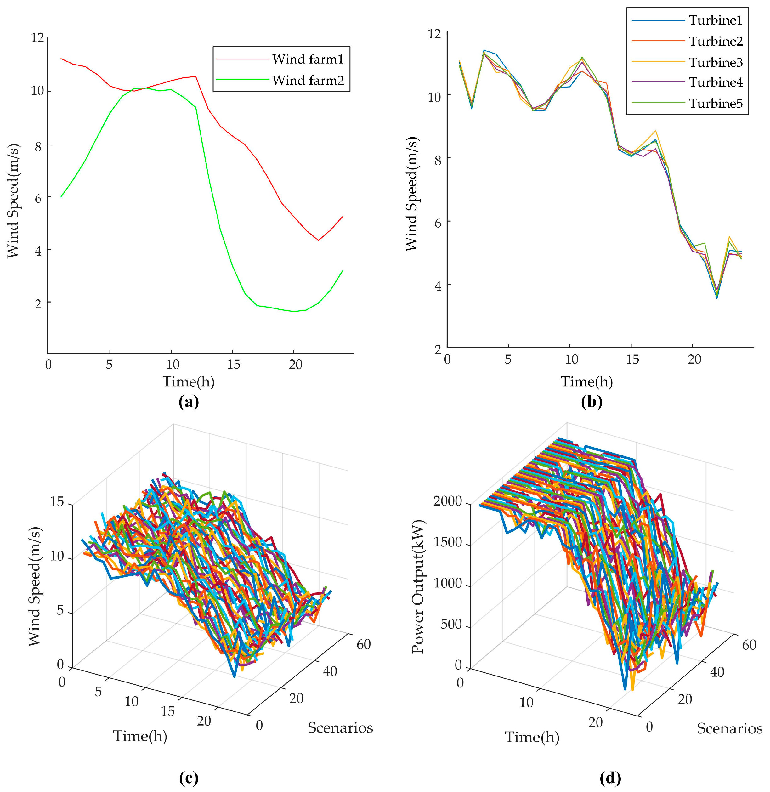
The predicted wind speed values are generated according to the wind speed correlation between wind farms W1 and W2, as described in Section 2. Assuming that each wind farm has five wind turbines, the wind speed correlation ρ_S between turbines in different wind farms is 0.5, while within the same wind farm, it is 0.95. The wind speed prediction matrix F is obtained through the sophisticated meteorological simulation tools. F and the wind speed prediction error matrix W_ST can be used to derive the wind speed prediction matrix with spatiotemporal correlation. Based on this matrix and Equation (15), the wind power output of each wind farm can be calculated. Figure 2 shows the wind speed prediction values with spatiotemporal correlation, where Figure 2a compares the predicted wind speeds between different wind farms, and Figure 2b compares the predicted wind speeds of different turbines within the same wind farm. Figure 2c depicts the wind speed predictions of wind turbine 1 under different scenarios, while Figure 2d depicts the corresponding power output curve based on these wind speed predictions.

5.2. 12-Bus System

All simulations were performed on a personal computer using the Matlab 2022b platform with Gurobi 9.5.1, powered by an Intel Core^TM i7-9750H CPU (2.6 GHz) and 16 GB of memory.

As shown in Figure 3, the 12-bus system’s topology is presented, formed by connecting two 6-bus systems via a tie-line. Each of the two subsystems incorporates 4 generators, 7 transmission lines, 1 wind farm, 1 energy storage power plant, 3 load centers and 6 buses. The wind farm in the sink area includes 5 wind turbines with an installed capacity of 2 MW each, while that in the source area includes 10 wind turbines. Each energy storage station is designed with a power capacity of 200 MW and an energy capacity of 1600 MWh. The remaining parameters of this case study are referenced from the reference [28].

In this experiment, the risk factor β is temporarily set to 2 and the confidence level ε to 0.9 for calculating the system’s probabilistic ATC.

Figure 4 presents the ATC variation over time in the case study. The red bars show the existing transmission commitments power, while the blue bars indicate the ATC. The sum of both bars represents the system’s maximum transferable power. These powers fluctuate due to changes in wind power and the load curve. From 9:00 to 19:00, although the load fluctuates during peak hours, the ATC remains stable during this period and retains a sufficient margin, due to the ample committed generation capacity and adequate tie-line capacity. This time-phased ATC assessment will be shared with both regions. When additional inter-regional transactions occur intraday, these data will serve as the basis for assessing remaining transmission capacity.

During actual operations, ISOs can reflect the level of risk aversion against wind power uncertainty through the confidence level and risk factor. Therefore, this section further investigates the impact of confidence levels and risk factors on ATC calculation results. The proposed model assesses ATC each time step. To analyze the impact of these parameters and make comparisons, the sum of the expected inter-regional probabilistic ATC and the total system operation cost are calculated.

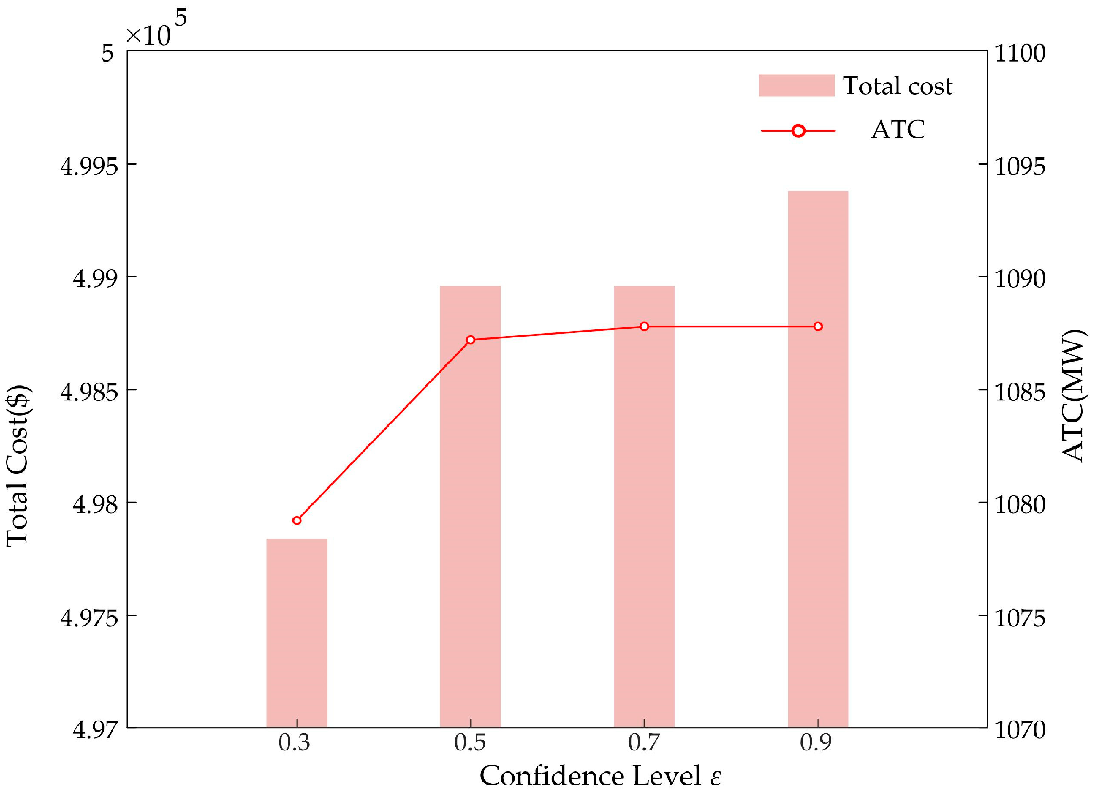
First, the impact of the confidence level on the expected inter-regional probabilistic ATC is analyzed with the risk factor β fixed at 2. Figure 5 demonstrates the impact of different confidence levels on the total system generation cost and the expected inter-regional probabilistic ATC values.

In Figure 5, as the confidence level ε of the total generation cost increases from 0.3 to 0.9, the expected inter-regional probabilistic ATC increases by approximately 15 MW, and the total generation cost continues to rise. As the inter-regional ATC increases, the remaining transmission capacity of the inter-regional tie lines gradually expands to accommodate the most severe fault conditions. Meanwhile, the continuous rise in the total generation cost reflects the ISO’s efforts to mitigate operational risks associated with wind power uncertainty. As a result, the system’s operational reliability is enhanced.

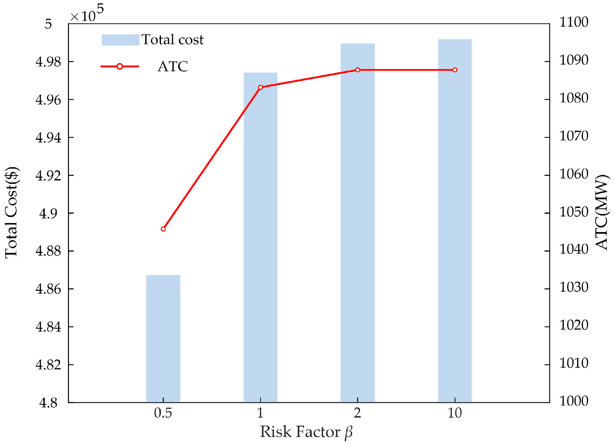
Second, the impact of the risk factor on the expected inter-regional probabilistic ATC is analyzed with the confidence level ε fixed at 0.9. Figure 6 presents the expected inter-regional probabilistic ATC values for risk factors ranging from 0.5 to 10.

According to Equation (19), it can be seen that when the value of risk factor β is relatively small, ISOs that prioritize minimizing generation costs will face an increased risk of cost fluctuations. As the risk factor gradually increases, the ISOs begin to place greater emphasis on avoiding cost fluctuation risk.

When the risk factor is relatively small, as the risk factor increases, the sum of the expected inter-regional probabilistic ATC increases from 1045 MW to 1080 MW, and the total generation cost increases from $4.87 × 10⁵ to $4.97 × 10⁵. When the risk factor is higher, the expected inter-regional probabilistic ATC and total generation cost increase at a slower rate. Compared to the increase in confidence level, the risk factor has a more significant impact on both the expected inter-regional probabilistic ATC and the total generation cost.

The case study above demonstrates that the risk parameters including risk factor and confidence level affect the assessment results of ATC. Therefore, the ISO should set these parameters according to its level of risk aversion in order to accurately evaluate the available transfer capability.

5.3. 39-Bus System

This section extends the case analysis to the IEEE 39-bus system. The partitioned system structure is illustrated in Figure 7. Two wind farms and two energy storage stations are integrated into this system. To further validate the results, this case considers the different spatial correlations of wind power output prediction errors. The wind farm in the sink area includes 15 wind turbines with an installed capacity of 2 MW each, while that in the source area includes 30 wind turbines. Each energy storage station is designed with a power capacity of 200 MW and an energy capacity of 1600 MWh. The remaining parameters of this case study are referenced from the reference [31].

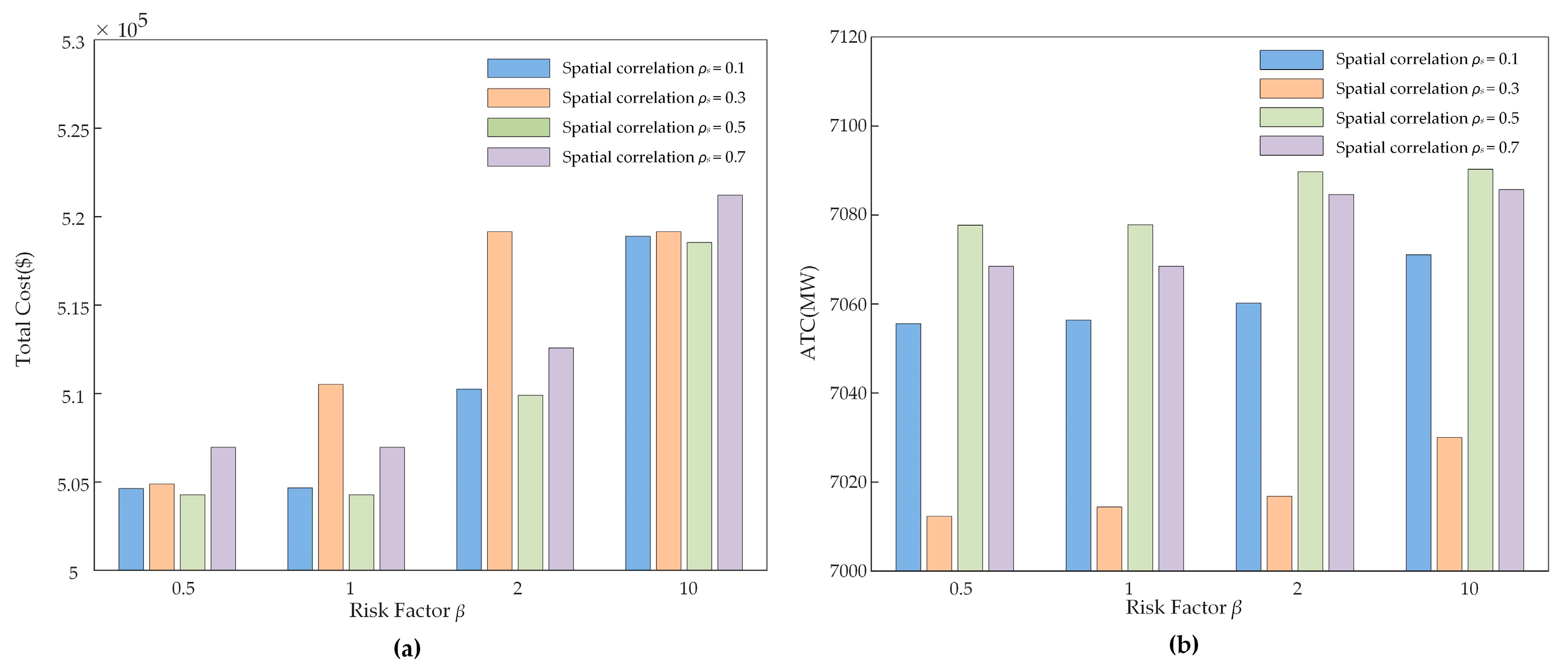
This section analyzes the impact of wind farm output correlation on probabilistic ATC expectation, considering different spatial correlations of wind power output forecast errors. The wind speed correlation ρ_s between turbines in different wind farms is increased from 0.1 to 0.7, while the correlation within each wind farm is fixed at 0.95 and the confidence level is set to 0.9. Figure 8 illustrates total generation cost (a) and the expected probabilistic ATC (b) of the IEEE 39-bus system under varying inter-farm wind speed correlations.

Figure 8 shows the impact of the correlation coefficient on the expected probabilistic ATC value and total generation cost under different risk factors. When the risk factor is 0.5, the expected total generation cost increases as the correlation coefficient rises from 0.1 to 0.7, reflecting stronger inter-farm output correlation. In contrast, when the risk factor is 2, the total generation cost expectation peaks at a correlation coefficient of 0.3. This behavior results from the varying generator dispatch levels driven by different wind power forecast error patterns. Similarly, the inter-regional probabilistic ATC first declines and then increases as the correlation coefficient grows.

5.4. 118-Bus System

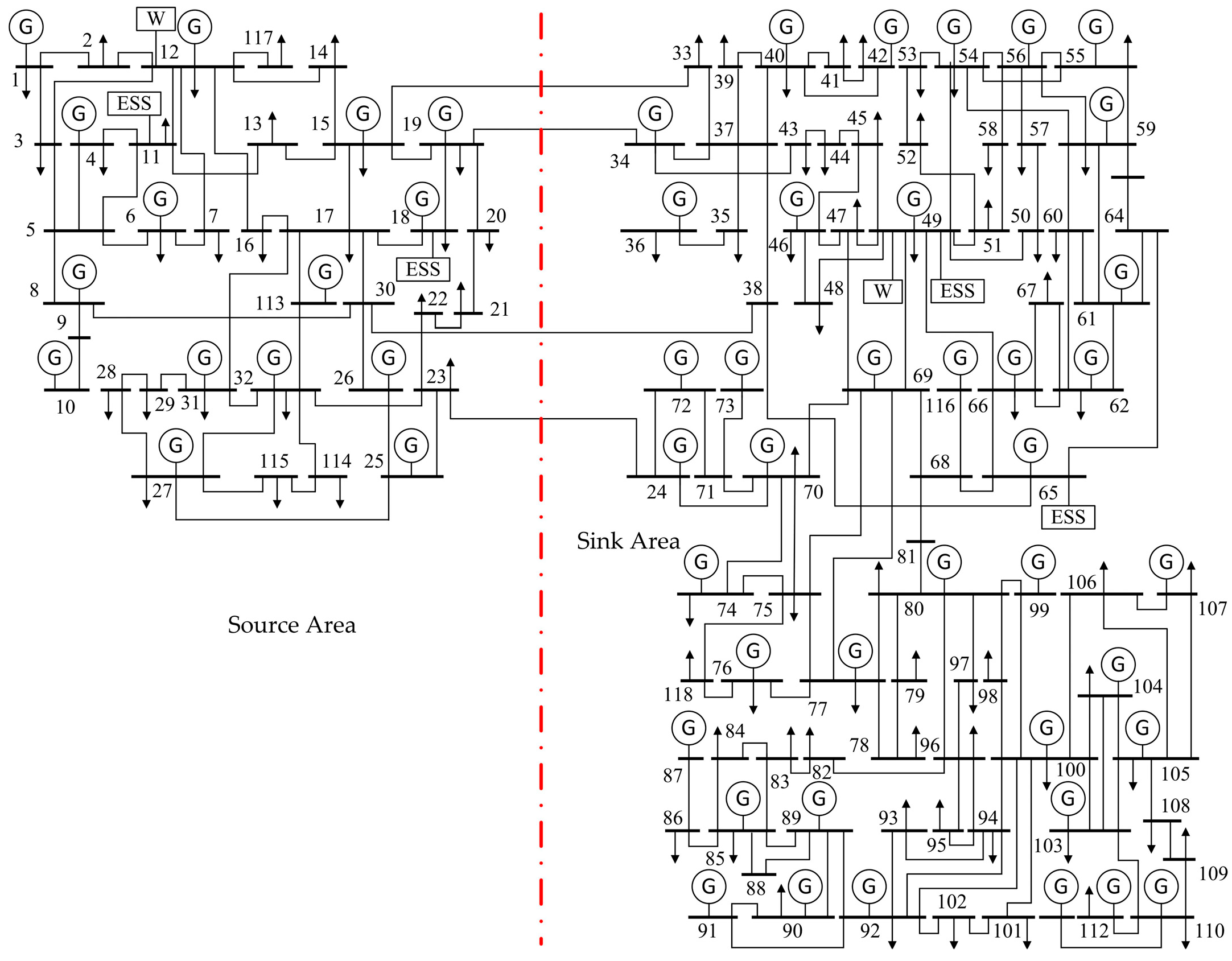
This section extends the case analysis to the IEEE 118-bus system. The partitioned system structure is illustrated in Figure 9. Two wind farms and four energy storage stations are integrated into this system. The wind farm in the sink area includes 15 wind turbines with an installed capacity of 2 MW each, while that in the source area includes 30 wind turbines. Each energy storage station is designed with a power capacity of 200 MW and an energy capacity of 1600 MWh. The remaining parameters of this case study are referenced from the reference [31].

Figure 10 presents the ATC variation over time in this case study. During the early hours (0:00–7:00), when electricity demand is low, there are minimal existing commitments, leaving ample transmission capacity available. As the day progresses, especially between 8:00–19:00, the load demand increases, leading to an increase in the system’s maximum transfer capacity, which remains nearly constant during this period. At the same time, inter-regional power transfers and generation output in the source area increase, leading to a significant reduction in ATC, especially between 16:00 and 18:00, when ATC becomes very small due to the high power transmission requirements. Finally, as the demand decreases in the late evening (20:00–24:00), the existing commitments shrink, and the ATC increases again, demonstrating a shift to lower transmission usage. maximum transferable power.

The results indicate that in regions with high wind power penetration, both the risk parameters and the correlation of wind power forecast errors affect inter-regional ATC assessment. Therefore, ISOs can adjust the risk parameters according to their risk preferences and account for wind farm output correlations to ensure more accurate ATC evaluations.

6. Conclusions

This paper proposes a distributed probabilistic inter-regional ATC assessment framework. Wind power uncertainty is modeled by incorporating spatiotemporal correlations, allowing for the generation of more realistic wind power forecast scenarios. Subsequently, the two-stage optimization model, in which risk-related costs are quantified using CvaR, is proposed for probabilistic ATC assessment. The distributed I-ADMM algorithm is developed to improve computational efficiency while preserving data privacy. Finally, case studies validate that the proposed assessment framework can provide comprehensive, reliable, and secure estimates of inter-regional transfer power capabilities.

The proposed distributed ATC assessment framework offers key advantages in privacy protection and minimizing interference. By only sharing necessary boundary data, it preserves sensitive information that would otherwise be exposed in a centralized system. This approach enables ISOs to make more informed decisions regarding transmission utilization and operational risk management, particularly as renewable energy penetration increases. As power grids become more decentralized with higher renewable energy integration, this distributed ATC calculation method can be further optimized to handle dynamic system changes and enhance grid resilience.

Future research could further analyze the analytical relationship between wind power correlation and ATC capacity, building on the results presented in this study. This could lead to more accurate and efficient ATC assessments in grids with high renewable energy integration.

References

1. Feng, S.; Zhang, X.; Zhang, H.; Ju, L.; Zhang, X. A two-stage bi-level electricity-carbon coordinated optimization model for China’s coal-fired power system considering variable renewable energy bidding. Energy 2024, 312, 133638. [Google Scholar] [CrossRef]
2. Kou, X.; Li, F. Interval optimization for available transfer capability evaluation considering wind power uncertainty. IEEE Trans. Sustain. Energy 2020, 11, 250–259. [Google Scholar] [CrossRef]
3. Zhu, Y.; Dan, Y.; Wang, L.; Zhou, Y.; Wei, W. Integrating Knowledge-Based and Data-Driven Approaches for TTC Assessment in Power Systems with High Renewable Penetration. IEEE Trans. Power Syst. 2024, 39, 5869–5879. [Google Scholar] [CrossRef]
4. Ou, Y.; Singh, C. Assessment of available transfer capability and margins. IEEE Trans. Power Syst. 2002, 17, 463–468. [Google Scholar] [CrossRef]
5. Ejebe, G.C.; Tong, J.; Waight, J.G.; Frame, J.; Wang, X.; Tinney, W. Available transfer capability calculations. IEEE Trans. Power Syst. 1998, 13, 1521–1527. [Google Scholar] [CrossRef]
6. Ejebe, G.C.; Waight, J.G.; Sanots-Nieto, M.; Tinney, W. Fast calculation of linear available transfer capability. IEEE Trans. Power Syst. 2000, 15, 1112–1116. [Google Scholar] [CrossRef]
7. Yu, C.W.; Chung, C.T.; Tse, C.T.; Chung, C.Y. Energy transaction scheduling with interchange capability assessment under open transmission access. Electr. Power Syst. Res. 2023, 67, 59–66. [Google Scholar] [CrossRef]
8. Pan, X.; Xu, G.Y. Available transfer capability calculation considering voltage stability margin. Electr. Power Syst. Res. 2005, 76, 52–57. [Google Scholar] [CrossRef]
9. Cui, Y.; Bie, Z.; Wang, X. Study on calculation of probabilistic available transfer capability. In Proceedings of the International Conference on Power System Technology, Kunming, China, 13–17 October 2002. [Google Scholar] [CrossRef]
10. Mello, J.C.O.; Melo, A.C.G.; Granville, S. Simultaneous transfer capability assessment by combining interior point methods and Monte Carlo simulation. IEEE Trans. Power Syst. 1997, 12, 736–742. [Google Scholar] [CrossRef]
11. Saunders, C.S. Point Estimate Method Addressing Correlated Wind Power for Probabilistic Optimal Power Flow. IEEE Trans. Power Syst. 2014, 29, 1045–1054. [Google Scholar] [CrossRef]
12. Zhang, P.; Lee, S.T. Probabilistic power flow computation using the method of combined cumulants and Gram–Charlier expansion. IEEE Trans. Power Syst. 2004, 19, 676–682. [Google Scholar] [CrossRef]
13. Madadi, S.; Mohammadi-Ivatloo, B.; Tohidi, S. Probabilistic Available Transfer Capability Evaluation Considering Dynamic Line Rating Based on a Sequential Game-Theoretic Approach. IEEE Syst. J. 2022, 16, 891–901. [Google Scholar] [CrossRef]
14. Narain, A.; Srivastava, S.K.; Singh, S.N. Impact of wind power generation on ATC calculation with uncertain equal load. Electr. Eng. 2022, 104, 3–11. [Google Scholar] [CrossRef]
15. Huang, Y.; Ding, T.; Wang, P.; Jia, W.; Ju, C.; He, X.; Zhang, H.; Zhang, Z.; Sun, Y. Linearized AC power flow model based interval total transfer capability evaluation with uncertain renewable energy integration. Int. J. Electr. Power Energy Syst. 2023, 154, 109440. [Google Scholar] [CrossRef]
16. Li, P.; Yu, D.; Yang, M.; Wang, J. Flexible Look-Ahead Dispatch Realized by Robust Optimization Considering CVaR of Wind Power. IEEE Trans. Power Syst. 2018, 33, 5330–5340. [Google Scholar] [CrossRef]
17. Li, X.; Li, J.; Zhang, R.; Li, X.; Wang, M. Probabilistic Available Transfer Capability Assessment in Power System Considering Conditional Value-at-Risk and Correlated Wind Power. Trans. China Electrotech. Soc. 2023, 38, 4162–4177. [Google Scholar] [CrossRef]
18. Liu, J.; Chu, C. Iterative Distributed Algorithms for Real-Time Available Transfer Capability Assessment of Multiarea Power Systems. IEEE Trans. Smart Grid 2018, 6, 2569–2578. [Google Scholar] [CrossRef]
19. Min, L.; Abur, A. Total transfer capability computation for multi-area power systems. IEEE Trans. Power Syst. 2006, 21, 1141–1147. [Google Scholar] [CrossRef]
20. Kou, X.; Li, F.; Dong, J.; Starke, M.; Munk, J.; Xue, Y.; Olama, M.; Zandi, H. A Scalable and Distributed Algorithm for Managing Residential Demand Response Programs Using Alternating Direction Method of Multipliers (ADMM). IEEE Trans. Smart Grid 2020, 11, 4871–4882. [Google Scholar] [CrossRef]
21. Erseghe, T. Distributed Optimal Power Flow Using ADMM. IEEE Trans. Power Syst. 2014, 29, 2370–2380. [Google Scholar] [CrossRef]
22. Aguado, J.A.; Paredes, A. Coordinated and decentralized trading of flexibility products in Inter-DSO Local Electricity Markets via ADMM. Appl. Energy 2023, 337, 120893. [Google Scholar] [CrossRef]
23. Teo, J.C.; Yao, L. Aggregated scheduling of household and public loads with different characteristics in a single-building energy community. J. Build. Eng. 2025, 109, 113032. [Google Scholar] [CrossRef]
24. Zhang, T.; Zhu, Q. Dynamic Differential Privacy for ADMM-Based Distributed Classification Learning. IEEE Trans. Inf. Forensics Secur. 2017, 12, 172–187. [Google Scholar] [CrossRef]
25. Yao, Y.; Wang, Z.; Zhou, P. Privacy-preserving and energy efficient task offloading for collaborative mobile computing in IoT: An ADMM approach. Comput. Secur. 2020, 96, 101886. [Google Scholar] [CrossRef]
26. Zhang, Y.; Lu, Y.; Liu, F.; Li, C.; Gong, Z.; Hu, Z.; Xu, Q. Privacy-preserving and communication-efficient stochastic alternating direction method of multipliers for federated learning. Inf. Sci. 2025, 691, 121641. [Google Scholar] [CrossRef]
27. Li, Z.; Shahidehpour, M.; Wu, W.; Zeng, B.; Zhang, B.; Zheng, W. Decentralized Multiarea Robust Generation Unit and Tie-Line Scheduling Under Wind Power Uncertainty. IEEE Trans. Sustain. Energy 2015, 6, 1377–1388. [Google Scholar] [CrossRef]
28. Yan, M.; Ai, X.; Wen, J.; He, Y.; Zhang, Y. Decentralized Optimization for Multi-Area Optimal Transmission Switching via Iterative ADMM. In Proceedings of the 2018 IEEE Power & Energy Society General Meeting (PESGM), Portland, OR, USA, 5–10 August 2018. [Google Scholar] [CrossRef]
29. Carrion, M.; Philpott, A.B.; Conejo, A.J.; Arroyo, J.M. A stochastic programming approach to electric energy procurement for large consumers. IEEE Trans. Power Syst. 2007, 22, 744–754. [Google Scholar] [CrossRef]
30. Mhanna, S.; Verbič, G.; Chapman, A.C. Adaptive ADMM for Distributed AC Optimal Power Flow. IEEE Trans. Power Syst. 2019, 34, 2025–2035. [Google Scholar] [CrossRef]
31. Matpower User Manual. Available online: https://matpower.org/docs/MATPOWER-manual-7.0.pdf (accessed on 3 August 2020).
Figure 1. Flowchart of the probabilistic ATC assessment procedure.
Mathematics 13 03197 g001
Figure 2. Wind speed and power output with spatiotemporal correlation. (a) the wind speeds between different wind farms. (b) the wind speeds of different turbines within the same farm. (c) the wind speed predictions of wind turbine 1 under different scenarios, where the colored curves represent different scenarios. (d) the power output predictions of wind turbine 1 under different scenarios, where the colored curves represent different scenarios.
Mathematics 13 03197 g002
Figure 3. Topology of Two-area 12-bus System. The letter ‘G’ denotes generators, ‘W’ denotes wind farms, and ‘ESS’ denotes energy storage stations. Arrows denote loads. The numbers denote bus index. The red dashed line divides the system into the source area and the sink area.
Mathematics 13 03197 g003
Figure 4. ATC time variation and transmitted power comparison in 12-bus system.
Mathematics 13 03197 g004
Figure 5. Impact of the confidence level.
Mathematics 13 03197 g005
Figure 6. Impact of the risk factor.
Mathematics 13 03197 g006
Figure 7. Topology of the IEEE 39-bus System. The letter ‘G’ denotes generators, ‘W’ denotes wind farms, and ‘ESS’ denotes energy storage stations. Arrows denote loads. The numbers denote bus index. The red dashed line divides the system into the source area and the sink area.
Mathematics 13 03197 g007
Figure 8. Expected probabilistic ATC and total generation cost under different wind speed correlations. (a) Total generation cost under different wind speed correlations and risk factors. (b) Expected probabilistic ATC under different wind speed correlations and risk factors.
Mathematics 13 03197 g008
Figure 9. Topology of the IEEE 118-bus System. The letter ‘G’ denotes generators, ‘W’ denotes wind farms, and ‘ESS’ denotes energy storage stations. Arrows denote loads. The numbers denote bus index. The red dashed line divides the system into the source area and the sink area.
Mathematics 13 03197 g009
Figure 10. ATC time variation and transmitted power comparison in 118-bus system.
Mathematics 13 03197 g010
Disclaimer/Publisher’s Note: The statements, opinions and data contained in all publications are solely those of the individual author(s) and contributor(s) and not of MDPI and/or the editor(s). MDPI and/or the editor(s) disclaim responsibility for any injury to people or property resulting from any ideas, methods, instructions or products referred to in the content.