Federated Reinforcement Learning with Hybrid Optimization for Secure and Reliable Data Transmission in Wireless Sensor Networks (WSNs)

Abstract

Wireless Sensor Networks (WSNs) consist of numerous battery-powered sensor nodes that operate with limited energy, computation, and communication capabilities. Designing routing strategies that are both energy-efficient and attack-resilient is essential for extending network lifetime and ensuring secure data delivery. This paper proposes Adaptive Federated Reinforcement Learning-Hunger Games Search (AFRL-HGS), a Hybrid Routing framework that integrates multiple advanced techniques. At the node level, tabular Q-learning enables each sensor node to act as a reinforcement learning agent, making next-hop decisions based on discretized state features such as residual energy, distance to sink, congestion, path quality, and security. At the network level, Federated Reinforcement Learning (FRL) allows the sink node to aggregate local Q-tables using adaptive, energy- and performance-weighted contributions, with Polyak-based blending to preserve stability. The binary Hunger Games Search (HGS) metaheuristic initializes Cluster Head (CH) selection and routing, providing a well-structured topology that accelerates convergence. Security is enforced as a constraint through a lightweight trust and anomaly detection module, which fuses reliability estimates with residual-based anomaly detection using Exponentially Weighted Moving Average (EWMA) on Round-Trip Time (RTT) and loss metrics. The framework further incorporates energy-accounted control plane operations with dual-format HELLO and hierarchical ADVERTISE/Service-ADVERTISE (SrvADVERTISE) messages to maintain the routing tables. Evaluation is performed in a hybrid testbed using the Graphical Network Simulator-3 (GNS3) for large-scale simulation and Kali Linux for live adversarial traffic injection, ensuring both reproducibility and realism. The proposed AFRL-HGS framework offers a scalable, secure, and energy-efficient routing solution for next-generation WSN deployments.

1. Introduction

Wireless Sensor Networks (WSNs) are made up of large numbers of small, affordable sensor nodes that function with limited energy reserves. These nodes are often placed in remote or difficult environments where they collect information about physical or environmental conditions, such as temperature, humidity, movement, and air quality [1]. The gathered data are then relayed across multiple nodes until they eventually reach a central sink. Each sensor node typically includes a sensing device, a lightweight processor, a communication module, and a battery, all of which limit its processing power, memory, communication range, and overall energy supply [2]. These limitations make it necessary for WSNs to use routing protocols that are efficient, scalable, and able to extend the network’s lifetime. Today, WSN technology is widely used in fields like environmental monitoring, healthcare, industrial automation, agriculture, military applications, and the development of smart cities. However, the decentralized structure and limited resources of these networks create considerable challenges for their design and long-term operation, especially in changing environments [3]. In 2025, most research is focused on improving energy efficiency, ensuring complete area coverage, reducing communication overheads, and enhancing the reliability of routing protocols. Maintaining these networks manually is often impractical, especially in large-scale or hard-to-reach deployments. Therefore, WSNs must be designed to operate autonomously and remain effective over long periods [4].

Table 1. List of abbreviations.

Abbreviation	Full Form
ABC	Artificial Bee Colony
ACO	Ant Colony Optimization
AES	Advanced Encryption Standard
AES-CTR	Advanced Encryption Standard-Counter Mode
AES-GCM	Advanced Encryption Standard-Galois/Counter Mode
AFRL-HGS	Adaptive Federated Reinforcement Learning with Hunger Games Search
BER	Bit Error Rate
BHA	Black Hole Algorithm
BHA-ACO	Black Hole Algorithm-Ant Colony Optimization
CBSO	Chaotic Bird Swarm Optimization
CH	Cluster Head
CIRP	Cluster-based Intelligent Routing Protocol
CP	Constant Power
CS	Cuckoo Search
CSMA/CA	Carrier-Sense Multiple Access with Collision Avoidance
CVSS	Common Vulnerability Scoring System
DBR	Depth-Based Routing Protocol
DECEM	Dynamic Energy-efficient Clustering and Data Aggregation for Efficient Multi-hop Communication
DDoS	Distributed Denial-of-Service
DoS	Denial-of-Service
DQELR	Deep-Q-Network-based Energy- and Delay-Aware Routing Protocol
DQNs	Deep Q Networks
DQN-EQSR	Double Deep-Q-Network-based Efficient Quality of Service Routing
DQIR	Deep-Q-Network-based Intelligent Routing
DTNs	Delay-Tolerant Networks
E2ED	End-to-End Delay
ECE	Expected Energy Consumed
ERE	Expected Remaining Energy
EWMA	Exponentially Weighted Moving Average
FA	Firefly Algorithm
FIFO	First In, First Out
FRL	Federated Reinforcement Learning
GA	Genetic Algorithm
GADA-LEACH	Genetic Algorithm-based Distributed Adaptive Low-Energy Adaptive Clustering Hierarchy Protocol
GAPSO-H	Genetic Algorithm and Particle Swarm Optimization-based Hybrid Routing
GASO	Green Anaconda Skill Optimization
GNS3	Graphical Network Simulator-3
HGS	Hunger Games Search
I-IoT	Intelligent Internet of Things
IDS	Improved Differential Search
IoUT	Internet of Underwater Things
MACs	Message Authentication Codes
MAD	Median Absolute Deviation
NORTH	Node-Optimized Routing Technique for Heterogeneous WSNs
NVD	National Vulnerability Database
ODM	Optimal Data Routing
PDR	Packet Delivery Ratio
PLR	Packet Loss Ratio
PSO	Particle Swarm Optimization
QLFR	Q-Learning-based Localization-Free Routing Protocol
QoS	Quality of Service
QTAR	Q-learning-based Topology-Aware Routing
RFO	Red Fox Optimization
RL	Reinforcement Learning
RPL	Routing Protocol for Low-Power and Lossy Networks
RSSI	Received Signal Strength Indicator
RTT	Round-Trip Time
SDN	Software-Defined Networking
SECRs	security-aware strategies
SNR	Signal-to-Noise Ratio
TCHS	Trust-based Cluster Head Selection
TDMA	Time-Division Multiple Access
TM	Trust Management
WSNs	Wireless Sensor Networks

defines the abbreviations and acronyms used in this paper, supporting the reader’s understanding.

Energy-efficient and attack-resilient routing in WSNs aims to reduce power consumption while making sure that data remain secure and reliable, even when threats are present [5,6]. Since sensor nodes usually run on limited battery power and are often placed where access is difficult, it is important to design routing strategies that save energy and defend against attacks like sinkhole, Sybil, and selective forwarding [7]. Good routing protocols share communication tasks across nodes to prevent batteries from draining too quickly, and they include security features such as trust scoring, anomaly detection, and secure route selection to stop malicious actions. Modern approaches combine energy-efficient routing with methods like machine learning, trust-based decisions, and metaheuristic optimization so the network can adjust to changing conditions [8,9]. For example, nodes with higher energy and stronger trust records are chosen more often for routing, while less reliable nodes are avoided. Clustering and multipath routing are also used to balance network traffic and make the system more robust against attacks or failures [10]. Using these combined techniques is especially valuable in fields like environmental monitoring, military defense, and smart infrastructure, where both network lifespan and security are essential.

In this paper, we propose AFRL-HGS, a security-aware and energy-efficient routing framework for WSNs that tightly couples tabular Q-learning at each node, FRL at the sink, and a binary HGS initializer for CH selection and routing. Nodes operate as RL agents over discretized state features (residual energy, distance to sink, congestion, path quality, and security), learn next-hop decisions with an $\epsilon$-greedy policy, and periodically upload compressed Q-tables. The sink performs adaptive, energy-/return-weighted aggregation and returns a global model that is blended locally via a Polyak update to avoid catastrophic forgetting. A lightweight anomaly/trust module-fed by EWMA residuals of RTT and loss-constrains the action set to security-admissible paths, while the control plane maintains RoutingTableUP/DOWN through dual-format HELLO and hierarchical ADVERTISE/SrvADVERTISE messages, which are all fully accounted for in the radio-energy model. We evaluate AFRL-HGS in a hybrid testbed (GNS3 for repeatable large-scale simulation, Kali Linux for live Denial-of-Service (DoS), spoofing, and sinkhole injection and trace replay). The main contributions are as follows:

• AFRL-HGS architecture: We introduce a Hybrid Routing framework that integrates per-node tabular Q-learning with adaptive FRL aggregation and binary HGS initializer that jointly optimizes Cluster Heads and feasible routes.
• Security as a constraint via trust/anomaly fusion: We design a lightweight link-trust mechanism that fuses smoothed reliability and anomaly flags. Security acts as an admissibility constraint on actions (not as a reward term), decoupling objectives and improving robustness to spoofing, selective forwarding, and sinkhole attacks.
• Energy-accounted control plane and routing tables: We formalize dual-format HELLO (detailed for CH/sink; lightweight for nodes) and hierarchical ADVERTISE/SrvADVERTISE to populate RoutingTableUP/DOWN, with all control traffic explicitly costed in the first-order radio model.
• Adaptive, reliability-aware federated aggregation: Global Q-tables are computed with weights that depend on residual energy and recent episodic return, and are blended locally (Polyak) to mitigate drift and catastrophic forgetting in resource-constrained nodes.

2. Related Studies

Security remains a major challenge in WSNs, along with other concerns such as limited energy, unreliable data, and unstable communication. Figure 1 categorizes attacks into directed and indirect, where directed attacks lead to packet dropping, while undirected attacks result in different misbehaviors [11]. These attacks are generally categorized as either direct or indirect. In direct attacks, adversaries target the Trust Management (TM) system itself, causing poor performance and faulty routing decisions that weaken the network’s overall effectiveness. If the TM process cannot reliably detect malicious nodes, especially during deceptive behaviors like on-off attacks or false feedback, these nodes may be mistakenly trusted to forward data, which leads to higher packet loss [12]. The configuration of TM systems involves several adjustable parameters, such as adaptive trust dynamics, forgetting factors, trust thresholds, reward and penalty systems, trust evaluation intervals, and ways to combine trust values. How well a TM system works depends on how carefully these parameters are tuned for the network’s specific needs and threats. Regardless of the approach, a strong TM solution must be able to withstand basic security threats. The main goal of Trust Management is to identify nodes that cannot be trusted and limit their influence, which improves the overall security and stability of the WSN [13]. For example, if a node starts dropping packets on purpose, its trust score should decrease automatically.

2.1. Security-Aware Routing

Sameer Dixit et al. [14] proposed a cluster-based routing protocol for WSNs that uses both Red Fox Optimization (RFO) and security-aware strategies (SECRs). Their method relies on the RFO algorithm to select the most suitable CHs by considering multiple factors, including trust value, node centrality, residual and initial energy, and the node’s distance to the sink. To secure communication, the protocol uses adaptive Advanced Encryption Standard (AES) encryption. In low-energy situations, it uses Advanced Encryption Standard-Counter (AES-CTR) mode, while in high-threat conditions, it switches to Advanced Encryption Standard-Galois/Counter Mode (AES-GCM). The protocol manages keys through dynamic updates using secure hash functions, and it ensures data integrity with Message Authentication Codes (MACs). The SECR protocol achieves better energy efficiency, longer network lifetime, and greater resistance to Distributed Denial-of-Service (DDoS) attacks compared to existing solutions such as Dynamic Clustering approach for Energy-hole Mitigation (DECEM), Cluster-based Intelligent Routing Protocol (CIRP), Number of cluster nodes (NORTH), Genetic Algorithm and Particle Swarm Optimization-based Hybrid Routing (GAPSO-H), and Genetic Algorithm-based Distributed Adaptive Low-Energy Adaptive Clustering Hierarchy Protocol (GADA-LEACH). However, it assumes that nodes do not move and that the wireless environment is ideal. Its DDoS detection uses a fixed threshold, which can limit its flexibility in changing conditions. The reliance on the RFO algorithm also adds computational complexity, especially as the number of nodes and iterations increases.

Ferhat Arat et al. [15] developed a security-focused Routing Protocol for Low-Power and Lossy Networks (RPL) framework that uses new objective functions based on real-time risk and vulnerability information to guide routing decisions. Their approach combines data from the National Vulnerability Database (NVD) and Common Vulnerability Scoring System (CVSS) to assess risks at both the node and path levels, helping to detect and prevent rank attacks in IoT networks. The method dynamically updates routing paths by isolating nodes that manipulate rank values and favoring routes through low-risk nodes. Key advantages of this technique include better detection of rank attacks, the ability to assess risk at multiple levels, and the use of real-world vulnerability data, all of which make the protocol more secure and adaptable. However, the framework has limitations: it is designed for static network topologies, has not been tested on large networks beyond 200 nodes, and involves higher computational costs due to complex risk calculations and reliance on APIs. Scalability and real-time adaptability in dynamic environments are still open challenges.

D. Karunkuzhali et al. [16] proposed a comprehensive routing method for IoT-enabled WSNs in smart cities. Their two-phase approach first uses Chaotic Bird Swarm Optimization (CBSO) to cluster sensor nodes and Improved Differential Search (IDS) to select trusted CHs. In the next phase, they apply the Optimal Data Routing (ODM) algorithm for efficient paths and use lightweight signcryption for secure data transmission. Compared to benchmark methods, the NS2 simulation results show significant improvements. These include up to 90.8% less energy consumption, 66.8% longer network lifetime, and up to 80.1% lower latency. The approach blends optimization, trust, and lightweight cryptography for secure and adaptive routing. However, its real-world scalability, flexibility, and performance-especially in highly dynamic or diverse smart city environments-remain untested despite strong simulation outcomes.

2.2. Energy-Aware Routing

Sefati, et al. [17] proposed a cluster-based data transmission method for WSNs that uses the Black Hole Algorithm (BHA) to select CHs and Ant Colony Optimization (ACO) for routing between clusters. The BHA selects CHs based on factors like residual energy, buffer size, and distance to the center of the network, while ACO finds efficient multi-hop paths from CHs to the sink. Their approach, tested in MATLAB R2016b, showed better performance than using ACO alone, the Firefly Algorithm (FA), or Cuckoo Search (CS), with improvements in network lifetime, remaining energy, and the number of packets delivered to the sink. The main strength of this method is its ability to balance energy use and extend the network’s life through better CH selection and routing. However, using both metaheuristics increases computational complexity, especially during the setup and routing phases, which can be a drawback in short-term scenarios or small networks.

Sefati et al. [18] introduced a CH selection and routing algorithm for WSNs that uses Software-Defined Networking (SDN) and game theory. Their method features a game-theoretic clustering approach managed by a central SDN controller. CHs are chosen using utility functions that consider positional advantage, throughput, and remaining energy. For regular data, the protocol uses energy-aware routing based on profit estimation from game theory. High-priority data packets are sent through a First In, First Out (FIFO)-based queue. This approach offers several benefits, including better energy balance, higher PDR, longer network lifetime, and adaptability to both small- and large-scale networks, thanks to SDN’s flexibility. However, the method can face limits with real-time responsiveness if the network topology changes rapidly. The use of game-theoretic calculations also adds computational complexity.

P. K. Udayaprasad et al. [19] proposed an energy-efficient routing system for large-scale Intelligent IoT (I-IoT) networks using a distributed SDN-AI framework. Their approach combines three algorithms: Artificial Bee Colony (ABC) for finding the best mobile sink path, Particle Swarm Optimization (PSO) to identify optimal data-gathering points, and Genetic Algorithm (GA) to cluster nodes with different capabilities. The system is deployed on a cloud-based, three-layer SDN architecture and uses a Time-Division Multiple Access (TDMA) sleep/awake schedule for energy-aware routing, dynamic scheduling, and load balancing. Compared to OMS-LB and RM-LB protocols, this method improves data delivery by 95%, reduces energy use by 78%, and extends network lifetime by 63%. However, the reliance on a central SDN controller can introduce latency and create a single point of failure, especially in real-time or adversarial environments. The lack of real-world testing and the assumption that nodes cannot recharge their energy also limit its use in highly dynamic or self-sustaining IoT networks.

2.3. QoS-Aware Routing

Meiyan Zhang et al. [20] proposed the Double deep Network-based Efficient Quality of Service Routing protocol (DQN-EQSR) protocol for the Internet of Underwater Things (IoUT). This method uses two coordinated Deep Q Networks (DQNs): one for selecting relay nodes and another for controlling acoustic communication. The system works with a multi-dimensional state space that includes node and packet information, and it uses a reward function based on energy cost, link quality, End-to-End Delay (E2ED), and packet priority. Thanks to this dual-network design, sensor nodes can adapt their routing strategies in complex underwater environments. DQN-EQSR performs better than protocols such as Depth-Based Routing Protocol (DBR), Deep Q-network-based Intelligent Routing (DQIR), Q-learning-based Localization-Free Routing protocol (QLFR), Q-learning-based Topology-Aware Routing (QTAR), QELAR, and Deep-Q-Network-based Energy- and Delay-Aware Routing Protocol (DQELR) in PDR, residual energy, average delay, and network lifetime. However, the method’s higher computational demands, longer inference time, and need for precise parameter tuning may limit its practicality for resource-constrained underwater nodes, which are common in IoUT systems.

Basma Mostafa et al. [21] improved multi-constrained Quality of Service (QoS) routing in WSNs by enhancing the RPL protocol without changing its core design. They noted that strict QoS path computation is very demanding for sensor nodes, so they proposed an edge-assisted system where edge servers handle complex routing tasks. This method uses algorithms for conflict-free routing, backup link creation, and Pareto-optimal path selection under QoS limits. Their solution preserved far more QoS-compliant nodes in tests and showed strong scalability across various network conditions. The framework is especially useful for real-time, QoS-sensitive WSN applications, supporting dynamic reconfiguration and lightweight monitoring. Future plans include benchmarking against other protocols and expanding to hybrid fog and edge-cloud networks.

Ashapu Bhavani et al. [22] developed the Multi-objective Green Anaconda Skill Optimization (GASO) algorithm for energy and cache-based QoS-aware routing in Delay-Tolerant Networks (DTN) tailored for IoT settings. GASO combines Green Anaconda Optimization and the Skill-Optimization Algorithm to select optimal CHs and routes, optimizing variables like cache ratio, predicted and residual energy, throughput, distance, trust, and delay, while considering realistic energy and mobility models. This approach lowers communication distance, energy use, and delay while increasing throughput and offers strong scalability and resilience to attacks like wormhole and blackhole. However, the hybrid design adds computational complexity, which may affect real-time performance in large or dynamic networks. Its Trust Management is also basic, lacking deep security integration, and practical deployment still faces challenges due to hardware limits and interference.

Table 2. Comparison of recent trust, energy, and QoS-aware routing methods for WSNs.

Author	Proposed Method	Advantages	Disadvantages
Sameer Dixit et al. [14]	Cluster-based routing with Red Fox Optimization (RFO) and security-aware strategies using adaptive AES encryption modes	Improved energy efficiency, longer network lifetime, resistance to DDoS, secure key updates	Assumes static topology, fixed DDoS thresholds, and introduces RFO-related computational overhead
Ferhat Arat et al. [15]	Security-aware RPL with risk-based objective functions using CVSS and NVD data	Better detection of rank attacks, multi-level risk assessment, adaptable to known vulnerabilities	High computational cost, untested on large/dynamic networks, designed for static environments
D. Karunkuzhali et al. [16]	Two-phase method using CBSO for clustering and IDS for CH selection, ODM for path finding	Reduces energy consumption by 90.8%, lowers latency, combines optimization with lightweight cryptography	Lacks real-world testing; uncertain scalability in dynamic smart city environments
Sefati et al. [17]	Cluster-based method using BHA for CH selection and ACO for inter-cluster routing	Better network lifetime and packet delivery, balances energy consumption effectively	Increased complexity due to dual-metaheuristic setup, not optimal for small-scale/short-term scenarios
Sefati et al. [18]	SDN + game theory-based CH selection and energy-aware routing with FIFO queue	Higher PDR, adaptive to various network scales, energy-balanced operation	Complex calculations, possible delays in rapidly changing topologies
P. K. Udayaprasad et al. [19]	Distributed SDN-AI framework using ABC, PSO, and GA for routing, clustering, and mobile sink pathing	95% higher data delivery, 78% less energy use, 63% longer network life	Central controller adds latency and single-point-of-failure risk; assumes non-rechargeable nodes
Meiyan Zhang et al. [20]	Dual DQN-based EQSR protocol for IoUT routing and communication control	Adapts to underwater dynamics, improves PDR, delay, and lifetime compared to DQELR	High computational cost and tuning complexity; unsuitable for low-resource underwater nodes
Basma Mostafa et al. [21]	QoS-enhanced RPL with edge-assisted routing and conflict-free, Pareto-based path selection	Strong scalability, better QoS compliance, supports real-time and dynamic reconfiguration	No direct benchmarking with many protocols yet; deployment in hybrid networks remains open
Ashapu Bhavani et al. [22]	Multi-objective GASO algorithm for QoS-aware routing with energy and trust optimization	Reduces delay and energy use, resists routing attacks, supports scalability	Complex hybrid model, weak Trust Management, hardware deployment barriers remain

presents a comparison of the recent papers discussed, highlighting the advantages and disadvantages of each method.

3. System Model and Assumptions

We consider a distributed WSN with N static sensor nodes uniformly and independently deployed over a 2D region. Each node has limited compute and memory, a short-range half-duplex IEEE 802.15.4 [5] radio with maximum range $R_{max}$, and a finite initial energy budget $E_{\mathrm{init}}$. Nodes communicate via multi-hop forwarding to a single sink by default (extension to multiple sinks is straightforward and does not alter the algorithms). Time is slotted: at each slot, the nodes sense enqueue data, and may forward packets toward the sink [23].

Every node acts as an RL agent that selects its next hop using local state features such as residual energy, distance to the sink, queue/load, and a path security index. Neighbor discovery is performed by lightweight HELLO beacons broadcast every $T_H$ with random jitter; links are retained only if their smoothed reliability exceeds a minimum threshold $L_{min}$. Energy accounting follows the first-order radio model, where transmission, reception, and processing costs directly feed the battery recursion used throughout our simulations and in the energy results [24].

Adversarial conditions are included to stress the routing/learning stack: per round, a subset of paths is corrupted by DoS [25], spoofing, and selective-forwarding effects; we use synthetic traces and live captures to drive loss and jitter anomalies that the trust module converts into behavioral-trust-based updates.

Figure 2 illustrates that each node trains a local Q-table; only the model summaries are sent to the sink for federated aggregation. A binary HGS stage shapes Cluster Heads and parent links to warm-start RL, accelerating convergence and improving energy balance. The anomaly detector continuously updates trust scores, which constrain admissible actions. The overall objective is multi-criteria: minimize energy and delay while maximizing path security.

3.1. Energy and Communication Model

To ensure consistency between the theoretical formulation, the proposed AFRL-HGS method, and the reported results (Figure 3 and performance plots), we adopt the standard first-order radio model to characterize the energy consumption of sensor nodes in WSNs [26].

Each node spends energy when transmitting, receiving, or locally processing packets. The energy required to transmit a k-bit packet over a distance d is:

$$E_{\mathrm{tx}}(k,d)=\left\{\begin{array}{cc}k·E_{\mathrm{elec}}+k·{ϵ}_{\mathrm{fs}}·d^2,\hfill & d<d_0,\hfill \\ k·E_{\mathrm{elec}}+k·{ϵ}_{\mathrm{mp}}·d^4,\hfill & d\ge d_0,\hfill \end{array}\right.$$

(1)

while the energy required to receive a k-bit packet is:

$$E_{\mathrm{rx}}\left(k\right)=k·E_{\mathrm{elec}}.$$

(2)

Here:

• $E_{\mathrm{elec}}$ denotes the per-bit circuitry cost for transmitting or receiving.
• ${ϵ}_{\mathrm{fs}}$ and ${ϵ}_{\mathrm{mp}}$ are the amplifier parameters for the free-space ($d^2$) and multipath ($d^4$) channel models, respectively.
• The threshold distance is $d_0=\sqrt{\frac{{ϵ}_{\mathrm{fs}}}{{ϵ}_{\mathrm{mp}}}}$.

In addition, each node incurs a computational cost for local reinforcement learning updates and anomaly detection. Thus, the residual energy of node i at time t + 1 is updated as:

$$E_i(t+1)=E_i\left(t\right)-\left(E_{\mathrm{tx}}^i(k,d)+E_{\mathrm{rx}}^i\left(k\right)+E_{\mathrm{comp}}^i\right),$$

(3)

where $E_{\mathrm{comp}}^i$ represents per-packet processing overheads such as policy evaluation, Q-learning updates, and trust computation. This term ensures that learning itself is energy-accounted, directly linking the communication model to the AFRL-HGS design.

Nodes transmit at periodic sensing intervals defined by the sensing rate, $\rho$. A node becomes inactive if its residual energy falls below the minimum threshold, $E_{min}$, which directly influences network lifetime.

This model ensures that energy is explicitly coupled with routing and learning. Transmission, reception, and computation costs appear in the reward function, residual energy contributes to federated aggregation, the total energy is a core term of the HGS fitness function, and energy also shapes aggregation weights. Algorithm 1 describes the energy consumption and communication model used in WSNs.

Algorithm 1 Energy consumption and communication model

3.2. Routing Tables in WSN

In WSNs, routing tables are essential for ensuring efficient, reliable, and energy-aware communication, which becomes even more critical in large-scale or dynamic networks [27]. To support the AFRL-HGS framework, two routing tables are maintained at each node: RoutingTableUP for upward communication toward the sink, and RoutingTableDOWN for downward control and advertisement.

Routing Table Up: RoutingTableUP is used for transmitting sensed data and control packets toward the sink. Parent selection is based on two criteria: (i) minimum hop count, and (ii) maximum recorded Signal-to-Noise Ratio (SNR). This dual criterion reduces both energy consumption and packet loss. Parent nodes periodically broadcast HELLO messages containing hop count and link quality; child nodes update RoutingTableUP accordingly. Each entry includes the following:

• dev, dst, m_seqNo, m_iface, m_hops, nextHop, m_lifeTime, m_minSnr.

RoutingTableDOWN: RoutingTableDOWN supports downward communication from sink to nodes. It is populated from sink-initiated advertisement messages, which are relayed and extended hop-by-hop. Unlike the UP table, the DOWN direction relies only on hop count, since the sink lacks direct SNR information about child links. Thus, m_minSnr is omitted. Each entry includes the following:

• dev, dst, m_seqNo, m_iface, m_hops, nextHop, m_lifeTime.

3.3. HELLO Messages: Structure, Functionality, and Generation in WSNs

HELLO messages are essential for neighbor discovery and route maintenance in WSN routing protocols [28]. To reduce energy overhead, an adaptive broadcast strategy is used: only sink nodes and those with at least one valid upward route transmit HELLO messages. Each HELLO message carries routing metadata including hop count, residual energy, and minimum SNR of the forwarding link. These fields are directly consumed by the following:

• RoutingTableUP: updated with parent candidates based on hop count and SNR.
• RL state space: residual energy and distance metrics are discretized into state features (Step 3).
• Trust evaluation: anomaly and reliability scores are initialized using the reported SNR values (Step 4).

Because HELLO messages are lightweight, they impose minimal energy cost on low-power nodes. The adaptive broadcast interval and hop-limit policy ensure scalability and efficient use of bandwidth, which contributes directly to the observed improvements in Packet Delivery Ratio, Packet Loss Ratio, and End-to-End Delay reported. Algorithm 2 presents the routing table management mechanism for the WSN.

Algorithm 2 Routing table management in WSN

3.4. HELLO Messages: Detailed Format and Role in WSN Routing

Figure 4 shows two formats for HELLO messages in WSNs. One is a lightweight version for sensor nodes with limited energy (Figure 4b). The other is a detailed version used by CHs or sink nodes (see Figure 4a).

The detailed HELLO format (Figure 4a) includes the following fields:

• RecordType (1 byte): Identifies the message as a HELLO message.
• RecordVersion (2 bytes): Indicates the protocol version.
• RecordLength (2 bytes): Total length of the message.
• HandshakeType (1 byte): Shows the operation type, such as update or discovery.
• MessageLength (3 bytes): Size of the message payload.
• MessageVersion (2 bytes): Version number for the HELLO message.
• Random (32 bytes): Contains a nonce to prevent replay attacks.
• SessionIDLength (1 byte): Length of the session ID.
• SessionID: Unique session identifier (variable length).
• CipherSuitesLength (2 bytes): Number of supported encryption algorithms.
• CipherSuites (variable): List of supported encryption methods.
• CompressionMethodsLength (1 byte): Number of supported compression methods.
• CompressionMethods (variable): List of compression methods.
• ExtensionsLength (2 bytes): Total length of the extension section.
• Extensions (variable): Modular extension blocks, each containing:

  –

  ExtensionType (2 bytes): Type of extension, such as residual energy or SNR threshold.

  –

  ExtensionLength (2 bytes): Size of the extension data.

  –

  ExtensionData (variable): Actual routing or network metric data.

Lightweight HELLO Format: (Figure 4b) This format includes only the essential information for routing, leaving out optional fields like encryption, compression, and extensions. It is designed for simple sensor nodes with limited processing power and memory.

Generation Mechanism: The variable m_helloTimerExpire is a timer that triggers the creation of HELLO messages at regular intervals. Sink nodes always broadcast HELLO messages, but intermediate nodes send them only if they have a valid upward route. When generating a HELLO message, the node includes the following:

• HopCount: The smallest known number of hops to the sink.
• MinSNR: The minimum Signal-to-Noise Ratio for the best route.
• OriginatorAddress: Address of the node that created the message.
• SequenceNumber: Incremented to prevent routing loops.

In more advanced WSN setups, extra fields like SessionID and Extensions can be added. These support session tracking and enable multi-metric routing.

The dual-format design of HELLO messages lets WSNs work well in different environments. Regular sensor nodes use simple HELLO formats to save energy. CHs and sink nodes use more detailed messages for better coordination across the network [28]. This modular approach helps make WSNs more scalable, efficient, and flexible in many deployment scenarios.

3.5. HELLO Message Generation in WSNs

Regular HELLO message generation is important for keeping routing information up to date in WSNs. This process is managed by the m_helloTimerExpire parameter and runs at set intervals, as shown in Figure 5. The steps in the generation process are as follows:

• Node Role Identification: Sink nodes act as the root of the routing hierarchy and always generate HELLO messages. Simple nodes create HELLO messages only if they have at least one valid UP-route entry in their RoutingTableUP.
• Field Initialization: Sink nodes directly set fields like HopCount, MinSNR, OriginatorAddress, and SequenceNumber. Simple nodes fill in these fields based on their best route in RoutingTableUP.
• Broadcasting: After building the HELLO message, the node broadcasts it to neighbors. Each recipient checks if the message offers a better route to the sink and updates its routing table if needed.

3.6. Advertising Messages in WSNs

To maintain routing consistency and scalability, the protocol relies on two types of advertisement messages: ADVERTISE and SrvADVERTISE. These messages ensure that both intra-cluster and inter-cluster routing information is regularly refreshed and distributed across the network [29].

3.6.1. ADVERTISE Messages

Simple nodes generate ADVERTISE messages to inform their parent (Cluster Head or sink) of their presence and availability within the cluster. These messages primarily support the population of downward routes in RoutingTableDOWN. Algorithm 3 describes the processing of ADVERTISE messages. A typical ADVERTISE message includes the following:

• HopCount: Number of hops required to reach the originator.
• OriginatorAddress: Unique address of the node that generated the message.
• SequenceNumber: Incremental identifier to avoid duplication and ensure freshness.

Processing ADVERTISE Messages:   

Algorithm 3 ADVERTISE message processing

3.6.2. SrvADVERTISE Messages

SrvADVERTISE messages extend advertisement to the inter-cluster domain. These are created by sink nodes to advertise their own addresses upward to the server, enabling communication across multiple clusters. Algorithm 4 presents the SrvADVERTISE message processing procedure. Each SrvADVERTISE message contains the following:

• HopCount: Distance from the originating node to the sink.
• OriginatorAddress: Address of the originating node.
• SinkAddress: Address of the sink initiating the message.
• SequenceNumber: Unique identifier for freshness and loop prevention.

Processing SrvADVERTISE Messages:

Algorithm 4 SrvADVERTISE message processing

3.6.3. Advertising Message Generation

Both ADVERTISE and SrvADVERTISE messages are generated periodically to ensure fresh routing information. Algorithm 5 illustrates the generation of advertising messages. Their generation depends on node roles:

Algorithm 5 Advertising message generation

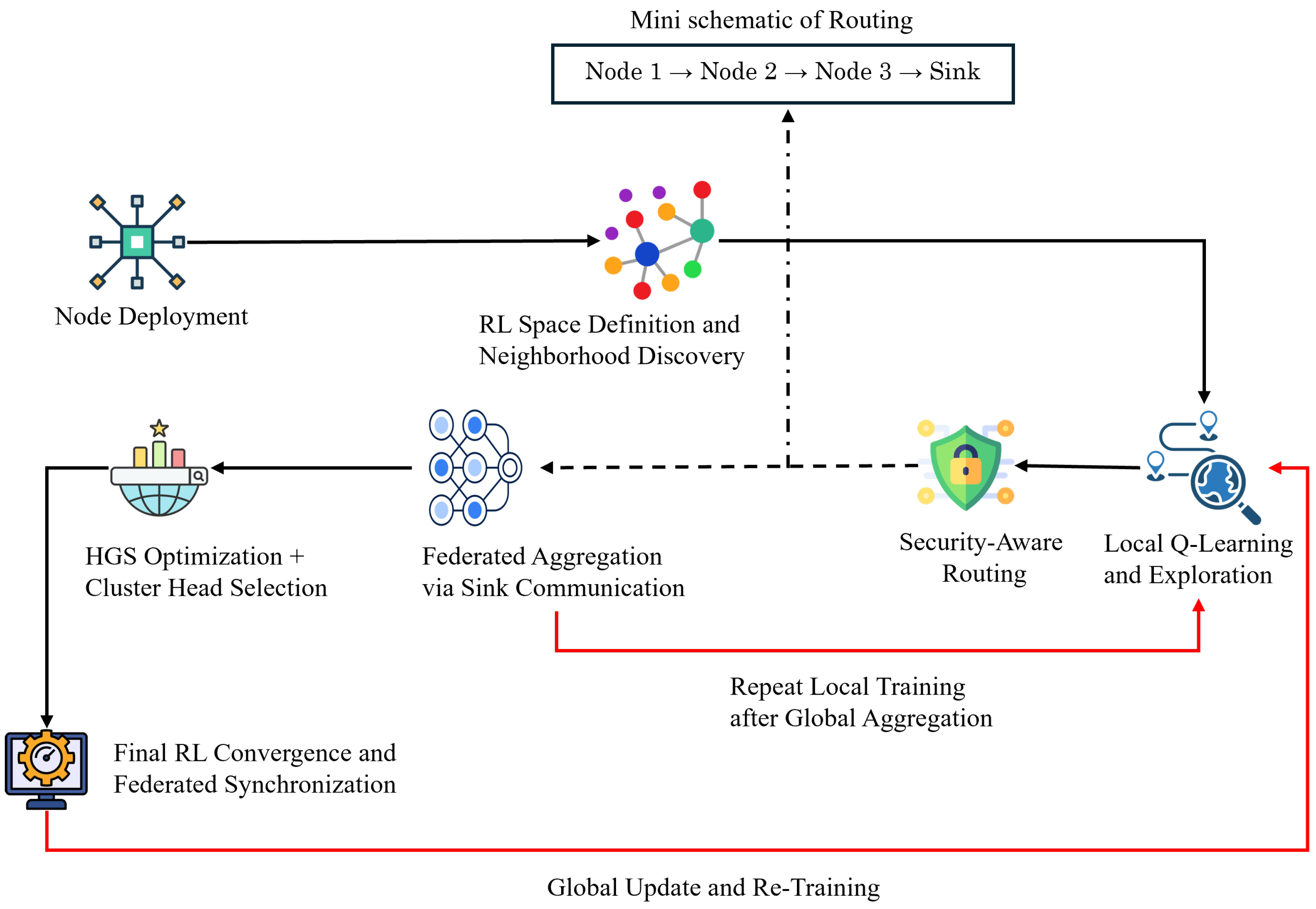
3.7. Proposed Method

Step 1: Initial Modeling of Nodes, Network Topology, and Physical Resources.

We consider a static WSN deployed in a rectangular region $\mathsf{\Omega }\triangleq [0,L_x]\times [0,L_y]\subset {\mathbb{R}}^2$ with a single sink at ${\overrightarrow{x}}_{\mathrm{sink}}\in \mathsf{\Omega }$ (extension to multiple sinks $\mathcal{S}=\{s_1,\dots ,s_{\left|\mathcal{S}\right|}\}$ is straightforward). Nodes are placed i.i.d. uniformly at random in $\mathsf{\Omega }$ and have limited battery, compute, and memory resources.

Node positions and initial energy. Let N be the number of sensor nodes. The position of node i is ${\overrightarrow{x}}_i=\left[\begin{array}{c}{x}_i\\ y_i\end{array}\right]\in \mathsf{\Omega }$, and all nodes start with the same initial energy:

$$\forall i\in \{1,\dots ,N\}:{\overrightarrow{x}}_i\sim \mathcal{U}\left(\mathsf{\Omega }\right),E_i\left(0\right)=E_{\mathrm{init}}.$$

(4)

We assume ideal localization (each node knows ${\overrightarrow{x}}_i$ and the sink broadcasts ${\overrightarrow{x}}_{\mathrm{sink}}$); if localization noise is present, it can be modeled as ${\tilde{\overrightarrow{x}}}_i={\overrightarrow{x}}_i+{\mathit{ϵ}}_i$ with ${\mathit{ϵ}}_i\sim \mathcal{N}(\mathbf{0},{\sigma }_{\mathrm{loc}}^2{\mathbf{I}}_2)$.

Distance and neighborhood. The Euclidean distance between nodes i and j is

$$d_{i,j}\triangleq {∥{\overrightarrow{x}}_i-{\overrightarrow{x}}_j∥}_2,d_{i,\mathrm{sink}}\triangleq {∥{\overrightarrow{x}}_i-{\overrightarrow{x}}_{\mathrm{sink}}∥}_2.$$

(5)

A directed link $i\to j$ is feasible if $d_{i,j}\le R_{max}$, where $R_{max}$ is the PHY-layer communication range.

Radio/energy model. We adopt the first-order radio model with a free-space/multipath crossover distance $d_0$. Let k be the packet size in bits, $E_{\mathrm{elec}}$ the electronics energy per bit (TX/RX), ${ϵ}_{\mathrm{fs}}$ and ${ϵ}_{\mathrm{mp}}$ the amplifier coefficients for free-space ($\eta =2$) and multipath ($\eta =4$) propagation, respectively. The per-packet transmit and receive energies are:

$$\begin{array}{cc}\hfill E^{\mathrm{tx}}(k,d)& =\left\{\begin{array}{cc}{E}_{\mathrm{elec}}k+{ϵ}_{\mathrm{fs}}{d}^{2}k,\hfill & d<d_0,\hfill \\ E_{\mathrm{elec}}k+{ϵ}_{\mathrm{mp}}{d}^{4}k,\hfill & d\ge d_0,\hfill \end{array}\right.\hfill \end{array}$$

(6)

$$\begin{array}{cc}\hfill E^{\mathrm{rx}}\left(k\right)& =E_{\mathrm{elec}}k,\hfill \end{array}$$

(7)

$$\begin{array}{cc}\hfill d_0& \triangleq \sqrt{{\displaystyle \frac{{ϵ}_{\mathrm{fs}}}{{ϵ}_{\mathrm{mp}}}}}.\hfill \end{array}$$

(8)

If on-node processing is non-negligible, we include a per-bit CPU cost $E_{\mathrm{proc}}$ so that the processing energy for k bits is $E^{\mathrm{proc}}\left(k\right)=E_{\mathrm{proc}}k$.

Battery dynamics. Let ${\mathcal{T}}_i\left(t\right)$ and ${\mathcal{R}}_i\left(t\right)$ denote the sets of packets transmitted to and received by node i during slot/epoch t, and let $d_{i,·}$ be the corresponding TX distances. The battery recursion is

$$E_i(t+1)=E_i\left(t\right)-\sum _{p\in {\mathcal{T}}_i\left(t\right)}\left(E^{\mathrm{tx}}(k_p,d_{i,\mathrm{dst}\left(p\right)})+E^{\mathrm{proc}}\left(k_p\right)\right)-\sum _{p\in {\mathcal{R}}_i\left(t\right)}\left(E^{\mathrm{rx}}\left(k_p\right)+E^{\mathrm{proc}}\left(k_p\right)\right),$$

(9)

with node i considered dead when $E_i\left(t\right)\le 0$. Control traffic (e.g., HELLO/ACK, FRL uploads) is accounted for by using (6) and (7) with the appropriate control packet sizes.

Step 2: Neighbor Discovery and Initialization of Communication Metrics.

Each node discovers neighbors and initializes link metrics (distance, reliability, trust primitives) using a lightweight HELLO/ACK procedure over IEEE 802.15.4 Carrier-Sense Multiple Access with Collision Avoidance (CSMA/CA).

MAC/PHY and timing. Time is partitioned in discovery periods of length $T_H$. To reduce collisions, each node transmits one HELLO per period at time $t_i^{\mathrm{HELLO}}=t_0+u_i$ where $u_i\sim \mathcal{U}[0,J_H]$ is a jitter ($0<J_H<T_H$). We use unslotted CSMA/CA with maximum re-transmissions $r_{max}$ for data/ACK frames. Let $k_H$ and $k_A$ be the HELLO and ACK payload sizes (bits).

Control frame formats. Node i broadcasts ${\mathtt{HELLO}}_i=\langle I{D}_i,{\overrightarrow{x}}_i,E_i,t{s}_i\rangle$ ($t{s}_i$ is a local timestamp). Upon reception, neighbor j unicasts ${\mathtt{ACK}}_{j\to i}=\langle I{D}_j,{\overrightarrow{x}}_j,E_j,t{s}_j\rangle$.

Neighbor set and distances. The (directed) neighbor set of i at period t is ${\mathcal{N}}_i\left(t\right)=\{j\ne i\mid \mathrm{ACK}\mathrm{received}\mathrm{from}j\mathrm{in}\mathrm{period}t\}$. Distances follow Step 1: $d_{i,j}\left(t\right)={\parallel {\overrightarrow{x}}_i-{\overrightarrow{x}}_j\parallel }_2$, $d_{i,\mathrm{sink}}\left(t\right)={\parallel {\overrightarrow{x}}_i-{\overrightarrow{x}}_{\mathrm{sink}}\parallel }_2$.

Link reliability estimator. Let $z_{i,j}\left(t\right)\in \{0,1\}$ indicate whether a valid ACK from j to i was received in period t. We maintain both a sliding-window estimator over the last $W_L$ periods and an EWMA:

$$\begin{array}{cc}\hfill L_{i,j}^{\mathrm{win}}\left(t\right)& ={\displaystyle \frac{{\sum }_{\tau =t-W_L+1}^t{z}_{i,j}\left(\tau \right)}{W_L}},\hfill \end{array}$$

(10)

$$\begin{array}{cc}\hfill {\widehat{L}}_{i,j}\left(t\right)& =(1-{\lambda }_L){\widehat{L}}_{i,j}(t-1)+{\lambda }_L{z}_{i,j}\left(t\right),{\widehat{L}}_{i,j}\left(0\right)=L_{i,j}^{\mathrm{win}}\left(0\right),\hfill \end{array}$$

(11)

with ${\lambda }_L\in (0,1]$. A link is considered usable if ${\widehat{L}}_{i,j}\left(t\right)\ge L_{min}$. Neighbors that fail to respond for $W_{\mathrm{miss}}$ consecutive periods are pruned.

RTT and RSSI sampling. For each ACK, node i estimates Round-Trip Time ${\mathrm{RTT}}_{i,j}\left(t\right)=t_{\mathrm{rx}}\left({\mathtt{ACK}}_{j\to i}\right)-t{s}_i$, and records receiver-side RSSI (from the radio), yielding time series $\left\{{\mathrm{RTT}}_{i,j}\left(t\right)\right\}$ and $\left\{{\mathrm{RSSI}}_{i,j}\left(t\right)\right\}$.

Lightweight anomaly detector (for trust primitives). Per link $(i,j)$, define residuals for a generic scalar metric $X\in \{\mathrm{RTT},\mathrm{loss}\}$, where ${\mathrm{loss}}_{i,j}\left(t\right)=1-z_{i,j}\left(t\right)$. Maintain EWMA mean/variance:

$$\begin{array}{cc}\hfill m_X\left(t\right)& =(1-\beta )m_X(t-1)+\beta X\left(t\right),\hfill \end{array}$$

(12)

$$\begin{array}{cc}\hfill v_X\left(t\right)& =(1-\beta )v_X(t-1)+\beta {(X\left(t\right)-m_X(t-1))}^2,\hfill \end{array}$$

(13)

with $\beta \in (0,1]$. The standardized residual is $r_X\left(t\right)={\displaystyle \frac{X\left(t\right)-m_X(t-1)}{\sqrt{v_X(t-1)+\epsilon }}}$ ($\epsilon >0$ small). We flag an anomaly on $(i,j)$ at time t if either $|r_{\mathrm{RTT}}\left(t\right)|>\kappa$ or the windowed loss ${\overline{\mathrm{loss}}}_{i,j}\left(t\right)=1-L_{i,j}^{\mathrm{win}}\left(t\right)$ exceeds ${\tau }_{\mathrm{loss}}$, for at least M consecutive periods. The Boolean flag ${\mathtt{anomaly}}_{i,j}\left(t\right)\in \{0,1\}$ is passed to Step 4’s trust update.

Control plane energy accounting. Let $p_{i\to j}\left(t\right)$ denote the one-shot success probability for $i\to j$ transmissions in period t (estimated by ${\widehat{L}}_{i,j}\left(t\right)$ or PHY metrics). The expected number of transmissions (including CSMA/CA retries, truncated at $r_{max}$) is ${\varphi }_{i\to j}\left(t\right)=\mathbb{E}[\#\mathrm{TX}]={\sum }_{r=1}^{r_{max}}r{p}_{i\to j}\left(t\right){(1-p_{i\to j}\left(t\right))}^{r-1}+r_{max}{(1-p_{i\to j}\left(t\right))}^{r_{max}}$. Assuming a fixed broadcast range $d_i^{\mathrm{bc}}$ for HELLOs, the expected control energy of node i per discovery period is

$$E_i^{\mathrm{ctrl}}\left(t\right)=E^{\mathrm{tx}}(k_H,d_i^{\mathrm{bc}})+\sum _{j\in {\mathcal{N}}_i\left(t\right)}{E}^{\mathrm{rx}}\left(k_A\right)+\sum _{j\in {\mathcal{N}}_i\left(t\right)}{\varphi }_{i\to j}\left(t\right)E^{\mathrm{tx}}(k_A,d_{i,j}\left(t\right)),$$

(14)

which is debited in the battery recursion (Equation (9)).

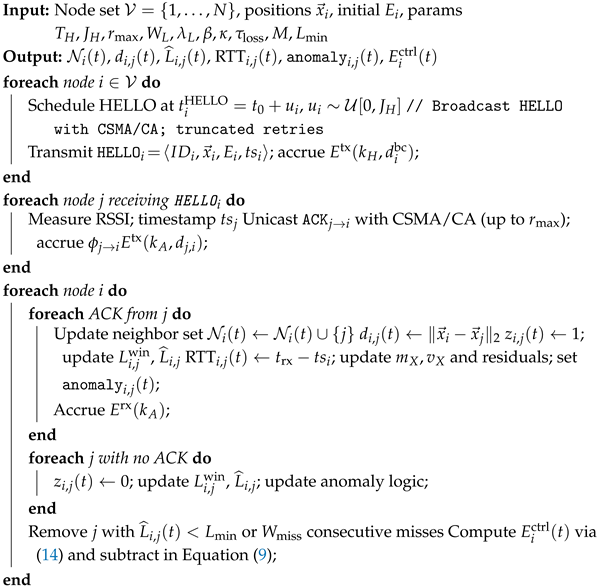
Initialization of trust primitives. Behavioral trust is initialized neutrally: $T_{i,j}^{\mathrm{behav}}\left(0\right)=T_0\in (0,1)$ ($T_0=0.5$) and will be updated in Step 4 using ${\mathtt{anomaly}}_{i,j}\left(t\right)$, ${\widehat{L}}_{i,j}\left(t\right)$, and RTT residuals. Algorithm 6 presents the neighbor discovery and metric initialization procedure.

Step 3: Defining the Reinforcement Learning Space for Network Nodes (Modeling RL Agents).

Each node $n_i$ is modeled as an RL agent that selects its next-hop parent based on local state features. To ensure tractability, continuous state variables are discretized into finite bins, enabling tabular Q-learning.

State space. The state of agent i at time t is represented as:

$$s_t^i=\left[{\mathrm{bin}}_E\left(E_i\left(t\right)\right),{\mathrm{bin}}_d\left(d_{i,\mathrm{sink}}\right),{\mathrm{bin}}_{\sigma }\left({\sigma }_i\left(t\right)\right),{\mathrm{bin}}_q\left(q_i\left(t\right)\right),{\mathrm{bin}}_P\left(P_{i\to \mathrm{sink}}^{\sec }\left(t\right)\right)\right].$$

(15)

• $E_i\left(t\right)$: residual energy of node i, discretized into $B_E$ bins (e.g., 10 uniform bins between 0 and $E_{\mathrm{init}}$).
• $d_{i,\mathrm{sink}}$: distance to sink, discretized into concentric rings $[0,R_1),[R_1,R_2),\dots ,[R_{B_d-1},\infty )$.
• ${\sigma }_i\left(t\right)$: queue congestion index, discretized into $B_{\sigma }$ levels (e.g., $\{\mathrm{empty},\mathrm{low},\mathrm{medium},\mathrm{high}\}$).
• $q_i\left(t\right)$: path quality score (delay/PDR composite), mapped to $B_q$ bins using quantiles or thresholds.
• $P_{i\to \mathrm{sink}}^{\sec }\left(t\right)$: estimated end-to-end security probability from i to the sink, discretized into $B_P$ intervals in $[0,1]$.

Thus, the effective state space is finite with cardinality $|S_i|=B_E·B_d·B_{\sigma }·B_q·B_P$.

Action space. At each step, node i selects one neighbor as the next-hop parent:

$$A_i\left(t\right)=\{a_j\mid j\in {\mathcal{N}}_i\left(t\right),E_j\left(t\right)>E_{min}\}.$$

(16)

Here, ${\mathcal{N}}_i\left(t\right)$ is the neighbor set from Step 2 and $E_{min}$ is the minimum energy threshold for participation.

Reward function. The reward encourages low-energy, low-delay, and secure routing. To avoid mixing different physical units, each term is normalized:

$$r_t^i=-\alpha ·{\displaystyle \frac{E_i^{\mathrm{tx}}\left(t\right)}{E_{max}^{\mathrm{tx}}}}-\beta ·{\displaystyle \frac{D_t^i}{D_{max}}}+\gamma ·{\displaystyle \frac{P_{i\to \mathrm{sink}}^{\sec }\left(t\right)-{\theta }_{\sec }}{1-{\theta }_{\sec }}},$$

(17)

where:

• $E_i^{\mathrm{tx}}\left(t\right)$: transmit energy consumed by node i in epoch t, normalized by a maximum reference $E_{max}^{\mathrm{tx}}$.
• $D_t^i$: End-to-End Delay from node i to sink in epoch t, normalized by a maximum tolerable delay $D_{max}$.
• $P_{i\to \mathrm{sink}}^{\sec }\left(t\right)$: path-level security probability, computed as in Step 4, normalized relative to the threshold ${\theta }_{\sec }$.

The weights $\alpha ,\beta ,\gamma \ge 0$ satisfy $\alpha +\beta +\gamma =1$, balancing the trade-offs among energy, delay, and security.

Algorithm 6 Neighbor discovery and metric initialization (per period of length $T_H$)

Decision policy. Each agent follows an $\epsilon$-greedy policy over its Q-table:

$$\pi (a_t\mid s_t^i)=\left\{\begin{array}{cc}\mathrm{random}(a\in A_i\left(t\right)),\hfill & \mathrm{with}\mathrm{probability}\epsilon ,\hfill \\ arg\underset{a\in A_i\left(t\right)}{max}{Q}_i(s_t^i,a),\hfill & \mathrm{with}\mathrm{probability}1-\epsilon .\hfill \end{array}\right.$$

(18)

The exploration rate $\epsilon$ decays over time, ensuring sufficient exploration initially while converging toward exploitation of high-value routes.

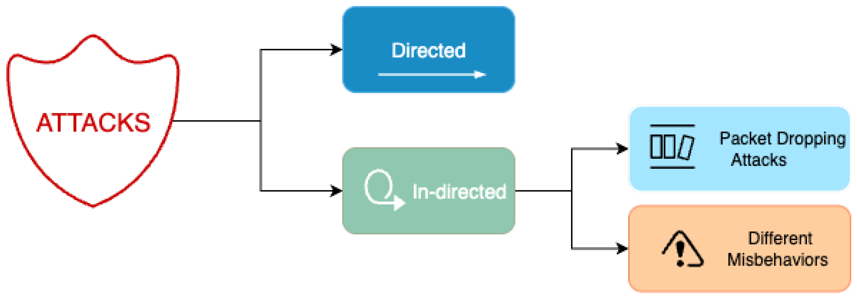
Step 4: Security Evaluation and Path Trustworthiness Assessment.

To ensure that the paths chosen in Step 3 remain resilient against misbehavior and channel anomalies, each node maintains a dynamic trust score per link $(i,j)$.

Hybrid link trust. For each neighbor $j\in {\mathcal{N}}_i\left(t\right)$, node i computes a hybrid link trust:

$$P_{i,j}^{\sec }\left(t\right)=\rho T_{i,j}^{\mathrm{hist}}\left(t\right)+(1-\rho )T_{i,j}^{\mathrm{behav}}\left(t\right),$$

(19)

where:

• $T_{i,j}^{\mathrm{hist}}\left(t\right)\in [0,1]$ is the historical trust, estimated from the smoothed link reliability ${\widehat{L}}_{i,j}\left(t\right)$).
• $T_{i,j}^{\mathrm{behav}}\left(t\right)\in [0,1]$ is the behavioral trust, adapted from anomaly detector outputs (${\mathtt{anomaly}}_{i,j}\left(t\right)$).
• $\rho \in [0,1]$ balances long-term reliability vs. short-term anomaly evidence.

Behavioral trust update. At each discovery period, behavioral trust is updated as:

$$T_{i,j}^{\mathrm{behav}}(t+1)=\left\{\begin{array}{cc}max\left(0,T_{i,j}^{\mathrm{behav}}\left(t\right)-\delta \right),\hfill & \mathrm{if}{\mathtt{anomaly}}_{i,j}\left(t\right)=1,\hfill \\ min\left(1,T_{i,j}^{\mathrm{behav}}\left(t\right)+\mu \right),\hfill & \mathrm{otherwise},\hfill \end{array}\right.$$

(20)

with $\delta \in (0,1]$ the penalty decrement and $\mu \in (0,1]$ the recovery increment.

Path-level security aggregation. To avoid underflow from multiplicative products, path security is aggregated in the log domain:

$$log{P}_{\mathrm{path}}^{\sec }\left(t\right)=\sum _{(u,v)\in p}log{P}_{u,v}^{\sec }\left(t\right),P_{\mathrm{path}}^{\sec }\left(t\right)=exp\left(\frac{1}{\left|p\right|}\sum _{(u,v)\in p}log{P}_{u,v}^{\sec }\left(t\right)\right).$$

(21)

This formulation yields the geometric mean of link trust scores, ensuring longer paths are not unfairly penalized while still reflecting weak links.

Constraint vs. reward. To avoid double counting, we enforce a constraint-only role for security: a candidate path p is admissible if

$$P_{\mathrm{path}}^{\sec }\left(t\right)\ge {\theta }_{\sec },{\theta }_{\sec }\in (0,1),$$

(22)

otherwise, it is excluded from the action set $A_i\left(t\right)$ in Step 3. This ensures that the reward need not include a separate security term, keeping objectives decoupled.

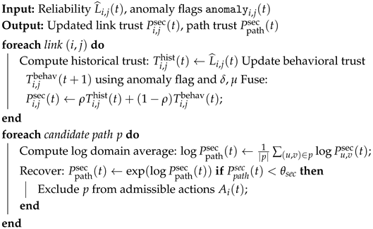
Parameter ranges. Typical values are: $\rho \in [0.3,0.7]$ (balance), $\delta =0.1$–$0.2$ (penalty), $\mu =0.05$–$0.1$ (recovery), and ${\theta }_{\sec }=0.6$–$0.8$ (acceptance threshold). These can be tuned in the simulation setup. Algorithm 7 describes the process of security evaluation and trust updating.

Step 5: Local Q-Learning Model Training for Nodes.

Each node $n_i$ trains its own Q-learning agent over the discretized state/action space defined in Step 3, subject to the admissibility constraints from Step 4. Learning proceeds in episodes, where each episode corresponds to a sequence of packet transmissions and acknowledgments until either the sink is reached or a timeout occurs.

Q-learning update. At each decision epoch t, node i observes its current state $s_t^i\in S_i$, selects an action $a_t\in A_i\left(t\right)$, obtains a normalized reward $r_t^i$ (Equation Step 3), and observes the next state $s_{t+1}^i$. Its Q-table is updated as:

$$Q_i(s_t^i,a_t)\leftarrow Q_i(s_t^i,a_t)+{\eta }_t\left[r_t^i+\gamma \underset{a^{\prime }}{max}{Q}_i(s_{t+1}^i,a^{\prime })-Q_i(s_t^i,a_t)\right],$$

(23)

where:

• ${\eta }_t\in (0,1]$ is the learning rate at epoch t, scheduled to decay as ${\eta }_t={\eta }_0/(1+\zeta t)$ with ${\eta }_0\in [0.1,0.5]$, $\zeta >0$.
• $\gamma \in (0,1)$ is the discount factor, typically $0.8\le \gamma \le 0.95$.
• $r_t^i$ reflects normalized energy, delay, and path security feasibility (from Steps 1–4).

Algorithm 7 Security evaluation and trust update

Exploration-exploitation policy. Node i selects actions using an $\epsilon$-greedy rule:

$$\pi (a_t\mid s_t^i)=\left\{\begin{array}{cc}\mathrm{random}(a\in A_i\left(t\right)),\hfill & \mathrm{with}\mathrm{prob}.{\epsilon }_t,\hfill \\ arg\underset{a\in A_i\left(t\right)}{max}{Q}_i(s_t^i,a),\hfill & \mathrm{with}\mathrm{prob}.1-{\epsilon }_t,\hfill \end{array}\right.$$

(24)

where ${\epsilon }_t$ decays over episodes, e.g., ${\epsilon }_t=max({\epsilon }_{min},{\epsilon }_0·e^{-\kappa t})$, with ${\epsilon }_0\in [0.2,0.3]$, ${\epsilon }_{min}\approx 0.05$.

Stopping criterion and practical convergence. Unlike infinite-horizon Markov Decision Processes (MDPs), WSN agents operate under finite energy budgets and time-varying topologies. Thus, we adopt empirical convergence: training stops after $E_{max}$ episodes or when the Q-values stabilize, i.e., $\parallel Q_i^{\tau +1}-Q_i^{\tau }{\parallel }_{\infty }<{ϵ}_Q$ for M consecutive episodes, with ${ϵ}_Q\ll 1$. This practical stopping rule avoids reliance on ergodicity assumptions that are unrealistic in battery-limited WSNs.

Q-table structure and memory footprint. Each Q-table has dimension $|S_i|\times |A_i|$, where $|S_i|$ is the product of the discretization bins from Step 3, and $|A_i|$ is the number of admissible neighbors. For example, with $B_E=10$, $B_d=5$, $B_{\sigma }=4$, $B_q=5$, $B_P=4$, we obtain $|S_i|=10·5·4·5·4=4000$. If the average neighbor set has $|A_i|=6$, the Q-table has, at most, $\mathrm{24,000}$ entries. With each Q-value stored as a 4-byte float, the per-node memory requirement is $\approx 96$ kB, feasible for constrained sensor platforms with ≥128 kB RAM.

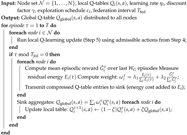
Step 6: Adaptive Federated Aggregation of Q-Learning Models.

To align local policies across the WSN without transmitting raw data, we adopt FRL. Each node $n_i$ periodically uploads a compressed summary of its Q-table after local training, and the sink aggregates these contributions into a global Q-model. This reduces energy overhead compared to centralized training, while ensuring robustness across heterogeneous nodes.

Aggregation model. After local training episode $\tau$, node i has a Q-table $Q_i^{\tau }(s,a)$. The sink aggregates them as:

$$Q_{\mathrm{global}}(s,a)=\sum _{i=1}^N{\omega }_i^{\tau }{Q}_i^{\tau }(s,a),$$

(25)

where ${\omega }_i^{\tau }\ge 0$ and ${\sum }_{i=1}^N{\omega }_i^{\tau }=1$. Thus, nodes with more reliable contributions influence the global model more.

Adaptive weighting. We define ${\omega }_i^{\tau }$ based on both residual energy and local performance:

$${\omega }_i^{\tau }={\lambda }_1·{\displaystyle \frac{E_i\left(\tau \right)}{{\sum }_{j=1}^N{E}_j\left(\tau \right)}}+{\lambda }_2·{\displaystyle \frac{{\overline{G}}_i^{\tau }}{{\sum }_{j=1}^N{\overline{G}}_j^{\tau }}},$$

(26)

where:

• $E_i\left(\tau \right)$: residual energy of node i, consistent with the radio/battery model (Step 1).
• ${\overline{G}}_i^{\tau }$: average return of node i’s policy, i.e., the mean episodic reward over the last $W_G$ episodes (normalized to $[0,1]$).
• ${\lambda }_1,{\lambda }_2\ge 0$: trade-off weights with ${\lambda }_1+{\lambda }_2=1$.

Temporal process. Federated exchange occurs every $T_{\mathrm{fed}}$ local episodes. To reduce communication cost, only nonzero entries or quantized Q-values are transmitted, incurring energy consumption

$$E_i^{\mathrm{FRL}}\left(\tau \right)={\varphi }_{i\to \mathrm{sink}}{E}^{\mathrm{tx}}(k_Q,d_{i,\mathrm{sink}}),$$

where $k_Q$ is the payload size (bits), $d_{i,\mathrm{sink}}$ is the distance to sink, and ${\varphi }_{i\to \mathrm{sink}}$ is the expected re-transmissions.

Local synchronization. Upon receiving the global Q-table, each node blends it with its local table using a Polyak update (to prevent catastrophic forgetting):

$$Q_i^{\tau +1}(s,a)\leftarrow (1-\xi )Q_i^{\tau }(s,a)+\xi Q_{\mathrm{global}}(s,a),\xi \in (0,1).$$

(27)

This ensures stability while gradually aligning local policies with the global one.

Stopping condition. Aggregation continues until either (i) the global Q-values stabilize ($\parallel Q_{\mathrm{global}}^{\tau +1}-Q_{\mathrm{global}}^{\tau }{\parallel }_{\infty }<{ϵ}_{\mathrm{FRL}}$), or (ii) the average number of alive nodes drops below a threshold. Algorithm 8 presents the adaptive federated aggregation of local Q-learning models.

Step 7: Optimization of Clustering and Routing Using Hunger Games Search.

To this end, we apply a binary variant of the HGS algorithm to jointly optimize CH selection and routing paths. The resulting topology minimizes energy consumption, delay, and vulnerability, while ensuring structural feasibility.

Chromosome representation. Each candidate solution is encoded as:

• A binary CH vector $\overrightarrow{z}=[z_1,\dots ,z_N]$ where $z_i=1$ if node i is a CH and $z_i=0$ otherwise.
• A directed binary routing matrix $R\in {\{0,1\}}^{N\times N}$, where $R_{ij}=1$ denotes a parent-child link $i\to j$.

Feasibility constraints. Each solution $(\overrightarrow{z},R)$ must satisfy:

$$\begin{array}{cccc}\hfill & \sum _j{R}_{ij}=1,\hfill & \hfill & \forall i\mathrm{with}{z}_i=0(\mathrm{each}\mathrm{non}\text{-}\mathrm{CH}\mathrm{has}\mathrm{one}\mathrm{parent}),\hfill \end{array}$$

(28)

$$\begin{array}{cccc}\hfill & R_{ij}=0,\hfill & \hfill & \mathrm{if}{d}_{i,j}>R_{max}(\mathrm{within}\mathrm{CH}\mathrm{range}),\hfill \end{array}$$

(29)

$$\begin{array}{cccc}\hfill & R_{ii}=0,\hfill & \hfill & \forall i(\mathrm{no}\mathrm{self}\text{-}\mathrm{links}),\hfill \end{array}$$

(30)

$$\begin{array}{cccc}\hfill & R\mathrm{acyclic},\hfill & \hfill & \mathrm{with}\mathrm{at}\mathrm{least}\mathrm{one}\mathrm{path}\mathrm{to}\mathrm{the}\mathrm{sink},\hfill \end{array}$$

(31)

$$\begin{array}{cccc}\hfill & deg\left(i\right)\le {\Delta }_{max},\hfill & \hfill & \forall i(\max \mathrm{degree}\mathrm{constraint}).\hfill \end{array}$$

(32)

Infeasible candidates are repaired (reassigning orphan nodes) or penalized in the fitness score.

Algorithm 8 Adaptive federated aggregation of Local Q-Learning Models

Fitness function. The objective is to minimize:

$$F(\overrightarrow{z},R)={\lambda }_1{E}_{\mathrm{total}}(\overrightarrow{z},R)+{\lambda }_2{D}_{\mathrm{avg}}(\overrightarrow{z},R)+{\lambda }_3\left(1-P_{\mathrm{secure}}(\overrightarrow{z},R)\right),{\lambda }_1+{\lambda }_2+{\lambda }_3=1.$$

(33)

Metrics are defined as:

• $E_{\mathrm{total}}$: sum of transmit and receive energy for one data collection round:

  $$E_{\mathrm{total}}=\sum _{(i,j):R_{ij}=1}\left(E^{\mathrm{tx}}(k,d_{i,j})+E^{\mathrm{rx}}\left(k\right)\right).$$
• $D_{\mathrm{avg}}$: average End-to-End Delay across all source-sink paths, computed as sum of per-hop delays (including MAC queuing).
• $P_{\mathrm{secure}}$: geometric mean of per-path security probabilities (Step 4):

  $$P_{\mathrm{secure}}={\left(\prod _{p\in \mathcal{P}}{P}_{\mathrm{path}}^{\sec }\left(p\right)\right)}^{1/\left|\mathcal{P}\right|}.$$

HGS update mechanism (binary variant). In the continuous HGS update, candidate solutions evolve via:

$${\tilde{z}}_i^{t+1}=z_i^t+\psi H_i^t(z_{\mathrm{best}}^t-z_i^t)+\delta \mathcal{N}(0,1).$$

To preserve binary encoding, we apply a sigmoid mapping and Bernoulli sampling:

$$P(z_i^{t+1}=1)=\sigma \left({\tilde{z}}_i^{t+1}\right)={\displaystyle \frac{1}{1+exp(-{\tilde{z}}_i^{t+1})}},$$

(34)

then sample $z_i^{t+1}\sim \mathrm{Bernoulli}\left(\sigma \left({\tilde{z}}_i^{t+1}\right)\right)$. This ensures binary Cluster Head assignments.

The hunger factor is computed as:

$$H_i^t={\displaystyle \frac{1}{1+exp(-h_i^t)}},$$

where $h_i^t$ reflects the fitness-induced hunger of solution i.

Step 8: Integrating HGS Output with Reinforcement Learning for Faster Convergence and Structured Stability.

The binary HGS optimization yields an initial Cluster Head assignment ${\overrightarrow{z}}_{\mathrm{opt}}$ and a feasible routing matrix $R_{\mathrm{opt}}$. These outputs are now used to warm-start the Q-learning agents of Step 5, ensuring that training begins from a near-optimal topology rather than from a random policy. This accelerates convergence and improves stability in the early phases of federated aggregation.

Inputs. The initialization procedure uses:

• ${\overrightarrow{z}}_{\mathrm{opt}}\in {\{0,1\}}^N$: optimized CH selection vector.
• $R_{\mathrm{opt}}\in {\{0,1\}}^{N\times N}$: optimized directed routing matrix.
• $\overrightarrow{E}\left(t\right)$: residual energy of all nodes (Step 1).
• $P_i^{\sec }\left(t\right)$: per-node security index (Step 4).

Q-table initialization. For each node i, the Q-table entries corresponding to admissible actions $A_i\left(t\right)$ are initialized as:

$$Q_i(s_0,a_j)=\left\{\begin{array}{cc}{Q}_{\mathrm{init}}^{\mathrm{high}},\hfill & \mathrm{if}{R}_{\mathrm{opt}}[i,j]=1,\hfill \\ Q_{\mathrm{init}}^{\mathrm{low}},\hfill & \mathrm{if}{R}_{\mathrm{opt}}[i,j]=0,\hfill \end{array}\right.$$

(35)

where $Q_{\mathrm{init}}^{\mathrm{high}}>Q_{\mathrm{init}}^{\mathrm{low}}\ge 0$ are bounded constants (e.g., $Q_{\mathrm{init}}^{\mathrm{high}}=1.0$, $Q_{\mathrm{init}}^{\mathrm{low}}=0.1$). This ensures that routes favored by HGS start with higher expected utility.

Policy initialization. The initial decision policy is biased toward the HGS solution:

$${\pi }_0(a\mid s_0)=\left\{\begin{array}{cc}1-{\epsilon }_0,\hfill & \mathrm{if}a=arg\underset{a^{\prime }\in A_i}{max}{Q}_i(s_0,a^{\prime }),\hfill \\ {\epsilon }_0/\left|A_i\right|,\hfill & \mathrm{otherwise},\hfill \end{array}\right.$$

(36)

where ${\epsilon }_0\in [0.1,0.3]$ allows limited exploration from the start. This avoids purely deterministic choices and ensures that suboptimal HGS assignments can still be corrected.

Effect on convergence. With HGS-guided initialization, the number of training episodes needed to reach a near-optimal policy is reduced. There exists ${\tau }_0<{\tau }_{\mathrm{random}}$ such that:

$$\parallel Q_i^{{\tau }_0}-Q_i^{*}{\parallel }_{\infty }<\epsilon ,$$

(37)

meaning that the hybrid HGS-RL process attains an $\epsilon$-close approximation of the optimal Q-function faster than a random-start Q-learning agent. This warm-start effect improves energy efficiency by reducing the number of early, exploratory transmissions that would otherwise consume scarce battery resources.

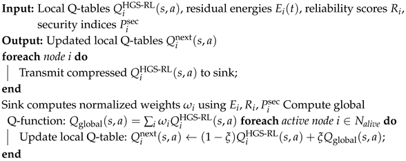
Step 9: Adaptive Re-Aggregation of Learning Policies after HGS-RL Convergence.

After nodes complete their local HGS-guided Q-learning episodes, a second federated aggregation is performed to refine and synchronize policies. This re-aggregation stage ensures that energy-depleted nodes do not dominate decisions, while reinforcing secure and reliable routes across the network.

Inputs. Each node $n_i$ provides:

• Its locally updated Q-table $Q_i^{\mathrm{HGS}\text{-}\mathrm{RL}}(s,a)$, which reflects both RL training and HGS initialization.
• Residual energy $E_i\left(t\right)$.
• Reliability score $R_i$ defined as the Packet Delivery Ratio (PDR) over the last $W_R$ transmissions.
• Security index $P_i^{\sec }$.

Adaptive weighting. The global aggregation weights are computed as:

$${\omega }_i={\lambda }_1·{\displaystyle \frac{E_i\left(t\right)}{{\sum }_j{E}_j\left(t\right)}}+{\lambda }_2·{\displaystyle \frac{R_i}{{\sum }_j{R}_j}}+{\lambda }_3·{\displaystyle \frac{P_i^{\sec }}{{\sum }_j{P}_j^{\sec }}},{\lambda }_1+{\lambda }_2+{\lambda }_3=1,$$

(38)

with ${\sum }_i{\omega }_i=1$. This ensures balanced contributions from energy-rich, reliable, and secure nodes.

Global aggregation. The sink computes the new federated Q-function:

$$Q_{\mathrm{global}}(s,a)=\sum _{i=1}^N{\omega }_i{Q}_i^{\mathrm{HGS}\text{-}\mathrm{RL}}(s,a).$$

(39)

Local synchronization. Instead of overwriting local tables, each node blends the global update into its own Q-table:

$$Q_i^{\mathrm{next}}(s,a)\leftarrow (1-\xi )Q_i^{\mathrm{HGS}\text{-}\mathrm{RL}}(s,a)+\xi Q_{\mathrm{global}}(s,a),\xi \in (0,1).$$

(40)

This prevents catastrophic forgetting and ensures smoother convergence. Algorithm 9 presents the adaptive re-aggregation of HGS-RL Q-tables.

Algorithm 9 Adaptive re-aggregation of HGS-RL Q-tables

4. Dataset and Simulation Setup

The packet source is chosen uniformly at random along the deployment boundary for each simulation run. We compare the proposed AFRL-HGS framework against RFO [14], TCHS [30], BHA-ACO [17], and DQN-EQSR [20].

A hybrid environment is employed:

• GNS3: simulates multi-hop IoT/WSN topology with IEEE 802.15.4 MAC, Q-learning agents, federated aggregation, and HGS optimization.
• Kali Linux (v2023.1): connected via bridged virtual interfaces to inject live adversarial traffic (DoS, spoofing, sinkhole). Captured traces are replayed in GNS3 as packet loss/delay patterns, ensuring realistic perturbations.

Synthetic IoT topology generation: The simulation setup in GNS3 is summarized as

Table 3. IoT topology configuration.

Parameter	Value
Deployment area	$100\times 100$ m2
Nodes	100
Placement	Uniform random
Tx range $R_{max}$	25 m
Initial energy $E_{\mathrm{init}}$	2 J
Packet size	256 B (2048 bits)
Data generation	0.2 pkt/s
Control sizes	HELLO: 256 bits; ACK: 128 bits
HELLO interval $T_H$	5 s (±1 s jitter)
Rounds simulated	1000

.

Radio/Energy model: We adopt the first-order radio model from Step 1:

$$E_{\mathrm{tx}}(k,d)=E_{\mathrm{elec}}k+ϵ\left(d\right)k{d}^{\eta },E_{\mathrm{rx}}\left(k\right)=E_{\mathrm{elec}}k$$

(41)

with $E_{\mathrm{elec}}=50$ nJ/bit, $E_{\mathrm{proc}}=5$ nJ/bit, ${ϵ}_{fs}=10$ pJ/bit/m², ${ϵ}_{mp}=0.0013$ pJ/bit/m⁴, and path-loss exponent $\eta \in \{2,4\}$. The crossover distance is $d_0=\sqrt{{ϵ}_{fs}/{ϵ}_{mp}}$.

Synthetic attacks in GNS3: 10% of routing paths are compromised per round with:

• DoS (ACK suppression, re-transmission flooding).
• Selective forwarding (packet drops).
• Sinkhole (Q-value manipulation).
• Spoofing (false advertisements).

Table 4. Attack Tools and Targets.

Tool	Attack	Layer	Effect in GNS3
hping3	UDP/TCP flooding	Transport	DoS traces (pkt loss, jitter)
scapy	Injection/spoofing	Network	Control plane anomalies
ettercap	ARP poisoning	Link	Traffic redirection
Wireshark	Passive sniffing	All	Ground-truth capture

demonstrates the attack tools and targets used in this paper.

All events are logged to attacktrace.csv (timestamps, node IDs, attack tags, PDR, RTT, Q-deltas).

Table 5. RL and HGS parameters.

Parameter	Value
RL algorithm	Tabular Q-learning + FRL
Learning rate ${\eta }_t$	${\eta }_0=0.2$, decay ${\eta }_t={\eta }_0/(1+0.001t)$
Discount factor $\gamma$	0.9
Exploration ${\epsilon }_t$	${\epsilon }_0=0.25\to {\epsilon }_{min}=0.05$ (exp decay)
Federation interval $T_{\mathrm{fed}}$	50 episodes
FRL blend factor $\xi$	0.2 (Polyak update)
Performance window $W_G$	20 episodes
HGS population/iterations	50/100
Binarization	Sigmoid + Bernoulli
Reward weights $({\lambda }_1,{\lambda }_2,{\lambda }_3)$	(0.4, 0.3, 0.3)
Security threshold ${\theta }_{\sec }$	0.7
Trust parameters	$\rho =0.5$, $\delta =0.1$, $\mu =0.05$
Reliability window $W_L$	10 (EWMA, ${\lambda }_L=0.2$)

demonstrates the RL and HGS parameters used in this simulation.

Classification performance metrics: To assess the effectiveness of AFRL-HGS under adversarial conditions, we use three widely adopted metrics: Accuracy, F1-score, and a robust Z-score (denoted $Z1$) to capture anomaly sensitivity. Each metric is computed over 10 independent runs, each lasting 100 simulation rounds, with adversarial traces injected as described in Section 4.

Accuracy measures the fraction of correctly classified decisions (secure vs. compromised paths):

$$\mathrm{Accuracy}={\displaystyle \frac{TP+TN}{TP+TN+FP+FN}}.$$

(42)

F1-score balances precision and recall:

$$\mathrm{F}1\text{-}\mathrm{score}={\displaystyle \frac{2·\mathrm{Precision}·\mathrm{Recall}}{\mathrm{Precision}+\mathrm{Recall}}}={\displaystyle \frac{2·TP}{2·TP+FP+FN}}.$$

(43)

Robust Z-score (Z1) quantifies the deviation of error observations from the median, using the Median Absolute Deviation (MAD):

$$Z{1}_i={\displaystyle \frac{0.6745·|X_i-\mathrm{Median}\left(X\right)|}{\mathrm{Median}\left(\right|X_j-\mathrm{Median}\left(X\right)\left|\right)}}.$$

(44)

Here $X_i$ is the deviation score of observation i (packet loss or Q-value drift). Lower $Z1$ indicates that routing behavior remains close to the nominal median even under attacks, i.e., stronger anomaly resilience.

The proposed AFRL-HGS framework achieves the highest overall Accuracy and F1-score, while maintaining the lowest $Z1$, thereby demonstrating both strong classification reliability and robustness against adversarial perturbations. In contrast, baseline methods such as DQN-EQSR and BHA-ACO exhibit sharp performance degradation under spoofing and sinkhole attacks, resulting in elevated $Z1$ values (indicating more volatile behavior) and reduced F1-scores. The detailed results are reported in

Table 6. Classification performance.

Method	Accuracy (%)	F1-Score	Z1-Score
Proposed (AFRL-HGS)	98.1	0.962	1.12
RFO	94.5	0.924	1.46
TCHS	93.0	0.905	1.55
BHA-ACO	92.2	0.889	1.64
DQN-EQSR	90.0	0.860	1.77

.

4.1. Energy Consumption

We report energy using the first-order radio model from Step 1. The total energy is

$$E_{\mathrm{consumption}}=\sum _{(i,j)\in \mathcal{E}}\left(E^{\mathrm{tx}}(k_{ij},d_{ij})+E^{\mathrm{rx}}\left(k_{ij}\right)\right)+E_{\mathrm{ctrl}}+E_{\mathrm{FRL}},$$

(45)

where $E^{\mathrm{tx}}(k,d)=E_{\mathrm{elec}}k+ϵ\left(d\right)k{d}^{\eta }$, $E^{\mathrm{rx}}\left(k\right)=E_{\mathrm{elec}}k$ (Step 1), $E_{\mathrm{ctrl}}$ accounts for HELLO/ACK control traffic (Equation (14)), and $E_{\mathrm{FRL}}$ accounts for compressed FRL uploads.

Figure 6 compares the proposed method with four existing approaches: RFO, TCHS, BHA-ACO, and DQN-EQSR. The figure shows energy consumption as the number of nodes increases. All methods use more energy as the network size grows from 0 to 100 nodes. However, the proposed approach consistently uses less energy than the others at every network size. DQN-EQSR and BHA-ACO have the highest energy consumption, especially when the network exceeds 60 nodes. AFRL’s adaptive reward shaping explicitly penalizes unnecessary transmissions and balances traffic across Cluster Heads, while HGS optimizes cluster formation to reduce multi-hop relay distance. This dual mechanism lowers per-packet energy cost and extends lifetime.

4.2. Network Lifetime

Network lifetime is the period between the deployment of sensor nodes and the point when the network is no longer operational. Once the first sensor node fails, the network begins to lose coverage, may become fragmented, and more nodes start to go offline.

The estimated network lifetime is defined as:

$$E_{\mathrm{lifetime}}={\displaystyle \frac{0-\mathbb{E}\left[\mathrm{ERE}\right]}{CP+\mathbb{E}\left[\mathrm{ECE}\right]}}$$

(46)

Here, $CP$ is the Constant Power consumption of the network, $\mathbb{E}\left[\mathrm{ERE}\right]$ is the Expected Remaining Energy after processing, and $\mathbb{E}\left[\mathrm{ECE}\right]$ is the Expected Energy Consumed for data communication per unit of time. The initial, non-rechargeable energy budget is denoted by 0. Traditional methods generally result in a shorter network lifetime compared to the proposed approach.

Figure 7 shows how network lifetime (measured in rounds) changes as the number of nodes increases from 0 to 100. The proposed method keeps the network alive longer at every network size and consistently outperforms RFO, TCHS, BHA-ACO, and DQN-EQSR, while all approaches experience a decrease in network lifetime as more nodes are added mainly due to higher energy use and communication overhead the proposed strategy declines more slowly. This suggests better load balancing and energy management. In contrast, BHA-ACO and DQN-EQSR have the shortest network lifetimes, especially when the network exceeds 60 nodes.

4.3. Packet Delivery Ratio

The cluster-based routing strategy builds routes using the shortest paths and prioritizes CHs with higher residual energy. This approach reduces the number of packet re-transmissions and energy consumption, while also making packet forwarding more reliable and efficient. Simulation results show that the PDR usually decreases as the number of nodes increases. The mathematical definition of PDR is:

$$\mathrm{PDR}={\displaystyle \frac{\mathrm{Total}\mathrm{number}\mathrm{of}\mathrm{data}\mathrm{packets}\mathrm{received}\mathrm{by}\mathrm{the}\mathrm{receiver}}{\mathrm{Total}\mathrm{number}\mathrm{of}\mathrm{data}\mathrm{packets}\mathrm{transmitted}\mathrm{by}\mathrm{the}\mathrm{transmitter}}}$$

(47)

A higher PDR means that data is transferred more reliably across the network.

Figure 8 shows the PDR as a percentage versus network size, with the number of nodes ranging from 10 to 100. The proposed method keeps the PDR close to 99% even as the network grows, achieving the best results across all node densities. In contrast, as the number of nodes increases, the PDR of the other methods RFO, TCHS, BHA-ACO, and DQN-EQSR especially drops noticeably. This means that data delivery becomes less reliable when the network is congested or under scalability stress. DQN-EQSR performs the worst, with its PDR dropping below 95% at 100 nodes. These findings demonstrate that the proposed method can maintain high Accuracy in data delivery, even in large and crowded networks. The security constraint ensures that only reliable and authenticated paths are chosen, reducing packet drops from malicious or unstable nodes. At the same time, the HGS optimization avoids bottlenecks by distributing load, improving reliability.

4.4. End-to-End Delay (E2ED)

The average per-packet delay is

$$\mathrm{E}2\mathrm{ED}={\displaystyle \frac{1}{P}}\sum _{i=1}^P\left(t_i^{\mathrm{received}}-t_i^{\mathrm{sent}}\right),$$

(48)

with P successfully delivered packets. As network size increases, E2ED rises due to longer paths and higher contention. Figure 9 shows the packet drop ratio as the network size increases from 10 to 100 nodes. The packet drop ratio measures the percentage of packets that are not delivered successfully, so higher values mean worse performance. The proposed method consistently achieves the lowest packet drop ratio across all network sizes, showing its reliability and ability to maintain data integrity as the network grows. In contrast, DQN-EQSR and BHA-ACO have the highest drop ratios, both above 5% at 100 nodes. The FRL agent learns to prioritize next-hops with higher SNR and lower hop count. This reduces re-transmissions and queue buildup, thereby lowering delay compared to static schemes.

4.5. Packet Loss Ratio (PLR)

We use the identity $\mathrm{PLR}=1-\mathrm{PDR}$. Accordingly, Figure 10 mirrors the trend in Figure 8. For example, at $N=100$ the proposed method attains $\mathrm{PDR}\approx 98\%$; therefore, $\mathrm{PLR}\approx 2\%$, which is the lowest among all the methods. Figure 10 shows the PLR for different routing strategies as a percentage, based on network size. All methods see an increase in PLR as the number of nodes grows from 10 to 100, mostly due to congestion and higher communication costs. However, the proposed method consistently achieves the lowest PLR for all network sizes, showing it can reduce packet loss even in crowded networks. DQN-EQSR and BHA-ACO have the highest loss rates, going above 12% at 100 nodes. This indicates less reliability in larger networks.

4.6. Bit Error Rate

Bit Error Rate (BER) is an important performance metric that measures how accurately data are transferred in WSNs. A lower BER means better signal quality and more reliable data transmission. Factors such as transmission distance, modulation methods, noise, and interference all affect the BER. It is defined as the ratio of the total number of bits transmitted to the number of bits received incorrectly:

$$\mathrm{BER}={\displaystyle \frac{\mathrm{Number}\mathrm{of}\mathrm{erroneous}\mathrm{bits}\mathrm{received}}{\mathrm{Total}\mathrm{number}\mathrm{of}\mathrm{bits}\mathrm{transmitted}}}$$

(49)

Figure 11 shows the BER as a percentage as the network size increases from 10 to 100 nodes. All methods display a downward trend, meaning that data accuracy improves as the network becomes larger. However, the proposed solution consistently achieves the lowest BER at every network size, reducing it from 15% down to just 4% as the network grows. In comparison, DQN-EQSR maintains the highest BER, staying above 8% even at 100 nodes, while BHA-ACO is the second highest. The strong performance of the proposed method shows its ability to provide reliable and error-resistant data transfer.

4.7. Channel Load

We report average per-node channel occupancy

$$C_L^{\mathrm{node}}={\displaystyle \frac{1}{N}}\sum _{i=1}^N{\displaystyle \frac{D_i}{TB}},$$

(50)

where $D_i$ is the number of bits transmitted by node i over interval T and B is the channel bandwidth. Figure 12 shows slightly higher occupancy for AFRL-HGS at small N, stabilizing as N grows, consistent with higher PDR and lower PLR. This can lead to packet loss, collisions, and increased latency. Effective load balancing and congestion control are needed to maintain optimal network performance.

4.8. Computational Complexity Analysis

Let N be the number of nodes, E be the number of links (with $E=O\left(N\right)$ in sparse networks), G be the HGS population size, T be the number of HGS generations until convergence, A be the number of next-hop actions per node, M be the number of participants per FRL round, and d be the parameter dimension communicated per participant. In our setting, d is constant and does not scale with N.

HGS component. Each generation evaluates G candidate solutions. A single fitness evaluation requires a traversal of the network, which costs $O(N+E)$. Therefore, one generation has cost $O\left(G\right(N+E\left)\right)$, and over T generations the HGS search requires

$$O\left(TG(N+E)\right)=\left\{\begin{array}{cc}O\left(TGN\right),\hfill & \mathrm{if}E=O\left(N\right)(\mathrm{sparse}\mathrm{graphs}).\hfill \end{array}\right.$$

Since G and T are typically small constants, this component scales nearly linearly with N in sparse networks.

FRL component (per round). Assume each participant (a network node) performs a single local update per round. Each local step evaluates a maximum over A actions, costing $O\left(A\right)$. Thus, the total local compute is $O\left(MA\right)$. The server aggregates M parameter vectors of dimension d, costing $O\left(Md\right)=O\left(M\right)$ for constant d. Uplink communication involves M parameter vectors ($O\left(Md\right)$), while downlink costs $O\left(d\right)$ with broadcast (or $O\left(Md\right)$ if unicast). Hence, the per-round FRL system’s work is

$$O\left(MA\right),$$

with communication $O\left(Md\right)$ uplink $+O\left(d\right)$ broadcast downlink.

Overall complexity. The end-to-end per-cycle system’s work (one HGS run plus one FRL round) is

$$\mathrm{Compute}\text{:}O\left(TG(N+E)+MA\right)=\left\{\begin{array}{cc}O\left(TGN+MA\right),\hfill & (\mathrm{sparse}\mathrm{graphs}).\hfill \end{array}\right.$$

$$\mathrm{Communication}\text{:}O\left(Md\right)\mathrm{uplink}+O\left(d\right)(\mathrm{broadcast}\mathrm{downlink}).$$

Thus, when T, G, and A are bounded, and $M=O\left(N\right)$ or capped, both computation and communication scale in a near-linear manner with N in sparse networks. The comparative complexities of AFRL-HGS and baseline methods are summarized in

Table 7. System work complexity comparison between AFRL-HGS and baseline methods.

Scheme	Complexity
LEACH [31] (cluster setup, typical)	$O\left(N^2\right)$
PEGASIS [32] (chain formation, greedy)	$O\left(N^2\right)$
Centralized Q-learning [33] (per step, N agents)	$O\left(NA\right)$
Secure RL [34] (centralized, privacy-preserving aggregation)	$O(NA+N^2)$
AFRL-HGS (proposed)	$O\left(TG\right(N+E)+MA)$

.

5. Open Issues and Future Work

Although the AFRL-HGS framework brings notable improvements, several open challenges remain in achieving optimal energy efficiency and robust security in WSN routing. These challenges cover algorithmic, architectural, deployment, and performance aspects. This section highlights the main unresolved issues and suggests possible directions for future research:

• Scalability to heterogeneous and ultra-dense networks: The proposed framework has been tested with 100 nodes. Real-world WSNs, especially in smart cities and industrial IoT, may involve thousands of nodes with different capabilities. Future work should explore hierarchical federated architectures or clustered aggregation to scale up without overloading the sink node or causing bottlenecks.
• Support for dynamic topologies and node mobility: AFRL-HGS assumes a static or slowly changing network. Applications like vehicular networks (VANET), wildlife tracking, or mobile asset monitoring need support for dynamic topologies. Routing policies and learning intervals should adapt to mobility to keep performance high.
• Cold-start issue and trust bootstrapping: Initial trust values for unknown nodes are set heuristically, which can slow convergence or create security risks. Approaches like reputation inheritance, behavioral fingerprinting, or knowledge from past deployments may help solve this problem.
• Sturdiness against intelligent and adaptive adversaries: The current approach defends against traditional attacks but may be exposed to adversaries using advanced techniques like mimicking attacks or adversarial RL. Co-evolutionary models or adversarial training could help agents in adapting to smarter threats.
• Energy-aware strategies for attack defense: The architecture focuses on energy-aware routing, but energy-aware attacks are not fully considered. Attackers could target energy limits to force re-clustering or early routing changes. Game-theoretic defense strategies could improve resistance.
• Tailored federated synchronization in real-time: Federated Q-learning reduces centralized data transfer but periodic synchronization still adds overhead and delay. Finding the right balance between sync frequency, speed of convergence, and communication cost is a key challenge, especially for low-bandwidth or delay-tolerant WSNs.
• Opportunities for cross-layer optimization: The current method focuses on network-layer routing. Cross-layer optimization combining MAC scheduling, data compression, or adaptive duty cycling could further improve the energy-security trade-off. Integrated RL across multiple layers is a promising direction.
• Explainability and human trust: As WSNs are used in critical fields like healthcare and environmental safety, routing decisions by learning agents must be explainable. Techniques like explainable RL (XRL) and providing confidence scores or policy traces can boost trust and simplify debugging.
• Integration with fog and edge computing: Currently, aggregation is centralized at the sink. Offloading learning and aggregation to edge or fog nodes could reduce latency and boost fault tolerance. Decentralized federated learning with edge-fog coordination is worth exploring.
• Energy harvesting and hybrid energy models: The AFRL-HGS model assumes static, non-rechargeable nodes. New deployments may use energy harvesting (solar, kinetic, thermal). Routing strategies need to estimate energy availability, adapt to fluctuations, and balance processing load with harvesting efficiency.
• Federated communication security: While federated learning keeps data local, Q-value updates can be intercepted or manipulated. Secure aggregation, differential privacy, or blockchain-based validation could make global model updates more secure.
• Domain adaptation and transfer learning: Many WSN deployments are similar in design. Sharing knowledge (pretrained Q-values or trust matrices) across deployments could save training time and reduce initialization overhead.
• Validation on hardware testbeds: Simulations in GNS3 and adversarial injection via Kali Linux are helpful, but real hardware validation is essential. Testing AFRL-HGS on devices like TelosB, MicaZ, or IoT-LAB under real-world conditions would give a more complete evaluation.
• Multi-server and multi-sink settings: The current model uses a single sink node. In practice, large-scale networks often use multiple sinks or cloud-edge hybrids. Extending AFR-HGS to support multi-sink coordination and federated learning across sinks remains an open challenge.
• Verification of RL-based routing policies: Many WSNs are safety-critical, so learned routing policies must not cause risky situations like partitioning or loops. Future research could use formal verification, such as model checking or theorem proving, to guarantee safe agent behavior.

Once these open challenges are resolved, the AFRL-HGS framework can become more practical for real-world deployments, offering enhanced scalability, interpretability, and robustness beyond academic research.

6. Conclusions

This study introduced AFRL-HGS, a Hybrid Routing method that combines FRL and the HGS algorithm to solve problems with energy efficiency and attack resistance in WSNs. In this approach, each sensor node is modeled as a Q-learning agent, which enables decentralized policy learning through federated aggregation and eliminates the need for centralized raw data exchange. The HGS algorithm further improves early routing quality and speeds up learning convergence by optimizing initial clustering and routing based on objectives like energy use, delay, and path security. The proposed framework also uses dynamic trust evaluation and anomaly detection to identify and isolate malicious nodes, which strengthens the network against threats such as selective forwarding, sinkhole, and spoofing attacks. Simulation results from the hybrid GNS3 and Kali Linux testbed show that AFRL-HGS outperforms existing protocols like RFO, TCHS, BHA-ACO, and DQN-EQSR. It uses less energy, increases network lifetime, improves classification Accuracy and PDR, and is more resilient to attacks.

Future research will focus on adding explainable and secure federated learning, supporting mobile nodes, enabling multi-sink coordination, and adapting to energy-harvesting scenarios. The real-world applicability of the AFRL-HGS framework will also be tested through deployments in diverse IoT settings and on actual hardware testbeds.