Article

A Multi-LiDAR Self-Calibration System Based on Natural Environments and Motion Constraints

1
Hubei Research Center for New Energy & Intelligent Connected Vehicle, Wuhan University of Technology, Luoshi Road, Wuhan 430070, China
2
Hubei Key Laboratory of Advanced Technology for Automotive Components, Wuhan University of Technology, Luoshi Road, Wuhan 430070, China
3
Hubei Collaborative Innovation Center for Automotive Components Technology, Wuhan University of Technology, Luoshi Road, Wuhan 430070, China
4
College of Automotive Engineering, Wuhan University of Technology, Luoshi Road, Wuhan 430070, China
5
Hubei Agricultural Machinery Institute, Hubei University of Technology, Nanli Road, Wuhan 430068, China
6
Commercial Product R&D Institute, Dongfeng Automobile Co., Ltd., Wuhan 430056, China
*
Author to whom correspondence should be addressed.
Mathematics 2025, 13(19), 3181; https://doi.org/10.3390/math13193181 (registering DOI)
Submission received: 12 September 2025 / Revised: 27 September 2025 / Accepted: 28 September 2025 / Published: 4 October 2025
(This article belongs to the Section A: Algebra and Logic)

Abstract

Autonomous commercial vehicles often mount multiple LiDARs to enlarge their field of view, but conventional calibration is labor-intensive and prone to drift during long-term operation. We present an online self-calibration method that combines a ground plane motion constraint with a virtual RGB–D projection, mapping 3D point clouds to 2D feature/depth images to reduce feature extraction cost while preserving 3D structure. Motion consistency across consecutive frames enables a reduced-dimension hand–eye formulation. Within this formulation, the estimation integrates geometric constraints on S E ( 3 ) using Lagrange multiplier aggregation and quasi-Newton refinement. This approach highlights key aspects of identifiability, conditioning, and convergence. An online monitor evaluates plane alignment and LiDAR–INS odometry consistency to detect degradation and trigger recalibration. Tests on a commercial vehicle with six LiDARs and on nuScenes demonstrate accuracy comparable to offline, target-based methods while supporting practical online use. On the vehicle, maximum errors are 6.058 cm (translation) and 4.768° (rotation); on nuScenes, 2.916 cm and 5.386°. The approach streamlines calibration, enables online monitoring, and remains robust in real-world settings.

1. Introduction

With advances in artificial intelligence, drive-by-wire, and energy systems, autonomous driving is being deployed across diverse vehicle platforms. Camera-only perception (e.g., BEV representations) has achieved strong results [1,2,3,4], yet LiDAR remains essential for high-accuracy perception and SLAM under challenging illumination. Multi-sensor fusion thus plays a central role in improving precision and robustness [5,6].
In practice, cost-effective solid-state LiDARs with compact FoV are often combined with mechanical LiDARs: the former densify local regions, while the latter provide broad horizontal coverage. Consumer vehicles commonly mount a single front LiDAR, whereas commercial vehicles (e.g., logistics and sanitation trucks) often require multiple LiDARs to extend the field of view and meet stringent safety requirements [7,8]. Accurate extrinsic calibration—both inter-LiDAR and LiDAR-to-vehicle—is therefore critical, because fusion requires mapping all observations into a common vehicle frame.
The effectiveness of multi-sensor fusion heavily depends on precise sensor synchronization and calibration. Recent advances in sensor synchronization have highlighted the importance of precise time alignment between LiDAR and camera systems for effective data fusion [9]. Hardware-level synchronization approaches, including adaptive trigger signal delay estimation, have shown promise in achieving sub-millisecond precision for autonomous driving applications [9]. Additionally, the integration of LiDAR technology with UAV detection systems has demonstrated the versatility of LiDAR sensors across different platforms and applications [10].
Calibration methods are typically divided into target-based [11,12] and targetless approaches [13,14]. Target-based methods use calibration boards or structured targets to form redundant constraints and solve extrinsics with high accuracy, but they require external devices and are inconvenient for operational fleets. Targetless methods exploit natural environmental structure observed during routine driving. While this approach enables online calibration, it faces uncertainty and complexity that demand robust algorithms. Meanwhile, offline procedures [15,16] achieve high accuracy but cannot adapt to pose changes during operation, whereas online calibration [14,17,18] updates extrinsics in real time to accommodate road-induced and structural variations [19], at the cost of higher computational and real-time demands.
For multi-LiDAR systems, calibration is a high-dimensional, nonlinear estimation problem on S E ( 3 ) with heavy data throughput. Observability can be limited by available motion (e.g., planar motion in road scenarios), and naive formulations suffer from cross-axis coupling, sensitivity to initialization, and lack of reliable evaluation during long-term operation [20,21]. Achieving both efficiency and accuracy—without targets and with limited overlaps—remains challenging.
This paper proposes an online self-calibration method that leverages ground plane motion constraints and a virtual RGB–D projection to reduce problem dimensionality while preserving 3D structure for registration. We combine motion consistent ORB associations (on 2D feature/depth images) with 3D ICP refinement and adopt a stepwise hand–eye formulation that estimates yaw on straight segments and planar translation on curved or compound motion. An online monitor fuses plane alignment and LiDAR–INS odometry consistency to detect drift and trigger recalibration. Experiments on a six-LiDAR commercial vehicle and on nuScenes demonstrate accuracy comparable to target-based baselines and suitability for online deployment.
We formulate multi-LiDAR calibration as constrained estimation on S E ( 3 ) under planar-motion reduction. We aggregate plane parameters using a Lagrange multiplier weighted least-squares scheme and estimate planar translation with continuous-time interpolation and quasi-Newton (BFGS) refinement. The formulation foregrounds identifiability under motion constraints, numerical stability in parameter aggregation, and convergence on reduced variables—issues of broad methodological interest in applied optimization and numerical analysis.

2. Related Work

LiDAR extrinsic calibration is commonly categorized into feature-based and motion-constrained methods. Feature-based approaches rely on calibration targets [12] or salient environmental geometry [22]; motion-constrained approaches couple vehicle motion with scene structure and often integrate odometry and mapping [7,11].

2.1. Feature-Based Methods

Target-based systems (e.g., boards, spheres) provide reliable constraints and high accuracy in controlled settings [11,23], but frequent recalibration is impractical for operational fleets. Targetless feature methods use planes or surface normals extracted from natural scenes to estimate extrinsics through iterative minimization [22,24,25]. They reduce hardware dependence yet remain sensitive to environmental complexity and noise, and typically require additional steps to register sensors to the vehicle frame used by downstream planning and control [26,27,28,29].

2.2. Motion-Constrained Methods

Online methods leverage motion and mapping to estimate extrinsics during operation [30,31,32]. Ground constraints can compensate for limited free motion and improve observability (e.g., LiDAR–IMU calibration) [33], while unified frameworks jointly estimate kinematics, extrinsics, and delays and analyze trajectory effects on accuracy [34]. Hybrid pipelines first obtain motion consistent initialization and then refine with feature alignment [35].
Optimization methods play a crucial role in motion-constrained calibration approaches. Traditional gradient-based methods such as BFGS quasi-Newton optimization [36] provide efficient convergence for well-conditioned problems. However, for complex, non-convex optimization landscapes encountered in multi-sensor calibration, evolutionary algorithms, including genetic algorithms, have shown effectiveness in avoiding local minima and exploring the parameter space more comprehensively [37]. These methods are particularly valuable when dealing with high-dimensional parameter spaces and multiple local optima, which are common in multi-LiDAR calibration scenarios.

2.3. Deep Learning-Based Methods

In recent years, deep learning approaches have emerged as a promising alternative for LiDAR-camera extrinsic calibration [38]. These methods can be broadly categorized into two types: accurate extrinsic parameters estimation (AEPE) and relative extrinsic parameters prediction (REPP) [38]. AEPE methods typically use end-to-end networks to directly regress calibration parameters from sensor data [39,40,41], while REPP methods leverage historical calibration data for parameter prediction [38,42]. From both practical utility and deep learning advantages perspectives, AEPE demonstrates greater practical value due to its end-to-end characteristics and offers unique advantages compared with traditional methods.
AEPE can be further divided into global feature-based and local feature-based methods [38]. Global feature-based methods employ CNN architectures to extract global features from depth maps and RGB images, perform feature matching through correlation layers, and regress extrinsic parameters using MLP networks [43,44,45,46]. These approaches benefit from low dependency on scene structure but may suffer from limited generalization ability and poor interpretability. Local feature-based methods utilize semantic segmentation networks to extract local features such as semantic objects, key points, or edges [35,47,48,49], then perform traditional parameter estimation optimization [50]. While these methods offer better interpretability and robustness, they require sufficient environmental structure and semantic targets.
Despite their advantages, deep learning-based calibration methods face several challenges: (1) limited availability of pre-trained models for depth maps; (2) sensitivity to environmental changes and noise; (3) requirement for large amounts of training data; and (4) computational complexity for real-time applications. Furthermore, most existing methods focus on LiDAR-camera calibration, with relatively few studies addressing multi-LiDAR systems.
Overall, targetless and motion-based approaches enhance practicality for multi-LiDAR systems but still face challenges in robustness, real-time performance, and online evaluation. Our method combines ground plane dimensionality reduction, efficient virtual RGB–D registration, a stepwise hand–eye formulation, and an online monitor to improve robustness under limited overlaps and tilted sensors while detecting drift during long-term operation.

3. Problem Formulation and Overview

We use a commercial sanitation vehicle equipped with a multi-LiDAR setup and a high-precision integrated navigation module (Figure 1). To facilitate reference, we define the vehicle body coordinate system { V } at the center of the vehicle’s rear axle, with the forward direction as the positive Y-axis and the upward direction as the positive Z-axis. Each LiDAR has its own right-handed Cartesian coordinate system { L n } . We assume that the integrated navigation system (GNSS, RTK, and IMU) is calibrated and aligned with the vehicle coordinate system. This means that { I } coincides with { V } . In the following, the coordinates provided by the integrated navigation system are considered as the coordinates of the vehicle coordinate system { V } in the global coordinate system { G } .
The core of the multi-LiDAR calibration problem lies in determining the relationship between each LiDAR’s coordinate system { L i } and the vehicle coordinate system { V } . Specifically, we aim to determine the extrinsic calibration matrix T V L i , which allows us to transform LiDAR measurements to the vehicle coordinate system for further perception tasks:
p V = T V L i p L i ,
where p L i represents a point in the LiDAR coordinate system, and p V represents its corresponding coordinates in the vehicle coordinate system.
By calibrating multiple LiDARs to the vehicle coordinate system { V } , we can indirectly obtain the transformation relationships between each LiDAR, allowing their point clouds to be merged into a unified coordinate system to provide maximum coverage for the perception module:
p L i + 1 = T L i + 1 L i p L i ,
where p L i and p L i + 1 represent the coordinates of a point in LiDAR i and i + 1 , respectively.
As illustrated in Figure 2, our online pipeline comprises three phases:
  • Preprocessing: Where a ground plane assumption reduces motion to planar DoF (fixing t z , roll, and pitch) and yields T L i , 2 L i , 3 ; a virtual RGB–D projection produces 2D feature/depth maps, and ORB with motion consistency filtering provides robust associations that are refined by 3D ICP.
  • Optimization for hand–eye calibration: Optimization for hand–eye calibration, where yaw is estimated from straight segments via motion constraints, and—assuming the INS is aligned to the vehicle frame—planar translation ( t x , t y ) is solved during curved/compound motion via INS–LiDAR consistency.
  • Error evaluation: Error evaluation, which continuously monitors plane-alignment (normal angle and mean offset) and LiDAR–INS odometry discrepancies (translation and rotation); threshold exceedances indicate drift and trigger online recalibration.

4. Preprocessing

In preprocessing, a ground plane constraint reduces motion to planar DoF, and a virtual RGB–D projection turns 3D scans into 2D feature/depth maps that preserve spatial hierarchy while enabling efficient registration. These steps simplify the subsequent hand–eye calibration without sacrificing geometric fidelity.

4.1. Ground Plane Fitting for Motion Dimensionality Reduction

Since most vehicles travel on nearly horizontal roads, the vehicle motion can be reduced to a two-dimensional plane. The aim of the ground fitting process is to determine the extrinsic parameters of the LiDAR sensors with respect to the vehicle body, specifically translation along the Z axis and rotation around the X and Y axes, thus reducing the degrees of freedom (DoF) of the vehicle’s motion. Our method is primarily designed for urban commercial vehicle applications, where near-planar motion is the dominant scenario. While this assumption may limit applicability in complex terrain, it significantly simplifies the calibration process and reduces operational complexity for fleet management.

4.1.1. Point Cloud Acquisition and Ground Plane Estimation

For the n-th point cloud frame P i , n collected by LiDAR i, the ground points are extracted and fitted to a plane using the RANSAC (Random Sample Consensus) algorithm [51]. The estimated ground plane is represented as
f ^ Plane ( i ) : a i x + b i y + c i z + d i = 0
where ( a i , b i , c i ) represent the components of the normal vector of the plane, and d i is the offset from the origin.

4.1.2. Global Plane Parameter Optimization

To robustify plane estimation across frames, we combine framewise RANSAC fits with a residual-weighted least-squares aggregation. This aggregation is performed under a unit-normal constraint. Let ( a i , n , b i , n , c i , n , d i , n ) be the per-frame estimates for LiDAR i at frame n with weight w i , n ; we seek globally consistent ( a i , b i , c i , d i ) by solving [51]:
min a i , b i , c i , d i n = 1 N w i , n ( a i a i , n ) 2 + ( b i b i , n ) 2 + ( c i c i , n ) 2 + ( d i d i , n ) 2 ,
a i 2 + b i 2 + c i 2 = 1 .
Using Lagrange multipliers [52], the constrained objective becomes
L ( a i , b i , c i , d i , λ i ) = n = 1 N w i , n E i , n λ i a i 2 + b i 2 + c i 2 1 ,
with per-frame residual
E i , n = ( a i a i , n ) 2 + ( b i b i , n ) 2 + ( c i c i , n ) 2 + ( d i d i , n ) 2 .
We align each LiDAR’s ground plane to X O Y by rotating its normal vector to [ 0 , 0 , 1 ] T and translating the plane to remove the offset. The rotation is obtained from the axis–angle between normals using Rodrigues’ formula; translation shifts a point on the plane to z = 0 . This yields T L i , 2 L i , 3 that fixes t z and ( α , β ) while preserving scene geometry.
To compute the transformation matrix T L i , 2 L i , 3 , we separate it into rotation and translation. The rotation R L i , 2 L i , 3 aligns the ground normal n i with n X O Y by rotating about axis u i through angle θ i :
n i = [ a i b i c i ] T , n X O Y = [ 0 0 1 ] T , u i = n i × n X O Y n i × n X O Y , θ i = arccos n i · n X O Y
The rotation matrix is then constructed using Rodrigues’ formula [53]:
R L i , 2 L i , 3 = I 3 × 3 + sin ( θ i ) K i + 1 cos ( θ i ) K i 2
where I 3 × 3 is the identity matrix, and K i is the skew-symmetric matrix of the rotation axis u i . If the centroid of the transformed point cloud lies below the X O Y plane after applying T L i , 2 L i , 3 , an additional 180° rotation about either the X or Y axis is applied.
As shown in Figure 3, we selected the rear LiDAR of the experimental vehicle as an example. In the figure, red points represent those below the X O Y plane of coordinate frame { L } , while green points represent those above or on the X O Y plane of coordinate frame { L } .

4.2. Fast Point Cloud Registration Using Virtual Camera Model

To improve registration efficiency and robustness, we employ a virtual RGB–D camera to project 3D point clouds into 2D feature and depth maps after ground alignment. A wide FOV increases spatial context (with distortion trade-offs) but benefits 2D registration.

4.2.1. Virtual Camera Projection

The RGB–D image is generated by projecting a point p = [ a b c ] T in the 3D LiDAR coordinate system into a 2D image coordinate p = [ u v 1 ] T based on the perspective projection principle:
z c u v 1 = f x 0 c x 0 f y c y 0 0 1 R c l t c l 0 1 x y z 1 = M 1 M 2 x y z 1
where M 1 represents the intrinsic parameters of the virtual camera, such as focal length and principal point offsets, and M 2 represents the extrinsic parameters, including the position and orientation of the virtual camera in the point cloud coordinate system. As shown in Figure 4, the point cloud is projected into both a depth image and a feature image using this virtual camera.
To cover the cloud and control accuracy, we set image resolution η (mm/pixel) over extents S x and S y . Intrinsics ( f x , f y , c x , c y ) follow from the chosen FOV and image size, and extrinsics place the virtual camera above the cloud centroid ( C x , C y , C z ) .
To visualize the variation in point cloud intensity, we map the intensity values to a color spectrum within the feature map. Figure 5 compares feature maps for different FOVs. Larger FOV α enhances spatial hierarchy in the 2D map relative to simple Z-axis reduction, despite added distortion.
To address concerns about geometric detail preservation during 3D-to-2D projection, we implement a comprehensive strategy that balances computational efficiency with geometric fidelity. The key challenge lies in selecting appropriate FOV parameters that capture sufficient environmental details while maintaining feature quality for robust matching. When FOV is relatively small (e.g., 30°), the virtual camera operates like a telephoto lens, positioned at higher altitudes to minimize distortion but with limited spatial coverage that primarily captures top-layer point cloud features. Conversely, larger FOVs (e.g., 120°) function like wide-angle lenses, positioned at lower altitudes to capture enhanced spatial hierarchy and more environmental details, though excessive FOV values can introduce perspective distortion and sparse feature distribution that compromise matching accuracy.
For different LiDAR configurations, we adapt FOV settings based on sensor specifications to optimize feature extraction. High-resolution LiDARs (e.g., 128-line) can effectively utilize larger FOVs to capture detailed geometric features, while lower-resolution sensors benefit from smaller FOVs to maintain adequate feature density. The subsequent 3D ICP refinement step serves as a crucial recovery mechanism, restoring geometric details that may be lost during the initial projection phase, thereby ensuring that critical geometric shapes are preserved through our two-stage registration process. This approach allows us to leverage the computational advantages of 2D feature matching while maintaining the geometric accuracy essential for precise calibration.

4.2.2. Feature Map and ORB Matching

We extract ORB features [54,55], match by Hamming distance, then apply motion consistency filtering using slope/length modes with tolerances ε K , ε L to remove outliers (Figure 6). We compute per-pair slopes k i and lengths l i between consecutive matches and keep pairs near the modal values within tolerances.

4.2.3. ICP Refinement

Traditional ICP [56] is sensitive to initialization and noise. We compute a transformation from filtered 2D correspondences and refine it with 3D ICP to obtain the final registration, mitigating sensitivity and improving efficiency.

5. Hand–Eye Calibration

Under planar motion, we adopt a decoupled, stepwise scheme: estimate yaw from straight segments and translation from curved/compound motion. This reduces cross-axis interference and relaxes registration accuracy requirements.

5.1. Yaw from Straight Motion

During straight-line driving, we register adjacent frames to obtain Δ E n + 1 , i n containing Δ R L and Δ p L . We align the translation direction with the vehicle’s + Y to estimate γ V L i .

5.1.1. Motion Direction Extraction

From the translation vector Δ p L , the motion direction unit vector u L is calculated as
u L = Δ p L Δ p L
Since we consider only planar motion, the Z component of the motion is ignored. The rotation of the LiDAR relative to the vehicle body is represented by a rotation matrix R γ V L i around the Z axis:
R γ V L i = cos γ V L i sin γ V L i 0 sin γ V L i cos γ V L i 0 0 0 1
The vehicle’s motion direction in its own coordinate system v V is assumed to be along the positive Y axis:
v V = R γ V L i · v L

5.1.2. Optimization to Determine Yaw Angle

The error function E ( γ V L i ) is defined as the sum of squared differences between the observed and predicted motion directions across all frames during straight-line motion:
E ( γ V L i ) = i = 1 n v V , i R γ V L i · v L , i 2
The yaw angle γ V L i is iteratively updated to minimize this error using a least-squares approach until convergence.

5.2. Translation from Curved/Compound Motion

After estimating yaw, we solve ( t x , t y ) over straight and curved segments. We assume time alignment between INS and LiDAR; when frequencies differ, we apply B-spline interpolation [57] for continuous-time states. During curved motion, LiDAR and GNSS-IMU obey
Δ E t + 1 , I t T I L i = T I L i Δ E t + 1 , L i t
We estimate t X = [ t x t y ] T by minimizing discrepancies between observed LiDAR motion and predictions, using a BFGS quasi-Newton method [36]. To ensure robust convergence and avoid local minima, we adopt a multi-strategy approach. First, we initialize the translation parameters using the yaw-estimated frame as a warm start, leveraging motion consistency from the previous optimization phase to provide a good initial guess. Second, we employ multiple initialization strategies, including temporal consistency from previous frames and small random perturbations, to escape potential local minima. Third, the planar motion constraint inherently reduces the parameter space from 6-DOF to 2-DOF, making the optimization landscape more convex and significantly reducing the likelihood of local minima. Finally, we implement robust convergence criteria that terminate optimization when parameter changes fall below threshold ϵ p a r a m or gradient norms are smaller than threshold ϵ g r a d .

5.3. Combined Extrinsic Parameters

Finally, the extrinsic transformation matrix T V L i between the LiDAR and the vehicle body is obtained by combining the calibration matrices from each phase:
T V L i = T trans t X · R z γ V L i · T L i , 2 L i , 3

6. Precision Evaluation

To ensure accuracy and monitor drift online, we perform a two-stage evaluation.

6.1. Ground Plane Error

After calibration, the ground plane fitting is repeated using the calibrated parameters, and the angle between the fitted plane normal n and the ideal ground plane normal n X Y is calculated:
δ θ = arccos n · n X Y n n X Y
The average angle deviation δ θ ¯ is used to evaluate the rotation accuracy, while the average plane offset d ¯ is used to evaluate the translation accuracy.

6.2. Odometry Consistency Error

The calibrated extrinsic parameters are also evaluated by comparing the estimated odometry from the LiDAR and GNSS-IMU systems. The translation error e t and rotation error e r are defined as
e t = t L ( t ) t I ( t )
e r = arccos trace R L ( t ) T R I ( t ) 1 2
If these errors exceed predefined thresholds, the system triggers a recalibration process to update the extrinsic parameters.

7. Experiments and Results

We validate effectiveness and efficiency via registration and calibration experiments. We compare registration accuracy and runtime against PFH + ICP, FPFH + ICP, and NDT on ground-aligned adjacent frames, benchmark calibration against OpenCalib [23,24] on a commercial vehicle, and evaluate generalization on nuScenes using dataset extrinsics as ground truth.

7.1. Experiment Setup

We use two settings: (i) a commercial sanitation vehicle platform (Figure 1) with six LiDARs for 360° coverage (one 128-line front solid-state unit plus five 32-line mechanical units) and a high-precision integrated navigation module for continuous localization and (ii) the nuScenes dataset for cross-platform evaluation. In addition to the sanitation vehicle shown in Figure 1, we also deployed our algorithm on a water sprinkler truck with the same chassis configuration. Since both vehicles share identical chassis and sensor configurations, we selected one for detailed presentation.
For quantitative metrics, we follow [13]. Rotations are compared via quaternion difference and translations via norms:
E t = t t ^ 2
m = q q ^ 1
E R = atan 2 m x 2 + m y 2 + m z 2 , m w
where t and t ^ denote target and estimated translations, and q and q ^ denote target and estimated rotations; ∗ and 1 denote quaternion multiplication and inversion.

7.2. Registration Methods Comparison

We align adjacent ground-aligned scans to recover motion and apply the same registration in the online calibration pipeline. We compare against classic algorithms to assess effectiveness and runtime. The experimental platform is depicted in Figure 1.
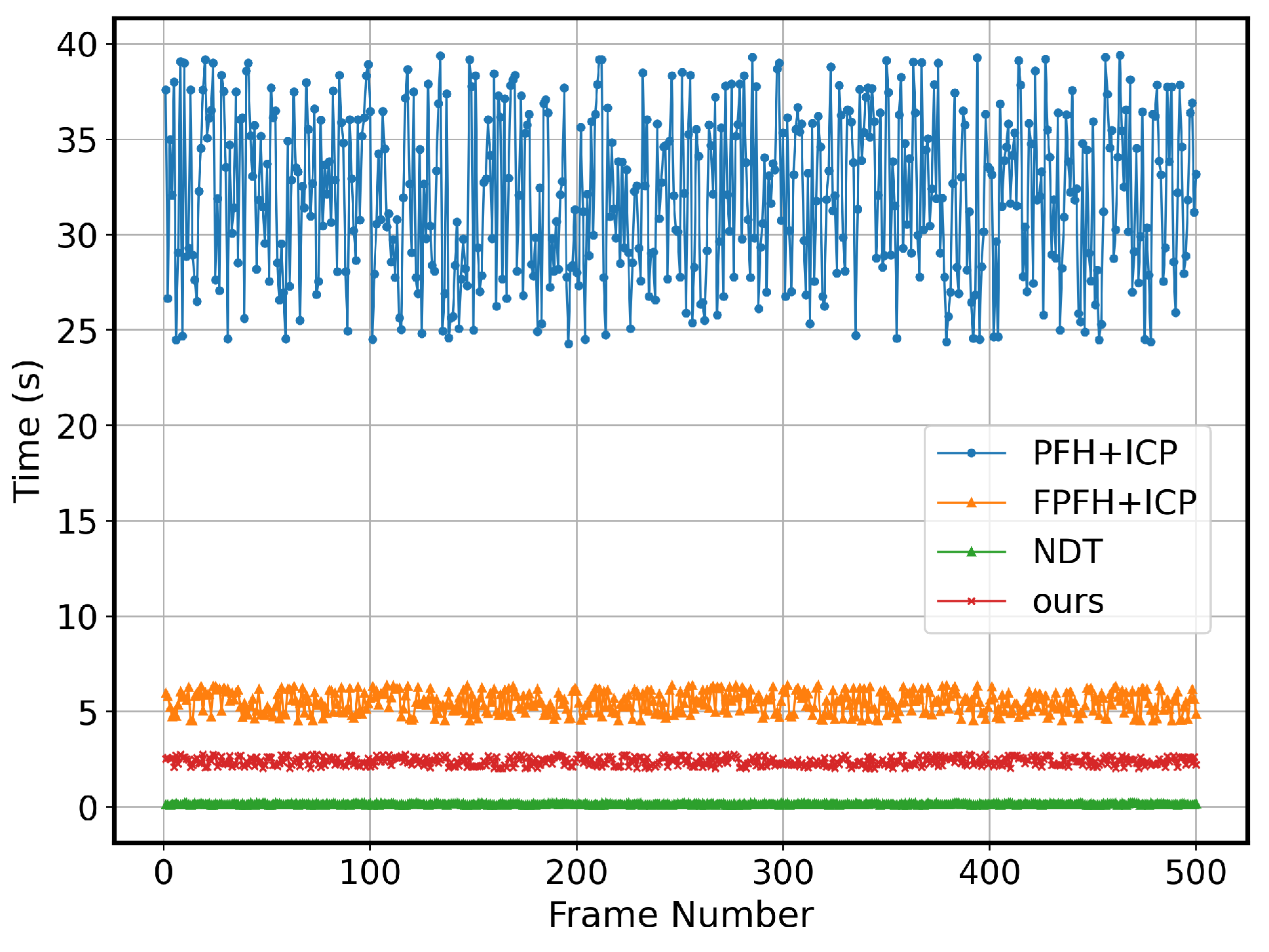
As shown in Figure 7, PFH + ICP [58] and FPFH + ICP [59] exhibit certain limitations in feature description and matching, particularly regarding real-time performance and noise robustness. Although the NDT algorithm [60] performs well in real-time scenarios, its dependence on precise initial values—which are unavailable prior to vehicle calibration—limits its applicability. In contrast, the proposed algorithm does not rely on initial values and achieves efficient registration by utilizing a larger shared observation area, thereby overcoming the limitations inherent in traditional algorithms for practical applications.
Figure 8 shows the running time of 500 consecutive frames: PFH is slowest; FPFH is faster yet still non-real-time; NDT is fastest but initialization-dependent; and ours is close to NDT while initialization-free.
Compared with PFH + ICP, FPFH + ICP, and NDT, our method attains higher extrinsic accuracy by leveraging ground constraints and 2D feature maps with 3D context. Motion consistency filtering reduces noise and computation, enabling robust registration in dynamic scenes.

7.3. Real Vehicle Experiment

The vehicle followed straight and curved paths in a closed area. We precalibrated the integrated navigation module and assumed { V } coincided with { I } .

7.3.1. Calibration Process

We applied the proposed algorithm to each LiDAR in the vehicle. Since the calibration process is identical across sensors, we use the rear LiDAR to illustrate the procedure and results.
  • Ground fitting phase: multi-frame ground RANSAC fitting combined with the Lagrange multiplier method was used to achieve convergence of the ground parameters, as illustrated in Figure 9. The figure shows the initial values of each coefficient during vehicle movement and the changes in optimization results as the number of samples increases. The blue curves represent the initial values of each parameter, while the orange curves show the optimization process. As the vehicle moves, several factors contribute to parameter fluctuations: ground unevenness, suspension vibrations, LiDAR point cloud noise, and errors in ground fitting. After accumulating data over multiple frames, the final plane parameters stabilize, and these parameters are then used for LiDAR ground plane alignment.
  • Initial straight-driving phase: the ground plane was fitted, and the yaw angle γ V L i was estimated using the motion constraint method. During the combined straight and curved driving stages, translation parameters in the X and Y directions were estimated.
  • Optimization of degrees of freedom (DoF) parameters in the dimension-reduced plane: As shown in Figure 10, yaw stabilizes over straight segments, and translation converges over combined segments. Fluctuations reflect registration noise, time synchronization, and sampling effects, and convergence improves with more samples.

7.3.2. Calibration Results and Accuracy Evaluation

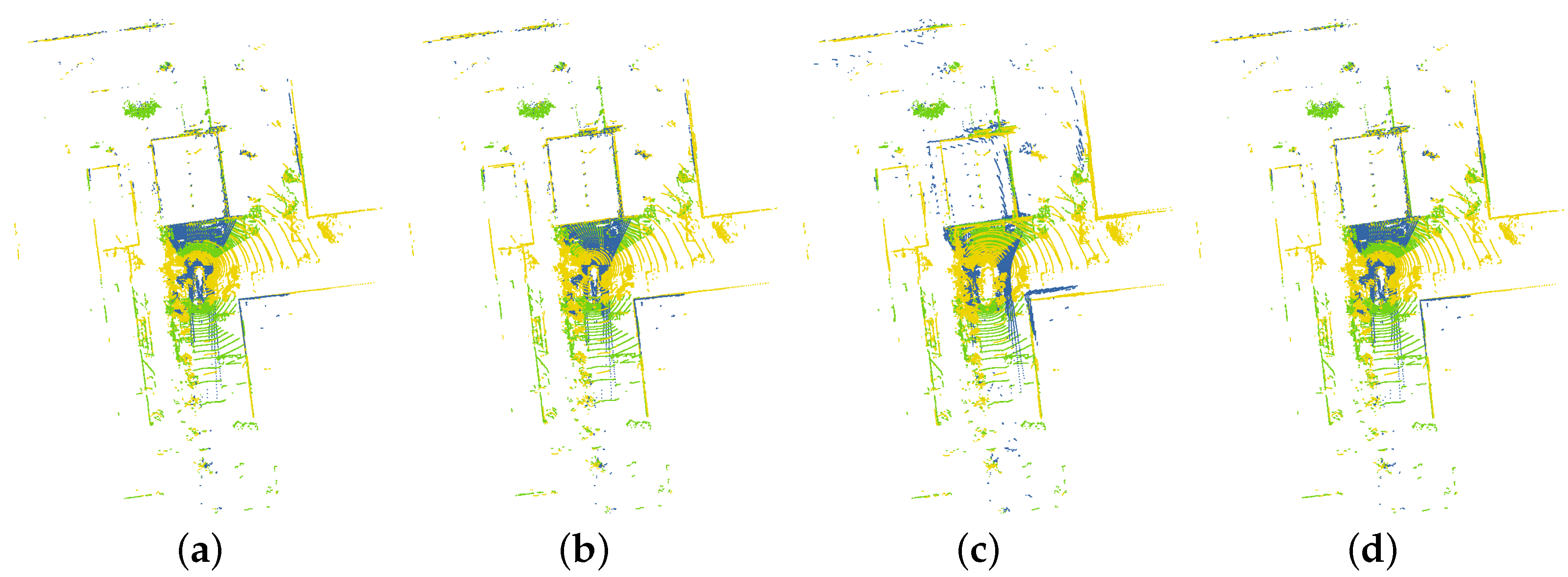
We conducted five trials in a closed test area and report averages. Following OpenCalib [23] and Jiao et al. [24], we obtained baseline calibrations and evaluated accuracy against offline manual calibration (Table 1). All five LiDARs were calibrated and merged into the vehicle frame; Figure 11 shows overlays for OpenCalib [23], Jiao et al. [24], and ours. OpenCalib attains high accuracy with calibration boards but lacks ground-DoF constraints and requires manual intervention. Jiao et al.’s method performs well for near-horizontal layouts but degrades with irregular sensor orientations. Our method is comparable to OpenCalib on average and markedly better than Jiao et al., especially for tilted sensors (e.g., Left/Right Bottom LiDAR), evidencing robustness across configurations. Although slightly higher than offline methods in some cases, errors (max 6.085 cm, 4.768°) meet practical requirements.

7.4. nuScenes Dataset Experiment

We evaluate generalizability on nuScenes using scenes with straight and curved segments, using dataset extrinsics as ground truth to assess cross-platform adaptability.

7.4.1. Calibration Results

Figure 12 shows the convergence of ground fitting parameters in the motion dimensionality reduction stage. Figure 13 shows the yaw angle γ V L and translation vector in the linear and curved compound motion stage. It is worth noting that since the public dataset has a higher precision of multi-sensor time synchronization and positioning accuracy, the convergence speed of each parameter is faster than our real vehicle experiment.
Applying our method to nuScenes (straight and curved trajectories), Figure 12 shows faster convergence of plane parameters; yaw and translation behave similarly due to tighter time synchronization and higher localization accuracy.

7.4.2. Accuracy Evaluation

The calibrated extrinsic parameters were compared with the ground truth provided by the dataset. The maximum translation error was 2.916 cm, and the rotation error was 5.386°. This confirmed the high adaptability of the proposed method to different platforms and demonstrated its efficiency in generating accurate calibration results even under varying sensor configurations.

8. Conclusions

We presented an online multi-LiDAR self-calibration method that reduces motion dimensionality with ground constraints, projects point clouds via a virtual RGB–D camera for efficient registration, and solves hand–eye parameters stepwise with online evaluation. Our key contributions are (i) a virtual RGB–D projection and motion-consistency filtering that enable efficient, target-free, initialization-robust registration; (ii) a stepwise, motion-constrained hand–eye formulation that decouples yaw and translation for stable convergence with limited overlaps and tilted sensors; and (iii) an online evaluator that fuses plane-alignment and multi-odometry to detect drift and trigger recalibration during routine operation. On a commercial vehicle and nuScenes, the method provides accuracy comparable to target-based baselines (max errors 6.058 cm and 4.768° on-vehicle; 2.916 cm and 5.386° on nuScenes) while enabling practical online deployment. Our method assumes near-planar motion and sufficient environmental structure. Performance may degrade on slopes or in feature-sparse scenes. For practical deployment, we recommend using integrated navigation systems to monitor vehicle attitude and ensure operation within acceptable motion constraints. Future work includes adaptive plane handling (e.g., IMU-assisted slope compensation), multimodal cues (camera/radar), and broader evaluation across terrains and weather. The approach is well suited to commercial fleets where sensor poses drift over time. By removing target dependence, operational downtime is reduced.

Author Contributions

Conceptualization, J.H. and Z.Y.; methodology, Y.T. and W.X.; software, Y.T. and S.H.; validation, Y.T., S.H. and B.H.; investigation, Y.T. and J.H.; resources, J.H., Z.Y. and B.H.; data curation, S.H.; writing—original draft, Y.T.; writing—review and editing, Y.T., J.H. and W.X.; visualization, Y.T.; supervision, J.H. and Z.Y.; project administration, Z.Y.; funding acquisition, J.H. and Z.Y. All authors have read and agreed to the published version of the manuscript.

Funding

This research was funded by the Major Program (JD) of Hubei Province (No. 2023BAA017); and the Science and Technology Innovation Talent Program of Hubei Province (No. 2023DJC092).

Institutional Review Board Statement

Not applicable.

Informed Consent Statement

Not applicable.

Data Availability Statement

The data presented in this study are available on request from the corresponding author. The partial dataset supporting the algorithmic findings of this study is publicly available; however, the complete raw dataset is not publicly available due to commercial restrictions.

Acknowledgments

We thank the Commercial Product R&D Institute of Dongfeng Automobile Co., Ltd. for access to the multi-LiDAR vehicle platform and field-testing support, and the nuScenes team for providing the open dataset used in our evaluation. We also thank our colleagues at Wuhan University of Technology and Hubei University of Technology for helpful discussions and feedback.

Conflicts of Interest

Author Bolun Hu was employed by the company Commercial Product R&D Institute, Dongfeng Automobile Co., Ltd. The remaining authors declare that the research was conducted in the absence of any commercial or financial relationships that could be construed as a potential conflict of interest.

References

  1. Huang, J.; Huang, G.; Zhu, Z.; Ye, Y.; Du, D. Bevdet: High-performance multi-camera 3D object detection in bird-eye-view. arXiv 2021, arXiv:2112.11790. [Google Scholar]
  2. Zhou, B.; Krähenbühl, P. Cross-view transformers for real-time map-view semantic segmentation. In Proceedings of the IEEE/CVF Conference Computer Vision and Pattern Recognition, New Orleans, LA, USA, 18–24 June 2022; pp. 13760–13769. [Google Scholar]
  3. Man, Y.; Gui, L.Y.; Wang, Y.X. BEV-guided multi-modality fusion for driving perception. In Proceedings of the IEEE/CVF Conference Computer Vision and Pattern Recognition, Vancouver, BC, Canada, 17–24 June 2023; pp. 21960–21969. [Google Scholar]
  4. Lin, Z.; Liu, Z.; Xia, Z.; Wang, X.; Wang, Y.; Qi, S.; Dong, Y.; Dong, N.; Zhang, L.; Zhu, C. RCBEVDet: Radar-camera fusion in bird’s eye view for 3D object detection. In Proceedings of the IEEE/CVF Conference Computer Vision and Pattern Recognition, Seattle, WA, USA, 16–22 June 2024; pp. 14928–14937. [Google Scholar]
  5. Liang, T.; Xie, H.; Yu, K.; Xia, Z.; Lin, Z.; Wang, Y.; Tang, T.; Wang, B.; Tang, Z. Bevfusion: A simple and robust lidar-camera fusion framework. Adv. Neural Inf. Process. Syst. 2022, 35, 10421–10434. [Google Scholar]
  6. Yang, H.; Zhang, S.; Huang, D.; Wu, X.; Zhu, H.; He, T.; Tang, S.; Zhao, H.; Qiu, Q.; Lin, B.; et al. Unipad: A universal pre-training paradigm for autonomous driving. In Proceedings of the IEEE/CVF Conference Computer Vision and Pattern Recognition, Seattle, WA, USA, 16–22 June 2024; pp. 15238–15250. [Google Scholar]
  7. Chang, D.; Zhang, R.; Huang, S.; Hu, M.; Ding, R.; Qin, X. Versatile Multi-LiDAR Accurate Self-Calibration System Based on Pose Graph Optimization. IEEE Trans. Robot. 2023, 8, 4839–4846. [Google Scholar] [CrossRef]
  8. Fent, F.; Kuttenreich, F.; Ruch, F.; Rizwin, F.; Juergens, S.; Lechermann, L.; Nissler, C.; Perl, A.; Voll, U.; Yan, M.; et al. MAN TruckScenes: A multimodal dataset for autonomous trucking in diverse conditions. arXiv 2024, arXiv:2407.07462. [Google Scholar] [CrossRef]
  9. Gurumadaiah, A.K.; Park, J.; Lee, J.-H.; Kim, J.; Kwon, S. Precise Synchronization Between LiDAR and Multiple Cameras for Autonomous Driving: An Adaptive Approach. IEEE Trans. Intell. Veh. 2025, 10, 2152–2162. [Google Scholar] [CrossRef]
  10. Seidaliyeva, U.; Ilipbayeva, L.; Utebayeva, D.; Smailov, N.; Matson, E.T.; Tashtay, Y.; Turumbetov, M.; Sabibolda, A. LiDAR Technology for UAV Detection: From Fundamentals and Operational Principles to Advanced Detection and Classification Techniques. Sensors 2025, 25, 2757. [Google Scholar] [CrossRef] [PubMed]
  11. Ou, J.; Huang, P.; Zhou, J.; Zhao, Y.; Lin, L. Automatic extrinsic calibration of 3D LIDAR and multi-cameras based on graph optimization. Sensors 2022, 22, 2221. [Google Scholar] [CrossRef]
  12. Zeng, T.; Gu, X.; Yan, F.; He, M.; He, D. YOCO: You Only Calibrate Once for Accurate Extrinsic Parameter in LiDAR-Camera Systems. arXiv 2024, arXiv:2407.18043. [Google Scholar] [CrossRef]
  13. Petek, K.; Vödisch, N.; Meyer, J.; Cattaneo, D.; Valada, A.; Burgard, W. Automatic target-less camera-LiDAR calibration from motion and deep point correspondences. arXiv 2024, arXiv:2404.17298. [Google Scholar] [CrossRef]
  14. Jiao, J.; Yu, Y.; Liao, Q.; Ye, H.; Fan, R.; Liu, M. Automatic calibration of multiple 3D LiDARs in urban environments. In Proceedings of the IEEE/RSJ International Conference Intelligent Robots and Systems, Macau, China, 4–8 November 2019; pp. 15–20. [Google Scholar] [CrossRef]
  15. Wang, F.; Zhao, X.; Gu, H.; Wang, L.; Wang, S.; Han, Y. Multi-Lidar system localization and mapping with online calibration. Appl. Sci. 2023, 13, 10193. [Google Scholar] [CrossRef]
  16. Das, S.; Boberg, B.; Fallon, M.; Chatterjee, S. IMU-based online multi-lidar calibration. In Proceedings of the 2024 IEEE Intelligent Vehicles Symposium, Jeju Island, Republic of Korea, 2–5 June 2024; pp. 3227–3234. [Google Scholar]
  17. Gao, C.; Spletzer, J.R. On-line calibration of multiple LIDARs on a mobile vehicle platform. In Proceedings of the IEEE International Conference Robotics and Automation, Anchorage, AK, USA, 3–8 May 2010; pp. 279–284. [Google Scholar] [CrossRef]
  18. Yoo, J.H.; Jung, G.B.; Jung, H.G.; Suhr, J.K. Camera-LiDAR calibration using iterative random sampling and intersection line-based quality evaluation. Electronics 2024, 13, 249. [Google Scholar] [CrossRef]
  19. Liu, Y.; Cui, X.; Fan, S.; Wang, Q.; Liu, Y.; Sun, Y.; Wang, G. Dynamic validation of calibration accuracy and structural robustness of a multi-sensor mobile robot. Sensors 2024, 24, 3896. [Google Scholar] [CrossRef]
  20. Lee, H.; Chung, W. Extrinsic calibration of multiple 3D LiDAR sensors by the use of planar objects. Sensors 2022, 22, 7234. [Google Scholar] [CrossRef]
  21. Choi, D.G.; Bok, Y.; Kim, J.S.; Kweon, I.S. Extrinsic calibration of 2-D lidars using two orthogonal planes. IEEE Trans. Robot. 2015, 32, 83–98. [Google Scholar] [CrossRef]
  22. Shi, B.; Yu, P.; Yang, M.; Wang, C.; Bai, Y.; Yang, F. Extrinsic calibration of dual LiDARs based on plane features and uncertainty analysis. IEEE Sens. J. 2021, 21, 11117–11130. [Google Scholar] [CrossRef]
  23. Yan, G.; Liu, Z.; Wang, C.; Shi, C.; Wei, P.; Cai, X.; Ma, T.; Liu, Z.; Zhong, Z.; Liu, Y.; et al. Opencalib: A multi-sensor calibration toolbox for autonomous driving. Softw. Impacts 2022, 14, 100393. [Google Scholar] [CrossRef]
  24. Jiao, J.; Liao, Q.; Zhu, Y.; Liu, T.; Yu, Y.; Fan, R. A novel dual-lidar calibration algorithm using planar surfaces. In Proceedings of the 2019 IEEE Intelligent Vehicles Symposium, Paris, France, 9–12 June 2019; pp. 1499–1504. [Google Scholar]
  25. Nie, M.; Shi, W.; Fan, W.; Xiang, H. Automatic extrinsic calibration of dual LiDARs with adaptive surface normal estimation. IEEE Trans. Instrum. Meas. 2022, 72, 1000711. [Google Scholar] [CrossRef]
  26. Claussmann, L.; Revilloud, M.; Gruyer, D.; Glaser, S. A review of motion planning for highway autonomous driving. IEEE Trans. Intell. Transp. Syst. 2019, 21, 1826–1848. [Google Scholar] [CrossRef]
  27. Teng, S.; Hu, X.; Deng, P.; Li, B.; Li, Y.; Ai, Y. Motion planning for autonomous driving: The state of the art and future perspectives. IEEE Trans. Intell. Veh. 2023, 8, 3692–3711. [Google Scholar] [CrossRef]
  28. Kong, J.; Pfeiffer, M.; Schildbach, G.; Borrelli, F. Kinematic and dynamic vehicle models for autonomous driving control design. In Proceedings of the 2015 IEEE Intelligent Vehicles Symposium, Seoul, Republic of Korea, 28 June–1 July 2015; pp. 1094–1099. [Google Scholar]
  29. Chen, L.; Wu, P.; Chitta, K.; Jaeger, B.; Geiger, A.; Li, H. End-to-end autonomous driving: Challenges and frontiers. IEEE Trans. Pattern Anal. Mach. Intell. 2024, 46, 10164–10183. [Google Scholar] [CrossRef]
  30. Jiao, J.; Ye, H.; Zhu, Y.; Liu, M. Robust Odometry and Mapping for Multi-LiDAR Systems With Online Extrinsic Calibration. IEEE Trans. Robot. 2022, 2022, 351–371. [Google Scholar] [CrossRef]
  31. Huang, G.; Huang, H.; Xiao, W.; Dang, Y.; Xie, J.; Gao, X.; Huang, Y. A sensor fusion-based optimization method for indoor localization. In Proceedings of the Fourth International Conference Mechanical Engineering, Intelligent Manufacturing, and Automation Technology (MEMAT 2023), Guilin, China, 20–22 October 2023; Volume 13082, pp. 184–190. [Google Scholar]
  32. Liu, X.; Zhang, F. Extrinsic calibration of multiple LiDARs of small FoV in targetless environments. IEEE Robot. Autom. Lett. 2021, 6, 2036–2043. [Google Scholar] [CrossRef]
  33. Kim, T.Y.; Pak, G.; Kim, E. GRIL-Calib: Targetless Ground Robot IMU-LiDAR extrinsic calibration method using ground plane motion constraints. IEEE Robot. Autom. Lett. 2024, 9, 5409–5416. [Google Scholar] [CrossRef]
  34. Della Corte, B.; Andreasson, H.; Stoyanov, T.; Grisetti, G. Unified motion-based calibration of mobile multi-sensor platforms with time delay estimation. IEEE Robot. Autom. Lett. 2019, 4, 902–909. [Google Scholar] [CrossRef]
  35. Yin, J.; Yan, F.; Liu, Y.; Zhuang, Y. Automatic and targetless LiDAR-Camera extrinsic calibration using edge alignment. IEEE Sens. J. 2023, 23, 19871–19880. [Google Scholar] [CrossRef]
  36. Yu, J.; Vishwanathan, S.V.N.; Günter, S.; Schraudolph, N.N. A quasi-Newton approach to non-smooth convex optimization. In Proceedings of the 25th International Conference Machine Learning, Helsinki, Finland, 5–9 July 2008. [Google Scholar]
  37. Caponetto, R.; Fortuna, L.; Graziani, S.; Xibilia, M.G. Genetic algorithms and applications in system engineering: A survey. Trans. Inst. Meas. Control 1993, 15, 143–156. [Google Scholar] [CrossRef]
  38. Tan, Z.; Zhang, X.; Teng, S.; Wang, L.; Gao, F. A Review of Deep Learning-Based LiDAR and Camera Extrinsic Calibration. Sensors 2024, 24, 3878. [Google Scholar] [CrossRef]
  39. Liao, Y.; Li, J.; Kang, S. SE-Calib: Semantic edges based LiDAR-camera boresight online calibration in urban scenes. IEEE Trans. Geosci. Remote Sens. 2023, 61, 1000513. [Google Scholar] [CrossRef]
  40. Liu, Z.; Tang, H.; Zhu, S.; Han, S. SemAlign: Annotation-free camera-LiDAR calibration with semantic alignment loss. In Proceedings of the 2021 IEEE/RSJ International Conference Intelligent Robots and Systems, Prague, Czech Republic, 27 September–1 October 2021; pp. 15–20. [Google Scholar] [CrossRef]
  41. Zhu, J.; Xue, J.; Zhang, P. CalibDepth: Unifying depth map representation for iterative LiDAR-camera online calibration. In Proceedings of the 2023 IEEE International Conference Robotics and Automation, London, UK, 29 May–2 June 2023; pp. 279–284. [Google Scholar] [CrossRef]
  42. Wu, X.; Zhang, C.; Liu, Y. CalibRank: Effective LiDAR-camera extrinsic calibration by multi-modal learning to rank. In Proceedings of the IEEE International Conference Image Processing, Abu Dhabi, United Arab Emirates, 27–30 October 2020; pp. 2152–2162. [Google Scholar] [CrossRef]
  43. Iyer, G.; Murthy, J.K.; Krishna, K.M. CalibNet: Self-supervised extrinsic calibration using 3D spatial transformer networks. In Proceedings of the 2018 IEEE/RSJ International Conference Intelligent Robots and Systems, Madrid, Spain, 1–5 October 2018; pp. 1–5. [Google Scholar] [CrossRef]
  44. Yuan, K.; Guo, Z.; Wang, Z.J. RGGNet: Tolerance aware LiDAR-camera online calibration with geometric deep learning and generative model. IEEE Robot. Autom. Lett. 2020, 5, 6956–6963. [Google Scholar] [CrossRef]
  45. Lv, X.; Wang, B.; Dou, Z.; Ye, D.; Wang, S. LCCNet: LiDAR and camera self-calibration using cost volume network. In Proceedings of the 2021 IEEE/CVF Conference Computer Vision and Pattern Recognition Workshops, Nashville, TN, USA, 19–25 June 2021; pp. 20–25. [Google Scholar] [CrossRef]
  46. Mharolkar, S.; Zhang, J.; Peng, G.; Liu, Y.; Wang, D. RGBDTCalibNet: End-to-end online extrinsic calibration between a 3D LiDAR, an RGB camera and a thermal camera. In Proceedings of the IEEE 25th International Conference Intelligent Transportation Systems, Macau, China, 8–12 October 2022; pp. 8–12. [Google Scholar] [CrossRef]
  47. Yu, Z.; Feng, C.; Liu, M.Y.; Ramalingam, S. CaseNet: Deep category-aware semantic edge detection. In Proceedings of the 2017 IEEE Conference Computer Vision and Pattern Recognition, Honolulu, HI, USA, 21–26 July 2017; pp. 21–26. [Google Scholar] [CrossRef]
  48. Kang, J.; Doh, N.L. Automatic targetless camera-lidar calibration by aligning edge with gaussian mixture model. J. Field Robot. 2020, 37, 158–179. [Google Scholar] [CrossRef]
  49. Tao, L.; Pei, L.; Li, T.; Zou, D.; Wu, Q.; Xia, S. CPI: LiDAR-camera extrinsic calibration based on feature points with reflection intensity. In Proceedings of the Spatial Data and Intelligence 2020, Shenzhen, China, 8–9 May 2020; pp. 8–9. [Google Scholar] [CrossRef]
  50. Wang, W.; Nobuhara, S.; Nakamura, R.; Sakurada, K. SOIC: Semantic online initialization and calibration for LiDAR and camera. arXiv 2020, arXiv:2003.04260. [Google Scholar] [CrossRef]
  51. Derpanis, K.G. Overview of the RANSAC algorithm. Image Rochester NY 2010, 4, 2–3. [Google Scholar]
  52. Bertsekas, D.P. Constrained Optimization and Lagrange Multiplier Methods; Academic Press: Cambridge, MA, USA, 2014. [Google Scholar]
  53. Dai, J.S. Euler–Rodrigues formula variations, quaternion conjugation and intrinsic connections. Mech. Mach. Theory 2015, 92, 144–152. [Google Scholar] [CrossRef]
  54. Rublee, E.; Rabaud, V.; Konolige, K.; Bradski, G. ORB: An efficient alternative to SIFT or SURF. In Proceedings of the 2011 International Conference Computer Vision, Barcelona, Spain, 6–13 November 2011; pp. 2564–2571. [Google Scholar]
  55. Calonder, M.; Lepetit, V.; Strecha, C.; Fua, P. Brief: Binary robust independent elementary features. In Proceedings of the Computer Vision–ECCV 2010, Heraklion, Crete, Greece, 5–11 September 2010; pp. 778–792. [Google Scholar]
  56. Rusinkiewicz, S.; Levoy, M. Efficient variants of the ICP algorithm. In Proceedings of the 3rd International Conference 3-D Digital Imaging and Modeling, Quebec City, QC, Canada, 28 May–1 June 2001. [Google Scholar]
  57. Hsieh, C.-C. B-spline wavelet-based motion smoothing. Comput. Ind. Eng. 2001, 41, 59–76. [Google Scholar] [CrossRef]
  58. Rusu, R.B.; Blodow, N.; Marton, Z.C.; Beetz, M. Aligning point cloud views using persistent feature histograms. In Proceedings of the IEEE/RSJ International Conference Intelligent Robots and Systems, Nice, France, 22–26 September 2008. [Google Scholar]
  59. Rusu, R.B.; Blodow, N.; Beetz, M. Fast point feature histograms (FPFH) for 3D registration. In Proceedings of the IEEE International Conference Robotics and Automation, Kobe, Japan, 12–17 May 2009. [Google Scholar]
  60. Biber, P.; Straßer, W. The normal distributions transform: A new approach to laser scan matching. In Proceedings of the IEEE/RSJ International Conference Intelligent Robots and Systems (IROS), Las Vegas, NV, USA, 27–31 October 2003; Volume 3. [Google Scholar]
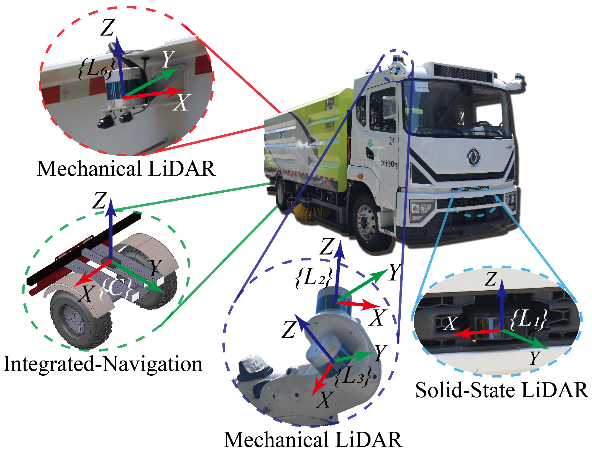
Figure 1. Commercial vehicle platform: one 128-line solid-state primary LiDAR and five 32-line mechanical LiDARs; positioning via a high-precision integrated navigation module (IMU/GNSS/RTK).
Mathematics 13 03181 g001
Figure 2. Overview. Phase 1 (Preprocessing): ground plane alignment reduces motion DoF, and a virtual RGB–D projection yields 2D feature/depth maps with ORB/ICP registration. Phase 2 (Optimization for Hand–Eye Calibration): stepwise estimation—yaw from straight segments, translation from curved/compound motion. Phase 3 (Error Evaluation): plane alignment and LiDAR–INS odometry consistency checks trigger recalibration.
Mathematics 13 03181 g002
Figure 3. Comparison of LiDAR point clouds before and after ground alignment. (a) Original point cloud: The ground points, shown in red, lie predominantly below the X O Y plane, indicating a misalignment. (b) Aligned point cloud: After processing with our algorithm, the ground points (now green) are aligned with the X O Y plane and above it. This allows the vehicle to be treated as moving on the X O Y plane, effectively reducing the dimensionality of its motion.
Mathematics 13 03181 g003
Figure 4. Principle of virtual camera imaging. A virtual RGB–D camera positioned above the point cloud captures the complete point cloud after removing ground points. This process generates an RGB feature map with intensity characteristics and a depth map with depth values.
Mathematics 13 03181 g004
Figure 5. Feature maps under different camera parameters: (a) A relatively small FOV of 30°, resulting in a feature map with minimal distortion. (b) A relatively large FOV of 120°, resulting in a feature map with significant distortion, but capturing more spatial details.
Mathematics 13 03181 g005
Figure 6. Feature matching and motion consistency filtering: (a) Original ORB matching results without filtering incorrect matching pairs. (b) Results after filtering incorrect matches using the motion consistency principle. The green and red borders indicate the current and previous frames, respectively.
Mathematics 13 03181 g006
Figure 7. A comparison of registration methods on consecutive point cloud frames (blue and green, respectively): (a) PFH: strong descriptors but noise-sensitive. (b) FPFH: faster yet still noise-sensitive. (c) NDT: fast but requires good initialization. (d) Ours: robust results without strong initialization in planar motion.
Mathematics 13 03181 g007
Figure 8. Computation time across registration methods. NDT is fastest but requires good initialization; PFH/FPFH are slower. Our method is slightly slower than NDT yet initialization-free and practical for real-time use.
Mathematics 13 03181 g008
Figure 9. Convergence of ground fitting equation coefficients during motion dimensionality reduction. The parameters are the coefficients of the plane fitting equation a x + b y + c z + d = 0 . (a) The x-component of the plane’s normal vector. (b) The y-component of the plane’s normal vector. (c) The z-component of the plane’s normal vector. (d) The distance parameter, related to the signed distance from the origin.
Mathematics 13 03181 g009
Figure 10. Optimization of DoF in the dimension-reduced plane. White: straight segments (yaw optimization); gray: curved segments (translation optimization). Translation may exhibit local minima before convergence.
Mathematics 13 03181 g010
Figure 11. Merged multi-LiDAR point clouds (Each color represents the data from a distinct LiDAR viewpoint): (a) Manual (baseline). (b) OpenCalib [23]: limited ground alignment. (c) Jiao et al. [24]: degraded for tilted LiDARs. (d) Proposed: consistent overlap and ground alignment across sensors.
Mathematics 13 03181 g011
Figure 12. Convergence of plane coefficients for nuScenes during motion dimensionality reduction. The parameters are the coefficients of the plane fitting equation a x + b y + c z + d = 0 . (a) The x-component of the plane’s normal vector. (b) The y-component of the plane’s normal vector. (c) The z-component of the plane’s normal vector. (d) The distance parameter, related to the signed distance from the origin.
Mathematics 13 03181 g012
Figure 13. Optimization of planar DoF on nuScenes: straight (white) for yaw; curved/compound (gray) for translation. Faster convergence benefits from tighter synchronization and localization.
Mathematics 13 03181 g013
Table 1. Calibration errors of the proposed method versus benchmark methods.
LiDAR NameOpenCalib [23]Jiao et al. [23]Ours
Translation
Error (cm)
Rotation
Error (°)
Translation
Error (cm)
Rotation
Error (°)
Translation
Error (cm)
Rotation
Error (°)
Primary2.6582.1265.1523.2525.2763.158
Rear3.6911.2968.7016.1546.0854.768
Left Top2.5213.0962.7113.0885.3122.186
Left Bottom3.1543.64263.15745.6426.0232.956
Right Top3.7342.5017.6067.6425.6243.246
Right Bottom4.5991.577126.15430.6543.6814.036
Disclaimer/Publisher’s Note: The statements, opinions and data contained in all publications are solely those of the individual author(s) and contributor(s) and not of MDPI and/or the editor(s). MDPI and/or the editor(s) disclaim responsibility for any injury to people or property resulting from any ideas, methods, instructions or products referred to in the content.