Abstract
The article presents a new method for multi-agent traffic flow balancing. It is based on the MAROH multi-agent optimization method. However, unlike MAROH, the agent’s control plane is built on the principles of human decision-making and consists of two layers. The first layer ensures autonomous decision-making by the agent based on accumulated experience—representatives of states the agent has encountered and knows which actions to take in them. The second layer enables the agent to make decisions for unfamiliar states. A state is considered familiar to the agent if it is close, in terms of a specific metric, to a state the agent has already encountered. The article explores variants of state proximity metrics and various ways to organize the agent’s memory. It has been experimentally shown that an agent with the proposed two-layer control plane SAMAROH-2L outperforms the efficiency of an agent with a single-layer control plane, e.g., makes decisions faster, and inter-agent communication reduction varies from 1% to 80% depending on the selected similarity threshold comparing the method with simultaneous actions SAMAROH and from 80% to 96% comparing to MAROH.
MSC:
68T42; 68M10
1. Introduction
The growth of the size of data communication networks and increasing channel capacity require continuous improvements in methods for balancing data flows in the network. The random nature of the load and its high volatility make classical optimization methods inapplicable [1]. Multicommodity Flow methods, which belong to the class of NP-complete problems, also fail to address the issue, making their use inefficient for data flow balancing [2,3,4]. Consequently, significant attention has been paid to researching the applicability of machine learning methods for balancing.
The paper [5] presented the Multi-Agent Routing using Hashing (MAROH) balancing method based on a combination of the following techniques: multi-agent optimization, reinforcement learning (RL), and consistent hashing (this method is described in detail in Section 3). Experiments showed that MAROH outperformed popular methods like the Equal-cost Multi-Path (ECMP) and Unequal-cost Multi-Path (UCMP) in terms of efficiency.
This method involved the mutual exchange of data about agent states, which burdened the network’s bandwidth. The more agents involved in the exchange process, the greater this burden became. The construction of a new agent state and its action also required certain computations. Besides this, MAROH was based on a sequential decision-making model: only one agent, selected in a specific way, could change the flow distribution. Such organization assumes that the entire exchange process will be repeated multiple times for flow distribution adjustments.
The new method presented in this article aimed to reduce the number of inter-agent communications and the time for an agent to make an optimal action, as well as to remove the sequential agent activation model, thereby accelerating balancing and reducing the network load.
The number of inter-agent communications was reduced by the following. Agents could act independently of each other after exchanging information with neighbors, thereby constraining the number of inter-agent communications as the time of a balancing process. The second novelty is the approach inspired by Nobel winner Daniel Kahneman’s research on human decision-making under uncertainty [6]. The common point of human decision-making and network agent decision-making is that they operate in a situation of uncertainty. Therefore, by analogy with the two-system model of human decision-making proposed in [6] (fast intuitive and slow analytical reactions), the agent’s control plane was divided into two layers: experience and decision-making. The experience layer is activated when the current state is familiar to the agent, i.e., it is close, in terms of the metric, to a state the agent has encountered before. In this case, the agent applies the action that was previously successful without any communication with other agents. If the current state is unfamiliar, i.e., it is farther than a certain threshold from all familiar states, the agent activates the second layer responsible for the processing of an unfamiliar state, decision-making, and experience updating. It is important to note that this is a loose conceptual analogy rather than a strict implementation.
Thus, the main contributions of the article are the ways to reduce the number of inter-agent interactions, as well as the time and computational costs for agent decision-making, by
- Replacing the sequential activation scheme of agents with the new scheme of independent agent activation (experiments showed this achieves a flow distribution close to optimal);
- Inventing algorithms for a two-layer agent control plane that allows one to reduce the number of inter-agent exchanges and accelerates agent decision-making.
The rest of the article is the following. Section 2 reviews works that use the agent-states history. Section 3 describes the MAROH method [5] that was used as the basis for the proposed new method. Section 4 presents proposed novelty solutions. Section 5 describes an experimental methodology. The experimental results are presented in Section 6, and Section 7 discusses the achievements.
2. Related Work
Recent advances in multi-agent reinforcement learning have focused on improving coordination while mitigating communication overhead. Among these, Communication-Enhanced Value Decomposition Multi-Agent Reinforcement Learning (CVDMARL) [7] reduces the communication overhead by integrating a gated recurrent unit (GRU) to mine the temporal features in the historical data and obtain the communication matrix. In contrast to such methods that still rely on communication, albeit reduced, our proposed method eliminates the need for inter-agent messaging entirely in familiar states.
BayesIntuit [8] introduces the Dynamic Memory Bank—given a query, it retrieves a memory from the same semantic cluster, approximating nearest-neighbor retrieval in the learned latent space. Cosine similarity between the retrieved memory and current representation is used to provide a reliability score. However, BayesIntuit is developed for a single-agent supervised learning algorithm.
An analysis of publications revealed only a few papers [9,10,11] that consider a two-layer approach in combination with reinforcement learning. The work [9] provides an overview of memory-based methods, but they are focused on single-agent reinforcement learning. The study [10] proposes an approach based on episodic memory in a multi-agent setting, but the memory is used in a centralized manner to improve the training process. The work [11] outlines preliminary ideas with the lack of a detailed description of the proposed two-layer approach and presents only a simplified experimental study.
Memory Augmented Multi-Agent Reinforcement Learning for Cooperative Environments [12] incorporates long-short-term memory (LTSM) into actors and critics to enhance MARL performance. This augmentation facilitates the extraction of relevant information from history, which is then combined with the extracted features from the current observations. However, this method is not designed to reduce inter-agent exchanges.
In [13], the asynchronous operating of agents is considered to balance data flows between servers in data centers, but no interaction between agents is assumed. In [14], a case is considered where agents can act simultaneously, but the number of agents acting in parallel is limited by a constant.
3. Background
As mentioned earlier, the developed method is based on MAROH. Here, a brief description of MAROH is provided, necessary for understanding the new method. In MAROH, each agent manages one channel and calculates the weight of its channel to achieve uniform channel loading (see Figure 1). Uniformity is ensured by the multi-agent optimization of the functional Φ, which is the value of the channel load deviation from the average network load:
where is the occupied channel bandwidth, is the nominal channel bandwidth, and
is the average channel load in the network.
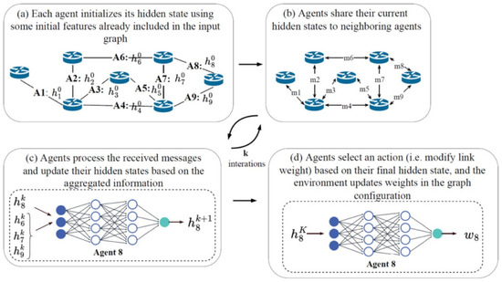
Figure 1.
Schematic of the MAROH method [5].
The choice of functional Φ directly corresponds to the core optimization target of our method—balancing channel utilization—and aligns with the metrics used in prior works (e.g., MAROH, ECMP) for fair comparison. Balanced load distribution lowers congestion that leads to lower delays and packet loss, important for traffic engineering methods. However, our main contribution is communication-efficient learning architecture, so we did not conduct experiments with distinct quality metrics.
Balancing consists of distributing data flows proportionally to channel weights. This way makes the agent operation independent of the number of channels on a network device. The agent state is a pair of channel weights and channel loads (Figure 1a). Each agent, upon changing its state (called a hidden state), transmits its state to the agent neighbors (Figure 1b). Neighbors are agents on adjacent nodes in the network topology. Each agent processes the received hidden states from neighbors using a graph neural network, which is the Message Passing Neural Network (MPNN). The collected hidden states are processed by the agent’s special neural network, referred to as the “update,” which calculates the agent’s new hidden state (Figure 1c). This process is repeated K times. The value of K determines the size of the agent neighborhood domain, i.e., how many states of other agents are involved in the calculation of the current hidden state. K is a method parameter. After K iterations, the resulting hidden state is fed into a special neural network, referred to as the “readout”. Outputs of the readout network are used to select an action for weight adjustment by the softmax function. In Figure 1d, the readout neural network operation finishing with a new weight is shown. The steps of action selection are omitted there. Possible actions for weight calculation include the following:
- Addition: +1;
- Null action: +0;
- Multiplication: ×k (k is a tunable parameter);
- Division: /k (k is a tunable parameter).
MAROH agents update weights not upon the arrival of each new flow but only when the channel load changing exceeds a specified threshold. In this way, feedback on channel load fluctuations is regulated, which minimizes the overhead of the agent’s operation. New flows are distributed according to the current set of weights without delay for the agent’s decisions. However, outdated weights may lead to suboptimal channel loading, so it is crucial for agents in the proposed method to decide on weight adjustments as quickly as possible.
The network load-balancing problem addressed by the MAROH method is formalized as a Decentralized Partially Observable Markov Decision Process (Dec-POMDP), defined by the tuple , where
- is the global state of the entire network. This includes the weight and load of every channel in the network. This full state is not accessible to any single agent.
- is the joint action space, defined as the Cartesian product of each agent’s action space: As mentioned previously, the action space for each agent consists of weight modification actions.
- is the state transition probability function. This function is complex and unknown, sampled from the real network or a simulation.
- is the global reward and is defined as the difference in values of the objective function (1).
- is the set of joint observations. Each agent n receives a private observation containing the weight and load of its assigned channel.
- is the deterministic observation function that maps the state s and action a to a joint observation o.
- Γ is the discount factor , which determines how much an agent values future rewards compared to immediate ones.
4. Proposed Methods
This section presents solutions that allow agents to operate independently and transform the agent control plane into a two-layer one.
4.1. Simultaneous Actions MAROH (SAMAROH)
Let us introduce some terms. The time interval between agent hidden state initialization and action selection is called a horizon. For an agent, a new horizon begins when the channel load changes beyond a specified threshold. An episode is a fixed number of horizons required for the agent to establish the optimal channel weight. The limitation (only one agent acting) in MAROH was introduced for the theoretical justification of its convergence. However, experiments showed that convergence to the optimal solution persists even with asynchronous agent actions.
Let us consider the number of horizons required to achieve optimal weights by MAROH and by simultaneously acting agents. Let { is the set of optimal weights. For simplicity, suppose the agents are allowed perform an action to only add one to the weight (consideration with other actions is similar). In this case, MAROH will take actions (and thus horizons) to achieve optimal weights. When agents operate independently, they only need horizons. Therefore, independent agents operating can significantly reduce the time to obtain the optimal weights and reduce the number of horizons. For example, for a rhombus topology with eight agents, about 100 horizons are needed, but 20 is enough in the case of an independent agent operating.
In our experimental research, we implemented an abstraction where the algorithm progressed through a sequence of discrete horizons. The length of an episode (i.e., the number of horizons it contains) was treated as a hyperparameter whose optimal value was discovered empirically and shown in Section 5.
In the new approach called SAMAROH (Simultaneous Actions MAROH), all agents can independently adjust weights in each of their horizons. To simplify convergence, following [14], the number of agent actions was reduced to
- Multiplication: ×k (k is a tunable parameter);
- Null action: +0.
Algorithm 1 outlines the pseudo-code for agent decision-making under simultaneous action execution. The key modification compared to MAROH is implemented in lines 11–13, where each agent now computes its local policy and independently selects an action.
| Algorithm 1. SAMAROH operation | |
| 1: | Agents initialize their states based on link bandwidth and initial weight |
| 2: | for t ← 0 to T do |
| 3: | ← (,0,…,0) |
| 4: | for k ← 0 to K do |
| 5: | Agents share their current hidden state to neighboring agents B(v) |
| 6: | Agents process the received messages: ← |
| 7: | Agents update their hidden state ← |
| 8: | end for |
| 9: | Agents compute their actions’ logits: ← |
| 10: | Agents compute the local policy ← CategoricalDist() |
| 11: | Agents select an action according to policy |
| 12: | All agents execute its corresponding action |
| 13: | Agents update their states |
| 14: | Evaluation of Φ |
| 15: | end for |
In MAROH, agents at each horizon selected a single agent and the action it would perform. This occurred as follows: each agent collected a vector of readout neural network outputs from all other agents and applied the softmax function to select the best action. In SAMAROH, the agent collects only a local vector with the readout output for each action, further reducing inter-agent exchanges. Unlike [14], where the number of acting agents was restricted by a constant, our approach allows all agents to act independently. Experimental results (see Section 6) show that this does not affect the method’s accuracy.
4.2. Two-Layer Control Plane MAROH (MAROH-2L)
The second innovation, based on [6], divides the control plane into two layers: experience and decision-making, detailed below.
4.2.1. Experience Layer
Each agent stores past hidden states and corresponding actions. Their collection is called the agent’s memory. Denote the memory of the -th agent as :
where is the hidden state of agent before the (+1)-th exchange iteration, is the memory size (number of stored states), is the number of agents in the system, is the maximum number of exchange iterations, and is the action taken by the agent after completing exchange iterations.
When assessing how close the current state is to familiar states, the agent takes into account all the past hidden states at all intermediate iterations of the exchange in MPNN . This allows familiar states to be identified during the progression toward the horizon.
The second component of a memory element is the agent action, taken after the final -th exchange iteration. However, it is possible to store the input or output of the readout network and reconstruct the selected action. In this case, an ε-greedy strategy can be applied to the agent’s decision-making process to improve learning efficiency [15], and the readout network can be further trained.
Let us call a case a possible memory element. Denote as the set of all cases, i.e., possible memory elements that may arise for an agent. Let Δ: , called the threshold. Denote as the metric on , where . Recall that is symmetric, non-negative, and satisfies the triangle inequality. If , and are called close. A case is familiar to the i-th agent if .
Hidden states are vectors resulting from neural network transformations. The components of vector are numerical representations obtained through nonlinear neural network transformations without direct interpretable meaning. The dimensionality of the hidden state does not have significant importance. It directly affects the volume of messages exchanged between agents, as each message size linearly depends on . Moreover, the choice of a value of allows for balancing the trade-off between the objective function’s value and network load. As it was shown in [5], increasing generally improves the balancing quality but increases the overhead.
To measure the distance between vectors on the experience layer, the following two metrics were used:
- Euclidean metric (L2):
- Manhattan metric (L1):
These metrics were chosen due to the equal significance of hidden state vector components and low computational complexity. Their comparative analysis is detailed in Section 6. In addition to the aforementioned metrics, the cosine distance (Cos) was also applied to measure the distance between vectors on the experience layer:
The cosine distance is not formally a metric, as it does not satisfy the triangle inequality. Nevertheless, as shown in [16], the problem of determining a cosine similarity neighborhood can be transformed into the problem of determining the Euclidean distance, and the cosine distance is widely used in machine learning [8,17].
Since the agent’s memory size is limited, it only includes hidden states called representatives. The choice of representatives is discussed in Section 4.2.2 and Section 4.2.3. Although is considered as prefixed in this paper, the two-layer method could be generalized to the case that is specific for each representative. The value of is the parameter balancing the trade-off between the number of transmitted messages (i.e., how many close states are detected) and the solution quality. Each metric requires individual threshold tuning. The schematic of experience layer is shown in Figure 2.
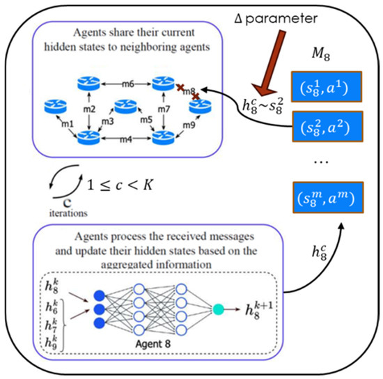
Figure 2.
Schematic of the experience layer operation for the eighth agent.
Depending on the method for selecting representatives for hidden states, there may be alternatives when, for the same hidden state, there is either a single representative (Section 4.2.3) or there are multiple representatives (Section 4.2.2). In the latter, the agent selects the representative with the minimal distance .
There may be cases where the agent memory stores suboptimal actions, as agents are not fully trained or employ an ε-greedy strategy [15]. Therefore, in the two-layer method, when a representative is found, an additional parameter is used to determine the probability of transition to the experience layer. That is, with a certain probability, the agent may start interacting with other agents to improve its action selection, even if a representative for the current state exists in memory.
4.2.2. Decision-Making Layer
At the decision-making layer, the agent, by communicating with other agents, selects an action for a new, unfamiliar state, as in MAROH. At this layer, the agent enriches its memory by adding a new representative. Recall that the agent’s memory does not store all familiar cases but their representatives. There were two ways explored to determine the representatives: experimentally, based on clustering methods, and theoretically, based on constructing an -net [18] (an -net is a subset of a metric space for such that that is no farther than ε from x. Since we are working in a metric space and the set of agent states is finite, an -net exists for it). Let be the threshold—which will also serve as for the -net—the metric value beyond which a state is considered unfamiliar.
Consider the process of selecting memory representatives based on clustering. It is clear that clustering is computationally more complex than the -net way and does not guarantee a single representative for a state.
Initially, when the memory is empty, all hidden states are stored until the memory is exhausted. The hidden states are added to the memory upon the MPNN message processing cycle completing and actions are known.
Any state without a representative in memory is a new candidate for representation. To avoid heavy clustering for each new candidate, they are gathered in a special array . Once this array is full, the joint clustering of arrays and into clusters is performed. After clustering, candidates and existing representatives are merged into clusters by metric , leaving one random state per cluster as the memory representative. Thus, after clustering, selected states remain in , and is cleared. Several clustering algorithms can be used to find representatives. In [11], Mini-Batch K-Means showed the best performance in terms of complexity and message volume. However, since this algorithm only works with (4), Agglomerative Clustering [19] was used for other metrics.
Algorithm 2 outlines the pseudo-code for agent decision-making with two-layer control planes. The experience layer is implemented in lines 5–7, whereas the decision-making layer comprises the remaining lines. Additional logic for experience updates is introduced in lines 8 and 17. The proposed clustering approach is encapsulated within line 8. Line 17 is required since the action is undefined at line 8.
| Algorithm 2. MAROH 2L operation | |
| 1: | Agents initialize their states based on link bandwidth and initial weight |
| 2: | for t ← 0 to T do |
| 3: | ← (,0,…,0) |
| 4: | for k ← 0 to K do |
| 5: | if then |
| 6: | ← ; ← |
| 7: | goto 17 |
| 8: | Update with |
| 9: | Agents share their current hidden state to neighboring agents B(v) |
| 10: | Agents process the received messages: ← |
| 11: | Agents update their hidden state ← |
| 12: | end for |
| 13: | Agents compute their actions’ logits: ← |
| 14: | Agents receive other agents’ logits and compute the global policy ← CategoricalDist() |
| 15: | Using the same probabilistic seed, agents select an action for according to policy |
| 16: | Update with |
| 17: | Agent executes action |
| 18: | Agents update their states |
| 19: | Evaluation of Φ |
| 20: | end for |
The clustering algorithm with minimal complexity is Mini-Batch K-Means. Its complexity is [20], where is the batch size, is the number of clusters, is the data dimensionality, and is the number of iterations. Although the original source [20] does not explicitly include dimensionality, we introduce d here to account for the cost per feature. The similar state search complexity in line 5 is . Thus, the price of the two-layer approach is a computational complexity per horizon step in the worst case of . For a complete episode, this incurs an additional factor of , resulting in an overall episodic complexity , where T denotes the episode length and represents the size of the additional array .
Such complexity may be unacceptable for large-scale networks. Section 4.2.3 proposes an alternative method eliminating clustering, reducing the complexity to using -nets [15].
4.2.3. Decision-Making Layer: -Net-Based Method
This section describes the representative selection algorithm based on -nets [18] and its theoretical justification. It is simpler and avoids computationally intensive clustering.
Let be a finite set of cases. Randomly select . For any such that is considered the representative of . The representatives are denoted as and their set as . To obtain a unique representative for any case, the the Condition must hold.
Representative Selection Method: Let . For each new element from , searching in for such that , where is arbitrarily small is known in advance. If such exists, it is accepted as the representative for .
If no such exists in , find in , minimizing . Let .
If , declare a temporary representative and form , but .
Next, search for temporary representative , where , but and replace with in , declaring it the new temporary representative . This process is repeated until . Because we are working in a metric space and , the set of agent states is finite, the process will be complete at some time t, and the -net [18] is obtained. If is non-empty, temporary representatives will have overlapping -net regions with representatives. For these overlaps, assign them to a representative, e.g., only representatives with the same action as the new case.
If , then declare a representative and remove all temporary from such that .
This part of the representative selection procedure constitutes the essence of the decision-making layer and changes in Algorithm 2 for the lines 5–8 with Algorithm 3. In practice, the selection between clustering-based and -net-based approaches should consider factors such as state-space geometry, the rate of environmental change, and available computational/memory resources. A general purpose criterion for this choice remains an open question for future work.
| Algorithm 3. Representative selection using -net | |
| Input: —new hidden state, —set of representatives, —set of temporary | |
| representatives | |
| 1: | ← an arbitrary element of |
| 2: | for each in do |
| 3: | if then return |
| 4: | if then ← |
| 5: | end for |
| 6: | ← |
| 7: | if then |
| 8: | for each in do |
| 9: | if or then continue |
| 10: | if then |
| 11: | replace in with |
| 12: | else |
| 13: | ← |
| 14: | end for |
| 15: | if then Add in |
| 16: | else |
| 17: | for each in do |
| 18: | if then remove from |
| 19: | end for |
| 20: | Add in |
| 21: | return |
Lemma 1.
This procedure ensures for and :
Proof of Lemma 1.
The algorithm maintains the invariant that all pairs of representatives in are separated by at least 2Δ. This is ensured by lines 7, 16, and 20 of Algorithm 3, where each new hidden state that is added in (line 20) should be at least from all other representatives in (line 7, 16).
Theorem 1.
Let r be the representative of state h, obtained by Algorithm 3. Then, exactly one of the following conditions is satisfied for and :
- 1.
- 2.
- 3.
- .
Proof of Theorem 1.
First consider a case where . The uniqueness in Condition 1 will be satisfied according to Lemma 1. In case , it is possible that and holds Condition 2. If there is no representative in , the distance from the temporary representative will be less than , according to line 9 and 15 of Algorithm 3. Finally, no other Condition could be true, because either there is a representative from according to lines 2–5 and 16–21, or there is a representative from according to lines 6–15 and 21.
The computational complexity of the -net-based method is arithmetic operations for comparing a new hidden state (a d-dimensional vector) with each representative (lines 2–5) and for comparing with temporary representatives (lines 8–14 or 16–18). The total complexity is or in cases where all representatives are stored in .
The two-layer control plane applies to both SAMAROH and MAROH. Their modifications are denoted SAMAROH-2L (presented in Algorithm 4) and MAROH-2L, respectively.
| Algorithm 4. SAMAROH 2L operation | |
| 1: | Agents initialize their states based on link bandwidth and initial weight |
| 2: | for t ← 0 to T do |
| 3: | ← (,0,…,0) |
| 4: | for k ← 0 to K do |
| 5: | if then |
| 6: | ← ; |
| 7: | goto 17 |
| 8: | Update with |
| 9: | Agents share their current hidden state to neighboring agents B(v) |
| 10: | Agents process the received messages: ← |
| 11: | Agents update their hidden state ← |
| 12: | end for |
| 13: | Agents compute their actions’ logits: ← |
| 14: | Agents compute the local policy ← CategoricalDist() |
| 15: | Agents select an action according to policy |
| 16: | Update with |
| 17: | All agents execute its corresponding action |
| 18: | Agents update their states |
| 19: | Evaluation of Φ |
| 20: | end for |
5. Materials and Methods
All algorithms of the proposed methods were implemented in Python 3.10 with TensorFlow 2.16.1 framework and are publicly available on Zenodo [21]. The code is in the dte_stand directory. Input data for the experiments (Section 6 results) are in data_examples directory. Each experiment input included the following:
- Network topology;
- Load as traffic matrix;
- Balancing algorithm and its parameters (memory size, threshold Δ, metric, and clustering algorithm).
Taking into consideration the computational complexity of multi-agent methods, experiments were restricted by four topologies. Two (Figure 3) were synthetic and symmetric for transparency of demonstration. The symmetry was used for debugging purposes—under uniform load conditions, the method was expected to produce identical weights, while under uneven channel loads, the resulting weights were expected to balance the load distributions. Other topologies (Figure 4) were taken from TopologyZoo [22], selected for ≤100 agents (for computational feasibility with the constraint of no more than one week per experiment) and maximal alternative routes. All channels were bidirectional with equal capacity. The number of agents is twice the number of links, as each agent is responsible for monitoring its own unidirectional channel.
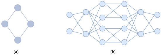
Figure 3.
Symmetric topologies for experiments: (a) 4 nodes with 8 agents; (b) 16 nodes with 64 agents.
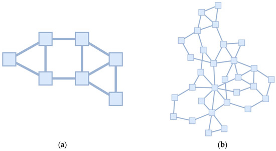
Figure 4.
Topologies from the TopologyZoo library: (a) Abilene—modified to reduce the number of transit vertices while preserving the asymmetry of the original topology. The final configuration contains 7 nodes and 20 agents; (b) Geant2009—with degree-1 vertices removed. The final configuration consists of 30 nodes and 96 agents.
Network load was represented by the set of flows, each as the tuple (source, destination, rate, and start/end time) and the scheduling of their beginnings. Flows were generated for average network loads of 40% or 60%.
The investigated algorithms and their parameters are specified in tabular form in Table 1 and in the following section.

Table 1.
Algorithm hyperparameter values.
Results were evaluated based on the objective function Φ (1) (also called solution quality) and the total number of agent exchanges.
To evaluate the optimality of obtained solutions, the results of experiments were compared with those of the centralized genetic algorithm. Although the genetic algorithm provided an approximate suboptimal solution to the NP-complete balancing problem—unlike the proposed method, it relied on a centralized view of all channel states—the values obtained through the genetic algorithm served as our benchmark. The genetic algorithm was selected, as it was applied for different network load-balancing problems [23,24].
The genetic algorithm with the objective to minimize the target function Φ was organized as follows. The crossover operation between two solutions (i.e., two sets of agent weights) worked as follows: over several iterations, Solution 1 and Solution 2 exchanged the weights of all agents at a randomly selected network node. The mutation operation involved multiple iterations where the weights of all agents at a randomly chosen node were cyclically shifted, followed by updating a random subset of these weights with new random values. Solution selection was performed based on the value of the objective function Φ.
The experiments were conducted under the assumption of synchronous switching between the layers to ensure the correct computation of the hidden state by each agent. Although this assumption is a restriction, our experiments show that, even with it, SAMAROH-2L still yields significant gains in both decision-making speed and a reduction in inter-agent communications. Removing this assumption is a promising direction for future research.
6. Experimental Results
6.1. MAROH vs. SAMAROH
In the first series of experiments, the effectiveness of simultaneous weight adjustments by all agents were compared with sequential ones where only a single agent performs actions. In Figure 5, Figure 6, Figure 7 and Figure 8, the comparison between MAROH and SAMAROH methods for the 4-node topology (Figure 3a) and Abilene topology (Figure 4a) under different load conditions is exhibited. On these figures solid lines represent the average Φ values over intervals of 2000–3000 episodes, while vertical bars indicate the range from minimum to maximum Φ values across these intervals. Single points to the right of the line plots mark the minimum values of Φ averaged over 2000-episode intervals.
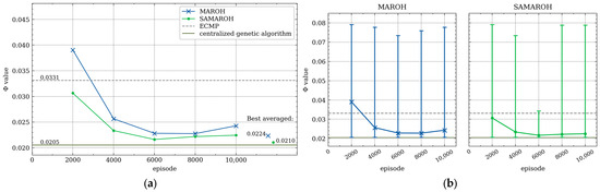
Figure 5.
Dependence of the objective function value on the episode number for MAROH and SAMAROH methods under 40% load for 4-node topology: (a) average values over 2000-episode intervals; (b) average values and min-max ranges over 2000-episode intervals.
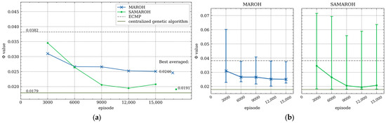
Figure 6.
Dependence of the objective function value on the episode number for MAROH and SAMAROH methods under 40% load for Abilene topology: (a) average values over 3000-episode intervals; (b) average values and min-max ranges over 3000-episode intervals.
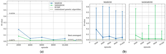
Figure 7.
Dependence of the objective function value on the episode number for MAROH and SAMAROH methods under 60% load for 4-node topology: (a) average values over 2000-episode intervals; (b) average values and min-max ranges over 2000-episode intervals.
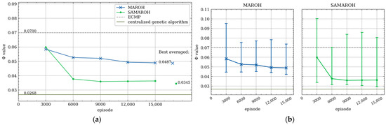
Figure 8.
Dependence of the objective function value on the episode number for MAROH and SAMAROH methods under 60% load for Abilene topology: (a) average values over 3000-episode intervals; (b) average values and min-max ranges over 3000-episode intervals.
In Figure 5, Figure 6, Figure 7 and Figure 8, the green line with a dot marker representing SAMAROH’s objective function values consistently remains below the blue one with a cross marker corresponding to MAROH’s performance. This phenomenon demonstrates that, despite all agents acting simultaneously, SAMAROH not only maintains almost the same quality, but also significantly improves it. This happens because the agents need to be trained to act in fewer horizons during an episode, which simplifies the training.
These figures also represent the results obtained with uniformed weights, representing traditional load-balancing approaches like ECMP. As evident across all plots, the green line with the dot marker (SAMAROH) consistently shows closer alignment with the centralized algorithm’s performance (indicated by a dark green solid horizontal line) compared to the gray dashed line representing ECMP.
SAMAROH required five times less horizons than the original MAROH (20 vs. 100 for the 4-node topology and 50 vs. 250 for Abilene). This translates to a fivefold reduction in both inter-agent communications and decision-making time, as achieving comparable results now requires significantly fewer horizons.
Conditions under which SAMAROH does not achieve a solution quality as good as MAROH were also examined. Table 2 presents a comparison of the objective function values for the Abilene topology under a 40% load for different values of trajectory lengths (PPO parameter which defines the period of neural network weights update) and Adam optimizer step size (parameter which controls the learning rate). Multiple values of optimizer step size were chosen, because different trajectory lengths may require different learning rates to achieve a solution of similar quality. The Φ values shown in Table 2 are derived as follows: for each experimental run, the average Φ value over the last 2000 episodes is calculated, and the average and standard deviation of such values from six independent runs (on different random seeds) is presented in the table. Optimizer step sizes are shown as a pair of values corresponding to actor and critic networks, respectively. The conclusion from Table 2 is that SAMAROH achieves a worse solution quality than MAROH on the trajectory length of 1 episode and a better quality length than MAROH on larger trajectory length, such as 5, 25, or 75 episodes (if choosing the optimizer step size that achieves the best solution quality among examined values). For all other experiments presented in this work, the trajectory length was chosen as 75 episodes, and Adam step sizes for experiments on Abilene topology were chosen as 0.00015 for the actor network and 0.00085 for the critic network.
Table 2.
Experimental comparison results of objective function of the proposed methods for Abilene topology with different values of trajectory length and optimizer step size over 8000 episodes.
6.2. Research of Two-Layer Approach
The next series of experiments were dedicated to evaluating of the efficiency of the two-layer approach. Figure 9, Figure 10, Figure 11 and Figure 12 present the comparison of this approach across all topologies, benchmarking the method against SAMAROH, the centralized genetic algorithm, and ECMP. In the legend, the two-layer method agent communication count (shown in parentheses) is expressed relative to SAMAROH’s baseline number of exchanges. In these series, the 4-node topology required the memory capacity for 512 states, while the other topologies required the memory capacity for 1024 states.
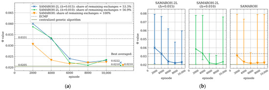
Figure 9.
Dependence of the objective function value on the episode number under 40% load for symmetric 4-node topology with 8 agents: (a) average values over 2000-episode intervals; (b) average values and min-max ranges over 2000-episode intervals.
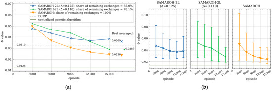
Figure 10.
Dependence of the objective function value on the episode number under 40% load for symmetric 16-node topology with 64 agents: (a) average values over 3000-episode intervals; (b) average values and min-max ranges over 3000-episode intervals.
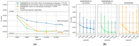
Figure 11.
Dependence of the objective function value on the episode number under 40% load for Abilene topology from TopologyZoo Library: (a) average values over 3000-episode intervals; (b) average values and min-max ranges over 3000-episode intervals.
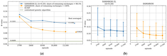
Figure 12.
Dependence of the objective function value on the episode number under 40% load for Geant2009 topology from TopologyZoo Library: (a) average values over 2700-episode intervals; (b) average values and min-max ranges over 2700-episode intervals.
In Figure 9, Figure 10, Figure 11 and Figure 12, the objective function values for SAMAROH-2L (shown as blue and green lines with cross and dot markers, respectively, for different proximity thresholds, except Figure 12 having only one threshold) consistently match or exceed the yellow line with an down arrow marker corresponding to SAMAROH’s performance.
The general conclusion from these results is as follows: with a moderate reduction in message exchanges (up to 20% for the Abilene topology, Figure 11), the two-layer method achieves objective function values that slightly differ from the SAMAROH ones. With more substantial reductions in exchanges, the two-layer method either yields significantly worse solution quality (for the Abilene topology, Figure 11) or requires more training episodes to match SAMAROH’s performance (for the 4-node topology, Figure 9). Meanwhile, the actual reduction in inter-agent exchanges can be adjusted between 25 and 50% depending on the required solution accuracy.
Figure 11 demonstrates that the proximity threshold Δ has significant impacts on the objective function value as on the number of inter-agent exchanges. Furthermore, the two-layer method’s performance is also under the influence of two key parameters: memory size and the comparison metric employed. The corresponding series of the experiments systematically evaluates the method efficacy across varying configurations of these parameters (see Table 3, Table 4 and Table 5).
Table 3.
Experimental comparison results of the proposed methods for the 4-node topology with 8 agents over 6000 episodes.
Table 4.
Experimental comparison results of the proposed methods for Abilene topology with 512 memory size over 15,000 episodes.
Table 5.
Experimental comparison results of the proposed methods for Abilene topology with 1024 memory size over 15,000 episodes.
Table 3 presents a comparison of the objective function values and exchange counts for the symmetric 4-node topology under a 40% load, while Table 4 and Table 5 show corresponding data for the Abilene topology at the same load level. Each reported value represents an average and standard deviation across six experimental runs on different random seeds. Due to computational constraints (with a single experiment involving 96 agents requiring over a week to complete), comprehensive parameter comparisons were not conducted for larger topologies. The Φ values shown in the tables correspond to the average over the last 2000 episodes of each experimental run. The amount of data exchanged per episode is calculated as an average by all the episodes, considering that, for each horizon, each agent exchanges from one to K messages with its neighbors four times (once for data collection and once for each training epoch). Each message occupies 64 bytes, since it represents the hidden state of an agent consisting of 16 real numbers. The number of exchanges between agents is given as a percentage relative to the number of exchanges in the corresponding single-layer method (that is, relative to MAROH for MAROH-2L and relative to SAMAROH for SAMAROH-2L).
For the 4-node topology, the memory size was fixed at 512 states based on the results from [11], representing the maximum capacity we could use to store representatives. As shown in Table 3, Φ values remain relatively stable at small threshold values, but the objective function begins to degrade as the threshold grows. This pattern is corresponded to the one in the Abilene topology results (Table 4 and Table 5). This is explained by the fact that, with an increasing threshold, states that correspond to different actions become close; however, the agent will apply the same action in both states. In the conducted series of experiments, the threshold value was set manually, but the question arises about an automatic method for selecting the value of this parameter in such a way that the compromise between the value of the objective function and the number of exchanges is observed.
It has to be kept in mind that the analyzed processes are non-stationary, and the observed values have very intricate interrelations. Under such conditions, the application of statistical tests will be unjustifiably redundant from the viewpoint of the correctness of statistical inferences for the area under consideration. It is extremely strange to expect that the strong theoretical conditions for the statistical tests to be adequate and hold in the area under consideration. It is either impossible to strictly verify the conditions of the tests’ adequacy or these tests conditions are obviously violated. For example, all sample elements (the values of the objective function) are positive and hence remain bounded from the left even after appropriate centering, whereas the normal distribution of the sample elements (assumed when the Student t-test is used) has the whole real line as its support (meaning that any non-empty interval must have the positive probability under the normal distribution). Therefore, when discussing the consistency of the obtained results, we are forcibly restricted to non-formal conclusions, for example, based on visual distinction or coincidence. Nevertheless, following the common practice in related studies (e.g., BayesIntuit [8]), we report the values of the corresponding statistical tests. For SAMAROH-2L on Abilene topology (for all metrics for 1024 memory size and L1 metric for 512 memory size) and MAROH-2L on 4-node topology, the increase in the objective function on higher thresholds was proven with the Student or Mann–Whitney U tests with p-values less than 0.05 (ranging from 5.8 × 10⁻⁵ to 0.024 for each set of thresholds), with samples consisting of 12—36 independent experiments. A more comprehensive exploration of these parameters is the important direction for future proposed method development.
The metric comparison across Table 3, Table 4 and Table 5 revealed that the L2 metric achieves a superior solution quality under the same number of exchanges.
For the Abilene topology, the memory size was set to 512 states (Table 4), consistent with the configuration in [11] for a comparable 4-node topology with similar agent numbers. Increasing the memory capacity to 1024 states (Table 5) while maintaining the same threshold has led to the downgrade of the objective. This can be explained by the fact that a larger number of representatives will have an intersection of Δ neighborhoods that can have different actions, which justifies the relevance of the method for selecting representatives without intersection of the Δ neighborhoods proposed in Section 4.2.3.
A comparison between MAROH-2L and SAMAROH-2L in Table 3 reveals that, while using identical memory parameters, SAMAROH-2L achieves a 30–70% reduction in message exchanges, whereas MAROH-2L only attains a 7–13% reduction. This performance gap likely stems from MAROH-2L’s fivefold greater number of horizons per episode, which proportionally generates more hidden states—consequently, the same memory size proves inadequate when compared to SAMAROH-2L’s requirements.
In Table 3, Table 4 and Table 5, the number of exchanges between agents for SAMAROH-2L is given as a percentage relative to the number of exchanges in SAMAROH. Since SAMAROH and SAMAROH-2L also have a reduction in the number of horizons in one episode relative to MAROH, the reduction in the number of exchanges in SAMAROH-2L relative to MAROH is much more significant. Thus, for Table 4 and Table 5, the number of horizons in one episode was reduced by five times; therefore, for example, the reduction in the number of communications to 80.06% relative to SAMAROH means that it was reduced to 0.8006 / 5 × 100% ≈ 16.01% relative to MAROH (this number ranges from 14.4% to 16.87% over different runs of the corresponding experiment). This reduction ratio can also be obtained by dividing values of exchanged data amounts for different algorithms in the tables.
In conclusion, the two-layer SAMAROH-2L method achieved significant improvements over the single-layer SAMAROH method: for the eight-agent topology, it reduced the objective function value from 0.0265 to 0.0236 while cutting communication exchanges by 40.92% (from 100% to 59.08% relative to the SAMAROH baseline), and for the Abilene topology, it reduced the objective function value from 0.0211 to 0.0208 while cutting communication exchanges by 19.94% (from 100% to 80.06% relative to the SAMAROH baseline).
7. Discussion
The efficiency of the proposed two-layer method was experimentally proven. This is especially clearly visible from the experiments with the Abilene topology, as the method maintained high-quality solutions (with the objective function reduced from 0.0211 to 0.0208) while achieving a 19.94% reduction in the number of communications relative to the corresponding single-layer method.
Promising directions for future research include
- Investigating the effectiveness of the representative selection method proposed in Section 4.2.3;
- Developing adaptive algorithms for state proximity threshold tuning;
- Creating dynamic memory management techniques with the intelligent identification of obsolete states and optimal memory sizing based on current network conditions;
- Study of channel quality indicators (e.g., delay, throughput, and packet loss) in large-scale topologies under high load using balancing by the proposed methods, as well as comparison with modern approaches;
- Optimizing computational complexity for large-scale network topologies.
A significant area of improvement for the method is the development of an adaptive algorithm for adjusting the state proximity threshold Δ. One possible approach is to calculate the maximum permissible number of representatives based on the available memory capacity and dynamically adjust the global threshold Δ. If the number of representatives exceeds the maximum allowable number, the threshold can be increased by merging representatives, provided that their associated actions are similar. A more sophisticated strategy could involve assigning individual thresholds to each representative based on the density of hidden states in the metric space. In dense regions, where similar states require different actions, a smaller threshold is beneficial. Conversely, in sparse regions, a larger threshold can be used to reduce memory consumption.
The current limitations of the method primarily involve extended training durations for 96-agent systems (necessitating distributed simulation frameworks) and the substantial number of required training episodes (4000–10,000). While accelerating multi-agent methods was not this study’s primary focus, it remains a crucial direction for future research.
While the proposed two-layer control architecture is developed and validated in the context of traffic engineering, its design principles—experience-based decision and collaborative problem-solving for novel states—might be possible to generalize to other cooperative multi-agent systems with similar characteristics (e.g., distributed control, partial observability, and communication constraints). However, further empirical validation in non-networking domains is needed to substantiate this potential.
8. Conclusions
A new multi-agent method for traffic flow balancing is presented based on two fundamental innovations: abandoning sequential models of agent decision-making and developing a two-layer human-like agent control plane in multi-agent optimization. For the agent control plane, the concept of agent hidden state representatives reflecting its experience was proposed. This concept has allowed to significantly reduce the number of stored hidden states. Two methods of representative selecting were proposed and investigated. Experimentally it was proven that the proposed innovations significantly reduce the amount of inter-agent communications, decision-making time by agents, and optimality of flow balancing while maintaining the original objective function.
The proposed method has significant potential for scalability, which is important for large-scale networks. Once a state representative is found in memory, action search is very efficient, requiring only a linear memory scan; this complexity can be further reduced to logarithmic time by using specialized data structures for similarity search, such as k-d trees. It should also be noted that when a representative for an agent’s state is not found, communication overhead remains limited, since the agent exchanges messages only within its k-hop neighborhood, without broadcasting them to the entire network. Moreover, since the method works by adjusting channel weights, data packets are never delayed for agent decisions and can continue to be forwarded using existing weights until new ones are calculated. A key question for future research is determining the optimal weight update frequency to minimize the duration of suboptimal routing while maintaining low communication overhead.
Author Contributions
E.S.: methodology, project administration, software, writing—original draft, and validation. R.S.: methodology, conceptualization, writing—review and editing, and supervision. I.G.: software, investigation, visualization, and formal analysis. All authors have read and agreed to the published version of the manuscript.
Funding
This work was supported by The Ministry of Economic Development of the Russian Federation in accordance with the subsidy agreement (agreement identifier 000000C313925P4H0002; grant No 139-15-2025-012).
Data Availability Statement
The original data presented in the study are openly available in Zenodo at https://doi.org/10.5281/zenodo.17208706.
Acknowledgments
We acknowledge graduate student Ariy Okonishnikov for his contributions to the initial implementation and preliminary experimental validation of the method.
Conflicts of Interest
The authors declare no conflicts of interest.
Abbreviations
The following abbreviations are used in this manuscript:
| CVDMARL | Communication-Enhanced Value Decomposition Multi-Agent Reinforcement Learning |
| Dec-POMDP | Decentralized Partially Observable Markov Decision Process |
| ECMP | Equal-Cost Multi-Path |
| GRU | Gated Recurrent Unit |
| LSTM | Long-Short-Term Memory |
| MARL | Multi-Agent Reinforcement Learning |
| MAROH | Multi-Agent Routing Using Hashing |
| MAROH-2L | MAROH with Two-Layer Control Plane |
| MLP | Multi-Layer Perceptron |
| MPNN | Message Passing Neural Network |
| NP | Non-deterministic Polynomial time |
| PPO | Proximal Policy Optimization |
| RL | Reinforcement Learning |
| SAMAROH | Simultaneous Actions MAROH |
| UCMP | Unequal-Cost Multi-Path |
References
- Moiseev, N.N.; Ivanilov, Y.P.; Stolyarova, E.M. Optimization Methods; Nauka: Moscow, Russia, 1978; 352p. [Google Scholar]
- Wang, I.L. Multicommodity network flows: A survey, Part I: Applications and Formulations. Int. J. Oper. Res. 2018, 15, 145–153. [Google Scholar]
- Wang, I.L. Multicommodity network flows: A survey, part II: Solution methods. Int. J. Oper. Res. 2018, 15, 155–173. [Google Scholar]
- Even, S.; Itai, A.; Shamir, A. On the complexity of time table and multi-commodity flow problems. In Proceedings of the 16th Annual Symposium on Foundations of Computer Science (sfcs 1975), Washington, DC, USA, 13–15 October 1975. [Google Scholar]
- Stepanov, E.P.; Smeliansky, R.L.; Plakunov, A.V.; Borisov, A.V.; Zhu, X.; Pei, J.; Yao, Z. On fair traffic allocation and efficient utilization of network resources based on MARL. Comput. Netw. 2024, 250, 110540. [Google Scholar] [CrossRef]
- Kahneman, D. Thinking, Fast and Slow; Macmillan: New York, NY, USA, 2011. [Google Scholar]
- Chang, A.; Ji, Y.; Wang, C.; Bie, Y. CVDMARL: A communication-enhanced value decomposition multi-agent reinforcement learning traffic signal control method. Sustainability 2024, 16, 2160. [Google Scholar] [CrossRef]
- Bornacelly, M. BayesIntuit: A Neural Framework for Intuition-Based Reasoning. In North American Conference on Industrial Engineering and Operations Management-Computer Science Tracks; Springer Nature: Cham, Switzerland, 2025; pp. 117–132. [Google Scholar]
- Ramani, D. A short survey on memory based reinforcement learning. arXiv 2019, arXiv:1904.06736. [Google Scholar] [CrossRef]
- Zheng, L.; Chen, J.; Wang, J.; He, J.; Hu, Y.; Chen, Y.; Fan, C.; Gao, Y.; Zhang, C. Episodic multi-agent reinforcement learning with curiosity-driven exploration. Adv. Neural Inf. Process. Syst. 2021, 34, 3757–3769. [Google Scholar]
- Okonishnikov, A.A.; Stepanov, E.P. Memory mechanism efficiency analysis in multi-agent reinforcement learning applied to traffic engineering. In Proceedings of the 2024 International Scientific and Technical Conference Modern Computer Network Technologies (MoNeTeC), Moscow, Russia, 29–31 October 2024. [Google Scholar]
- Kia, M.; Cramer, J.; Luczak, A. Memory Augmented Multi-agent Reinforcement Learning for Cooperative Environment. In International Conference on Artificial Intelligence and Soft Computing; Springer Nature: Cham, Switzerland, 2024; pp. 92–103. [Google Scholar]
- Yao, Z.; Ding, Z.; Clausen, T. Multi-agent reinforcement learning for network load balancing in data center. In Proceedings of the 31st ACM International Conference on Information & Knowledge Management, Atlanta, GA, USA, 17–22 October 2022; pp. 3594–3603. [Google Scholar]
- Bernárdez, G.; Suárez-Varela, J.; López, A.; Shi, X.; Xiao, S.; Cheng, X.; Barlet-Ros, P.; Cabellos-Aparicio, A. MAGNNETO: A graph neural network-based multi-agent system for traffic engineering. IEEE Trans. Cogn. Commun. Netw. 2023, 9, 494–506. [Google Scholar] [CrossRef]
- Sutton, R.S.; Barto, A.G. Reinforcement Learning: An Introduction; MIT Press: Cambridge, UK, 1998; Volume 1. [Google Scholar]
- Kryszkiewicz, M. The cosine similarity in terms of the euclidean distance. In Encyclopedia of Business Analytics and Optimization; IGI Global: Hershey, PA, USA, 2014; pp. 2498–2508. [Google Scholar]
- Xia, P.; Zhang, L.; Li, F. Learning similarity with cosine similarity ensemble. Inf. Sci. 2015, 307, 39–52. [Google Scholar] [CrossRef]
- Yosida, K. Functional Analysis; Springer Science & Business Media: Berlin/Heidelberg, Germany, 1995; Volume 123. [Google Scholar]
- Overview of Clustering Methods. Available online: https://scikit-learn.org/stable/modules/clustering.html#overviewof-clustering-methods (accessed on 5 August 2025).
- Peng, K.; Leung, V.C.M.; Huang, Q. Clustering approach based on mini batch kmeans for intrusion detection system over big data. IEEE Access 2018, 6, 11897–11906. [Google Scholar] [CrossRef]
- Garkavy, I. Estepanov-Lvk/Maroh: MAROH-2L V1.0.2. Zenodo. 2025. Available online: https://zenodo.org/records/17208706 (accessed on 26 September 2025).
- Topology Zoo. Available online: https://github.com/sk2/topologyzoo (accessed on 31 July 2025).
- Kang, S.-B.; Kwon, G.-I. Load balancing of software-defined network controller using genetic algorithm. Contemp. Eng. Sci. 2016, 9, 881–888. [Google Scholar] [CrossRef]
- Singh, A.R.; Devaraj, D.; Banu, R.N. Genetic algorithm-based optimisation of load-balanced routing for AMI with wireless mesh networks. Appl. Soft Comput. 2019, 74, 122–132. [Google Scholar] [CrossRef]
Disclaimer/Publisher’s Note: The statements, opinions and data contained in all publications are solely those of the individual author(s) and contributor(s) and not of MDPI and/or the editor(s). MDPI and/or the editor(s) disclaim responsibility for any injury to people or property resulting from any ideas, methods, instructions or products referred to in the content. |
© 2025 by the authors. Licensee MDPI, Basel, Switzerland. This article is an open access article distributed under the terms and conditions of the Creative Commons Attribution (CC BY) license (https://creativecommons.org/licenses/by/4.0/).