Quantum Computing Meets Deep Learning: A QCNN Model for Accurate and Efficient Image Classification

Abstract

In deep learning, Convolutional Neural Networks (CNNs) serve as fundamental models, leveraging the correlational structure of data for tasks such as image classification and processing. However, CNNs face significant challenges in terms of computational complexity and accuracy. Quantum computing offers a promising avenue to overcome these limitations by introducing a quantum counterpart-Quantum Convolutional Neural Networks (QCNNs). QCNNs significantly reduce computational complexity, enhance the models ability to capture intricate patterns, and improve classification accuracy. This paper presents a fully parameterized QCNN model, specifically designed for Noisy Intermediate-Scale Quantum (NISQ) devices. The proposed model employs two-qubit interactions throughout the algorithm, leveraging parameterized quantum circuits (PQCs) with rotation and entanglement gates to efficiently encode and process image data. This design not only ensures computational efficiency but also enhances compatibility with current quantum hardware. Our experimental results demonstrate the model’s notable performance in binary classification tasks on the MNIST dataset, highlighting the potential of quantum-enhanced deep learning in image recognition. Further, we extend our framework to the Wine dataset, reformulated as a binary classification problem distinguishing Class 0 wines from the rest. The QCNN again demonstrates remarkable learning capability, achieving 97.22% test accuracy. This extension validates the versatility of the model across domains and reinforces the promising role of quantum neural networks in tackling a broad range of classification tasks.

1. Introduction

Machine learning (ML) has revolutionized the way people interact with technology. As a crucial subfield of artificial intelligence (AI), ML enables computers to learn patterns from data autonomously rather than requiring explicit programming for each task [1,2]. Among the widely adopted ML models, neural networks stand out due to their adaptive learning capabilities, fault tolerance, self-organization, real-time processing, and parallelism [3]. Expanding on this foundation, deep learning enhances neural networks by incorporating multiple hidden layers, making them highly effective for handling vast amounts of data [4]. A prime example of this advancement is the Convolutional Neural Network (CNN), which excels at identifying patterns in data, making it highly effective for tasks such as image recognition and classification [5,6].

When designing Deep Neural Network (DNN) models, the primary objective is to optimize the network to achieve both high training accuracy and strong validation accuracy [7,8]. Training accuracy reflects the model’s performance on the training dataset, while validation accuracy measures how well the model generalizes to unseen data. A critical challenge in deep learning is ensuring good generalization, which determines how effectively a model adapts to new data. The generalization error (%) is defined as

$$\mathrm{Generalization}\mathrm{Error}(\%)={\displaystyle \frac{\mathrm{Train}\mathrm{Accuracy}-\mathrm{Validation}\mathrm{Accuracy}}{\mathrm{Train}\mathrm{Accuracy}}}\times 100$$

(1)

A high generalization error indicates that the model is overfitting-memorizing the training data rather than learning meaningful patterns-leading to poor performance on unseen data. Achieving the right balance between underfitting (low accuracy on both training and validation data) and overfitting is key to building robust deep learning models. Quantum computing [9] leverages principles of quantum mechanics, such as superposition and entanglement, to overcome the limitations of classical computing [10,11,12,13]. By exploiting these principles, quantum computing enables significantly faster computations for certain classes of problems. Quantum Machine Learning (QML), an emerging interdisciplinary field combining quantum computing and ML, has seen rapid advancements in recent years [14]. Traditional ML algorithms are typically composed of three key components: representation, evaluation, and optimization. In the quantum domain [15], research has primarily focused on advancing the evaluation process, which plays a crucial role in deep learning models [16]. QML shows particular promise for tasks where quantum computing can accelerate complex computations, such as image classification [17].

Quantum models offer significant advantages in image classification due to their inherent parallelism, rapid execution speed, and ability to drastically reduce the number of qubits required for encoding information compared to classical models. For example, with just 8 qubits, a 256-dimensional pattern can be represented, while only 30 qubits can encode a massive 32,768 × 32,768 binary image-equivalent to a flattened vector with over a billion dimensions. This remarkable compression is made possible through quantum superposition and entanglement, allowing for highly efficient data representation and processing.

Inspired by the success of CNNs and the potential of QML, researchers have developed Quantum Convolutional Neural Networks (QCNNs) [18,19,20]. Previous QCNN models have primarily taken two approaches: (1) designing efficient quantum arithmetic operations that replicate the core functions of classical CNNs or (2) developing parameterized quantum circuits (PQCs) inspired by CNN architectures. The first approach generally relies on fault-tolerant quantum hardware, while the second is mainly used for classifying quantum data.

In this study, we introduce a fully parameterized quantum circuit for QCNN, specifically designed for supervised classification tasks on classical data. PQCs are particularly well suited for Noisy Intermediate-Scale Quantum (NISQ) hardware [19]. Our framework systematically incorporates two-qubit interactions throughout the computational process while leveraging quantum entanglement-a key global quantum property-potentially surpassing the performance of classical CNNs. To evaluate our PQC-based QCNN, we conduct experiments on widely used datasets: MNIST and Wine dataset implemented using PennyLane [21]. The MNIST dataset consists of $28\times 28$ images of handwritten digits (0–9), and in this study, we focus on binary classification of digits 0 and 1. The wine dataset consists of three classes, with each class representing a wine made from a different grape variety. And we just identify whether a wine is from Class 0 or not (which includes both Class 1 and Class 2). Our findings indicate that QCNNs can outperform classical models in certain scenarios, highlighting their potential advantages over traditional deep learning approaches [22].

1.1. Motivation and Research Contribution

Recent studies highlight the promise of integrating quantum computing with classical machine learning techniques across various tasks [23,24,25]. These hybrid approaches show considerable potential, yet challenges remain. Further advancements are needed in optimization techniques, circuit architectures, and scalability to larger qubit systems to fully leverage the power of quantum computing in enhancing machine learning models [26]. The subsequent delineates the contributions of the proposed work:

• This study presents a fully Quantum Convolutional Neural Network (QCNN) model designed specifically for binary classification on the MNIST focusing on distinguishing between digits 0 and 1. We further extend to the classification of the wines by analyzing the wine dataset. While previous approaches often rely on either classical deep learning models or hybrid quantum-classical structures, our work explores a purely quantum model that is both compact and efficient.
• One of the main contributions is the design of a shallow QCNN architecture that operates on small subsets of qubits at each layer. This avoids the use of deep parameterized quantum circuits, which are prone to noise and training instability, particularly on current quantum hardware. By keeping the circuit depth low and the architecture modular, we ensure better trainability and scalability.
• We also introduce a specific quantum unitary block based on a combination of Ry, Rz, U3, and CNOT gates. These blocks form the building units of our convolutional layers and together include only 45 trainable parameters in total. This efficient gate design reduces resource consumption while maintaining expressivity.
• Despite the simplicity of the architecture, our model achieves an accuracy of 97.26% on the MNIST dataset binary classification task and 97.22% in the classification of wine by analyzing the wine dataset. Our results shows that the proposed approach is still competitive and demonstrate the potential of quantum inspired methods for practical classification tasks. We also provide a computational analysis to show how our model compares favorably in terms of parameter count, gate complexity, and memory requirements.
• Altogether, this work demonstrates that a carefully structured shallow quantum model can perform competitively with more complex alternatives, making it a promising candidate for practical use on near-term quantum hardware.

1.2. Organization

The structure of this study is as follows: Section 2 comprises the review of the literature in the field of quantum computing and QML in image classification. Section 3 comprises some models’ performance on the datasets used. Section 4 consists of the fundamental concepts of quantum computing and some QML techniques. Section 5 covers detailed analysis of the dataset and the model’s experimental setup. Section 6 describes the performance matrices that evaluate the performance of our classification model. Section 7 offers an evaluation of our QCNN framework. Section 8 concludes the article and outlines potential future research and development directions.

2. Related Work

2.1. Convolutional Neural Network

The development of the Neocognitron in 1980 [27] introduced hierarchical layers for feature extraction, laying the foundation for Convolutional Neural Networks (CNNs). In 1989, LeCun et al. introduced a CNN [28], which became essential for image classification tasks. Later, LeCun and colleagues introduced LeNet-5 [29], a CNN designed for digit recognition tasks, particularly for handwritten ZIP code classification using the MNIST dataset. LeNet-5 incorporated key CNN components, such as convolutional layers, pooling layers, and fully connected layers, which form the core structure of modern CNNs.

The resurgence of interest in neural networks, fueled by advances in deep learning, led to the systematic development of various CNN models. A significant breakthrough came in 2012 when Krizhevsky et al. proposed AlexNet [30], a deep CNN model that won the ImageNet Large Scale Visual Recognition Challenge (ILSVRC). AlexNet introduced ReLU activations, dropout layers, and GPU-based training, making CNNs practical for large-scale applications.

Further advancements in CNN architectures resulted in improved models such as VGG [31], GoogleNet [32], and ResNet [33]. Modern CNN innovations include DenseNet [34], which introduced dense connections, allowing each layer to receive input from all preceding layers, thereby enhancing gradient flow and optimizing parameter efficiency.

Several studies have compared the image detection abilities of trained neural networks with those of human subjects. Results indicate that while humans achieve an accuracy of 73.1% on specific datasets, a trained neural network performs slightly lower at 64%. However, when CNNs were applied to the same dataset, they achieved an accuracy of 74.9%, surpassing human performance [35]. Ongoing studies continue to explore the behavior of Deep Neural Networks in different scenarios [36].

Karpathy et al. [37] trained a CNN model on a massive dataset consisting of one million YouTube videos covering 487 classes. Their study demonstrated CNNs’ ability to extract robust features from large-scale, noisy, and weakly labeled data, achieving a performance boost of up to 63.3% in classifying 50 clips from every video. Similarly, Neha et al. [38] presented a performance analysis of CNNs on CIFAR-10 and CIFAR-100 datasets in ICCIDS 2018. Jmour et al. [39] trained a CNN for traffic sign classification using the ImageNet dataset, achieving a 93.3% accuracy using a batch size of 10. Drishti et al. [40] recognized handwritten digits from the MNIST dataset using both Artificial Neural Networks (ANNs) and CNNs, achieving a 1.31% baseline error for ANN and a 0.91% baseline error for CNN after training 60,000 images with an epoch value of 10 and a batch size of 200. (Summarised in

Table 1. Related work in CNN development.

Reference	Technique Used	Highlights	Limitations
Fukushima (1980) [27]	Neocognitron	Introduced hierarchical layers for feature extraction, laying the foundation for CNNs.	Did not fully address scalability and complex dataset generalization.
LeCun (1989) [28]	CNN	Essential for image classification tasks using backpropagation.	Limited computational power restricted its adoption.
LeCun et al. (1998) [29]	LeNet-5	Designed for handwritten ZIP code recognition on MNIST; incorporated convolution, pooling, and fully connected layers.	Restricted to digit classification, lacked generalization to broader datasets.
Krizhevsky et al. (2012) [30]	AlexNet	Introduced ReLU, dropout, and GPU training; won ILSVRC 2012.	Large parameter count; prone to overfitting on smaller datasets.
Simonyan & Zisserman (2014) [31]	VGG	Used deeper architectures with smaller filters, improving accuracy.	High memory and computational costs.
Szegedy et al. (2015) [32]	GoogleNet	Introduced Inception modules for efficient feature extraction.	Complex design; less flexible for modifications.
He et al. (2016) [33]	ResNet	Introduced residual learning to solve vanishing gradient problem.	Overhead in very deep networks; risk of overfitting.
Huang et al. (2017) [34]	DenseNet	Dense connections improved gradient flow and parameter efficiency.	Increased memory requirements.
Yang et al. (2015) [35]	CNNs vs. Humans	CNNs achieved 74.9% accuracy vs. humans’ 73.1%, surpassing human performance.	Limited to specific datasets; generalization uncertain.
Karpathy et al. (2014) [37]	CNN on YouTube videos	Trained on 1M videos, extracted robust features, achieved 63.3% accuracy.	Weakly labeled data; noisy dataset.
Neha et al. (2018) [38]	CNN (CIFAR-10/100)	Performance analysis on standard datasets.	Dataset-specific evaluation; lacks generalization insights.
Jmour et al. (2018) [39]	CNN (Traffic Signs)	Achieved 93.3% accuracy on ImageNet with batch size 10.	Smaller batch size may affect scalability.
Drishti et al. (2021) [40]	ANN vs CNN (MNIST)	ANN: 1.31% baseline error; CNN: 0.91% error (60 k images, 10 epochs, batch size 200).	Limited to handwritten digits; not tested on more complex datasets.

).

2.2. Quantum Machine Learning

The integration of quantum principles into machine learning techniques has led to significant research in the Quantum Machine Learning (QML) domain. Quantum Support Vector Machine (QSVM) was proposed by Patrick Rebentrost for classification tasks [41]. In 2015, Ostaszewski et al. introduced a quantum-based algorithm applying Principal Component Analysis (PCA) for pattern recognition in images [42]. Ruan et al. [43] introduced a quantum algorithm for a classical K-Nearest Neighbors (KNNs) method, designing a quantum computing model to compute the Hamming distance between a test sample and the training set feature vectors (Summarised in

Table 2. Related work in Quantum Machine Learning (QML).

Reference	Technique Used	Highlights
Rebentrost et al. [41]	Quantum Support Vector Machine (QSVM)	Proposed QSVM for classification tasks, demonstrating the potential of quantum speedup in supervised learning.
Ostaszewski et al. [42]	Quantum Principal Component Analysis (QPCA)	Introduced a quantum-based algorithm applying PCA for image pattern recognition.
Ruan et al. [43]	Quantum K-Nearest Neighbors (QKNNs)	Developed a quantum algorithm inspired by classical KNN, efficiently computing Hamming distance between test samples and training vectors.

).

2.3. Quantum Convolutional Neural Network (QCNN)

QCNN emerges as an integrated branch of quantum computing and deep learning, utilizing the hierarchical structure of CNNs with quantum circuits and entanglement to process quantum and classical data efficiently. QCNN was first proposed by Cong et al. (2019) [44], inspired by classical CNNs. They introduced a hierarchical quantum circuit that utilized Parameterized Quantum Circuits (PQCs) for data representation learning, quantum-based downsampling for reducing dimensionality, and quantum entanglement. This model was effective in classifying quantum states and addressing quantum many-body problems. Researchers have explored the QCNN approach for efficiently classifying classical image data. Henderson et al. [22] trained QCNNs for handwritten digit classification using the MNIST dataset. They introduced the concept of a quanvolutional layer, a quantum analog to classical convolutional layers, showing that integrating quantum circuits into neural network architectures enhances feature extraction and improves classification-performance.

Kerenidis et al. [45] proposed a quantum approach to building and training deep CNNs with the potential for significant speed improvements over classical methods. Their QCNN model incorporated key CNN features, including non-linear activations and pooling layers. Numerical simulations using the MNIST dataset demonstrated the practical viability of their model. Li et al. [46] explored a quantum adaptation of deep CNNs for image recognition. Their method involved preprocessing image data using hierarchical quantum renormalization and fractal-based scaling techniques, leading to improved efficiency and accuracy in recognizing images. Their findings suggest that QCNNs, paired with specialized feature extraction methods, can outperform conventional deep learning models. Hur et al. [47] improved quantum encoding techniques for processing classical images more effectively. They introduced a quantum neural network model designed to operate using only two-qubit interactions. Their study evaluated different QCNN models based on quantum circuit structures, data encoding techniques, classical preprocessing, cost functions, and optimization methods, testing them on MNIST and Fashion MNIST datasets. Yousif et al. [48] explored how quantum computing enhances image classification. Their QCNN model overcame limitations of traditional CNNs, particularly in computational efficiency and generalization. By incorporating quantum circuits for convolution and pooling operations, their model effectively handled high-dimensional data, demonstrating the flexibility of quantum circuits in feature extraction. Hassan et al. [49] introduced a QCNN-based approach to biomedical image classification. Their hybrid model combined QCNNs with a modified ResNet50 architecture to improve classification accuracy on medical image datasets, highlighting the potential of quantum computing in advancing medical image analysis (Summarised in

Table 3. Related work on Quantum Convolutional Neural Networks (QCNNs).

Reference	Focus	Highlights
Cong et al. (2019) [44]	Foundational QCNN	Proposed QCNN inspired by classical CNNs; introduced hierarchical PQCs, quantum downsampling, and entanglement. Effective in classifying quantum states and solving many-body problems.
Henderson et al. (2020) [22]	Quanvolutional Layer	Developed QCNN for MNIST classification. Introduced quanvolutional layer, showing quantum circuits enhance feature extraction and classification accuracy.
Kerenidis et al. (2019) [45]	Deep QCNN with speedup	Proposed quantum approach to deep CNNs with non-linear activations and pooling. Numerical simulations on MNIST showed practical viability and speed improvements.
Li et al. (2020) [46]	Quantum Image Recognition	Applied hierarchical quantum renormalization and fractal-based scaling for image recognition. Demonstrated efficiency and accuracy gains in QCNN-based models.
Hur et al. (2022) [47]	Quantum Encoding & Optimization	Proposed QCNN with two-qubit interactions. Compared models based on circuit structures, encoding, preprocessing, cost functions, and optimization. Tested on MNIST and Fashion-MNIST.
Yousif et al. (2024) [48]	Enhanced QCNNs	Showed QCNNs overcome CNN limitations in efficiency and generalization. Used quantum circuits for convolution/pooling to handle high-dimensional data effectively.
Hassan et al. (2024) [49]	Biomedical QCNN	Proposed hybrid QCNN + ResNet50 model for medical image classification, achieving improved accuracy and highlighting QCNN’s potential in healthcare.

).

3. Performance of Neural Network Models in Classification

Here, we present the performance of several neural network models that have been applied to the classification of the MNIST dataset. Syed et al. [50], in their paper “A Systematic Literature Review on Binary Neural Networks”, examined a variety of models that exploit different datasets and achieve improved performance accuracies [51,52,53,54]. Models that are applied to the MNIST dataset are also summarized in

Table 4. Performance of different models on the dataset.

Reference	Model Used	Dataset	Accuracy (%)
[51]	CNN	MNIST	96
[52]	BNN	MNIST	96.1
[53]	Binary-Memristor Crossbar	MNIST	91.7
[54]	1T1DM Architecture	MNIST	89.34
[55]	CNN (LeNet-5)	MNIST	94.0
[56]	CNN	MNIST	96.5
[57]	SVM	MNIST	95.88
[58]	QNN	WINE	75–85

.

Wu et al. [55] worked on digit recognition using the MNIST dataset and reported an accuracy of approximately 94% with the LeNet-5 architecture, a convolutional neural network (CNN) model, which represents a strong baseline performance. Cohen et al. [56] conducted a comparative study between the NIST and MNIST digit classification tasks, reporting an accuracy of around 96.5% on MNIST digit recognition. Similarly, Gope et al. [57] applied machine learning techniques to identify handwritten digits from the MNIST dataset. By employing a Support Vector Machine (SVM) classifier, they achieved an accuracy of 95.88%. Qian et al. [58] in their study tackled the full multiclass classification problem (distinguishing between all three wine cultivars) and reported only about 75–85% accuracy with quantum models.

It is important to note that in some cases, models may fail to learn effectively, resulting in stagnation of accuracy improvements. Such challenges can limit the ability to achieve the desired performance levels. In our work, first we focus on the binary classification of the MNIST dataset and further extend validation to the Wine dataset. Our model achieves an accuracy of 97.26% in the binary classification of MNIST digits, demonstrating a good performance on this dataset. Then, it focuses on a simplified binary classification task specifically, identifying whether a wine belongs to Class 0 or not, which reduces the complexity of the learning process and leads to achieving a high 97.22% accuracy on the Wine dataset. We also wisely selected just 8 out of the 13 features in the dataset to match our eight-qubit circuit, keeping the model efficient and more suitable for quantum processing. Moreover, our use of modern optimization techniques like the Adam optimizer and a well-structured QCNN circuit helped the model converge quickly and generalize well.

4. Preliminaries

The fundamental indivisible component of any physical system is termed as the quantum. Some special phenomena of quantum mechanics include superposition, entanglement, quantum parallelism, quantum confinement, and qubits. When processing is based on the core principles of quantum mechanics, it is referred to as quantum computing [59]. Integrating quantum mechanics with computational methodologies enables tackling complex tasks rapidly and accurately. A qubit is the fundamental unit of quantum information, analogous to the classical bit but with an essential difference: it can exist in a superposition of states [60,61]. Mathematically, a qubit is denoted as

$$|\psi \rangle =C_0|0\rangle +C_1|1\rangle$$

(2)

where $C_0$ and $C_1$ are complex probability amplitudes satisfying the normalization condition $|C_0{|}^2+{\left|C_1\right|}^2=1$ [62]. Upon measurement, the qubit collapses into either |0〉 or |1〉 with probabilities $|C_0{|}^2$ and $|C_1{|}^2$, respectively. Qubits can be implemented using superconducting circuits, trapped ions, and photonic systems. The geometrical representation of Equation (2) through polar coordinates [63] $\theta$ and $\varphi$ is given as

$$|\psi \rangle =cos\left({\displaystyle \frac{\theta }{2}}\right)|0\rangle +e^{i\varphi }sin\left({\displaystyle \frac{\theta }{2}}\right)|1\rangle$$

(3)

Here, the coefficients are determined by the polar angle (zenith angle) $\theta$ and azimuthal angle $\varphi$, where $0\le \theta \le \pi$ and $0\le \varphi \le 2\pi$. The Bloch sphere provides a geometric interpretation of quantum state evolution and gate operations [64,65]. The depiction of a single qubit state on a three-dimensional unit sphere is termed the Bloch sphere. Angles $\theta$ and $\varphi$ define the orientation of the qubit on the sphere. The Bloch vector $\mathbf{r}$ represents a qubits state as a point on the Bloch sphere in three-dimensional space, defined as

$$\mathbf{r}=(r_x,r_y,r_z)$$

(4)

where the components are given by the expectation values of the Pauli matrices:

$$r_x=\langle {\sigma }_x\rangle ,r_y=\langle {\sigma }_y\rangle ,r_z=\langle {\sigma }_z\rangle .$$

(5)

The Bloch vector is associated with the density matrix $\rho$ of a qubit as

$$\rho ={\displaystyle \frac{1}{2}}(I+\mathbf{r}·\mathbf{\sigma })$$

(6)

where $\mathbf{\sigma }=({\sigma }_x,{\sigma }_y,{\sigma }_z)$. For a pure state, the Bloch vector lies on the surface of the Bloch sphere ($\left|\mathbf{r}\right|=1$), while for a mixed state, it lies inside ($\left|\mathbf{r}\right|\le 1$).

A multi-qubit system is essentially a combination of multiple single qubits, meaning it can exist in a linear combination of all possible states, spanning from $|00\dots 00\rangle$ to $|11\dots 11\rangle$ simultaneously. This operation exploits the quantum mechanical property of entanglement. Entanglement is a crucial property that establishes correlations between qubits. It means that two entangled quantum states cannot be decomposed into independent states. If $|{\psi }_{XY}\rangle$ is a two-qubit entangled state, then it cannot be expressed as the tensor product of its individual components $|{\psi }_X\rangle$ and $|{\psi }_Y\rangle$:

$$|{\psi }_{XY}\rangle \ne |{\psi }_X\rangle \otimes |{\psi }_Y\rangle$$

(7)

Before executing a quantum algorithm, classical data must be converted into a quantum state, a process known as information encoding. This step is crucial for utilizing quantum computation effectively. The three main encoding techniques are discussed in Section 4.3.

4.1. Quantum State Transformation

Once data are encoded into a quantum state, the next step in quantum computing is state transformation. This process is essential for performing computations and requires executing a sequence of quantum gates to manipulate qubits. These gates modify the quantum state through operations like rotation, entanglement, and phase shifts, tailoring it for specific computational tasks. Quantum gates function similarly to logic gates in classical computers, but with a key distinction: they must be unitary, meaning they preserve the systems normalization and reversibility. This ensures that quantum computations remain coherent and can be reversed when needed. Fundamental quantum gates used in this article for computations include $R_X,R_Y,$ and $R_Z$ gates. These rotation gates manipulate qubits along the X, Y, and Z axes, in sequence, enabling precise control over quantum states. A Controlled Not (CNOT) gate is a two-qubit gate that invert the state of a target qubit if the control qubit is in the |1〉 state, creating entanglement. $U_3$ gate: a versatile, parameterized gate that applies a rotation using three Euler angles, providing full control over a qubit’s state. By strategically applying these quantum gates, quantum computers can manipulate qubits to perform complex calculations that classical computers would struggle to handle efficiently. Matrix representation of these elementary quantum gates are shown in

Table 5. Matrix representation of quantum gates used in this study.

$R_x\left(\mathit{\theta }\right)=\left[\begin{array}{cc}cos\frac{\mathit{\theta }}{2}& -isin\frac{\mathit{\theta }}{2}\\ -isin\frac{\mathit{\theta }}{2}& cos\frac{\mathit{\theta }}{2}\end{array}\right]$,	$R_y\left(\mathit{\theta }\right)=\left[\begin{array}{cc}cos\frac{\mathit{\theta }}{2}& -sin\frac{\mathit{\theta }}{2}\\ sin\frac{\mathit{\theta }}{2}& cos\frac{\mathit{\theta }}{2}\end{array}\right]$,	$R_z\left(\mathit{\theta }\right)=\left[\begin{array}{cc}{e}^{-i\mathit{\theta }/2}& 0\\ 0& e^{i\mathit{\theta }/2}\end{array}\right]$
$CNOT=\left[\begin{array}{cccc}1& 0& 0& 0\\ 0& 1& 0& 0\\ 0& 0& 0& 1\\ 0& 0& 1& 0\end{array}\right]$,   $U3(\theta ,\varphi ,\lambda )=\left[\begin{array}{cc}cos{\displaystyle \frac{\theta }{2}}& -e^{i\lambda }sin{\displaystyle \frac{\theta }{2}}\\ e^{i\varphi }sin{\displaystyle \frac{\theta }{2}}& e^{i(\varphi +\lambda )}cos{\displaystyle \frac{\theta }{2}}\end{array}\right]$

.

4.2. Quantum Measurement

Measurement is the final step in a quantum circuit, where the quantum state is observed and transformed into classical data. This process extracts useful information from the quantum system, such as expectation values, which can serve as the computational results of a quantum algorithm.

In this study, we utilize expectation values as key features derived from input images, which are then used for further classification.

In the context of QML, PQCs are widely used in quantum-classical approaches [66,67]. A PQC consists of fixed quantum gates with adjustable parameters fine-tuned throughout training. While a conventional computer handles the optimization process, the quantum machine executes state transformations and measurements, making use of quantum properties to enhance learning capabilities.

4.3. Data Encoding

Machine learning relies heavily on large datasets to train models effectively. However, in the current NISQ era, the number of available qubits is extremely limited, and diverse quantum-native datasets are scarce. As a result, researchers primarily use classical datasets, which must be encoded into quantum states for processing by QML algorithms, such as quantum neural networks. In simple terms, data encoding involves converting classical data points into quantum states so they can be manipulated within a quantum system. This process is achieved using a unitary state preparation circuit [68], denoted as S(x), which implements a sequence of single- and two-qubit gates to transform an initial quantum state typically the all zero state into a meaningful representation of the data. This encoding step is essential for enabling quantum models to learn from and process classical data efficiently. Mathematically, this is expressed as

$$E\left(x\right)=S_x{|0\rangle }^{\otimes n}$$

(8)

The inverse operation, $S_x^{†}$, can also be used to retrieve the encoded data. For S(x) to be efficient and practical for quantum data encoding, two main conditions must be met:

1.

Polynomial Complexity: The number of quantum gates required for encoding should increase at a polynomial or sub-polynomial rate as the number of qubits expands. If the gate count grows exponentially, the encoding becomes impractical.

2.

Hardware Efficiency: The state preparation circuit should be designed so that single- and two-qubit quantum gates can be implemented efficiently, without introducing excessive hardware costs or increasing error rates.

Efficient encoding ensures that Quantum Machine Learning models can process large datasets effectively while maintaining computational feasibility within the limitations of current quantum hardware.

Multiple techniques exist for embedding data into an n-qubit quantum system [69], each with unique characteristics and applications. Some of the most common techniques include amplitude encoding, angle encoding, and basis encoding. In this discussion, we focus on amplitude encoding and angle encoding, since they are among the highly used approaches and angle encoding is the one which is utilized in our study. These methods allow for efficient encoding of classical information into quantum states, making them essential for Quantum Machine Learning and quantum computing applications.

4.3.1. Amplitude Encoding

Amplitude encoding is a method for encoding classical information, like a numerical vector, onto the quantum state amplitudes. This technique is highly efficient because it allows $2^n$ classical values to be represented using only n qubits, providing an exponential advantage in data storage. Mathematically, a normalized classical vector $x\in {\mathbb{C}}^{2^n}$(where ${\left|\right|x\left|\right|}^2=1$) can be mapped onto a quantum state in the following manner:

$$|x\rangle =\sum _{j=1}^{2^n}{x}_j|j\rangle$$

(9)

• $x_j$ are the amplitude coefficients that define the likelihood of observing the corresponding basis state |j〉.
• Each basis state |j〉 represents one possible fundamental state in an n-qubit quantum framework.

For a given normalized classical matrix M of dimensions $2^m\times 2^n$ in the complex space $C^{2^m}\times C^{2^n}$, where the sum of the squared elements is 1,

$$\sum _{i=1}^{2^m}\sum _{j=1}^{2^n}{\left|a_{ij}\right|}^2=1$$

(10)

This matrix can be encoded into a quantum state as

$$|M\rangle =\sum _{i=1}^{2^m}\sum _{j=1}^{2^n}{a}_{i}j|i\rangle |j\rangle$$

(11)

Amplitude encoding for matrices is a powerful way to embed classical information into quantum states by expanding the Hilbert space. This method enables quantum computers to process large datasets efficiently but comes with practical challenges in state preparation and hardware limitations.

4.3.2. Angle Encoding

In angle-based encoding, classical features are encoded into the quantum gate rotation parameters that act on individual qubits. Qubits are initialized to |0〉 and parametrized quantum gates ($R_x\left(\theta \right),R_y\left(\theta \right),R_z\left(\theta \right)$) and the general unitary gate $U_3(\theta ,\varphi ,\lambda )$ (as given in Table 5) are applied to prepare the desired quantum state. Classical image data are transformed into a quantum state in the following manner:

• Rescaling pixel values: Since pixel intensity values typically range from 0 to 1 (after normalization), they are mapped to the range [0,$2\pi$] for quantum encoding.
• Calculation of the rotation angle: Given a pixel value $C_{xy}$ at position (x, y), the corresponding rotation angle $\theta$ is computed as

  $${\theta }_i=\pi .C_{xy}$$

  (12)
• Application of the rotation gate: Each qubit is assigned to one pixel and is rotated using the $R_y\left(\theta \right)$ gate.
• Final quantum state representation: Using n qubits, the resulting quantum state obtained by applying the gate to each qubit is

  $$|\psi \rangle =\underset{i=1}{\overset{n}{⨂}}U({\theta }_i,{\varphi }_i,{\lambda }_i){|0\rangle }^{\otimes n}$$

  (13)

  •

  n is the number of qubits (equal to the number of pixels).

  •

  ${\theta }_i=\pi C_i$ (rescaled classical data feature).

  •

  ${\varphi }_i$ and ${\lambda }_i$ can be fixed values or additional learnable parameters.

  •

  ${|0\rangle }^{\otimes n}$ denotes the initial zero state of all qubits before encoding.

Typically, ${\varphi }_i$ and ${\lambda }_i$ are set at 0 for standard angle encoding, unless additional phase control is needed.

This simplifies the unitary gate to

$$U({\theta }_i,0,0)=\left[\begin{array}{cc}cos({\theta }_i/2)& sin({\theta }_i/2)\\ -sin({\theta }_i/2)& cos({\theta }_i/2)\end{array}\right]$$

(14)

4.4. CNN and QCNN

Classical Convolutional Neural Networks (CNNs) have revolutionized image processing by efficiently identifying patterns and features through convolution and pooling layers. Classical convolution works by moving a filter across an image to pick out features like edges or textures; quantum convolution takes a different route. QCNN uses the unique properties of quantum systems-like entanglement and superposition-to process data in a more abstract way. In a Quantum Convolutional Neural Network (QCNN), groups of qubits are entangled and manipulated using quantum gates, allowing the network to focus on small patches of data at a time, just like classical filters do. These patches are then combined or measured to reduce the overall size of the data, similar to pooling layers in regular CNNs. Quantum filters are special because they can capture complex, non-local patterns in data that classical filters find difficult to handle. This can lead to more powerful and compact models, especially for tasks involving structured or low-dimensional input.

This fusion of classical and QML methods opens the door to enhanced image recognition, pattern detection, and classification, offering promising improvements in performance as quantum technology continues to evolve [70,71]. The general architecture of CNNs and QCNNs is depicted in Figure 1 and Figure 2, respectively.

4.5. Computational Efficiency and Challenges in QCNN

One of the exciting things about QCNNs is that they have the potential to achieve more with less, especially when it comes to computation. Especially with deep CNNs, the number of parameters and operations can quickly become massive as the model or input data grows. That means training them can take a lot of time, memory, and powerful hardware like GPUs.

In our quantum model, there are three convolutional layer, each using a sequence of parameterized gates grouped as $U_{SU}$, with each unitary comprising 15 gates. In the first, second, and third layers, this unitary is applied seven, four, and one times, respectively, resulting in a total of twelve gate blocks per forward pass. Thus, each prediction involves approximately 180 quantum gates, maintaining a relatively shallow circuit depth which aids both simulation efficiency and resilience to quantum noise.

Training quantum models is computationally intensive, as gradients are calculated using the parameter-shift rule that requires two circuit executions per trainable parameter. With 45 parameters and 25 samples per batch, one training step requires about 2250 circuit runs. Over the full 100-step training process, this results in approximately 225,000 quantum circuit executions.

Simulations were conducted using PennyLane’s default.qubit backend, which relies on a statevector approach. Memory consumption scales exponentially with the number of qubits: for 8 qubits, the statevector consists of $2^8=256$ complex amplitudes, consuming roughly 4 KB. As the qubit count increases, e.g., to 20 qubits, the memory demand surges to over 16 MB, making simulations beyond 30 qubits infeasible on typical machines.

If we talk about how well a QCNN performs, it’s not just about the accuracy number, it is also important to understand where things can go wrong. QCNNs have shown encouraging results, especially on small or well-structured datasets and binary classification tasks. But when it comes to more complex, high-resolution data, they can still fall behind their classical counterparts. That is mostly because today’s quantum hardware is not yet powerful or stable enough for large-scale tasks. But as quantum computers improve, QCNNs could become a much faster and more efficient way to solve certain types of problems.

5. Material and Methodology

5.1. Dataset Preparation

1.

MNIST

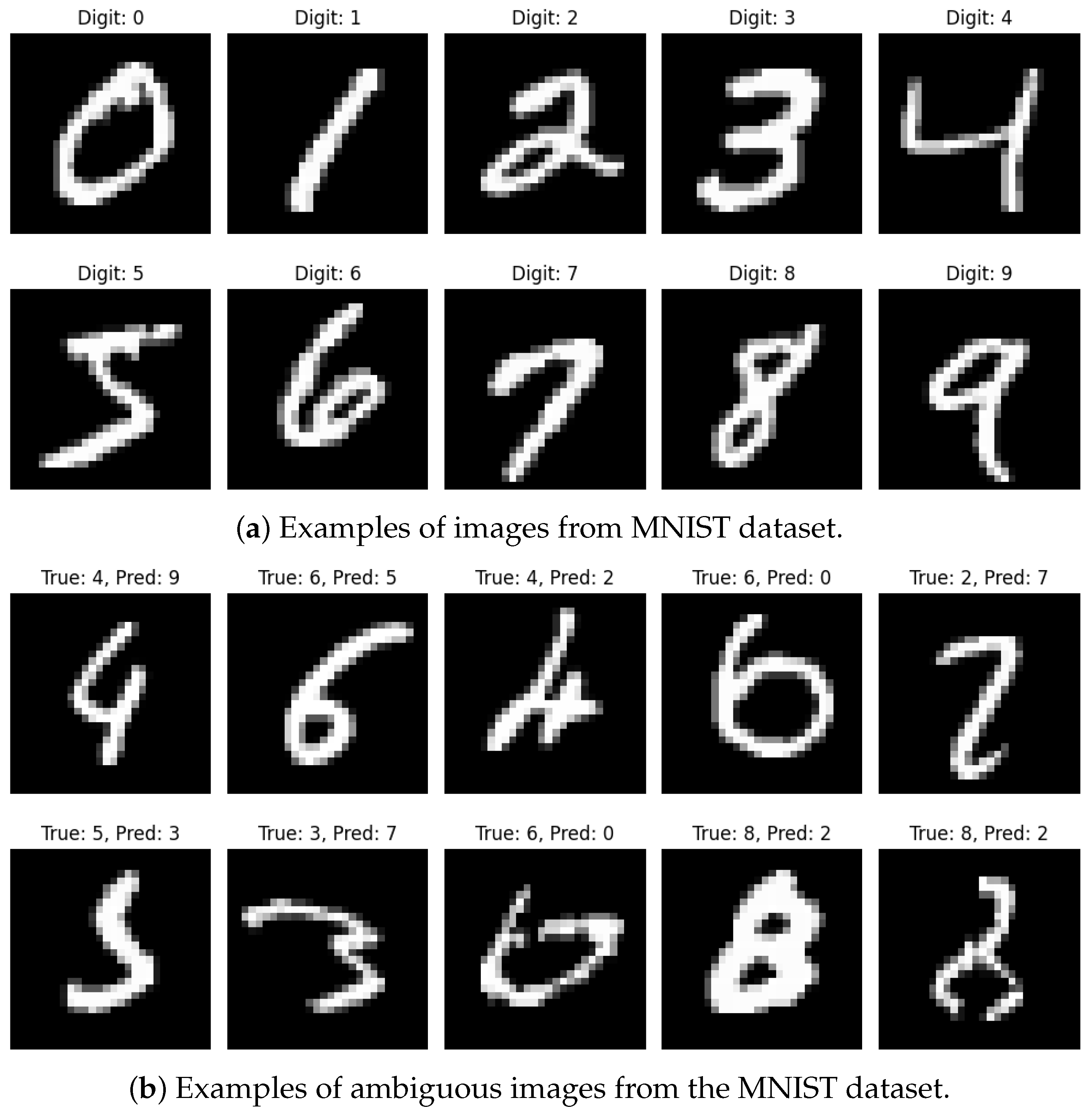
The Modified National Institute of Standards and Technology (MNIST) dataset is a widely recognized set of grayscale images showcasing handwritten digits spanning from 0 to 9. This dataset comprises a total of 70 K images, with 60 K allocated for model training and the remaining 10 K reserved for evaluation. Each image has a resolution of 28 × 28 pixels. The goal is to classify the digit in each image using a neural network. This dataset is widely used in machine learning; notably, PQCs have also been evaluated on this dataset to measure their performance in Quantum Machine Learning. Examples of images from this dataset are shown in Figure 3.

2.

Preprocessing

After loading the MNIST dataset, which comprises handwritten digits from 0 to 9, an additional axis is added to the NumPy array. Initially, the dataset has a shape of (60,000, 28, 28), but it is reshaped to (60,000, 28, 28, 1) to match the input format required by CNNs. CNN models accept input in the form of (Batch Size, Height, Width, Channels), where the additional axis represents the grayscale channel of the images.

Next, the pixel values are normalized from the range [0, 255] to [0, 1]. In this normalized scale, 0 represents black and 1 represents white, which simplifies the processing and learning from the data effectively. Binary classification is used here which means only 0 and 1 digits are filtered out. Image and labels corresponds to digits 0 or 1 are selected and resized each image from $28\times 28$ to $8\times 1$ (one-dimensional representation for quantum embedding).

3.

Data Splitting

In total, the MNIST dataset contains 70 K images, with 60 K designated for training and 10 K for testing. However, in some cases, reducing the dataset size can help speed up training and quickly evaluate model performance. Generally data splitting is performed into training, validation, and testing sets. For our experiment, we worked with a subset of the dataset, selecting 12,665 images for training and testing, out of which 80% were used for the training and 20% were used for the validation, and 2115 testing images were held untouched during the training/validation split.

Although the MNIST dataset is widely used, it includes some images that are either distorted or ambiguous, making them difficult even for humans to classify. As shown in Figure 3, these challenging examples can be tricky to interpret. However, our quantum model achieves over $97\%$ accuracy in correctly identifying the numbers, even in such cases.

4.

Wine Dataset

The Wine dataset is a popular dataset in machine learning, originally gathered by researchers at the University of Camerino in Italy. It contains information about different types of wines, specifically those made from three different grape cultivars (or varieties) grown in the same region. Each wine sample has 13 different features, things like alcohol content, levels of various acids, minerals, and other chemical properties that describe the wine’s composition.

5.

Preprocessing

The dataset includes 178 samples, each labeled as belonging to one of three classes: Class 0, Class 1, or Class 2 with each class representing a wine made from a different grape variety.

In our Quantum Machine Learning model, we use this dataset for a binary classification task. That means we simplify the problem to just identifying whether a wine is from Class 0 (one specific grape type) or not (which includes both Class 1 and Class 2). Since our quantum model uses 8 qubits, we only use the first 8 features from the dataset, and we scale them appropriately to be used as inputs in a quantum circuit. The model learns patterns from this reduced feature set and tries to correctly classify new wine samples.

6.

Data Splitting

To effectively train and evaluate the model, the data are split into three parts. First, 80% of the total data, 142 samples, are used for training and validation, while the remaining 20%, 36 samples, are reserved for final testing. From the 142 training samples, another split is made: 80% (113 samples) are used to train the model and 20% (29 samples) are set aside as a validation set to monitor performance during training. This ensures the model not only learns well but also generalizes effectively to new, unseen data.

5.2. Simulations

The computer device used in this experiment is Windows 11 (64-bit) with an Intel Core i7-10700 CPU @ 2.90 GHz and 16 GB of RAM. In this work, all the simulations were performed on Python 3.12 (64-bit). PennyLane is used to create simulations to perform quantum computations on a classical computer. PenyLane NumPy is used for matrix operations and mathematical calculations in the quantum model. TensorFlow library is used for loading and preprocessing the MNIST dataset.

5.3. Framework of QCNN

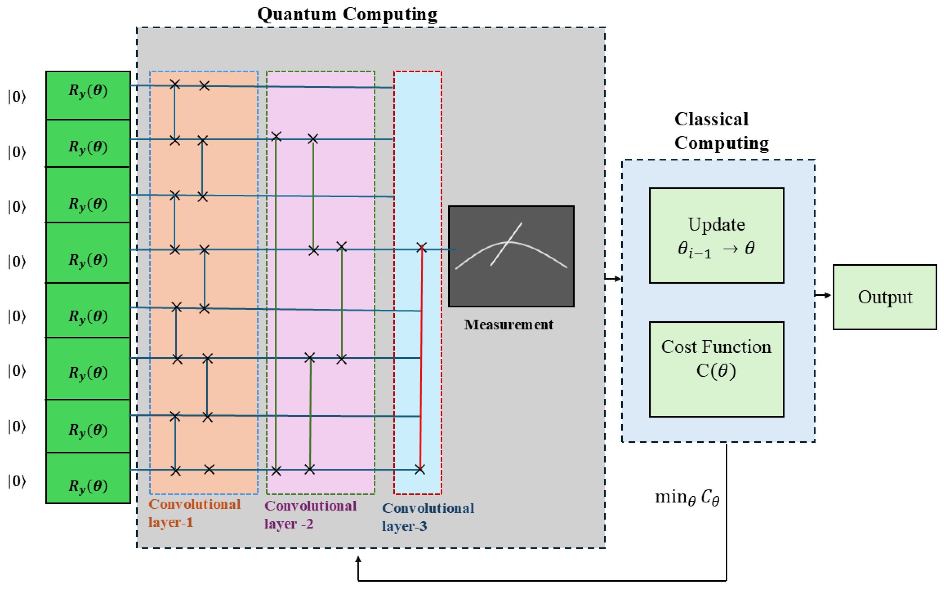
A crucial aspect of building a QCNN model is selecting an appropriate ansatz, because it determines how quantum operations are applied to extract and process features from quantum-encoded data. In classical CNNs, convolutional filters and pooling layers follow predefined mathematical operations to extract features from images. In contrast, QCNNs offer more flexibility by using customizable two-qubit unitary operations in both the convolutional and pooling steps. These quantum operations act like filters, identifying key patterns in the data while simultaneously reducing the size of the quantum system, similar to how pooling simplifies data in classical networks. This adaptability allows QCNNs to efficiently process quantum-encoded information while leveraging the advantages of quantum computing. The flexibility in choosing these unitary operations allows QCNN models to be tailored for different datasets and tasks. By optimizing the ansatz, researchers can improve the QCNN’s ability to acquire meaningful representations while keeping the necessary qubits and quantum gates as low as possible. A schematic of the QCNN used in this study is given in Figure 4.

1.

Encoding and Convolution Filter

In this model, angle encoding is used for state preparation (shown in Figure 4 in green colored box), where classical data are transformed into a quantum state using $R_y\left(\theta \right)$ rotations on 8 qubits. The Ry gate is used here because it applies rotations around the Y-axis of the Bloch sphere, which are easy to visualize and interpret. In variational quantum circuits, having a single rotation axis simplifies training and reduces the risk of overparameterization. Most quantum hardware and simulators like PennyLane natively support Ry gates with lower error rates than general U3 gates, making them a practical and reliable choice. Paired with CNOTs for entanglement, this structure supports efficient and interpretable quantum feature extraction while remaining scalable. This structure consists of three convolutional layers, each applying a quantum unitary operation $U_{SU}$ to specific pairs of qubits. The first convolution layer applies unitary operation to adjacent qubits. The second convolution layer applies gates to long-range qubits, which leads to an increase in connectivity. The third convolution layer reduces the information to single qubit and applies $U_{SU}$ to the initial qubit (Qubit 0) and the middle qubit (Qubit 4) to summarize extracted features. This is similar to the final fully connected layer in a classical CNN: it effectively merges information from different regions of the qubit, registering them into a single representation. QCNN ultimately measures a single qubit by computing the Pauli-Z expectation value of the middle qubit.

2.

Cost Function

The ansatz’s variational parameters are optimized to reduce the cost function based on the training dataset. In this research, we assess the performance of QCNN architecture using mean squared error loss function.

Mean Squared Error Loss Function

The output of our quantum circuit is not a probability in the traditional sense. It is an expectation value of a Pauli-Z observable, which ranges from −1 to +1. Since this output is continuous rather than probabilistic, MSE works naturally to measure how close the model’s output is to the target label (which we map accordingly).

To formulate the cost function for training the QCNN, first, the original data Labels 0 and 1 needs to be mapped to +1 and −1, respectively. This is performed because the Pauli-Z measurement of a qubit can only yield eigenvalues +1 or −1. Mathematically, this mapping is represented as

$$y_i^{\prime }=1-2y_i$$

(15)

where

$$y_i=0\Rightarrow y_i^{\prime }=1$$

$$y_i=1\Rightarrow y_i^{\prime }=-1$$

The MSE cost function between QCNN’s prediction and actual class label is shown in Equation (16):

$$C\left(\theta \right)={\displaystyle \frac{1}{N}}\sum _{i=1}^N{\left(O_z\left({\theta }_i\right)-y_i^{\prime }\right)}^2$$

(16)

$C\left(\theta \right)$ is the cost function that we want to minimize.

$O_z\left({\theta }_i\right)$ indicates the Pauli-Z expectation value of the output qubit for the $i^{\mathrm{th}}$ training example. This is the value predicted by the QCNN. The Pauli-Z expectation is given by $O_z=\langle \psi \left|Z\right|\psi \rangle =|a_i{|}^2-{\left|b_i\right|}^2$, where $a_i$ is the amplitude of the qubits to be measured in the state |0〉 and $b_i$ is the amplitude of the qubit to be measured in the state |1〉. As we mapped $y_i$ with $y_i^{\prime }$ in Equation (15), then we can say that if $a_i$ is large, the measurement is likely to be +1 (closer to state $|0\rangle )$ and if $b_i$ is large, the measurement is likely to be −1 (closer to state |1〉). By minimizing the cost function, QCNN adjusts its parameters such that, if the label is 0, the state should be as close as possible to |0〉, meaning $a_i$ is maximized. If the label is 1, the state should be as close as possible to |1〉, meaning $b_i$ is maximized.

3.

Training

To train this model, the Adam optimizer (Adaptive Moment Estimation) is employed with an initial learning rate of 0.01. A smaller value of learning rate results in slower but stable training and higher value can cause instability. To enhance training efficiency, we implement a learning rate scheduler and use early stopping in Keras to mitigate overfitting. Training is set to a maximum of 100 epochs. Instead of using all training data at once, the model selects 25 random samples per training step. This is known as minibatch training, which improves efficiency and convergence.

If the validation loss does not improve for three consecutive epochs, the learning rate is reduced by a factor of 0.1. The updated learning rate follows the equation

$$\mathrm{new}\mathrm{learning}\mathrm{rate}=0.1\times \mathrm{previous}\mathrm{learning}\mathrm{rate}$$

(17)

5.4. Computational Cost Analysis

In our QCNN, we use a total of 45 trainable parameters spread across three convolutional layers. Each layer applies a parameterized quantum unitary (U_SU4), which consists of a fixed set of rotation and entangling gates (mostly RY, RZ, U3, and CNOT gates). Across the full circuit, a single forward pass typically involves around 150 to 170 quantum gate operations. This is relatively lightweight compared to even a small classical CNN, which requires hundreds to thousands of parameters and significantly more floating-point operations (FLOPs) to process and backpropagate through layers of filters and feature maps.

In terms of memory, our model uses only 8 qubits and does not store intermediate data such as convolutional outputs, pooling layers, or dense activations, making it highly efficient in resource usage. Training was performed using the Adam optimizer, and the model reached stable accuracy within 100 iterations using batch sizes of 25, demonstrating low training overhead.

While direct comparisons of energy consumption between quantum and classical systems remain difficult due to hardware differences, it is worth noting that quantum gate operations are theoretically more energy-efficient than classical GPU operations. Additionally, by avoiding deep circuits and redundant layers, our QCNN remains computationally lean and suitable for near-term quantum hardware.

6. Performance Measures

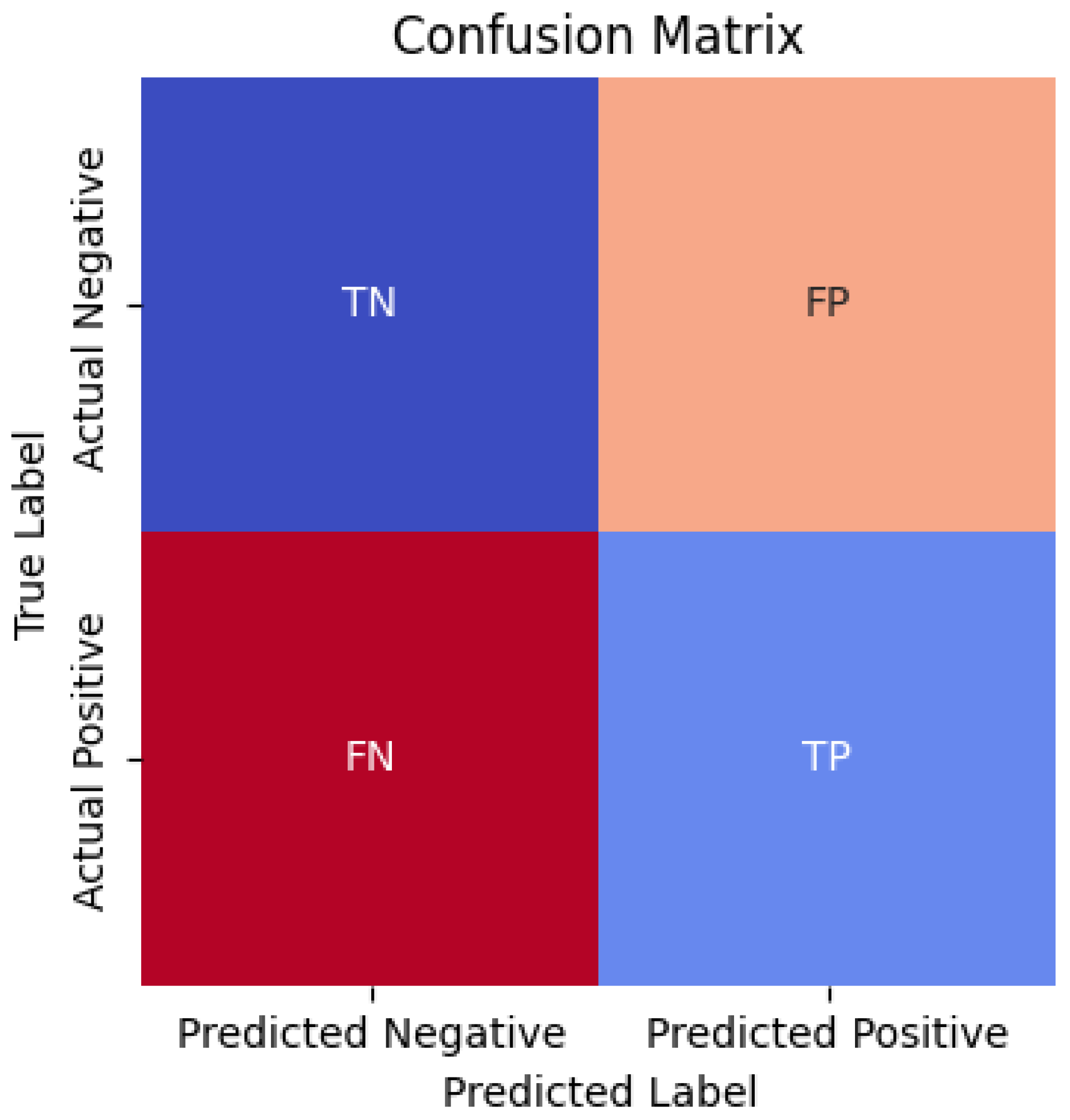
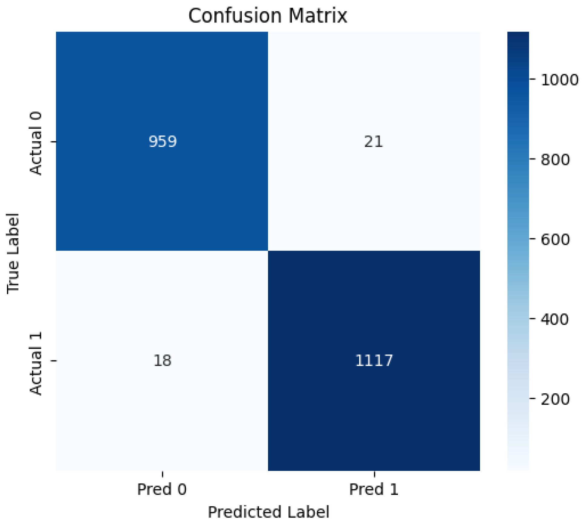
The effectiveness of the classification model is assessed using parameters such as accuracy, precision, recall, and F1 score. The confusion matrix for a two-class dataset is given in Figure 5.

Accuracy is described as the ratio of accurately classified instances compared to the overall count of instances.

$$\mathrm{Accuracy}={\displaystyle \frac{TP+TN}{TP+TN+FP+FN}}$$

Recall, also referred to as Sensitivity or True Positive Rate, quantifies the percentage of actual positive instances that are accurately identified.

$$\mathrm{Recall}={\displaystyle \frac{TP}{TP+FN}}$$

Precision indicates the percentage of predicted positive instances that are truly positive.

$$\mathrm{Precision}={\displaystyle \frac{TP}{TP+FP}}$$

The F1-score represents the harmonic average of precision and recall, offering a balanced measure when there is an uneven class distribution.

$$\mathrm{F}1=2\times {\displaystyle \frac{\mathrm{Precision}\times \mathrm{Recall}}{\mathrm{Precision}+\mathrm{Recall}}}={\displaystyle \frac{2\times TP}{2\times TP+FP+FN}}$$

7. Results and Discussion

1.

MNIST

This segment showcases the performance results of the QCNN framework in binary classification conducted using PennyLane. The image labels corresponding to digits 0 and 1 are selected, and each of these $28\times 28$ gray-scale images are resized to $8\times 1$. Since the focus is on 0 and 1, we take 12,665 training images and 2115 testing images out of 60,000 training and 10,000 testing images.

7.1. Performance

To assess the performance of our QCNN model, the epochs were set to 100 for both training and validation. To measure its effectiveness, accuracy and loss were calculated using a test set.

Figure 6 and Figure 7 illustrate how efficiency and loss evolved over the course of training.

The continuous decline in both training and validation losses indicates that the model was robust and successfully identified meaningful features in the data.

7.2. Accuracy and Loss

7.2.1. Accuracy Metrics

Figure 6 demonstrates that the trend of training, testing, and validation accuracy. Training accuracy rapidly increases between Epochs 10 and 30, showing strong learning progression. It approaches values above 90% at Epoch 30, where it stabilizes with minor fluctuations and remains consistently high near 98% in later epochs, demonstrating that the framework successfully captures the underlying patterns in the training data.

Validation accuracy (orange line with squares) initially starts at around 50%, similar to training accuracy and follows a similar increasing trend as training accuracy but with slightly more fluctuations. After Epoch 30, it stabilizes around 95–98%, maintaining consistency across later epochs. The difference between training and validation accuracy is minimal, suggesting that the framework generalizes well.

The final test accuracy is 97.26%, as represented by the horizontal red dashed line. After training for 100 epochs, when we evaluate the model on the held-out test set, our model correctly classifies about 97 out of every 100 test images. This is very close to the best validation and training accuracies. This demonstrates that the model maintains strong performance on unseen data, confirming its reliability.

7.2.2. Loss Metrics

As depicted in Figure 7, training loss starts high at 1.34 in the initial epochs and drops sharply within the first 20 epochs, indicating rapid learning. it continues to decrease gradually and stabilizes near 0.1–0.2 after 50 epochs. Small fluctuations are observed, but overall, it follows a downward trend and reaches at 0.0854 at last iteration, showing effective learning.

Similarly, validation loss dropped from 1.0480 to 0.1054, demonstrating that the framework effectively captured patterns from the training data while maintaining strong adaptability to unseen data.

Both losses converge at a low value, which means the model is not overfitting and successfully captures patterns in the data.

The final test loss is 0.1068. Since the test loss is close to the stabilized training and validation loss, this suggests the model has strong generalization capability.

7.3. Principal Component Analysis Visualization

Figure 8 represents a PCA visualization of the MNIST dataset, specifically comparing digits 0 and 1. The original MNIST images (28 × 28 pixels) are projected onto two principal components for visualization. This transformation reduces the complex data into a 2D plane, enhancing the visibility of underlying structures and separability between classes. Blue points represent digit 0 samples. Red points represent digit 1 samples. The two digits are clearly separated, showing that PCA effectively captures meaningful differences between them.

There is a noticeable overlapping region in the center, where red and blue dots mix. This suggests that some instances of digits 0 and 1 have similar characteristics, making them harder to separate using just two PCA components.

7.4. Confusion Matrix

The effectiveness of this classification framework is shown using a confusion matrix (shown in Figure 5), which compares actual and predicted classifications. It provides insights into True Positives (TPs), False Positives (FPs), True Negatives (TNs), and False Negatives (FNs). Confusion matrix generated for this model is given in Figure 9. Most values on the diagonal (top left to bottom right) interprets that the model makes very little error in the classification of 0 and 1.

For this binary classification task, the framework attains a precision of 98.2%, a recall of 98.4%, an F1-score of 98.3%, and a specificity of 97.9%. These high values indicate that the model effectively minimizes both false positives and false negatives. In general, a framework with strong accuracy, precision, recall, F1-score, and specificity is considered effective and well-performing.

2.

Wine Dataset

After successfully building and testing the QCNN model on the MNIST dataset, where it performed very well on binary digit classification, we wanted to see how it would handle a completely different type of data. So, we decided to extend the same model to the Wine dataset from the UCI Machine Learning Repository.

Unlike MNIST, which deals with image data, the Wine dataset is made up of chemical measurements from 178 wine samples, each belonging to one of three different cultivars. Since our quantum model uses 8 qubits, we selected the first 8 features from each sample to match the model’s input structure. The task was simplified to a binary classification problem: predicting whether a sample belongs to class 0 or not. We split the data into training, validation, and testing sets to make sure the model could generalize well to new, unseen data.

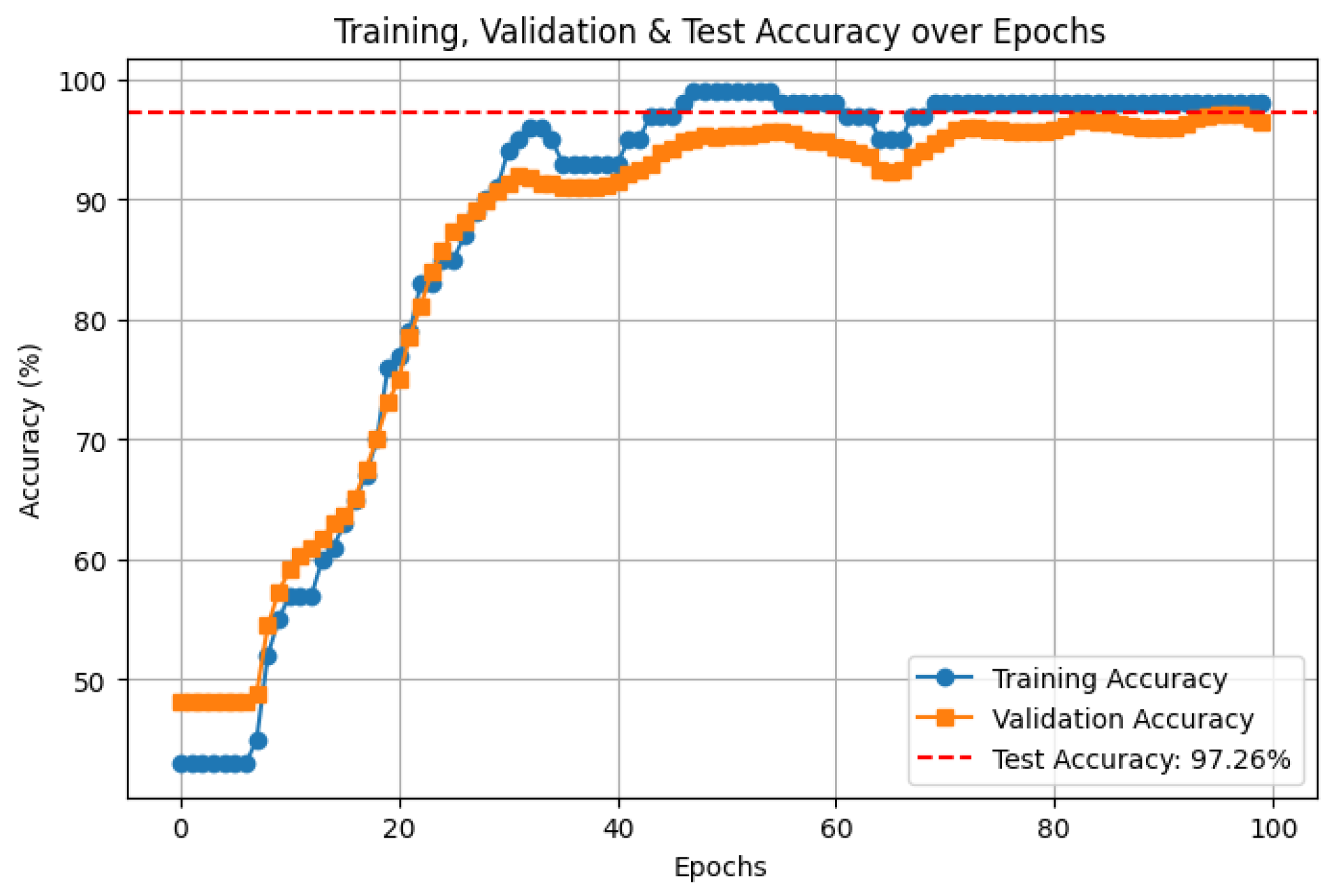
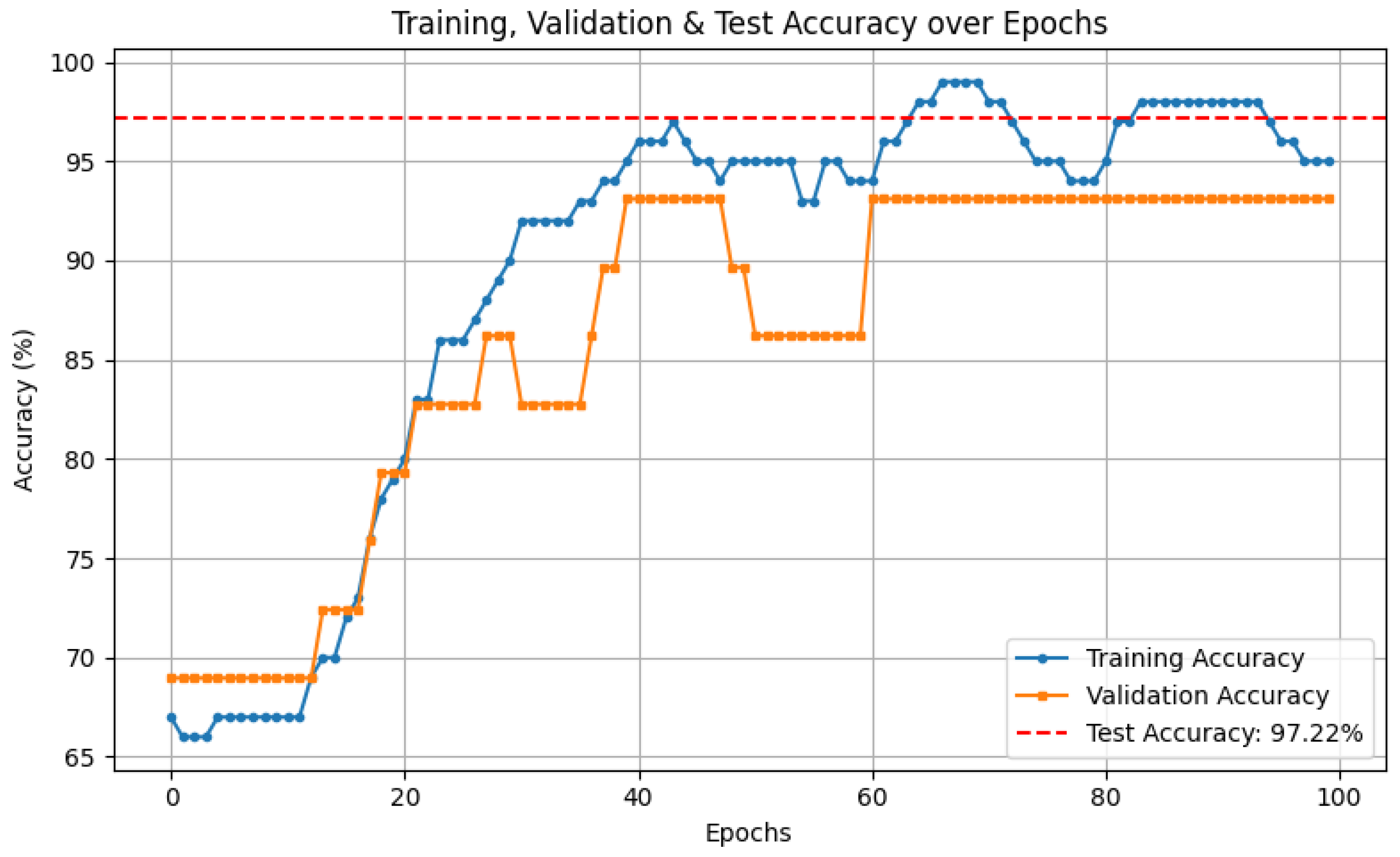
Figure 10 demonstrates the progression of training, validation, and test accuracy of the QCNN model over 100 epochs when applied to the Wine dataset. The training accuracy (blue line with circles) starts modestly around 66% but shows a rapid and steady rise between Epochs 10 and 40, indicating strong learning and effective pattern recognition. By Epoch 40, it crosses the 90% mark and continues to improve, stabilizing near 98% towards the later stages of training. This consistent high accuracy reflects the model’s strong ability to learn from the training data.

The validation accuracy (orange line with squares) begins around 68%, closely following the training curve. It rises steadily, though with slightly more fluctuations, especially between Epochs 30 and 60. These variations are natural and suggest the model is encountering slightly more variation in the validation data. Despite these ups and downs, the validation accuracy ultimately stabilizes around 93% in the later epochs, aligning well with the training curve. The close alignment of training and validation accuracies indicates that the model is not overfitting and generalizes well to unseen data.

The test accuracy, marked by the horizontal red dashed line, reaches a final value of 97.22%. This high performance on the test set confirms that the model has not only learned the training patterns effectively but also retained the ability to classify unseen data with impressive precision. The strong agreement between training, validation, and test accuracies demonstrates the robustness and reliability of the extended QCNN model on the Wine dataset.

8. Conclusions and Future Directions

This study presented a QCNN for the two-class classification, initially applied to the MNIST dataset, achieving a high 97.26% accuracy on the test set. The framework was assessed using key performance metrics such as precision, accuracy, recall, and F1-score, all of which remained consistently around 98%, demonstrating its strong classification capabilities. Additionally, the confusion matrix analysis showed well-balanced values for True Positives, True Negatives, False Positives, and False Negatives, indicating that the framework efficiently differentiates digit categories with minimal errors. Building on this success, the same QCNN architecture was extended to the Wine dataset, reframed as a binary classification problem (Class 0 vs. not Class 0). After adapting the input to match the available qubit resources, the model once again delivered high performance, reaching a 97.22% test accuracy. The training and validation accuracies closely followed each other throughout the training process, showing no signs of overfitting and confirming the model’s generalization strength. This consistent success across two structurally different datasets highlights the QCNN’s robustness, adaptability, and potential in handling diverse classification problems in Quantum Machine Learning.

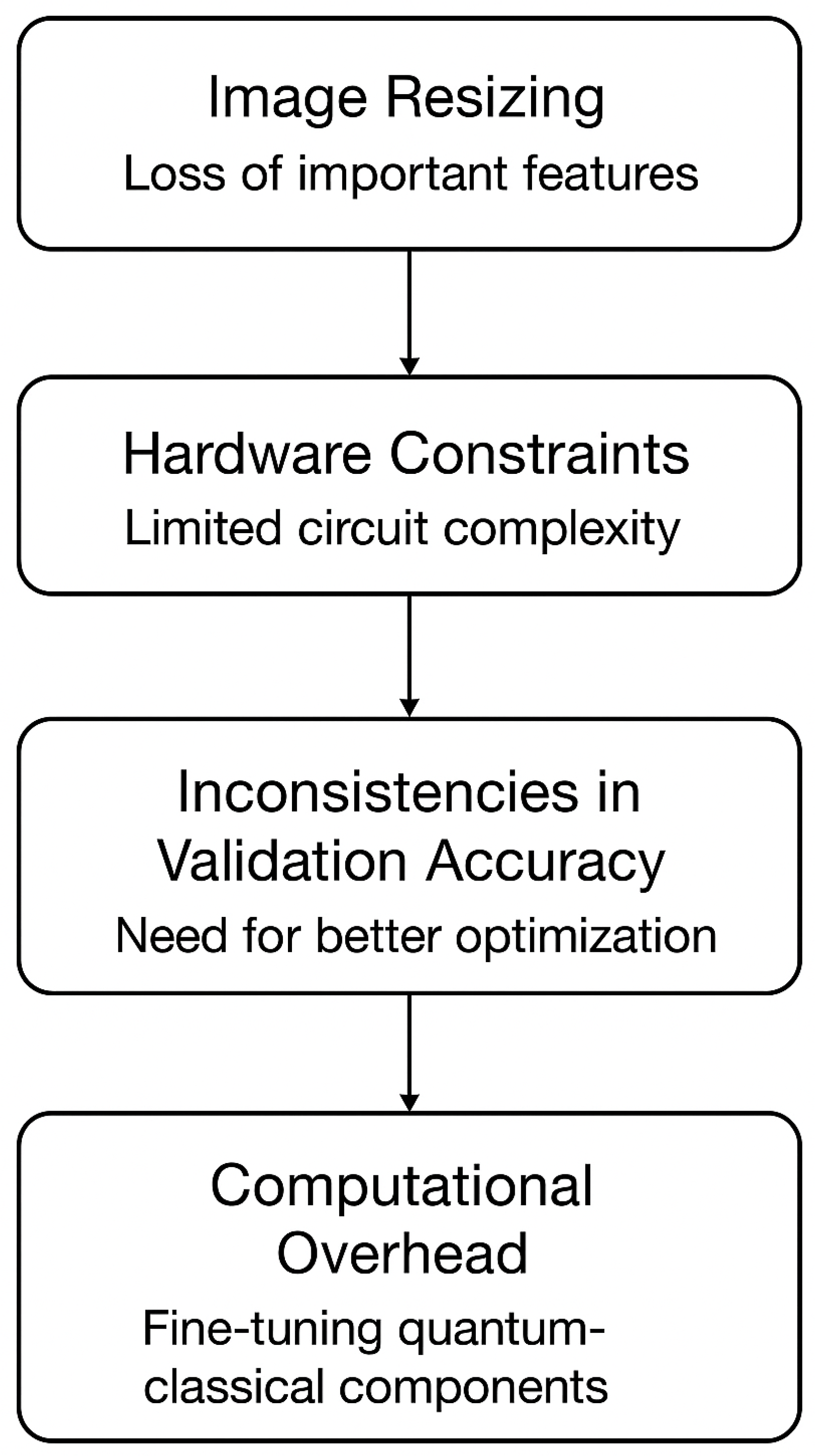
Despite its success, the study encountered a few challenges. One major issue was image resizing, as reducing the resolution sometimes led to the loss of important features, affecting classification accuracy. Hardware constraints also played a role, limiting the complexity of the quantum circuits and restricting the model’s scalability. Additionally, we observed inconsistencies in validation accuracy for the WINE dataset, highlighting the need for better optimization techniques to improve reliability. Another challenge was the computational overhead required to fine-tune the quantum and classical components, which increased processing time (some limitations occur in performing this study are depicted in the Figure 11). Overall, this study emphasized the promise of QCNNs in machine learning applications, including areas like medical imaging, pattern recognition, and automated decision-making systems. Moving forward, efforts should be directed toward improving data resolution techniques, refining quantum circuit designs, and overcoming hardware limitations to further enhance the effectiveness of QCNNs in real-world applications.

Future research on QCNNs should focus on both improving data handling and overcoming hardware challenges. On the data side, adaptive encoding strategies can be explored to avoid excessive image resizing, which often leads to the loss of important features. Techniques such as hybrid pre-processing with classical CNNs may help preserve critical visual information, while the development of quantum feature maps could further enhance the processing of high-dimensional data. At the same time, the limited number of qubits and inherent noise in current quantum devices constrain the depth and scalability of QCNNs. Addressing these issues requires the design of more hardware-efficient circuits and advanced error-mitigation methods. In addition, close collaboration with hardware developers could accelerate the creation of specialized quantum architectures optimized for machine learning applications, making QCNNs more practical and effective in real-world scenarios.

References

1. Alzubaidi, L.; Zhang, J.; Humaidi, A.J.; Al-Dujaili, A.; Duan, Y.; Al-Shamma, O.; Santamaría, J.; Fadhel, M.A.; Al-Amidie, M.; Farhan, L. Review of deep learning: Concepts, CNN architectures, challenges, applications, future directions. J. Big Data 2021, 8, 53. [Google Scholar] [CrossRef] [PubMed]
2. Zhou, L.; Cai, J.; Ding, S. The identification of ice floes and calculation of sea ice concentration based on a deep learning method. Remote Sens. 2023, 15, 2663. [Google Scholar] [CrossRef]
3. Cai, J.; Ding, S.; Zhang, Q.; Liu, R.; Zeng, D.; Zhou, L. Broken ice circumferential crack estimation via image techniques. Ocean Eng. 2022, 259, 111735. [Google Scholar] [CrossRef]
4. Xia, W.; Pu, L.; Zou, X.; Shilane, P.; Li, S.; Zhang, H.; Wang, X. The design of fast and lightweight resemblance detection for efficient post-deduplication delta compression. Acm Trans. Storage 2023, 19, 1–30. [Google Scholar] [CrossRef]
5. Li, M.; Jia, T.; Wang, H.; Ma, B.; Lu, H.; Lin, S.; Cai, D.; Chen, D. Ao-detr: Anti-overlapping detr for X-ray prohibited items detection. IEEE Trans. Neural Netw. Learn. Syst. 2024, 36, 12076–12090. [Google Scholar] [CrossRef]
6. Zhou, Z.; Li, Z.; Zhou, W.; Chi, N.; Zhang, J.; Dai, Q. Resource-saving and high-robustness image sensing based on binary optical computing. Laser Photonics Rev. 2025, 19, 2400936. [Google Scholar] [CrossRef]
7. Goodfellow, I.; Bengio, Y.; Courville, A.; Bengio, Y. Deep Learning Cambridge; MIT Press: Cambridge, MA, USA, 2016; Available online: http://www.deeplearningbook.org (accessed on 23 September 2025).
8. Wang, W.; Yin, B.; Li, L.; Li, L.; Liu, H. A Low Light Image Enhancement Method Based on Dehazing Physical Model. Comput. Model. Eng. Sci. (CMES) 2025, 143, 1595. [Google Scholar] [CrossRef]
9. Gan, X. GraphService: Topology-aware constructor for large-scale graph applications. ACM Trans. Archit. Code Optim. 2025, 22, 1–24. [Google Scholar] [CrossRef]
10. Gan, X.; Li, T.; Gong, C.; Li, D.; Dong, D.; Liu, J.; Lu, K. GraphCSR: A Degree-Equalized CSR Format for Large-scale Graph Processing. Proc. VLDB Endow. 2025, 18, 4255–4268. [Google Scholar] [CrossRef]
11. Liu, J.; Jiang, G.; Chu, C.; Li, Y.; Wang, Z.; Hu, S. A formal model for multiagent Q-learning on graphs. Sci. China Inf. Sci. 2025, 68, 192206. [Google Scholar] [CrossRef]
12. Shi, J.; Liu, C.; Liu, J. Hypergraph-based model for modelling multi-agent q-learning dynamics in public goods games. IEEE Trans. Netw. Sci. Eng. 2024, 11, 6169–6179. [Google Scholar] [CrossRef]
13. Zhang, Z.W.; Liu, Z.G.; Martin, A.; Zhou, K. BSC: Belief shift clustering. IEEE Trans. Syst. Man Cybern. Syst. 2022, 53, 1748–1760. [Google Scholar] [CrossRef]
14. Yuan, X.; Sun, J.; Liu, J.; Zhao, Q.; Zhou, Y. Quantum simulation with hybrid tensor networks. Phys. Rev. Lett. 2021, 127, 040501. [Google Scholar] [CrossRef] [PubMed]
15. Zuo, C.; Zhang, X.; Zhao, G.; Yan, L. PCR: A parallel convolution residual network for traffic flow prediction. IEEE Trans. Emerg. Top. Comput. Intell. 2025, 9, 3072–3083. [Google Scholar] [CrossRef]
16. Zhu, J.; Wang, X.; Cao, G.; Xu, L.; Cao, Y. Quantum Interval Neural Network for Uncertain Structural Static Analysis. Int. J. Mech. Sci. 2025, 303, 110646. [Google Scholar] [CrossRef]
17. Ruan, Y.; Xue, X.; Shen, Y. Quantum image processing: Opportunities and challenges. Math. Probl. Eng. 2021, 2021, 6671613. [Google Scholar] [CrossRef]
18. Xu, L.; Wang, X.; Wang, Z.; Cao, G. Hybrid quantum genetic algorithm for structural damage identification. Comput. Methods Appl. Mech. Eng. 2025, 438, 117866. [Google Scholar] [CrossRef]
19. Wei, S.; Chen, Y.; Zhou, Z.; Long, G. A quantum convolutional neural network on NISQ devices. AAPPS Bull. 2022, 32, 2. [Google Scholar] [CrossRef]
20. Zuo, Y.; Hu, Y.; Xu, Y.; Wang, Z.; Fang, Y.; Yan, J.; Jiang, W.; Peng, Y.; Huang, Y. Learning Guided Implicit Depth Function with Scale-aware Feature Fusion. IEEE Trans. Image Process. 2025, 34, 3309–3322. [Google Scholar] [CrossRef]
21. Asif, H.; Basit, A.; Innan, N.; Kashif, M.; Marchisio, A.; Shafique, M. PennyLang: Pioneering LLM-Based Quantum Code Generation with a Novel PennyLane-Centric Dataset. arXiv 2025, arXiv:2503.02497. [Google Scholar]
22. Henderson, M.; Shakya, S.; Pradhan, S.; Cook, T. Quanvolutional neural networks: Powering image recognition with quantum circuits. Quantum Mach. Intell. 2020, 2, 2. [Google Scholar] [CrossRef]
23. Yousif, M.; Al-Khateeb, B.; Garcia-Zapirain, B. A new quantum circuits of quantum convolutional neural network for X-ray images classification. IEEE Access 2024, 12, 65660–65671. [Google Scholar] [CrossRef]
24. Reka, S.S.; Karthikeyan, H.L.; Shakil, A.J.; Venugopal, P.; Muniraj, M. Exploring quantum machine learning for enhanced skin lesion classification: A comparative study of implementation methods. IEEE Access 2024, 12, 104568–104584. [Google Scholar] [CrossRef]
25. Shi, S.; Wang, Z.; Li, J.; Li, Y.; Shang, R.; Zhong, G.; Gu, Y. Quantum convolutional neural networks for multiclass image classification. Quantum Inf. Process. 2024, 23, 189. [Google Scholar] [CrossRef]
26. Tomar, M.; Prajapat, S.; Kumar, D.; Kumar, P.; Kumar, R.; Vasilakos, A.V. Exploring the Role of Material Science in Advancing Quantum Machine Learning: A Scientometric Study. Mathematics 2025, 13, 958. [Google Scholar] [CrossRef]
27. Fukushima, K. Neocognitron: A self-organizing neural network model for a mechanism of pattern recognition unaffected by shift in position. Biol. Cybern. 1980, 36, 193–202. [Google Scholar] [CrossRef]
28. LeCun, Y.; Boser, B.; Denker, J.S.; Henderson, D.; Howard, R.E.; Hubbard, W.; Jackel, L.D. Backpropagation applied to handwritten zip code recognition. Neural Comput. 1989, 1, 541–551. [Google Scholar] [CrossRef]
29. LeCun, Y.; Bottou, L.; Bengio, Y.; Haffner, P. Gradient-based learning applied to document recognition. Proc. IEEE 1998, 86, 2278–2324. [Google Scholar] [CrossRef]
30. Hinton, G.E.; Srivastava, N.; Krizhevsky, A.; Sutskever, I.; Salakhutdinov, R.R. Improving neural networks by preventing co-adaptation of feature detectors. arXiv 2012, arXiv:1207.0580. [Google Scholar] [CrossRef]
31. Simonyan, K.; Zisserman, A. Very deep convolutional networks for large-scale image recognition. arXiv 2014, arXiv:1409.1556. [Google Scholar]
32. Szegedy, C.; Liu, W.; Jia, Y.; Sermanet, P.; Reed, S.; Anguelov, D.; Erhan, D.; Vanhoucke, V.; Rabinovich, A. Going deeper with convolutions. In Proceedings of the IEEE Conference on Computer Vision and Pattern Recognition, Boston, MA, USA, 7–12 June 2015; pp. 1–9. [Google Scholar]
33. He, K.; Zhang, X.; Ren, S.; Sun, J. Deep residual learning for image recognition. In Proceedings of the IEEE Conference on Computer Vision and Pattern Recognition, Las Vegas, NV, USA, 27–30 June 2016; pp. 770–778. [Google Scholar]
34. Huang, G.; Liu, Z.; Van Der Maaten, L.; Weinberger, K.Q. Densely connected convolutional networks. In Proceedings of the IEEE Conference on Computer Vision and Pattern Recognition, Honolulu, HI, USA, 21–26 July 2017; pp. 4700–4708. [Google Scholar]
35. Yang, Y.; Hospedales, T.M. Deep neural networks for sketch recognition. arXiv 2015, arXiv:1501.07873. [Google Scholar]
36. Ballester, P.; Araujo, R. On the performance of GoogLeNet and AlexNet applied to sketches. In Proceedings of the AAAI Conference on Artificial Intelligence, Phoenix, AZ, USA, 12–17 February 2016; Volume 30. [Google Scholar]
37. Karpathy, A.; Toderici, G.; Shetty, S.; Leung, T.; Sukthankar, R.; Li, F.-F. Large-scale video classification with convolutional neural networks. In Proceedings of the IEEE Conference on Computer Vision and Pattern Recognition, Columbus, OH, USA, 23–28 June 2014; pp. 1725–1732. [Google Scholar]
38. Sharma, N.; Jain, V.; Mishra, A. An analysis of convolutional neural networks for image classification. Procedia Comput. Sci. 2018, 132, 377–384. [Google Scholar] [CrossRef]
39. Jmour, N.; Zayen, S.; Abdelkrim, A. Convolutional neural networks for image classification. In Proceedings of the 2018 International Conference on Advanced Systems and Electric Technologies (IC_ASET), Hammamet, Tunisia, 22–25 March 2018; pp. 397–402. [Google Scholar]
40. Beohar, D.; Rasool, A. Handwritten digit recognition of MNIST dataset using deep learning state-of-the-art artificial neural network (ANN) and convolutional neural network (CNN). In Proceedings of the 2021 International Conference on Emerging Smart Computing and Informatics (ESCI), Pune, India, 5–7 March 2021; pp. 542–548. [Google Scholar]
41. Rebentrost, P.; Mohseni, M.; Lloyd, S. Quantum support vector machine for big data classification. Phys. Rev. Lett. 2014, 113, 130503. [Google Scholar] [CrossRef] [PubMed]
42. Ostaszewski, M.; Sadowski, P.; Gawron, P. Quantum image classification using principal component analysis. arXiv 2015, arXiv:1504.00580. [Google Scholar] [CrossRef]
43. Ruan, Y.; Xue, X.; Liu, H.; Tan, J.; Li, X. Quantum algorithm for k-nearest neighbors classification based on the metric of hamming distance. Int. J. Theor. Phys. 2017, 56, 3496–3507. [Google Scholar] [CrossRef]
44. Cong, I.; Choi, S.; Lukin, M.D. Quantum convolutional neural networks. Nat. Phys. 2019, 15, 1273–1278. [Google Scholar] [CrossRef]
45. Kerenidis, I.; Landman, J.; Prakash, A. Quantum algorithms for deep convolutional neural networks. arXiv 2019, arXiv:1911.01117. [Google Scholar] [CrossRef]
46. Li, Y.; Zhou, R.G.; Xu, R.; Luo, J.; Hu, W. A quantum deep convolutional neural network for image recognition. Quantum Sci. Technol. 2020, 5, 044003. [Google Scholar] [CrossRef]
47. Hur, T.; Kim, L.; Park, D.K. Quantum convolutional neural network for classical data classification. Quantum Mach. Intell. 2022, 4, 3. [Google Scholar] [CrossRef]
48. Yousif, M.; Al-Khateeb, B. Quantum Convolutional Neural Network for Image Classification. Fusion Pract. Appl. 2024, 15, 655–667. [Google Scholar]
49. Hassan, E.; Hossain, M.S.; Saber, A.; Elmougy, S.; Ghoneim, A.; Muhammad, G. A quantum convolutional network and ResNet (50)-based classification architecture for the MNIST medical dataset. Biomed. Signal Process. Control 2024, 87, 105560. [Google Scholar] [CrossRef]
50. Sayed, R.; Azmi, H.; Shawkey, H.; Khalil, A.H.; Refky, M. A systematic literature review on binary neural networks. IEEE Access 2023, 11, 27546–27578. [Google Scholar] [CrossRef]
51. Yao, P.; Wu, H.; Gao, B.; Tang, J.; Zhang, Q.; Zhang, W.; Yang, J.J.; Qian, H. Fully hardware-implemented memristor convolutional neural network. Nature 2020, 577, 641–646. [Google Scholar] [CrossRef] [PubMed]
52. Van Pham, K.; Van Nguyen, T.; Tran, S.B.; Nam, H.; Lee, M.J.; Choi, B.J.; Truong, S.N.; Min, K. Memristor binarized neural networks. J. Semicond. Technol. Sci. 2018, 18, 568–588. [Google Scholar] [CrossRef]
53. Pham, K.V.; Tran, S.B.; Nguyen, T.V.; Min, K.S. Asymmetrical training scheme of binary-memristor-crossbar-based neural networks for energy-efficient edge-computing nanoscale systems. Micromachines 2019, 10, 141. [Google Scholar] [CrossRef] [PubMed]
54. Huang, M.; Zhao, G.; Wang, X.; Zhang, W.; Coquet, P.; Tay, B.K.; Zhong, G.; Li, J. Global-gate controlled one-transistor one-digital-memristor structure for low-bit neural network. IEEE Electron Device Lett. 2020, 42, 106–109. [Google Scholar] [CrossRef]
55. Wu, H. CNN-Based Recognition of Handwritten Digits in MNIST Database. Research School of Computer Science, The Australia National University, Canberra, Australia. 2018. Available online: https://users.cecs.anu.edu.au/~Tom.Gedeon/conf/ABCs2018/paper/ABCs2018_paper_104.pdf (accessed on 23 September 2025).
56. Cohen, G.; Afshar, S.; Tapson, J.; Van Schaik, A. EMNIST: Extending MNIST to handwritten letters. In Proceedings of the 2017 International Joint Conference on Neural Networks (IJCNN), Anchorage, AK, USA, 14–19 May 2017; pp. 2921–2926. [Google Scholar]
57. Gope, B.; Pande, S.; Karale, N.; Dharmale, S.; Umekar, P. Handwritten digits identification using mnist database via machine learning models. IOP Conf. Ser. Mater. Sci. Eng. 2021, 1022, 012108. [Google Scholar] [CrossRef]
58. Qian, Y.; Wang, X.; Du, Y.; Wu, X.; Tao, D. The dilemma of quantum neural networks. IEEE Trans. Neural Netw. Learn. Syst. 2022, 35, 5603–5615. [Google Scholar] [CrossRef]
59. Nielsen, M.A.; Chuang, I.L. Quantum Computation and Quantum Information; Cambridge University Press: Cambridge, UK, 2010. [Google Scholar]
60. Oh, S.; Choi, J.; Kim, J. A tutorial on quantum convolutional neural networks (QCNN). In Proceedings of the 2020 International Conference on Information and Communication Technology Convergence (ICTC), Jeju Island, Republic of Korea, 16–18 October 2020; pp. 236–239. [Google Scholar]
61. Choi, J.; Oh, S.; Kim, J. Quantum approximation for wireless scheduling. Appl. Sci. 2020, 10, 7116. [Google Scholar] [CrossRef]
62. Abdulrida, R.; A-Monem, M.E.; Jaber, A.M. Quantum image watermarking based on wavelet and geometric transformation. Iraqi J. Sci. 2020, 61, 153–163. [Google Scholar] [CrossRef]
63. Khan, A.A.; Ahmad, A.; Waseem, M.; Liang, P.; Fahmideh, M.; Mikkonen, T.; Abrahamsson, P. Software architecture for quantum computing systems-A systematic review. J. Syst. Softw. 2023, 201, 111682. [Google Scholar] [CrossRef]
64. Kwak, Y.; Yun, W.J.; Jung, S.; Kim, J. Quantum neural networks: Concepts, applications, and challenges. In Proceedings of the 2021 Twelfth International Conference on Ubiquitous and Future Networks (ICUFN), Jeju Island, Republic of Korea, 17–20 August 2021; pp. 413–416. [Google Scholar]
65. Fisher, M.P.; Khemani, V.; Nahum, A.; Vijay, S. Random quantum circuits. Annu. Rev. Condens. Matter Phys. 2023, 14, 335–379. [Google Scholar] [CrossRef]
66. Zheng, J.; Gao, Q.; Lü, J.; Ogorzałek, M.; Pan, Y.; Lü, Y. Design of a quantum convolutional neural network on quantum circuits. J. Frankl. Inst. 2023, 360, 13761–13777. [Google Scholar] [CrossRef]
67. Huang, R.; Tan, X.; Xu, Q. Learning to learn variational quantum algorithm. IEEE Trans. Neural Netw. Learn. Syst. 2022, 34, 8430–8440. [Google Scholar] [CrossRef] [PubMed]
68. LaRose, R.; Coyle, B. Robust data encodings for quantum classifiers. Phys. Rev. A 2020, 102, 032420. [Google Scholar] [CrossRef]
69. Kosaraju, N.; Sankepally, S.R.; Mallikharjuna Rao, K. Categorical data: Need, encoding, selection of encoding method and its emergence in machine learning models-A practical review study on heart disease prediction dataset using pearson correlation. In Proceedings of the International Conference on Data Science and Applications: ICDSA 2022, Kolkata, India, 26–27 March 2022; Volume 1, pp. 369–382. [Google Scholar]
70. Yao, F.; Zhang, H.; Gong, Y. Difsg2-ccl: Image reconstruction based on special optical properties of water body. IEEE Photonics Technol. Lett. 2024, 36, 1417–1420. [Google Scholar] [CrossRef]
71. Hu, C.; Dong, B.; Shao, H.; Zhang, J.; Wang, Y. Toward purifying defect feature for multilabel sewer defect classification. IEEE Trans. Instrum. Meas. 2023, 72, 1–11. [Google Scholar] [CrossRef]
Figure 1. Framework for a CNN model.
Mathematics 13 03148 g001
Figure 2. General framework of a QCNN model.
Mathematics 13 03148 g002
Figure 3. MNIST dataset images (a,b).
Mathematics 13 03148 g003
Figure 4. Schematic diagram of the QCNN algorithm used in this study.
Mathematics 13 03148 g004
Figure 5. Confusion matrix.
Mathematics 13 03148 g005
Figure 6. Accuracy vs. epochs.
Mathematics 13 03148 g006
Figure 7. Loss VS. epochs.
Mathematics 13 03148 g007
Figure 8. PCA visualization of 0 and 1.
Mathematics 13 03148 g008
Figure 9. Confusion matrix for the model.
Mathematics 13 03148 g009
Figure 10. Accuracy vs. epochs.
Mathematics 13 03148 g010
Figure 11. Limitations encountered in this study.
Mathematics 13 03148 g011