Abstract
This paper investigates the teleparallel Robertson–Walker (TRW) gravity solutions for a Chaplygin gas, and then for any polytropic gas cosmological source. We use the TRW gravity field equations (FEs) for each k-parameter value case and the relevant gas equation of state (EoS) to find the new teleparallel solutions. For flat cosmological case, we find analytical solutions valid for any cosmological scale factor. For curved cosmological cases, we find new approximated teleparallel solutions for slow, linear, fast and very fast universe expansion cases summarizing by a double power-law function. All the new solutions will be relevant for future cosmological applications on dark matter, dark energy (DE) quintessence, phantom energy, Anti-deSitter (AdS) spacetimes and several other cosmological processes.
Keywords:
Teleparallel Robertson-Walker; Chaplygin gas; polytropic gas; teleparallel F(T)-type solution; Polytropic and Chaplygin Conservation Laws; cosmological spacetimes; cosmological teleparallel solutions MSC:
83D05
1. Introduction
The teleparallel gravity is a frame-based and alternative theory to general relativity (GR) fundamentally defined in terms of the coframe and the spin-connection [1,2,3,4,5,6,7]. These two last quantities define the torsion tensor and torsion scalar T. We remind that GR is defined by the metric and the spacetime curvatures , and R. Under some considerations, we can determine the symmetries for any independent coframe/spin-connection pairs, and then spacetime curvature and torsion are defined as geometric objects [4,5,6,7,8,9]. Any geometry described by a such pair whose curvature and non-metricity are both zero ( and conditions) is a teleparallel gauge-invariant geometry (valid for any ). The fundamental pairs must satisfy two Lie derivative-based relations and we use the Cartan–Karlhede algorithm to solve these two fundamental equations for any teleparallel geometry. For a pure teleparallel gravity spin-connection solution, we also solve the null Riemann curvature condition leading to a Lorentz transformation-based definition of the spin-connection . There is a direct equivalent to GR in teleparallel gravity: the teleparallel equivalent to GR (TEGR) which generalizes to teleparallel -type gravity [7,9,10,11,12]. All the previous considerations are also adapted for the new general relativity (NGR) (refs. [13,14,15] and refs. therein), the symmetric teleparallel -type gravity (refs. [16,17,18,19] and refs. therein) and some extended theories like -type, -type, -type, and several other ones (refs. [20,21,22,23,24,25,26,27,28,29] and refs. therein). In the current paper we will restrict our study to the teleparallel gravity framework.
There is a large number of research papers on spherically symmetric spacetimes and solutions in teleparallel gravity using a large number of approaches, energy-momentum sources and made for various purposes [30,31,32,33,34,35,36,37,38,39,40,41,42,43,44,45,46,47,48,49,50,51,52,53,54,55,56]. But there is a special class of teleparallel spacetime in which the field equations (FEs) are purely symmetric: the teleparallel Robertson–Walker (TRW) spacetime [55,56,57]. This type of spacetime is defined in terms of the k-parameter where is a flat cosmological spacetime, cases are, respectively, positive and negative space cosmological curvature [58,59,60,61]. We have proven that a such teleparallel geometry is described by a Lie algebra group, where the fourth to sixth Killing Vectors (KVs) are characteristic of this spacetime [56,57]. The main apparent consequence of additional KVs is the trivial antisymmetric parts of FEs. The same spacetime geometry structure also exists for some extensions such as teleparallel gravity [62,63,64,65,66]. We have found teleparallel and solutions for perfect fluid (PF) and scalar field (SF) sources. In the last case, the teleparallel and solutions are scalar potential-independent and only SF-dependent [55,62]. But there are additional possible sources of energy-momentum which can lead to new further teleparallel solutions in -type, but also for extensions.
The dark energy (DE) states are usually studied by using the PF equivalent equation of state (EoS) , where is the DE index (or quintessence index in some refs.) [67,68,69]. The possible DE forms in terms of are as follows:
- Quintessence : This describes a controlled accelerating universe expansion where energy conditions are always satisfied, i.e., [70,71,72,73,74,75,76,77,78,79,80,81,82]. This usual DE form has been significantly studied in the literature in recent decades for the fascination it provokes and the realism of the models.
- Phantom energy : This describes an uncontrolled universe expansion accelerating toward a Big Rip event (or singularity) [83,84,85,86,87,88,89,90,91]. The energy condition is violated, i.e., . But this DE form is fascinating because we can find new teleparallel solutions and physical models.
- Cosmological constant : This is an intermediate limit between the quintessence and phantom DE states, where . A constant SF source added by a positive scalar potential will directly lead to this primary DE state. Note that a negative scalar potential (i.e., ) will not lead to a positive cosmological constant and/or a DE solution.
- Quintom models: This is a mixture of previous DE types, usually described by double SF models [92,93,94,95,96,97]. This type of model is more complex to study and solve in general. Several types of models are in principle possible, and these physical processes need further studies in the future.
There are, in the recent literature on teleparallel gravity and its extension, a number of papers discussing possible solutions in static, radial-dependent, time-dependent and cosmological teleparallel models [48,49,50,51,52,55,56,62,98,99,100]. Most of those are suitable for DE models, in particular for quintessence DE state. We use cosmological PF as SF approaches, and we find that the solution classes are similar in the both cases. Some of these papers aimed to test some simple teleparallel solutions, such as power-law and the polynomial solution, on the cosmological models such as the well-known Lambda Cold Dark Matter (CDM) model limits [98,99,100]. Therefore, we also need to test some non-linear PF-based universe models and determine the non-linearity level of a typical cosmological PF-based universe.
The quartessence model is a unified model of DE and Dark Matter (DM) arising from a Chaplygin cosmological gas. The DE and DM are two states of a single and simple quartessence dark cosmological fluid [101,102,103,104,105]. This non-linear cosmological fluid model can be considered as an alternative and unified explanation of DE and DM evolving in the universe and influencing the cosmological processes. For polytropic gases, there are additional possible physical models arising from this class of EoS-based cosmological solutions [106,107,108,109,110,111,112,113]. But the Chaplygin, polytropic gas and any superposition of those models in general can explain not only DE and DM mixed or separate models, but also any non-linear cosmological gas and fluid system at the limit [114]. Most of the previous works have been done in the GR (or -type) framework, but these last cases may also arise in teleparallel theories of gravity. Under this last consideration, the current investigation concerning the Chaplygin and polytropic fluids deserves to be achieved in teleparallel framework and constitutes the main aim of the paper, in particular for the -type case. Ultimately, we want to build a pure teleparallel quartessence and polytropic-based cosmology, allowing us to study more realistic universe models.
Ultimately we want to study in detail the quartessence suitable teleparallel cosmological solutions and its physical impacts. Therefore we need, at the current stage, to find the possible Chaplygin and polytropic cosmological gas teleparallel gravity solutions in a Robertson–Walker spacetime (TRW). We had found the TRW geometry and we had solved the TRW FEs and conservation laws (CL) for PF and SF solutions in teleparallel and gravities [55,56,57,62]. But we can go further and aim to solve for polytropic and Chaplygin cosmological gases teleparallel solutions as the next step. To satisfy this aim, we will use the same TRW geometry, FEs and CLs to develop the teleparallel Chaplygin solutions in Section 3 and the teleparallel polytropic solutions in Section 4. We will then compare and highlight the similarities and differences by using graphs and propose future experimental data-based analysis guidelines in Section 5 before concluding the current paper in Section 6.
2. Summary of Teleparallel Gravity and Field Equations
2.1. Teleparallel -Gravity Theory Field Equations and Torsional Quantities
The teleparallel -type gravity action integral with any gravitational source is [2,3,5,7,47,48,49,50,51,52,55]:
where h is the coframe determinant, is the coupling constant and is the gravitational source term. We will apply the least-action principle on Equation (1) to find the symmetric and antisymmetric parts of FEs as [47,48,49,50,51,52,55]:
with the Einstein tensor, the energy-momentum, the gauge metric and the coupling constant. The torsion tensor , the torsion scalar T and the super-potential are defined as [5]
Equation (4) can be expressed in terms of the three irreducible parts of torsion tensor as
where,
We usually solve in teleparallel gravity, Equations (2) and (3). Therefore in refs. [55,56,57], we showed that Equation (3) is trivially satisfied despite a non-zero spin-connection, because the teleparallel geometry is purely symmetric. Only Equation (2) is non-trivial and will be explicitly solved in detail.
2.2. Teleparallel Robertson–Walker Spacetime Geometry
Any frame-based geometry in teleparallel gravity on a frame bundle is defined by a coframe/spin-connection pair and a field . The geometry must satisfy the fundamental Lie derivative-based equations [5,6,55,56,57]:
where is the spin-connection in terms of the differential coframe and is the linear isotropy group component. In addition for a pure teleparallel -type gravity, we must also satisfy the null Riemann curvature condition . For TRW spacetime geometries on an orthonormal frame, the coframe/spin-connection pair and solutions are [55,56,57]
where and are depending on k-parameter and defined by
- : ,
- : and ,
- : and .
For any and , we will obtain the same symmetric FEs set to solve for each subcases depending on k-parameter. The previous coframe/spin-connection pair was found by solving Equation (9) and condition as defined in ref. [5]. These solutions were also used in TRW spacetime recent works [55,56,57]. The TRW spacetime structure is typically explanable by a Lie algebra group. The FEs to be solved in the current paper are defined for each k-parameter cases and will lead to additional new teleparallel solution classes. The FEs defined by Equations (2) and (3) are still purely symmetric and valid on proper frames, as showed in refs. [55,56,57]. Equation (3) are trivially satisfied, and we will solve Equation (2) for each k-parameter case.
2.3. Conservation Laws and Field Equations of Cosmological Perfect Fluids
The canonical energy-momentum and its GR CLs are obtained from term of Equation (1) as [3,7]
where the covariant derivative and the conserved energy-momentum tensor. The antisymmetric and symmetric parts of are [47,48,49,50,51,52,55]
where is the symmetric part of . Equation (12) also imposes the symmetry of and Equation (13) the condition. Equation (13) is valid only when the matter field interacts with the metric defined from the coframe and the gauge , and is not directly coupled to the gravity. This consideration is only valid for the null hypermomentum case (i.e., ) as discussed in refs. [48,49,50,51,52,54,55]. This last condition on hypermomentum is defined from Equations (2) and (3) as [54]
There are more general teleparallel definitions and CLs, but this does not really concern the teleparallel -gravity situation [54,115,116,117].
For a TRW spacetime geometry defined by Equations (10) and (11), Equation (12) for a fluid is [55,56,57]
where is the Hubble parameter. The general FEs system for TRW cosmological spacetimes are [55,56,57]
- flat or non-curved:The pure vacuum solution ( and ) to Equations (19) and (20) is . However for any , we can set as cosmological scale and as solution ansatz, and we find the unified FE by merging Equations (19) and (20):Equation (21) is the general unified FE to solve for any EoS and CL. This is easy to solve, and the solution will be an easy-to-compute integral equation.
- negative curved:From Equation (24) and using ansatz, we find a characteristic equation yielding to solutions:The possible solutions of Equation (25) are
- (a)
- (slow expansion):
- (b)
- (linear expansion):
- (c)
- (fast expansion):
- (d)
- (very fast expansion limit):
- positive curved:From Equation (35) and using ansatz, we find the characteristic equation for :The possible solutions of Equation (36) are
- (a)
- (slow expansion):
- (b)
- (linear expansion):
- (c)
- (fast expansion):
- (d)
- (very fast expansion limit):
2.4. Energy Conditions in Teleparallel Gravity
Regardless of the definition of EoS or any pressure-density relationship, there are energy conditions to satisfy for any physical system based on a PF [118]:
- Weak Energy Condition (WEC): , and .
- Strong Energy Condition (SEC): , and .
- Null Energy Condition (NEC): and .
- Dominant Energy Condition (DEC): and .
From this consideration and by setting for a uniform pressure cosmological fluid, we can summarize the energy conditions (ECs):
In Section 3 and Section 4, we will apply Equations (44) for any CL solutions. In this way, we will verify the physical consistency of all CL solutions found in the current paper.
3. Pure Chaplygin Gas Teleparallel Field Equation Solutions
3.1. Conservation Law Solutions and Energy Conditions
For a pure Chaplygin gas of EoS (see refs. [101,102,103,104,105,114]) and by using a power-law ansatz , Equation (15) becomes
We will apply the ECs as stated by Equation (44) on Equation (45) and find that
The dominating condition from Equation (46) is
Note that the dust matter limit (i.e., for any ) is only possible under the limit for a Chaplygin gas or any EoS in the form, where . Under the limit, we find that for any value of in this such case, another way to the dust matter limit. The ECs, as defined by Equation (44), are more trivially satisfied under the ordinary matter limit.
3.2. Cosmological Solutions
Using Equation (45) for CL and EoS and the torsion scalar defined by Equation (18), the unified FEs described by Equation (21) and the solution are
where . By integration and substitution into ansatz, we find as final solution:
As in refs [55,56], the flat cosmological case yields an easy-to-compute analytical teleparallel solution for any value of n. The first term of Equation (49) is recurrent to any cosmological teleparallel solution and constitutes a “teleparallel background solution” [98,99,100]. The second term will vanish under the limit, leading to the teleparallel background solution. There is no direct TEGR limit according to Equations (48) and (49) forms.
3.3. Cosmological Solutions
Equation (32) with is solved by substituting Equation (45) solution:
The possible solution to Equation (50) are by using a power-law ansatz :
- : We use the approximation , the weak torsion scalar T or far future approximations for analytic solutions, in agreement to Section 2.3 characteristic equation solutions. This type of approximation will allow us to study the long-term cosmological universe evolution models in a simpler manner. By setting the + root, Equation (50) simplifies:where and . The solution of Equation (51) iswhere . If , we will go to the TEGR limit.
- : For , Equation (50) can be approximated aswhere and . The solution of Equation (54) is described by Equation (52) with the roots:If , we find the TEGR limit.
- : By using the approximation (far future approximation) and setting the + root, Equation (50) simplifies aswhere . The solution of Equation (54) is still Equation (52) with roots:Under the limit: and . In this case, Equation (52) leads to with the cosmological constant . This last solution is similar to those of ref. [62]. The TEGR limit is not possible under the weak approximation.
- : Under this limit, Equation (50) simplifies as a simple homogeneous equation for :as we can find for any pure flat background cosmological simple solutions [49,55,56,98,99,100].
3.4. Cosmological Solutions
Equation (43) with is solved by substituting the solution from Equation (45):
The possible solution to Equation (59) are by using the ansatz:
- If , we find the TEGR limit.
- : By using the approximation and setting the − root, Equation (59) simplifies under the approximation aswhere . The solution of Equation (64) is Equation (52) with roots:Under the limit: and . Then Equation (52) becomes . The TEGR limit is not possible under .
- : Once again for , we find under this limit the same differential equation and solution as Equation (58), i.e., .
4. General Polytropic Gas Teleparallel Field Equation Solutions
4.1. Conservation Law Solutions and Energy Conditions
A polytropic gas is defined as and , where and [106,107,108,109,110,111,112,113]. Under the limit, we find that , a linear DE PF. However the limit will lead to an infinitely huge pressure universe looking like the very early universe. Equation (15) for this general type of gas is solved by using the ansatz:
We will apply the ECs defined by Equation (44) for Equation (66) CL solution as
The dominating energy conditions is exactly . Note that the dust matter limit (i.e., for any ) will be possible under the limit as for the Chaplygin gas, but the limit will allow us to obtain this limit by a closely linear PF. This case shows that the linear PF, in particular the CDM model case, constitutes a sort of limit case when . The ECs defined by Equation (44) are still more trivially satisfied under the ordinary matter limit.
4.2. Cosmological Solutions
The unified FEs using Equation (18), and Equation (66) are [56]
where . The Chaplygin gas case corresponds to the , i.e., in Section 3. The general teleparallel solution is exactly:
where is a new integral-based special function. Some values of are displayed in Table 1. The solutions yield to hypergeometric functions, and solution yield to power-law superposition solutions. We confirm in part the refs. [55,56] where flat cosmological case still yields to analytical teleparallel solution for each value of p and n.

Table 1.
Values of function for Equation (69) teleparallel flat polytropic solutions.
4.3. Cosmological Solutions
Equation (32) for is solved by substituting Equation (66) solution:
The possible solution to Equation (70) are by using the ansatz:
- : We will again use the weak torsion scalar approximation (or far future case as shown in Section 2.3 characteristic equation solutions) as in Section 3.3 and Section 3.4 solutions. By setting the + root, Equation (70) becomes:where and then under the same limit. Using the same power-law ansatz, we find Equation (52) as solution with the roots:where . For : we find the TEGR limit.
- limit: For , we obtain Equation (58) with as solution.
4.4. Cosmological Solutions
Equation (43) for is solved by substituting Equation (66) solution:
The possible solution to Equation (75) are by using the ansatz:
5. Physical, Graphical and Experimental Comparisons of New Teleparallel Gravity Solutions
5.1. Comparison Between New Chaplygin and Polytropic Solutions and Consequences
We compare the teleparallel solutions for flat cosmological () Chaplygin and polytropic gases cases. We have plotted Equation (49) (Chaplygin gas), and 3 subcases of Equation (69) on Figure 1. The top left subfigure compares for case the Chaplygin and polytropic p-type gases solutions. We removed the cosmological geometry (homogeneous) term (i.e., the solution) and kept only the source contribution for making the distinction between polytropic and Chaplygin gases for , 1 and 2, the slow, linear and fast universe expansion cases. The Chaplygin gas can be seen as a specific case of the general polytropic gas, where we can consider the parameter in the polytropic EoS (even if the EoS is defined for positive values of p). The Chaplygin gas case leads to some characteristic curves, which we can also see on the top-right graphs of Figure 1. This feature makes the comparison more relevant and expresses the real nature of Chaplygin and polytropic gases. We can imagine for larger p cases the linear PF limit solutions leading to the CDM ordinary matter limit for flat cosmological spacetimes. For larger p, the teleparallel solutions will increase faster than for the non-linear limit. The double power-law far future approximated teleparallel solutions become more suitable for cosmological evolution model studies, confirming the results of refs. [98,99,100]. However, we will need in future works to determine the exact and finite non-linearity degree (or magnitude) by determining the parameter p of a typical polytropic cosmological fluid model. Therefore, we can expect a high value of p-parameter close to infinity (linear PF limit), confirming a slightly non-linear CDM model.
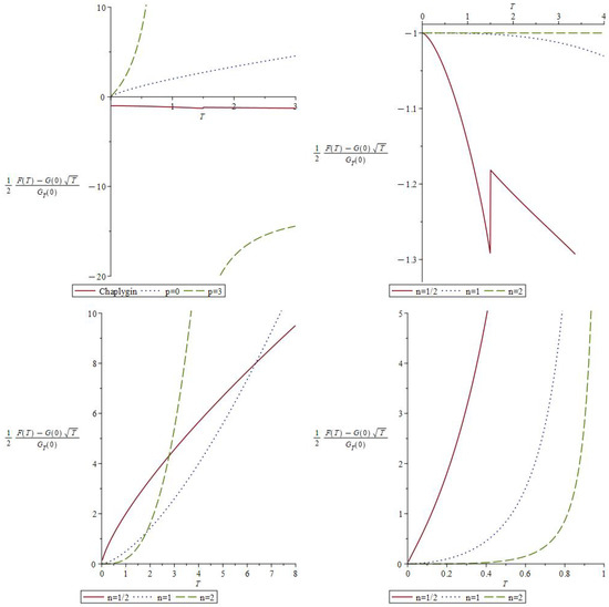
Figure 1.
Plot of flat cosmological teleparallel solutions for Chaplygin and polytropic cosmological gas sources (top left: and any p, top right: Chaplygin, bottom left: limit, bottom right: ).
For the spatially curved cases, we found some far-future approximated teleparallel solutions, all described by double power-law defined by the form of Equation (52). We only found the power in each cases after approximating Equations (50) and (59) for Chaplygin gas, and Equations (70) and (75) for general polytropic gas. A first feature is that the polytropic p-type teleparallel solutions do not contain any p-dependent term, as seen in Section 4.3 and Section 4.4 for solutions. The approximated polytropic teleparallel solutions are greatly simplified by parameter approximations agreeing to far future cosmological evolution models, as specifically in ref. [100]. The TEGR limit () is satisfied for most of subcases and for high-valued p-parameter values close to linear PF limit (and the CDM limit too). In this sense, the subcase represents more closely the expected and realistic cosmological models, and solutions are more comparable to those of refs. [56,98,99,100]. The future research will have to explicitly determine the p-parameter for any of flat and non-flat cosmological models.
5.2. Comparisons with Recent Experimental Results
However, the new Chaplygin and polytropic teleparallel solutions can be compared and tested with several experimental data sets from recent DE experiments such as Dark Energy Spectroscopic Instrument (DESI), and other Baryonic Data (BAO) and cosmological redshift measurements (-based measurements) [119,120,121,122,123,124,125]. The far future approximated teleparallel solution for cases can be easily compared to the mentioned DE data sets for baryonic as cosmological background types of data. The double power-law teleparallel solutions for far future universe evolution should also be compared with data for more precise and most relevant non-flat cosmological models. Investigating from this point, we can determine which solutions are the most realistic for universe models and explanations.
Therefore, we can never forget that the current paper primarily aims to develop and find by theoretical and mathematical means the most relevant teleparallel solutions for non-linear cosmological fluids such as Chaplygin and polytropic gases. In Section 3 and Section 4 we find the most relevant and easily verifiable new teleparallel solutions to be formally tested and compared with DESI or equivalent data sets. From this point, we can propose the main aim of future research to be comparing, by direct data fitting, these new teleparallel solutions with DE and background measurement as those made by the DESI collaboration [119,120,121,122,123]. We have seen that several of the new teleparallel solutions are also close to those found in refs [98,99,100], especially Equation (52)-based double power-law solutions found in Section 3.3, Section 3.4, Section 4, Section 4.1, Section 4.2, Section 4.3 and Section 4.4. These results will allow us to make good comparison with data sets in the future data fitting based works for determining which of the new solution classes are the most realistic for universe description.
Beyond the new teleparallel solution class determination, we will also be able to determine, by the same means, whether Chaplygin or polytropic fluid is more suitable for describing a DE-dominating universe with some amount of dust matter. We will be able to find the exact value of p and n parameters and also several other thermodynamic-based physical quantities for a DE dominating and expanding universe for a flat () and a non-flat () universe. We will be able to better confirm and/or adapt the CDM models to the data sets and by determining the most suitable new teleparallel solution models. Some recent similar studies using data comparison have been performed for more simple universe models cases using redshift , BAO and other similar data sets (see refs. [126,127,128] and refs. within). We will be able to use the scale factor a and determine the n-parameter possible values for the comparison with redshift measurements. Some data analysis techniques used in these mentioned works can be reused for future comparative works for the new teleparallel solutions found here. But the data comparison goes beyond the aims and scopes of the theoretical and mathematical physics based approach of the current paper. Nevertheless, the data fitting-based studies deserve to be performed in a near future and as suggested in some recent works for teleparallel -type extension solutions [62]. In the current work, we have all needed ingredients to achieve any future full data-based polytropic/Chaplygin fluid determination study.
6. Concluding Remarks
We will first conclude the current paper by stating that the flat cosmological teleparallel solutions are described by special functions, especially by hypergeometric functions plotted on the Figure 1 for Chaplygin () and polytropic limit and three gases. For the spatially curved cosmological teleparallel solutions are practically all approximated by a double power-law function described by Equation (52). The general polytropic solutions found in Section 4.3 and Section 4.4 are not p-dependent because of some dominating terms approximations. There is an important feature in the new solutions: no cosmological constant term in almost all the cases. The only exception are Equations (56) and (57) under the limit, leading to a simple polynomial with term. Under all previous considerations, we can claim that non-flat teleparallel solutions have some common points with those found for cosmological teleparallel and solutions found in refs [55,56,62], because we use the same coframe/spin-connection pair and ansatz. However, the current paper is a starting point to verify and test the new teleparallel solutions on recent experimental data sets as performed in very recent studies with this aim [126,127,128]. In the future, by using similar experimental data analysis approaches, we will need to formally compare the new solutions with DE, BAO and redshift experimental data sets. This will allow us to determine the most suitable classes of Chaplygin/polytropic teleparallel solutions for explaining and determining the acceleration of expansion magnitude, the polytropic level and several other related physical parameters of the universe as precise as possible.
Therefore, there are some perspectives for future research going beyond the current works. We can proceed, for example, with the same type of polytropic fluid sources for KS and static SS teleparallel spacetimes for new additional classes of solutions by using the same process and coframe ansatz approaches as in refs. [48,49,51,52]. We can also use the same TRW geometry, replace polytropic sources by an electromagnetic source, proceed by the same approach, and finally find the corresponding classes of teleparallel solutions. A last insight is that we will be able to study the Anti-deSitter (AdS) spacetimes in teleparallel gravity by using polytropic sources. However, we also need to investigate the polytropic principles in teleparallel gravity framework for possible symmetries and additional KVs. More physically, we will be able to elaborate a pure teleparallel quartessence models explaining the dark energy and the dark matter under an unified model. All these suggestions are feasible in the near future and will allow us to study the AdS wormholes and BHs solutions in teleparallel gravity.
Funding
This research received no external funding.
Data Availability Statement
The original contributions presented in this study are included in the article. Further inquiries can be directed to the corresponding author.
Conflicts of Interest
The authors declare no conflicts of interest.
References
- Lucas, T.G.; Obukhov, Y.; Pereira, J.G. Regularizing role of teleparallelism. Phys. Rev. D 2009, 80, 064043. [Google Scholar] [CrossRef]
- Krššák, M.; van den Hoogen, R.J.; Pereira, J.G.; Boehmer, C.G.; Coley, A.A. Teleparallel Theories of Gravity: Illuminating a Fully Invariant Approach. Class. Quantum Gravity 2019, 36, 183001. [Google Scholar] [CrossRef]
- Bahamonde, S.; Dialektopoulos, K.F.; Escamilla-Rivera, C.; Farrugia, G.; Gakis, V.; Hendry, M.; Hohmann, M.; Said, J.L.; Mifsud, J.; Di Valentino, E. Teleparallel Gravity: From Theory to Cosmology. Rep. Prog. Phys. 2023, 86, 026901. [Google Scholar] [CrossRef] [PubMed]
- Krssak, M.; Pereira, J.G. Spin Connection and Renormalization of Teleparallel Action. Eur. Phys. J. C 2015, 75, 519. [Google Scholar] [CrossRef]
- Coley, A.A.; van den Hoogen, R.J.; McNutt, D.D. Symmetry and Equivalence in Teleparallel Gravity. J. Math. Phys. 2020, 61, 072503. [Google Scholar] [CrossRef]
- McNutt, D.D.; Coley, A.A.; van den Hoogen, R.J. A frame based approach to computing symmetries with non-trivial isotropy groups. J. Math. Phys. 2023, 64, 032503. [Google Scholar] [CrossRef]
- Aldrovandi, R.; Pereira, J.G. Teleparallel Gravity, an Introduction; Springer: Berlin/Heidelberg, Germany, 2013. [Google Scholar]
- Olver, P. Equivalence, Invariants and Symmetry; Cambridge University Press: Cambridge, UK, 1995. [Google Scholar]
- Krššák, M.; Saridakis, E.N. The covariant formulation of f(T) gravity. Class. Quantum Gravity 2016, 33, 115009. [Google Scholar] [CrossRef]
- Ferraro, R.; Fiorini, F. Modified teleparallel gravity: Inflation without an inflation. Phys. Rev. D 2007, 75, 084031. [Google Scholar] [CrossRef]
- Ferraro, R.; Fiorini, F. On Born-Infeld Gravity in Weitzenbock spacetime. Phys. Rev. D 2008, 78, 124019. [Google Scholar] [CrossRef]
- Linder, E. Einstein’s Other Gravity and the Acceleration of the Universe. Phys. Rev. D 2010, 81, 127301, Erratum in Phys. Rev. D 2010, 82, 109902.. [Google Scholar] [CrossRef]
- Hayashi, K.; Shirafuji, T. New general relativity. Phys. Rev. D 1979, 19, 3524. [Google Scholar] [CrossRef]
- Jimenez, J.B.; Dialektopoulos, K.F. Non-Linear Obstructions for Consistent New General Relativity. J. Cosmol. Atroparticle Phys. 2020, 2020, 18. [Google Scholar] [CrossRef]
- Bahamonde, S.; Blixt, D.; Dialektopoulos, K.F.; Hell, A. Revisiting Stability in New General Relativity. Phys. Rev. D 2024, 111, 064080. [Google Scholar] [CrossRef]
- Heisenberg, L. Review on f(Q) Gravit. Phys. Rep. 2023, 1066, 1–78. [Google Scholar] [CrossRef]
- Heisenberg, L.; Hohmann, M.; Kuhn, S. Cosmological teleparallel perturbations. J. Cosmol. Astropart. Phys. 2024, 3, 63. [Google Scholar] [CrossRef]
- Flathmann, K.; Hohmann, M. Parametrized post-Newtonian limit of generalized scalar-nonmetricity theories of gravity. Phys. Rev. D 2022, 105, 044002. [Google Scholar] [CrossRef]
- Hohmann, M. General covariant symmetric teleparallel cosmology. Phys. Rev. D 2021, 104, 124077. [Google Scholar] [CrossRef]
- Jimenez, J.B.; Heisenberg, L.; Koivisto, T.S. The Geometrical Trinity of Gravity. Universe 2019, 5, 173. [Google Scholar] [CrossRef]
- Nakayama, Y. Geometrical trinity of unimodular gravity. Class. Quantum Gravity 2023, 40, 125005. [Google Scholar] [CrossRef]
- Xu, Y.; Li, G.; Harko, T.; Liang, S.-D. f(Q,T) gravity. Eur. Phys. J. C 2019, 79, 708. [Google Scholar] [CrossRef]
- Maurya, D.C.; Myrzakulov, R. Exact Cosmology in Myrzakulov Gravity. Eur. Phys. J. C 2024, 84, 625. [Google Scholar]
- Harko, T.; Lobo, F.S.N.; Nojiri, S.; Odintsov, S.D. f(R,T) gravity. Phys. Rev. D 2011, 84, 024020. [Google Scholar] [CrossRef]
- Momeni, D.; Myrzakulov, R. Myrzakulov Gravity in Vielbein Formalism: A Study in Weitzenböck Spacetime. Nucl. Phys. B 2025, 1015, 116903. [Google Scholar] [CrossRef]
- Maurya, D.C.; Yesmakhanova, K.; Myrzakulov, R.; Nugmanova, G. Myrzakulov F(T,Q) gravity: Cosmological implications and constraints. Phys. Scr. 2024, 99, 10. [Google Scholar] [CrossRef]
- Maurya, D.C.; Yesmakhanova, K.; Myrzakulov, R.; Nugmanova, G. FLRW Cosmology in Metric-Affine F(R,Q) Gravity. Chin. Phys. C 2024, 48, 125101. [Google Scholar] [CrossRef]
- Maurya, D.C.; Myrzakulov, R. Transit cosmological models in Myrzakulov F(R,T) gravity theory. Eur. Phys. J. C 2024, 84, 534. [Google Scholar] [CrossRef]
- Mandal, S.; Myrzakulov, N.; Sahoo, P.K.; Myrzakulov, R. Cosmological bouncing scenarios in symmetric teleparallel gravity. Eur. Phys. J. Plus 2021, 136, 760. [Google Scholar] [CrossRef]
- Golovnev, A.; Guzman, M.-J. Approaches to spherically symmetric solutions in f(T)-gravity. Universe 2021, 7, 121. [Google Scholar] [CrossRef]
- Golovnev, A. Issues of Lorentz-invariance in f(T)-gravity and calculations for spherically symmetric solutions. Class. Quantum Gravity 2021, 38, 197001. [Google Scholar] [CrossRef]
- DeBenedictis, A.; Ilijić, S.; Sossich, M. On spherically symmetric vacuum solutions and horizons in covariant f(T) gravity theory. Phys. Rev. D 2022, 105, 084020. [Google Scholar] [CrossRef]
- Bahamonde, S.; Camci, U. Exact Spherically Symmetric Solutions in Modified Teleparallel gravity. Symmetry 2019, 11, 1462. [Google Scholar] [CrossRef]
- Awad, A.; Golovnev, A.; Guzman, M.-J.; El Hanafy, W. Revisiting diagonal tetrads: New Black Hole solutions in f(T)-gravity. Eur. Phys. J. C 2022, 82, 972. [Google Scholar] [CrossRef]
- Bahamonde, S.; Golovnev, A.; Guzmán, M.-J.; Said, J.L.; Pfeifer, C. Black Holes in f(T,B) Gravity: Exact and Perturbed Solutions. J. Cosmol. Atroparticle Phys. 2022, 1, 037. [Google Scholar] [CrossRef]
- Bahamonde, S.; Faraji, S.; Hackmann, E.; Pfeifer, C. Thick accretion disk configurations in the Born-Infeld teleparallel gravity. Phys. Rev. D 2022, 106, 084046. [Google Scholar] [CrossRef]
- Nashed, G.G.L. Quadratic and cubic spherically symmetric black holes in the modified teleparallel equivalent of general relativity: Energy and thermodynamics. Class. Quantum Gravity 2021, 38, 125004. [Google Scholar] [CrossRef]
- Pfeifer, C.; Schuster, S. Static spherically symmetric black holes in weak f(T)-gravity. Universe 2021, 7, 153. [Google Scholar] [CrossRef]
- El Hanafy, W.; Nashed, G.G.L. Exact Teleparallel Gravity of Binary Black Holes. Astrophys. Space Sci. 2016, 361, 68. [Google Scholar] [CrossRef]
- Aftergood, J.; DeBenedictis, A. Matter Conditions for Regular Black Holes in f(T) Gravity. Phys. Rev. D 2014, 90, 124006. [Google Scholar] [CrossRef]
- Bahamonde, S.; Doneva, D.D.; Ducobu, L.; Pfeifer, C.; Yazadjiev, S.S. Spontaneous Scalarization of Black Holes in Gauss-Bonnet Teleparallel Gravity. Phys. Rev. D 2023, 107, 104013. [Google Scholar] [CrossRef]
- Bahamonde, S.; Ducobu, L.; Pfeifer, C. Scalarized Black Holes in Teleparallel Gravity. J. Cosmol. Atroparticle Phys. 2022, 2022, 18. [Google Scholar] [CrossRef]
- Iorio, L.; Radicella, N.; Ruggiero, M.L. Constraining f(T) gravity in the Solar System. J. Cosmol. Atroparticle Phys. 2015, 2015, 21. [Google Scholar] [CrossRef]
- Pradhan, S.; Bhar, P.; Mandal, S.; Sahoo, P.K.; Bamba, K. The Stability of Anisotropic Compact Stars Influenced by Dark Matter under Teleparallel Gravity: An Extended Gravitational Deformation Approach. Eur. Phys. J. C 2025, 85, 127. [Google Scholar] [CrossRef]
- Mohanty, D.; Ghosh, S.; Sahoo, P.K. Charged gravastar model in noncommutative geometry under f(T) gravity. Phys. Dark Universe 2025, 46, 101692. [Google Scholar] [CrossRef]
- Calza, M.; Sebastiani, L. A class of static spherically symmetric solutions in f(T)-gravity. Eur. Phys. J. C 2024, 84, 476. [Google Scholar] [CrossRef]
- Coley, A.A.; Landry, A.; van den Hoogen, R.J.; McNutt, D.D. Spherically symmetric teleparallel geometries. Eur. Phys. J. C 2024, 84, 334. [Google Scholar] [CrossRef] [PubMed]
- Landry, A. Static spherically symmetric perfect fluid solutions in teleparallel F(T) gravity. Axioms 2024, 13, 333. [Google Scholar] [CrossRef]
- Landry, A. Kantowski-Sachs spherically symmetric solutions in teleparallel F(T) gravity. Symmetry 2024, 16, 953. [Google Scholar] [CrossRef]
- van den Hoogen, R.J.; Forance, H. Teleparallel Geometry with Spherical Symmetry: The diagonal and proper frames. J. Cosmol. Astrophys. 2024, 11, 033. [Google Scholar] [CrossRef]
- Landry, A. Scalar field Kantowski-Sachs spacetime solutions in teleparallel F(T) gravity. Universe 2025, 11, 26. [Google Scholar] [CrossRef]
- Landry, A. Scalar Field Static Spherically Symmetric Solutions in Teleparallel F(T) Gravity. Mathematics 2025, 13, 1003. [Google Scholar] [CrossRef]
- Coley, A.A.; Landry, A.; van den Hoogen, R.J.; McNutt, D.D. Generalized Teleparallel de Sitter geometries. Eur. Phys. J. C 2023, 83, 977. [Google Scholar] [CrossRef] [PubMed]
- Golovnev, A.; Guzman, M.-J. Bianchi identities in f(T)-gravity: Paving the way to confrontation with astrophysics. Phys. Lett. B 2020, 810, 135806. [Google Scholar] [CrossRef]
- Landry, A. Scalar field source Teleparallel Robertson-Walker F(T)-gravity solutions. Mathematics 2025, 13, 374. [Google Scholar] [CrossRef]
- Coley, A.A.; Landry, A.; Gholami, F. Teleparallel Robertson-Walker Geometries and Applications. Universe 2023, 9, 454. [Google Scholar] [CrossRef]
- Coley, A.A.; van den Hoogen, R.J.; McNutt, D.D. Symmetric Teleparallel Geometries. Class. Quantum Gravity 2022, 39, 22LT01. [Google Scholar] [CrossRef]
- Aldrovandi, R.; Cuzinatto, R.R.; Medeiros, L.G. Analytic solutions for the Λ-FRW Model. Found. Phys. 2006, 36, 1736–1752. [Google Scholar] [CrossRef]
- Casalino, A.; Sanna, B.; Sebastiani, L.; Zerbini, S. Bounce Models within Teleparallel modified gravity. Phys. Rev. D 2021, 103, 023514. [Google Scholar] [CrossRef]
- Capozziello, S.; Luongo, O.; Pincak, R.; Ravanpak, A. Cosmic acceleration in non-flat f(T) cosmology. Gen. Relativ. Gravit. 2018, 50, 53. [Google Scholar] [CrossRef]
- Bahamonde, S.; Dialektopoulos, K.F.; Hohmann, M.; Said, J.L.; Pfeifer, C.; Saridakis, E.N. Perturbations in Non-Flat Cosmology for f(T) gravity. Eur. Phys. J. C 2023, 83, 193. [Google Scholar] [CrossRef]
- Gholami, F.; Landry, A. Cosmological solutions in teleparallel F(T,B) gravity. Symmetry 2025, 17, 60. [Google Scholar] [CrossRef]
- Hohmann, M.; Järv, L.; Krššák, M.; Pfeifer, C. Modified teleparallel theories of gravity in symmetric spacetimes. Phys. Rev. D 2019, 2019 100, 084002. [Google Scholar] [CrossRef]
- Cai, Y.-F.; Capozziello, S.; De Laurentis, M.; Saridakis, E.N. f(T) teleparallel gravity and cosmology. Rep. Prog. Phys. 2016, 79, 106901. [Google Scholar] [CrossRef]
- Dixit, A.; Pradhan, A. Bulk Viscous Flat FLRW Model with Observational Constraints in f(T,B) Gravity. Universe 2022, 8, 650. [Google Scholar] [CrossRef]
- Chokyi, K.K.; Chattopadhyay, S. Cosmological Models within f(T,B) Gravity in a Holographic Framework. Particles 2024, 7, 856–878. [Google Scholar] [CrossRef]
- Hawking, S.W.; Ellis, G.F.R. The Large Scale Structure of Space-Time; Cambridge University Press: Cambridge, UK, 2010. [Google Scholar]
- Bohmer, C.G.; d’Alfonso del Sordo, A. Cosmological fluids with boundary term couplings. Gen. Relativ. Gravit. 2024, 56, 75. [Google Scholar] [CrossRef]
- Bahamonde, S.; Bohmer, C.G.; Carloni, S.; Copeland, E.J.; Fang, W.; Tamanini, N. Dynamical systems applied to cosmology: Dark energy and modified gravity. Phys. Rep. 2018, 775–777, 1–122. [Google Scholar] [CrossRef]
- Zlatev, I.; Wang, L.; Steinhardt, P. Quintessence, Cosmic Coincidence, and the Cosmological Constant. Phys. Rev. Lett. 1999, 82, 896. [Google Scholar] [CrossRef]
- Steinhardt, P.; Wang, L.; Zlatev, I. Cosmological tracking solutions. Phys. Rev. D 1999, 59, 123504. [Google Scholar] [CrossRef]
- Caldwell, R.R.; Dave, R.; Steinhardt, P. Cosmological Imprint of an Energy Component with General Equation of State. Phys. Rev. Lett. 1998, 80, 1582. [Google Scholar] [CrossRef]
- Carroll, S.M. Quintessence and the Rest of the World. Phys. Rev. Lett. 1998, 81, 3067. [Google Scholar] [CrossRef]
- Doran, M.; Lilley, M.; Schwindt, J.; Wetterich, C. Quintessence and the Separation of CMB Peaks. Astrophys. J. 2001, 559, 501. [Google Scholar] [CrossRef]
- Zeng, X.-X.; Chen, D.-Y.; Li, L.-F. Holographic thermalization and gravitational collapse in the spacetime dominated by quintessence dark energy. Phys. Rev. D 2015, 91, 046005. [Google Scholar] [CrossRef]
- Chakraborty, S.; Mishra, S.; Chakraborty, S. Dynamical system analysis of quintessence dark energy model. Int. J. Geom. Methods Mod. Phys. 2025, 22, 2450250. [Google Scholar] [CrossRef]
- Shlivko, D.; Steinhardt, P.J. Assessing observational constraints on dark energy. Phys. Lett. B 2024, 855, 138826. [Google Scholar] [CrossRef]
- Ratra, B.; Peebles, P.J.E. Cosmological consequences of a rolling homogeneous scalar field. Phys. Rev. D 1988, 37, 3406. [Google Scholar] [CrossRef] [PubMed]
- Wolf, W.J.; Ferreira, P.G. Underdetermination of dark energy. Phys. Rev. D 2023, 108, 103519. [Google Scholar] [CrossRef]
- Wolf, W.J.; García-García, C.; Bartlett, D.J.; Ferreira, P.G. Scant evidence for thawing quintessence. Phys. Rev. D 2024, 110, 083528. [Google Scholar] [CrossRef]
- Wolf, W.J.; Ferreira, P.G.; García-García, C. Matching current observational constraints with nonminimally coupled dark energy. Phys. Rev. D 2025, 111, L041303. [Google Scholar] [CrossRef]
- Wetterich, C. Cosmology and the Fate of Dilatation Symmetry. Nucl. Phys. B 1988, 302, 668. [Google Scholar] [CrossRef]
- Chiba, T.; Okabe, T.; Yamaguchi, M. Kinetically Driven Quintessence. Phys. Rev. D 2000, 62, 023511. [Google Scholar] [CrossRef]
- Carroll, S.M.; Hoffman, M.; Trodden, M. Can the dark energy equation-of-state parameter w be less than −1? Phys. Rev. D 2003, 68, 023509. [Google Scholar] [CrossRef]
- Caldwell, R.R. A phantom menace? Cosmological consequences of a dark energy component with super-negative equation of state. Phys. Lett. B 2002, 545, 23. [Google Scholar] [CrossRef]
- Farnes, J.S. A Unifying Theory of Dark Energy and Dark Matter: Negative Masses and Matter Creation within a Modified ΛCDM Framework. Astron. Astrophys. 2018, 620, A92. [Google Scholar] [CrossRef]
- Baum, L.; Frampton, P.H. Turnaround in Cyclic Cosmology. Phys. Rev. Lett. 2007, 98, 071301. [Google Scholar] [CrossRef]
- Hu, W. Crossing the Phantom Divide: Dark Energy Internal Degrees of Freedom. Phys. Rev. D 2005, 71, 047301. [Google Scholar] [CrossRef]
- Karimzadeh, S.; Shojaee, R. Phantom-Like Behavior in Modified Teleparallel Gravity. Adv. High Energy Phys. 2019, 2019, 4026856. [Google Scholar] [CrossRef]
- Pati, L.; Kadam, S.A.; Tripathy, S.K.; Mishra, B. Rip cosmological models in extended symmetric teleparallel gravity. Phys. Dark Universe 2022, 35, 100925. [Google Scholar] [CrossRef]
- Kucukakca, Y.; Akbarieh, A.R.; Ashrafi, S. Exact solutions in teleparallel dark energy model. Chin. J. Phys. 2023, 82, 47. [Google Scholar] [CrossRef]
- Cai, Y.-F.; Saridakis, E.N.; Setare, M.R.; Xia, J.-Q. Quintom Cosmology: Theoretical implications and observations. Phys. Rep. 2010, 493, 1. [Google Scholar] [CrossRef]
- Guo, Z.-K.; Piao, Y.-S.; Zhang, X.; Zhang, Y.-Z. Cosmological evolution of a quintom model of dark energy. Phys. Lett. B 2005, 608, 177. [Google Scholar] [CrossRef]
- Feng, B.; Li, M.; Piao, Y.-S.; Zhang, X. Oscillating quintom and the recurrent universe. Phys. Lett. B 2006, 634, 101. [Google Scholar] [CrossRef]
- Mishra, S.; Chakraborty, S. Dynamical system analysis of quintom dark energy model. Eur. Phys. J. C 2018, 78, 917. [Google Scholar] [CrossRef]
- Tot, J.; Coley, A.A.; Yildrim, B.; Leon, G. The dynamics of scalar-field Quintom cosmological models. Phys. Dark Universe 2023, 39, 101155. [Google Scholar] [CrossRef]
- Bahamonde, S.; Marciu, M.; Rudra, P. Generalised teleparallel quintom dark energy non-minimally coupled with the scalar torsion and a boundary term. J. Cosmol. Astropart. Phys. 2018, 4, 56. [Google Scholar] [CrossRef]
- Myrzakulov, R. Accelerating universe from F(T) gravity. Eur. Phys. J. C 2011, 71, 1752. [Google Scholar] [CrossRef]
- Myrzakulov, R.; Saez-Gomez, D.; Tsyba, P. Cosmological solutions in F(T) gravity with the presence of spinor fields. Int. J. Geom. Methods Mod. Phys. 2015, 12, 1550023. [Google Scholar] [CrossRef]
- Paliathanasis, A. F(T) Cosmology with Nonzero Curvature. Mod. Phys. Lett. A 2021, 36, 2150261. [Google Scholar] [CrossRef]
- Gorini, V.; Kamenshchik, A.Y.; Moschella, U.; Pasquier, V. Chaplygin gas as a model for dark energy. In Proceedings of the Tenth Marcel Grossmann Meeting: On Recent Developments in Theoretical and Experimental General Relativity, Gravitation and Relativistic Field Theories (In 3 Volumes), Rio de Janeiro, Brazil, 20–26 July 2003; p. 840. [Google Scholar]
- Bento, M.C.; Bertolami, O.; Sen, A.A. Generalized Chaplygin Gas Model: Dark Energy-Dark Matter Unification and CMBR Constraints. Gen. Relativ. Gravit. 2003, 35, 2063. [Google Scholar] [CrossRef]
- Bilić, N.; Tuppe, G.B.; Viollier, R.D. Unification of dark matter and dark energy: The inhomogeneous Chaplygin gas. Phys. Lett. B 2002, 535, 17. [Google Scholar] [CrossRef]
- Makler, M.; de Oliveira, S.Q.; Waga, I. Observational constraints on Chaplygin quartessence: Background results. Phys. Rev. D 2003, 68, 123521. [Google Scholar] [CrossRef]
- Zhu, Z.-H. Generalized Chaplygin gas as a unified scenario of dark matter/energy: Observational constraints. Astron. Astrophys. 2004, 423, 421. [Google Scholar] [CrossRef]
- Karami, K.; Ghaffari, S.; Fehri, J. Interacting polytropic gas model of phantom dark energy in non-flat universe. Eur. Phys. J. C 2009, 64, 85. [Google Scholar] [CrossRef]
- Karami, K.; Safari, Z.; Asadzadeh, S. Cosmological constraints on polytropic gas model. Int. J. Theor. Phys. 2014, 53, 1248. [Google Scholar]
- Karami, K.; Abdolmaleki, A. Reconstructing interacting new agegraphic polytropic gas model in non-flat FRW universe. Astrophys. Space Sci. 2010, 330, 133. [Google Scholar] [CrossRef]
- Karami, K.; Khaledian, M.S. Polytropic and Chaplygin f(R)-gravity models. Int. J. Mod. Phys. D 2012, 21, 1250083. [Google Scholar] [CrossRef]
- Banerjee, S.; Paul, A. Effect of Accretion on the evolution of Primordial Black Holes in the context of Modified Gravity Theories. arXiv 2024, arXiv:2406.04605. [Google Scholar] [CrossRef]
- Aboueisha, M.S.; Nouh, M.I.; Abdel-Salam, E.A.-B.; Kamel, T.M.; Beheary, M.M.; Gadallah, K.A.K. Analysis of the Fractional Relativistic Polytropic Gas Sphere. Sci. Rep. 2023, 13, 14304. [Google Scholar] [CrossRef]
- Cardenas, V.H.; Cruz, M. Emulating dark energy models with known equation of state via the created cold dark matter scenario. Phys. Dark Universe 2024, 44, 101452. [Google Scholar] [CrossRef]
- Jia, Y.; He, T.-Y.; Wang, W.-Q.; Han, Z.-W.; Yang, R.-J. Accretion of matter by a Charged dilaton black hole. Eur. Phys. J. C 2024, 84, 501. [Google Scholar] [CrossRef]
- Arun, K.; Gudennavar, S.B.; Sivaram, C. Dark matter, dark energy, and alternate models: A review. Adv. Space Res. 2017, 60, 166. [Google Scholar] [CrossRef]
- Iosifidis, D. Cosmological Hyperfluids, Torsion and Non-metricity. Eur. Phys. J. C 2020, 80, 1042. [Google Scholar] [CrossRef]
- Heisenberg, L.; Hohmann, M.; Kuhn, S. Homogeneous and isotropic cosmology in general teleparallel gravity. Eur. Phys. J. C 2023, 83, 315. [Google Scholar] [CrossRef] [PubMed]
- Heisenberg, L.; Hohmann, M. Gauge-invariant cosmological perturbations in general teleparallel gravity. Eur. Phys. J. C 2024, 84, 462. [Google Scholar] [CrossRef]
- Kontou, E.-A.; Sanders, K. Energy conditions in general relativity and quantum field theory. Class. Quantum Gravity 2020, 37, 193001. [Google Scholar] [CrossRef]
- DESI Collaboration. The Dark Energy Survey: Cosmology Results With 1500 New High-redshift Type Ia Supernovae Using The Full 5-year Dataset. Astrophys. J. Lett. 2024, 973, L14. [Google Scholar] [CrossRef]
- DESI Collaboration. DESI 2024 VI: Cosmological Constraints from the Measurements of Baryon Acoustic Oscillations. J. Cosmol. Astropart. Phys. 2025, 2, 21. [Google Scholar]
- DESI Collaboration. Dark Energy Survey: Implications for cosmological expansion models from the final DES Baryon Acoustic Oscillation and Supernova data. arXiv 2025, arXiv:2503.06712. [Google Scholar]
- DESI Collaboration. DESI DR2 Results II: Measurements of Baryon Acoustic Oscillations and Cosmological Constraint. arXiv arXiv:2503.14738. [CrossRef]
- DESI Collaboration. DESI DR2 Results I: Baryon Acoustic Oscillations from the Lyman Alpha Forest. Phys. Rev. D, 2025; in press. [Google Scholar]
- Notari, A.; Redi, M.; Tesi, A. BAO vs. SN evidence for evolving dark energy. J. Cosmol. Astropart. Phys. 2025, 4, 48. [Google Scholar] [CrossRef]
- Berti, M.; Bellini, E.; Bonvin, C.; Kunz, M.; Viel, M.; Zumalacarregui, M. Reconstructing the dark energy density in light of DESI BAO observations. Phys. Rev. D 2025, 112, 023518. [Google Scholar] [CrossRef]
- Escamilla-Rivera, C.; Sandoval-Orozco, R. f(T) gravity after DESI Baryon acoustic oscillation and DES supernovae 2024 data. J. High Energy Astrophys. 2024, 42, 217–221. [Google Scholar] [CrossRef]
- Aguilar, A.; Escamilla-Rivera, C.; Said, J.L.; Mifsud, J. Non-fluid like Boltzmann code architecture for early times f(T) cosmologies. arXiv 2024, arXiv:2403.13708. [Google Scholar]
- Sandoval-Orozco, R.; Escamilla-Rivera, C.; Briffa, R.; Said, J.L. Testing f(T) cosmologies with HII Hubble diagram and CMB distance priors. Phys. Dark Universe 2024, 46, 101641. [Google Scholar] [CrossRef]

Disclaimer/Publisher’s Note: The statements, opinions and data contained in all publications are solely those of the individual author(s) and contributor(s) and not of MDPI and/or the editor(s). MDPI and/or the editor(s) disclaim responsibility for any injury to people or property resulting from any ideas, methods, instructions or products referred to in the content. |
© 2025 by the author. Licensee MDPI, Basel, Switzerland. This article is an open access article distributed under the terms and conditions of the Creative Commons Attribution (CC BY) license (https://creativecommons.org/licenses/by/4.0/).