Article

Bayesian Optimization for the Synthesis of Generalized State-Feedback Controllers in Underactuated Systems

by
Miguel A. Solis
1,
Sinnu S. Thomas
2,
Christian A. Choque-Surco
3,*,
Edgar A. Taya-Acosta
4 and
Francisca Coiro
5
1
Faculty of Engineering, Universidad Andres Bello, Santiago 7500971, Chile
2
School of Computer Science and Engineering, Digital University Kerala (Formerly IIITMK), Kerala 695317, India
3
School of Computer and Systems Engineering, Jorge Basadre Grohmann National University, Tacna 23001, Peru
4
Academic Department of Computer and Systems Engineering, Jorge Basadre Grohmann National University, Tacna 23001, Peru
5
Faculty of Education, Pontificia Universidad Catolica de Valparaiso, Valparaiso 2530388, Chile
*
Author to whom correspondence should be addressed.
Mathematics 2025, 13(19), 3139; https://doi.org/10.3390/math13193139
Submission received: 1 July 2025 / Revised: 27 July 2025 / Accepted: 2 August 2025 / Published: 1 October 2025
(This article belongs to the Special Issue New Advances in Control Theory and Its Applications)

Abstract

Underactuated systems, such as rotary and double inverted pendulums, challenge traditional control due to nonlinear dynamics and limited actuation. Classical methods like state-feedback and Linear Quadratic Regulators (LQRs) are commonly used but often require high gains, leading to excessive control effort, poor energy efficiency, and reduced robustness. This article proposes a generalized state-feedback controller with its own internal dynamics, offering greater design flexibility. To automate tuning and avoid manual calibration, we apply Bayesian Optimization (BO), a data-efficient strategy for optimizing closed-loop performance. The proposed method is evaluated on two benchmark underactuated systems, including one in simulation and one in a physical setup. Compared with standard LQR designs, the BO-tuned state-feedback controller achieves a reduction of approximately 20% in control signal amplitude while maintaining comparable settling times. These results highlight the advantages of combining model-based control with automatic hyperparameter optimization, achieving efficient regulation of underactuated systems without increasing design complexity.

1. Introduction

Underactuated systems pose a challenging problem, as their corresponding controllers must generate control signals that drive a given state to zero without necessarily being directly linked to an actuator, while also being capable of rejecting disturbances and handling model uncertainties. These systems are attractive due to their wide range of applications in areas such as aerospace and robotics [1,2,3].
State-feedback controllers are often preferred for their simple structure, typically consisting of a feedback gain. However, the dynamics of the plant can sometimes result in a static feedback controller requiring higher gains than desired, leading to increased control costs such as higher power consumption. In this work, we demonstrate the effectiveness of applying a generalized state-feedback structure to underactuated control systems. This approach can achieve similar performance to a traditional state-feedback controller while reducing control cost by introducing additional parameters into the model.
One of the most widely used benchmark experiments in the field of underactuated mechanical systems is the rotary inverted pendulum, which has a nonlinear model that can be approximated as linear around its unstable upright position. This plant consists of a controlled arm rotating around a central axis and a pendulum attached to one end of the arm. It enables the study of nonlinear dynamics in simplified models that can also be physically constructed, offering improved reproducibility.
The Linear Quadratic Regulator (LQR) is a well-known problem in linear control theory, where the system is assumed to be linear and the performance index is defined by a quadratic function [4]. The solution to the LQR problem is obtained by solving an Algebraic Riccati Equation. The Linear Quadratic Tracking (LQT) problem also assumes linear process dynamics and a quadratic cost function, but its objective is to design a controller that tracks an exogenous reference signal, making LQR a special case of LQT.
State-feedback controllers are favored not only for their simplicity but also for their low computational cost in generating control signals. The generalized state-feedback controller extends the classical structure by introducing an additional degree of freedom, though at the expense of extra parameters that must be tuned.
We address the controller design problem through automatic tuning using Bayesian Optimization, a global optimization method suitable for multi-modal, computationally expensive black-box functions. This contrasts with gradient-based techniques, which are more prone to getting stuck in local optima. Our work builds on the analysis in [5], where the generalized state-feedback controller was tuned using reinforcement learning and applied solely to the rotary inverted pendulum. In this paper, we extend that approach to include analysis of the double inverted pendulum as well.
The main contribution of this work is the integration of a generalized state-feedback controller structure with Bayesian Optimization to address the control of underactuated systems. Unlike classical LQR methods, the proposed controller includes internal dynamic states and additional degrees of freedom, allowing enhanced flexibility and energy efficiency. Bayesian Optimization is employed as a data-efficient strategy to automatically tune the controller parameters based on spectral radius minimization, avoiding manual calibration. This hybrid approach combines the theoretical rigor of model-based control with the adaptability of learning-based optimization. The method is validated on two benchmark systems—the physical rotary inverted pendulum and a simulated double inverted pendulum—demonstrating improved performance in terms of control effort and error reduction compared with traditional techniques.
The remainder of this article is structured as follows: Section 2 reviews related work on state-feedback controllers and their applications to underactuated systems. Section 3 presents the rotary inverted pendulum with its linear model obtained from a phenomenological analysis, the corresponding linearization, and the model for the double inverted pendulum. It concludes with the formulation of the Linear Quadratic Regulator problem and classical state-feedback control. Section 5 describes the Bayesian Optimization algorithm applied to tune the parameters of the generalized state-feedback controller. The results are reported in Section 6, followed by final remarks and conclusions in Section 7.

2. Literature Review

2.1. Underactuated Systems

The control community has extensively studied underactuated systems and introduced benchmark problems, such as the cart-pole system, where control requires not only stabilizing the pendulum in an unstable position but also managing the displacement of the cart, making the control problem more complex [6]. Other underactuated mechanical systems with simplified models also exist, allowing researchers to capture the essence of the problem without the complexity found in real-world applications—such as the rotary inverted pendulum (RIP), also known as the Furuta pendulum [7].
Various control techniques have been applied to underactuated systems. For example, Cui et al. [8] proposed a Fast Particle Swarm Optimization (Fast-PSO) algorithm, which improves the convergence speed and robustness of the original PSO through adaptive velocity control. Although not originally applied to the rotary inverted pendulum, this algorithm represents a class of optimization strategies that have inspired controller tuning methods for nonlinear and underactuated systems.
Similarly, Kong et al. [9] proposed an asymmetric bounded neural control method for uncertain underactuated systems, using both state and output feedback. Their approach addresses robustness and adaptability in the presence of model uncertainties. The controller’s performance is validated through simulations and compared with conventional methods, demonstrating improved stability and tracking performance under significant uncertainty.
Artificial neural networks can also enhance other learning approaches, such as reinforcement learning algorithms [10], which have been widely used to solve the Linear Quadratic Regulator (LQR) problem. In this case, the system is assumed to be linear, and the performance index is expressed as a quadratic function [4]. The solution is obtained by solving an Algebraic Riccati Equation (ARE). The Linear Quadratic Tracking (LQT) problem similarly assumes a linear process model and a quadratic cost function, but its objective is to design a controller such that the measured output follows an exogenous reference signal. The LQR can be considered a special case of the LQT problem.
However, the LQT problem has received limited attention in the literature, mainly because, for most reference signals, the infinite-horizon cost becomes unbounded [11]. Qin and Zhang tackled this issue in the continuous-time domain by solving an augmented ARE [12], while Kiumarsi et al. adopted a similar approach for the discrete-time case using a Q-learning algorithm [13,14]. Their results show that the proposed method achieves good stability and trajectory tracking performance even in the presence of unknown dynamics.
Although these approaches are innovative and do not require full model knowledge, they often involve high computational effort. The generalized state-feedback controllers proposed in this work include three additional design parameters, yet they yield lower-amplitude control signals and are expected to enhance convergence and system stationarity.
In contrast with model-free schemes, state-feedback controllers allow for systematic design using known dynamics and can provide closed-loop stability guarantees. However, their performance is highly dependent on the quality of gain selection. This work addresses that limitation by incorporating a generalized state-feedback structure with automated tuning to retain stability guarantees while improving adaptability.
Recent approaches have explored model-free and hybrid control schemes such as intelligent PID (iPID), sigmoid-based PID controllers, neuroendocrine PID, and brain-emotional-learning-based intelligent controllers (BELBICs) [15,16,17]. These methods aim to improve tracking and robustness in nonlinear systems without relying on full model knowledge. While effective in some contexts, they typically require extensive tuning or simulation-based calibration and may not offer formal guarantees on stability or optimality.

2.2. Bayesian Optimization

The Bayesian Optimization (BO) method [18] constructs a representation of the unknown objective function using a surrogate model and then optimizes it via iterative sampling, guided by an acquisition function defined based on the surrogate model [19,20,21]. BO has been extensively studied for the optimization of unknown functions across various domains. Its success relies heavily on the choice of acquisition function to identify the most promising regions of the search space. To prevent unnecessary evaluations, Nguyen et al. [22] proposed convergence criteria for acquisition functions.
BO has been successfully applied to a wide range of applications, including machine learning [23], analog circuit design [24], voltage fault diagnosis [25], aerospace engineering [26], pharmaceutical research [27], gas–liquid separation in laboratories [28], multi-objective optimization [29], free-electron lasers [30], and autonomous systems.
Alternative optimization methods—such as improved sparrow search algorithms, particle swarm variants, and neuro-fuzzy tuning—have been applied to controller design in complex systems [31,32]. While powerful, these heuristics often lack convergence guarantees and require extensive trial runs. Bayesian Optimization, by contrast, is particularly suited for tuning in low-sample, expensive-to-evaluate contexts such as control design, offering principled convergence and efficient exploration–exploitation trade-offs.
In this work, Bayesian Optimization (BO) is employed to tune the gain matrices of a state-feedback controller such that the resulting closed-loop system places its eigenvalues near a set of desired locations. The optimization problem is formulated as the minimization of a scalar cost function, which quantifies the deviation between the current and target eigenvalues, reflecting the dynamic performance of the system. The BO algorithm models this objective via a Gaussian Process (GP), which provides a probabilistic estimate of the function and its uncertainty across the parameter space. At each iteration, candidate gain parameters are selected by optimizing an acquisition function—specifically, the Expected Improvement (EI)—which guides the search by trading off between exploration (uncertain areas) and exploitation (promising low-cost areas).
The Expected Improvement at a candidate point x is defined as
EI ( x ) = E max ( f min f ( x ) , 0 ) ,
where f min is the best (i.e., minimum) observed value of the objective function so far.
Given the GP posterior mean μ ( x ) and standard deviation σ ( x ) , the EI can be expressed in closed form as
EI ( x ) = ( f min μ ( x ) ) Φ f min μ ( x ) σ ( x ) + σ ( x ) ϕ f min μ ( x ) σ ( x ) ,
where Φ ( · ) and ϕ ( · ) denote the cumulative distribution function and probability density function of the standard normal distribution, respectively. This formulation encourages sampling in regions that either offer potentially better solutions (exploitation) or where the model is uncertain (exploration).
At each iteration, the selected parameters are used to construct the closed-loop system, compute its eigenvalues, and evaluate the cost function. These data are used to update the surrogate model, thereby refining the search landscape.
The procedure continues until a stopping criterion is satisfied. In this work, the algorithm terminates after a fixed number of iterations, although, in general, stopping criteria may also include convergence of the objective value, stabilization of the acquisition function, or practical constraints such as computational budget or runtime limits [33,34].

3. Theoretical Framework

3.1. Underactuated Systems

The control community has extensively studied underactuated systems and introduced benchmark problems, such as the cart-pole system, where control requires not only stabilizing the pendulum in its unstable position but also managing the displacement of the cart—making the control problem more complex [6]. Other underactuated mechanical systems with simplified models also exist, allowing researchers to capture the essence of the problem without the complexity of real-world applications—such as the rotary inverted pendulum (RIP), also known as the Furuta pendulum [7].
Consider a second-order, controllable dynamical system given by
q ¨ = f ( q , q ˙ , u , t ) ,
where u is the control input vector; q and q ˙ denote the position and velocity vectors, respectively; and t represents the possible time dependence of the acceleration vector q ¨ . In the case considered in this study—where the dynamics are affine in the commanded torque—the arbitrary function f in Equation (3) can be rewritten using the two functions f 1 and f 2 as
q ¨ = f 1 ( q , q ˙ , t ) + f 2 ( q , q ˙ , t ) u .
A system described in Equation (3) is formally defined as underactuated in the configuration ( q , q ˙ , t ) if it is not possible to generate instantaneous acceleration in an arbitrary direction, i.e.,
rank ( f 2 ( q , q ˙ , t ) ) < dim ( q ) ,
where dim ( M ) denotes the dimension of matrix M, and rank ( M ) refers to the maximum number of linearly independent columns in M.

3.2. Rotary Inverted Pendulum

The rotary inverted pendulum (RIP), also referred to as the Furuta pendulum, is a classic example of an underactuated system, as shown in Figure 1. The system consists of an arm in the horizontal plane that rotates around a central axis and a pendulum attached to one end of the arm, rotating in the vertical plane. This particular setup offers a platform for investigating the nonlinear dynamics of simplified models that are feasible to construct physically, resulting in mechatronic systems with improved reproducibility.
As shown in Figure 1, a DC motor controls the arm position, measured by θ 0 , through the armature voltage. Its main parameters are the armature resistance and inductance, denoted by R a and L a , respectively.

3.3. Model Formulation for the Rotary Inverted Pendulum

We define the parameters { l p , m p , I p , θ 1 } , where l p is the distance from the pendulum’s rotation axis to its center of mass, m p is the mass of the pendulum, I p is its moment of inertia, and θ 1 is its angular position. The arm has radius r and moment of inertia I a , and a counterweight of mass m c brings the center of mass of the rotating arm to a height h. The rotation angle of the arm is denoted by θ 0 . A detailed description of all parameters and their values for the physical prototype is shown in Table 1, derived from a phenomenological analysis consistent with the actual system [35].
The Lagrangian L ( θ , θ ˙ ) is given by
L ( q , q ˙ ) = E k ( q , q ˙ ) E p ( q , q ˙ ) ,
where E k and E p denote the kinetic and potential energies, respectively, and θ is the generalized coordinates vector, θ = θ 0 θ 1 .
The kinetic energy of the pendulum includes both translational and rotational components, while the arm’s kinetic energy includes rotational and tangential terms, as follows:
E k = 1 2 J ^ 0 θ ˙ 0 2 + 1 2 J ^ 1 θ ˙ 1 2 + 1 2 m p l p 2 θ ˙ 0 2 sin 2 ( θ 1 ) m p r l p θ ˙ 0 θ ˙ 1 cos ( θ 1 ) ,
where θ ˙ 0 and θ ˙ 1 are the angular velocities of the arm and pendulum, respectively.
The equivalent angular masses of the arm and pendulum, J ^ 0 and J ^ 1 , are given by
J ^ 0 = I a + r 2 ( m p + m c ) ,
J ^ 1 = I p + m p l p 2 ,
while the potential energy is defined by the pendulum and counterweight masses, as follows:
E p = m p g l p cos ( θ 1 ) + m c g h .
Then, according to the Euler–Lagrange equation,
t L q ˙ i L q i = τ i , i = θ 0 , θ 1
where τ i represents the torque applied to each coordinate, leading to
M 1 ( θ 1 ) q ¨ + M 2 ( θ 1 ) q ˙ + M 3 ( θ 1 ) = T ,
where M 1 , M 2 , and M 3 correspond to the inertia, centripetal, and Coriolis torque matrices, respectively, and T is the torque vector, as follows:
M 1 ( θ 1 ) = J ^ 0 + m p l p 2 sin 2 ( θ 1 ) m p r l p cos ( θ 1 ) m p r l p cos ( θ 1 ) J ^ 1 ,
M 2 ( θ 1 ) = m p l p 2 θ ˙ 1 sin ( 2 θ 1 ) + C 0 m p r l p θ ˙ 1 sin ( θ 1 ) 1 2 m p l p 2 θ ˙ 0 sin ( 2 θ 1 ) C 1 ,
M 3 ( θ 1 ) = 0 m p g l p sin ( θ 1 ) ,
T = τ l 0 ,
where C 0 and C 1 are the friction coefficients of the arm and pendulum, respectively, with values given in Table 1. From Equation (13), we observe that the motor acts only on the arm, and the matrices model the motion transfer to the pendulum. The load torque τ l is related to the motor dynamics, which are themselves associated with the electrical torque τ e and the electrical angular velocity ω e , given by
V ( t ) = R a i ( t ) + L a d d t i ( t ) + M f ω e ,
τ e = M f K g i ( t ) ,
τ e τ l = I m d d t ω e ,
where all parameters are described in Table 1, and V ( t ) and i ( t ) are the voltage and current applied to the motor at time t, respectively.
Finally, the applied torque and angular velocity are related to their corresponding electrical variables as follows:
ω = K g 1 ω e ,
τ = K g τ e .
Then, the RIP model including motor dynamics is expressed as
q ¨ = M ¯ 1 ( θ 1 ) 1 T ¯ M ¯ 2 ( θ 1 ) q ˙ M 3 ( θ 1 ) ,
where the updated matrices are defined as
M ¯ 1 ( θ 1 ) = J ^ 0 + m p l p 2 sin 2 ( θ 1 ) + K g 2 I m m p r l p cos ( θ 1 ) m p r l p cos ( θ 1 ) J ^ 1 ,
M ¯ 2 ( θ 1 ) = m p l p θ ˙ 1 sin ( 2 θ 1 ) + C 0 m p r l p θ ˙ 1 sin ( θ 1 ) 1 2 m p l p θ ˙ 0 sin ( 2 θ 1 ) C 1 ,
T ¯ = M f K g i 0 .
Define the state vector x = θ 0 θ ˙ 0 θ 1 θ ˙ 1 i . To obtain a linearized model around the equilibrium point x = 0 0 0 0 0 , recall Equation (17) and solve for the derivative of the current i, as follows:
d d t i ( t ) = 1 L a V ( t ) R a L a i ( t ) M f L a ω e .
From Equation (20), and noting that the prototype includes an external gear reduction system that relates the arm’s angular velocity to the corresponding motor variable, we write
θ ˙ 0 = K e g 1 ω ,
which allows rewriting Equation (26) as:
d d t i ( t ) = 1 L a V ( t ) R a L a i ( t ) M f L a K g θ ˙ 0 .
To derive the following linear model, we linearize the nonlinear equations around the upright equilibrium point θ 1 = 0 , θ ˙ 1 = 0 , θ 0 = 0 . Small-angle approximations such as sin ( θ 1 ) θ 1 and cos ( θ 1 ) 1 are applied. Friction and motor dynamics are retained to preserve physical accuracy in the linearized model. Then, the following linear model is obtained:
x ˙ ( t ) = A x ( t ) + B u ( t ) + v ( t ) ,
y ( t ) = C x ( t ) + D u ( t ) + w ( t ) ,
where x is the previously defined state vector, and u corresponds to the control input (applied voltage). In this formulation, v ( t ) N ( 0 , P v ) and w ( t ) N ( 0 , P w ) are assumed to be uncorrelated, zero-mean Gaussian white noise processes with constant covariance matrices P v and P w , respectively.
Matrices A and B are given in Equation (32), with α defined as
α = 1 J ^ 0 J ^ 1 ( m p r l p ) 2 .
A = α · 0 1 α 0 0 0 0 J ^ 1 C 0 m p 2 l p 2 g r m p r l p C 1 M f K g J ^ 0 J ^ 1 0 0 0 1 α 0 0 m p r l p C 0 J ^ 0 m p g l p J ^ 0 C 1 K g M f m p r l p 0 M f L a K g α 0 0 R a L a α ,
B = 0 0 0 0 1 L a ,
Finally, noting that the pendulum angles θ 0 and θ 1 , as well as the motor current i, are the measurable outputs, matrices C and D in Equation (30) become
C = 1 0 0 0 0 0 0 1 0 0 0 0 0 0 1 ,
D = 0 .
Matrices ( A , B , C , D ) represent the state-space variables [36], with dimensions A R n x × n x , B R n x × n u , and C R n y × n x , where n x , n u , and n y denote the number of states, control inputs, and outputs, respectively.

3.4. Model Formulation for Double Inverted Pendulum

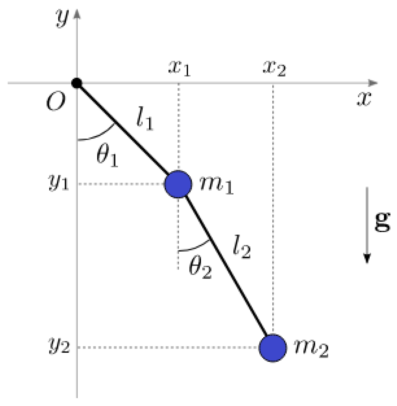
As another example of an underactuated system, consider the double inverted pendulum shown in Figure 2, which is formed by attaching one pendulum directly to another without an actuator between the two links. Each pendulum consists of a mass connected to a massless rigid rod that is constrained to move only within a vertical plane, with the pivot of the first pendulum fixed at point O .
The fixed point O is taken as the origin of the corresponding Cartesian coordinate system, with the x-axis pointing horizontally and the y-axis pointing vertically upward. Let θ 1 and θ 2 denote the angles formed by the first and second rods, respectively, with the vertical axis. Then, the positions of the masses are given by
x 1 = l 1 sin ( θ 1 ) ,
x 2 = l 1 sin ( θ 1 ) + l 2 sin ( θ 2 ) ,
y 1 = l 1 cos ( θ 1 ) ,
y 2 = l 1 cos ( θ 1 ) l 2 cos ( θ 2 ) .
Differentiating the expressions above yields the horizontal and vertical components of the velocities of the corresponding masses, i.e., x ˙ 1 and y ˙ 1 for the first-link velocity v 1 and x ˙ 2 and y ˙ 2 for the second-link velocity v 2 , as follows:
x ˙ 1 = l 1 θ ˙ 1 cos ( θ 1 ) ,
x ˙ 2 = l 1 θ ˙ 1 cos ( θ 1 ) + l 2 θ ˙ 2 cos ( θ 2 ) ,
y ˙ 1 = l 1 θ ˙ 1 sin ( θ 1 ) ,
y ˙ 2 = l 1 θ ˙ 1 sin ( θ 1 ) + l 2 θ ˙ 2 sin ( θ 2 ) .
As with the rotary inverted pendulum, the Lagrangian for the double inverted pendulum is defined by Equation (6), with the difference lying in the expressions for kinetic and potential energy of the first and second links, corresponding to masses m 1 and m 2 , respectively, as follows:
E k = 1 2 m 1 v 1 2 + 1 2 m 2 v 2 2 = 1 2 m 1 x ˙ 1 2 + y ˙ 1 2 + 1 2 m 2 x ˙ 2 2 + y ˙ 2 2 = 1 2 m 1 l 1 2 θ ˙ 1 2 + 1 2 m 2 l 1 2 θ ˙ 1 2 + l 2 2 θ ˙ 2 2 + 2 l 1 l 2 θ ˙ 1 θ ˙ 2 c o s ( θ 1 θ 2 )
E p = m 1 g y 1 + m 2 g y 2 = m 1 g l 1 c o s ( θ 1 ) m 2 g l 1 c o s ( θ 1 ) + l 2 c o s ( θ 2 ) = m 1 + m 2 g l 1 c o s ( θ 1 ) m 2 g l 2 c o s ( θ 2 )
Then, the Lagrangian of the system is given by
L = 1 2 m 1 + m 2 l 1 2 θ ˙ 1 2 + 1 2 m 2 l 2 2 θ ˙ 2 2 + m 2 l 1 l 2 θ ˙ 1 θ ˙ 2 c o s θ 1 θ 2 + m 1 + m 2 g l 1 c o s ( θ 1 ) + m 2 g l 2 c o s ( θ 2 )
Then, according to the Euler–Lagrange equation,
t L q ˙ i L q i = τ i , i = θ 1 , θ 2
we obtain
m 1 + m 2 l 1 θ ¨ 1 + m 2 l 2 θ ¨ 2 c o s θ 1 θ 2 + m 2 l 2 θ ˙ 2 s i n θ 1 θ 2 + m 1 + m 2 g s i n ( θ 1 ) = τ 1 ,
l 2 θ ¨ 2 + l 1 θ ¨ 1 c o s θ 1 θ 2 l 1 θ ˙ 1 2 s i n θ 1 θ 2 + g s i n ( θ 2 ) = τ 2 ,
Evaluating above expressions on equilibrium point where θ 1 = θ 2 0 , θ ˙ 1 = θ ˙ 2 0 , and s i n ( θ i ) θ i for i = 1 , 2 ,
m 1 + m 2 l 1 θ ¨ 1 + m 2 l 2 θ ¨ 2 + m 1 + m 2 g θ 1 = τ 1 ,
l 2 θ ¨ 2 + l 1 θ ¨ 1 + g θ 2 = τ 2 ,
where τ 1 and τ 2 stand for the torque commanded on the first and second link, respectively.
To obtain the following linear state-space model, the system is linearized around the upright equilibrium point θ 1 = 0 , θ 2 = 0 , with zero velocities, since it is desired to stabilize the pendulum in the upright position and to remain fixed on that position. Standard small-angle approximations are applied: sin ( θ i ) θ i and cos ( θ i ) 1 for i = 1 , 2 . These assumptions are valid for small perturbations near the vertical position and are commonly used in control-oriented modeling.
Then, rewriting the above expressions in matrix form and replacing plant parameters such as in [37], with m 1 = 0.4 kgs, m 2 = 0.5 kgs, l 1 = l 2 = 5 mts, and g = 9.8 mts/ sec 2 , we obtain the following state-space representation, with state vector defined as x ( t ) = θ 1 ( t ) θ 2 ( t ) θ ˙ 1 ( t ) θ ˙ 2 ( t ) , as follows:
x ˙ ( t ) = A x ( t ) + B u ( t ) ,
y ( t ) = C x ( t ) + D u ( t ) ,
with
A = 0 0 1 0 0 0 0 1 39.69 24.5 0 0 44.1 49 0 0 ,
B = 0 0 0 0 4.5 2.5 5 5 ,
C = 1 0 0 0 0 1 0 0 0 0 1 0 0 0 0 1 ,
D = 0 .
The derivation of the double inverted pendulum model in this work is based on standard formulations, following the reference in [37]. This model is used solely for simulation-based validation and is not experimentally implemented in a physical setup.

4. Controller Synthesis

4.1. Linear Quadratic Regulator

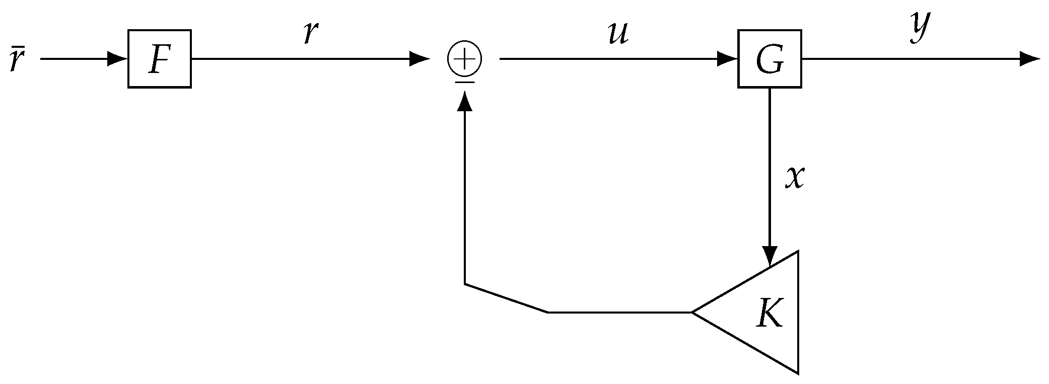
Consider a system described in state-space form with the linear model given by Equations (29) and (30). The Linear Quadratic Regulator (LQR) [4] consists of a state-feedback controller, as illustrated in Figure 3, which defines a cost function to be minimized, as follows:
J = 0 x ( t ) Q x ( t ) + u ( t ) R u ( t ) d t ,
where Q and R are positive semi-definite and positive definite weighting matrices, respectively. The state-feedback control law that minimizes the cost function in Equation (58) is given by
u ( t ) = K x ( t ) ,
where K is defined as
K = R 1 B P ,
and P is the unique positive semi-definite solution to the Algebraic Riccati Equation (ARE), as follows:
A P + P A P B R 1 B P + Q = 0 .

4.2. State-Feedback Controller

The plant G is assumed to follow the form described in Equations (32) and (34). A classical state-feedback control scheme, shown in Figure 3, corresponding to the Linear Quadratic Regulator defined in Equation (59), is considered. The gain matrix K multiplies the plant state x ( t ) to generate the control signal u ( t ) for tracking the reference r ( t ) at time t. In a state-feedback control scheme such as the one in Figure 3, r ( t ) is typically a pre-filtered reference derived from a desired reference r ¯ ( t ) R n y , which represents the target output value y ( t ) at time t, and is mapped into a vector of appropriate dimensions.
A stabilizing controller (with K R n u × n x ) must be designed such that the eigenvalues of A B K lie in the left half-plane in the continuous-time case, or within the unit circle in the discrete-time case [4]. Moreover, to achieve reference tracking—i.e., to ensure that y ( t ) follows r ¯ ( t ) —a pre-filter F (a static gain) is introduced as
F = C A B K I 1 B 1 ,
so that the transfer function from r ¯ ( t ) to y ( t ) is unity.
We now consider a state-feedback control scheme in which the controller has its own internal dynamics, as shown in Figure 4.
Here, the reference vector r ( t ) is assumed to be a pre-filtered version of r ¯ ( t ) , resulting in an n u -dimensional vector representing the desired output components within r ¯ ( t ) . The controller, labeled C o in Figure 4, is assumed to be linear and is described by the following state-space model:
x ˙ c ( t ) = A c x c ( t ) + B c x ( t ) ,
u ( t ) = r ( t ) C c x c ( t ) + D c x ( t ) ,
where the subscript c distinguishes the controller matrices ( A c , B c , C c , D c ) from those of the plant ( A , B , C , D ) , and x c ( t ) represents the controller’s internal state.
Once the controller has been designed, the pre-filter F used to transform r ¯ ( t ) into r ( t ) must be chosen such that the transfer function from r ¯ ( t ) to y ( t ) is unitary to ensure asymptotic tracking. In this case, the static gain F is given by
F = C A I B D c + B C c ( A c I ) 1 B c 1 B 1 .
From Equation (63), we observe that when C c = 0 , the state-feedback law reduces to the simpler static controller shown in Figure 3, with D c equivalent to K. Even in this case, the controller may still have an internal state, though it may not influence the output directly.
Since we are dealing with a dynamic system that includes process and measurement noise, the concept of stability must be extended. Specifically, we focus on Mean Square Stability (MSS) [38]. A system defined by Equations (32) and (34) is said to be mean square stable if and only if there exist μ x R n x and M x R n x × n x , with M x 0 , such that
lim t E { x ( t ) } = μ x ,
lim t E { x ( t ) x ( t ) } = M x .
In practice, an internally unstable controller may still stabilize the control loop, but this is undesirable in real-world applications—especially in robotics—where instability could lead to physical damage.
The controller matrices have dimensions A c R n x c × n x c , B c R n x c × n x , C c R n u × n x c , and D c R n u × n x , where n x c is the dimension of the controller’s internal state x c ( t ) . Note that n x c does not need to be equal to n x .
If we set r ( t ) = 0 for all t and C c = 0 , the problem reduces to a regulation task, where the goal is for x ( t ) 0 as t .
Consider a strictly causal plant as described in Equations (32) and (34) with D = 0 , and a controller defined by Equation (63). Then, the controller stabilizes the system in the mean square sense (as per Equation (66)) if and only if the eigenvalues of the block matrix A ¯ lie in the left half-plane (continuous-time) or within the unit circle (discrete-time), where
A ¯ = A B D c B C c B c A c .
If A ¯ is neither symmetric nor triangular, necessary and sufficient stability conditions cannot be easily obtained from the eigenvalues of its submatrices. However, the eigenvalues of the block matrix A ¯ are given by
eig ( A ¯ ) = eig ( A B D c ) eig ( A c + B c ( A B D c ) 1 B C c ) ,
where, with slight abuse of notation, eig ( X ) denotes the set of dominant eigenvalues of matrix X.
Define the augmented state vector x ¯ ( t ) = x ( t ) x c ( t ) . Then, the augmented system is
x ˙ ¯ ( t ) = A B D c B C c B c A c A ¯ x ¯ ( t ) + B 0 n x c × n u B ¯ r ( t ) + v ( t ) 0 n x c × 1 v ¯ ( t ) ,
where 0 n x c × 1 is a zero column vector of size n x c .
Discretizing the system using a zero-order hold and unit sampling time and unrolling the system in terms of its initial state yields
x ¯ ( t + 1 ) = A ¯ t + 1 x ¯ ( 0 ) + i = 0 t A ¯ i B ¯ r ( t i ) + v ¯ ( t i ) .
Given that v ( t ) is zero-mean white noise, the expectation is
E { x ¯ ( t + 1 ) } = A ¯ t + 1 x ¯ ( 0 ) + i = 0 t A ¯ i B ¯ E { r ( t i ) } .
This is a matrix power series, so to ensure a finite expectation E { x ¯ ( t + 1 ) } as t , it is required that
A ¯ 2 < 1 ,
which, in terms of the dominant eigenvalue, becomes
| eig ( A ¯ ) | < 1 .
A similar analysis for the second-order moment of x ¯ ( t ) leads to the same condition on A ¯ , since the only term contributing to the variance is v ( t ) , which is assumed to have finite variance.
Note that the magnitude of the eigenvalues directly affects the system’s convergence rate: the closer the eigenvalues are to the origin (while remaining within the unit circle), the faster the transient response decays. Conversely, if eigenvalues lie outside the unit circle, the system will exhibit divergent or oscillatory behavior.
Finally, assume for a moment that B c = 0 or C c = 0 . In either case, the controller cannot be internally unstable, and D c must be designed such that A B D c has all eigenvalues within the unit circle. Otherwise, neither the loop nor the controller can be guaranteed to be stable.

4.3. Lyapunov–Based Stability Analysis

In the classical LQR framework, the solution P to the Algebraic Riccati Equation (ARE) in Equation (61) defines a quadratic Lyapunov function V ( x ) = x P x , which certifies asymptotic stability of the closed-loop system when u ( t ) = K x ( t ) and A B K have eigenvalues in the left half-plane.
For the generalized state-feedback controller in Equation (63), the stability condition A ¯ 2 < 1 in Equation (73) ensures Mean Square Stability (MSS) in the presence of zero-mean Gaussian noise. While this is equivalent to a stochastic Lyapunov condition in expectation, direct construction of such a Lyapunov function for the full augmented system remains a complex task and is considered future work.

5. Bayesian Optimization

Bayesian Optimization (BO) [39] is a derivative-free approach for the global optimization of expensive black-box functions f. It belongs to a class of sequential model-based optimization algorithms that use past evaluations of the function to determine the next sampling point.
To understand its necessity, consider a generic maximization problem, as follows:
x * = arg max x X f ( x ) ,
where x * is the global optimizer, and X R m is a bounded domain from which x is selected.
Different variants of Bayesian Optimization employ various acquisition functions to determine the next evaluation point based on the current posterior distribution of the function. The method typically uses Gaussian Processes (GPs) [40] as surrogate models, characterized by a mean function μ ( x ) and a covariance function k ( x , x ) . For n data points, the function values f 1 : n = f ( x 1 ) , , f ( x n ) can be modeled using a multivariate Gaussian distribution, as follows:
f 1 : n N ( μ ( x 1 : n ) , K ) ,
where K is the n × n kernel matrix defined as
K = k ( x 1 , x 1 ) k ( x 1 , x n ) k ( x n , x 1 ) k ( x n , x n ) ,
for a positive-definite kernel such as the Gaussian or Matérn kernel.
An acquisition function determines where to sample next by balancing the trade-off between exploitation and exploration. In this paper, we focus on Expected Improvement (EI) [41].
Expected Improvement evaluates the function at the point where the Expected Improvement over the best observed value f ( x + ) is maximized, given the current GP model, as follows:
E I ( x ) = E [ max { 0 , f ( x ) f ( x + ) ξ } ] = ( μ ( x ) f ( x + ) ξ ) Φ μ ( x ) f ( x + ) ξ σ ( x ) + σ ( x ) ϕ μ ( x ) f ( x + ) ξ σ ( x ) ,
where
-
f ( x + ) is the best function value observed so far;
-
μ ( x ) is the posterior mean at x ;
-
σ ( x ) is the posterior standard deviation;
-
ξ is a small positive parameter encouraging exploration;
-
Φ ( · ) and ϕ ( · ) denote the cumulative distribution function (CDF) and the probability density function (PDF) of the standard normal distribution, respectively.
In our implementation, Bayesian Optimization is used to tune the generalized controller parameters ( A c , B c , C c , D c ) with the goal of minimizing a spectral norm-based cost function Re { eig ( A ¯ ) } , which directly controls the dominant eigenvalue and thus the convergence rate. The optimization is carried out using Gaussian Processes and the Expected Improvement acquisition function. Each function evaluation corresponds to a closed-loop simulation or eigenvalue computation.

6. Simulation Results

In Section 6.1, we first introduce the generalized state-feedback controller in its simplest form, focusing solely on its structure without addressing parameter tuning. This presentation is based on Chapter 3 of [5]. While the aforementioned reference focuses on the rotary inverted pendulum, Section 6.2 and Section 6.3 employ Bayesian Optimization to tune the controller parameters instead of using reinforcement learning as in [5].

6.1. Toy Example

Consider a discrete-time SISO plant (single-input single-output, with n u = 1 and n y = 1 ) given by
x [ k + 1 ] = A x [ k ] + B u [ k ] + v [ k ] ,
y [ k ] = C x [ k ] + w [ k ] ,
where v [ k ] and w [ k ] denote process and measurement noise, respectively—both assumed to be zero-mean white noise with unit variance.
Let A, B, C, and D be defined as
A = 0.5 0 0.7 1.2 ,
B = 0 0.1 ,
C = 1 1 ,
D = 0 .
The plant is internally unstable, as one of its eigenvalues lies outside the unit circle. Therefore, controller parameters A c , B c , C c , and D c must be designed to generate the scalar control signal u [ k ] , as follows:
x c [ k + 1 ] = A c x c [ k ] + B c x [ k ] ,
u [ k ] = r [ k ] C c x c [ k ] + D c x [ k ] ,
with the following matrix values:
A c = 0.4 B c = 1 1.52 , C c = 0.5 D c = 0.3 2.1 .
These values are chosen such that the augmented system matrix A ¯ has prescribed eigenvalues: eig ( A ¯ ) { 0.5 , 0.59 , 0.8 } .
Note from Equation (85) that, in this example, full-state feedback is assumed. The reference is defined as
r [ k ] = 0 if k < 60 , 10 if k 60 .
We compare this control scheme to the classical state-feedback architecture shown in Figure 3, where the output is y [ k ] and the control signal is
u [ k ] = r [ k ] K x [ k ] ,
with gain matrix, as follows:
K = 0.3 4 ,
chosen so that eig ( A B K ) { 0.5 , 0.8 } .
As expected from the eigenvalue analysis of A ¯ and A B K , the closed-loop system reaches stationarity at the same rate (defined by the dominant eigenvalue, which governs the slowest decaying mode). However, D c and K differ, because the generalized controller in Figure 4 introduces additional degrees of freedom compared with the classical scheme in Figure 3, at the cost of adding an extra natural mode to the closed-loop response.
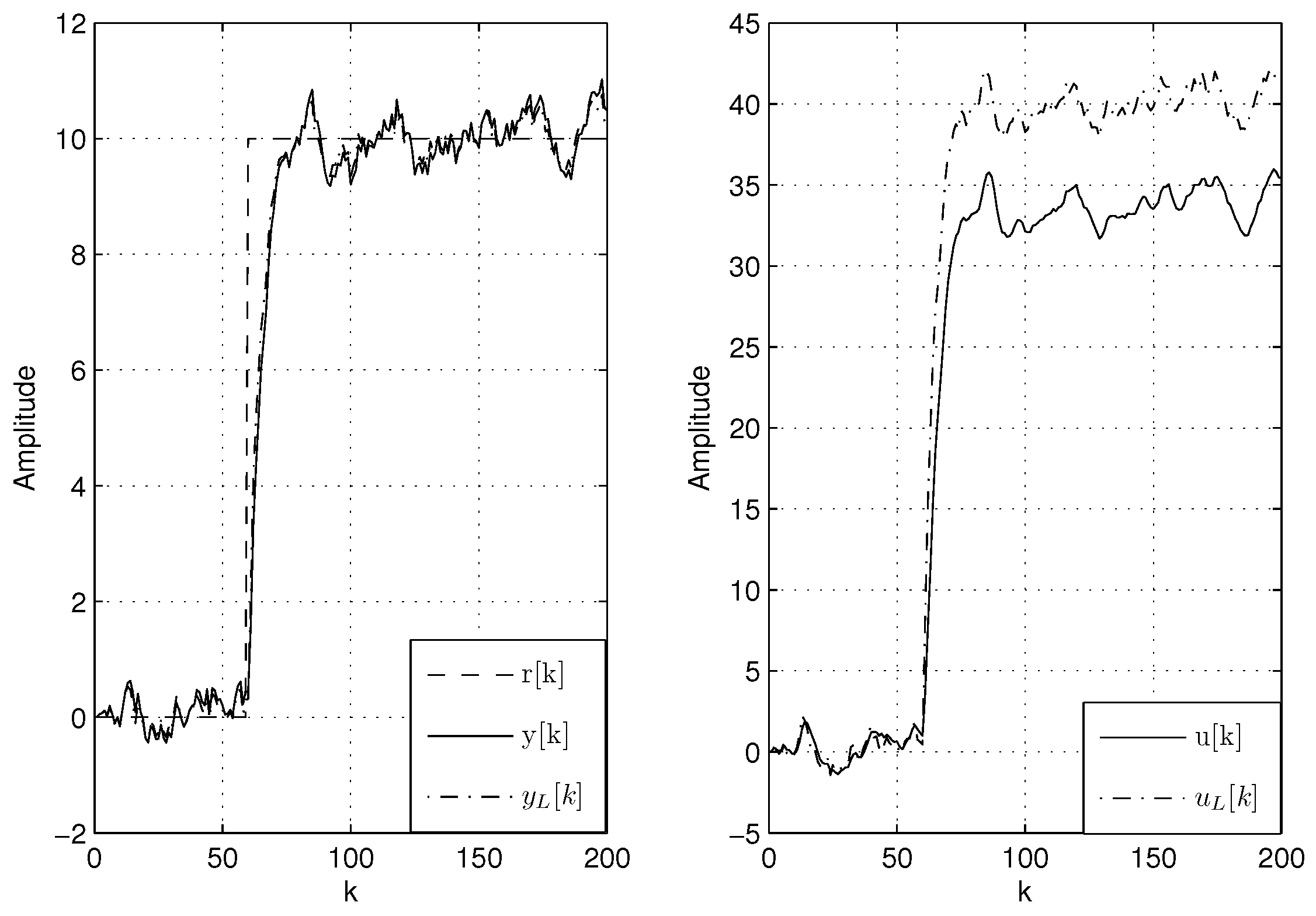
Simulation results in Figure 5 show that the additional degrees of freedom allow tuning the controller such that stationarity is achieved at the same rate while producing a smaller control signal than in the classical case.
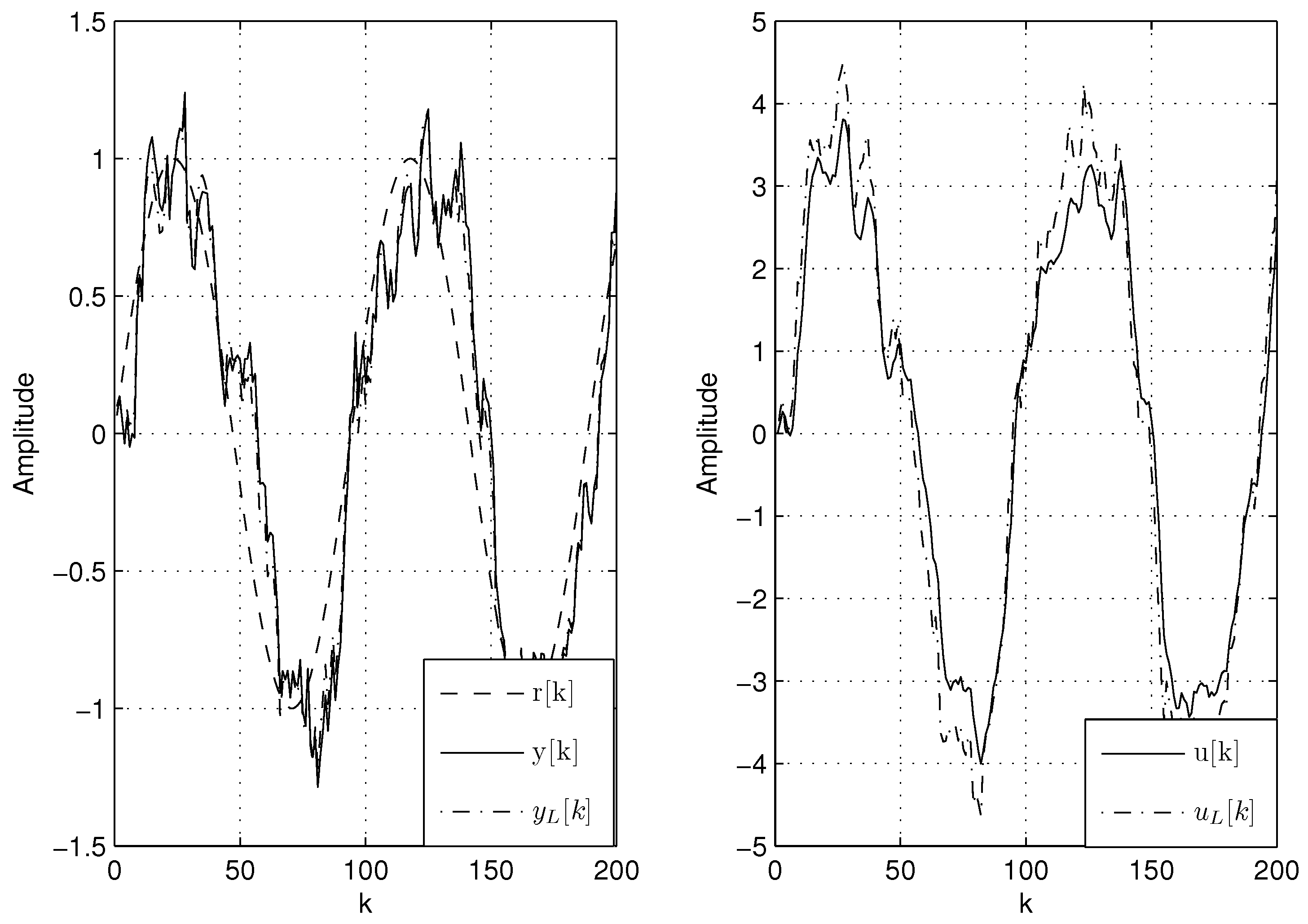
Figure 6 presents the same comparison using a sinusoidal reference. Results confirm the previous observation: both controllers yield the same convergence speed, but the dynamic controller results in lower control signal peaks due to its additional degrees of freedom. Note, however, that tracking is only achievable if the closed-loop dynamics are sufficiently fast to follow changes in the reference.

6.2. Experimental Results: Rotary Inverted Pendulum

When considering the parameters from Table 1 for the model described in Equations (32) and (34), the following matrices are obtained:
A = 0 1 0 0 0 0 0.31 2.99 0.02 81.47 0 0 0 1 0 0 0.02 61.49 0.5 63.88 0 261.94 0 0 800 ,
B = 0 0 0 0 100 ,
C = 1 0 0 0 0 0 0 1 0 0 0 0 0 0 1 .
The performance of the proposed controller in Equation (63) for the rotary inverted pendulum is compared against the classical state-feedback controller defined in Equation (59). To this end, matrices Q and R from Equation (58) are designed to assign more weight to states that are more relevant to the specific experiment. In this case, priority is given to the pendulum position θ 1 , while arm and pendulum velocities are also considered important. The chosen matrices are
Q = 1 0 0 0 0 0 10 0 0 0 0 0 100 0 0 0 0 0 10 0 0 0 0 0 1 ,
R = 10 ,
where the penalty matrix R is selected to avoid sudden changes in the control signal that could destabilize the pendulum due to the DC motor’s behavior.
Solving Equation (61) with the model in Equation (89) yields
K = 0.31 5.26 70.74 8.92 0.17 .
Alternatively, for controllers of the form given in Equation (63), parameters are obtained by applying Bayesian Optimization with a maximum of 150 iterations, minimizing
Re { eig ( A ¯ ) } ,
where A ¯ is the closed-loop matrix defined in Equation (68), and Re { eig ( M ) } denotes the real parts of the eigenvalues of matrix M. The minimization of the infinity norm constrains the maximum eigenvalue, thus limiting the dominant system response speed. This yields
A c = 100 ,
B c = 0 0 0 0 0 ,
C c = 0.5 ,
D c = 20.96 39.76 72.74 92.61 0.58 .
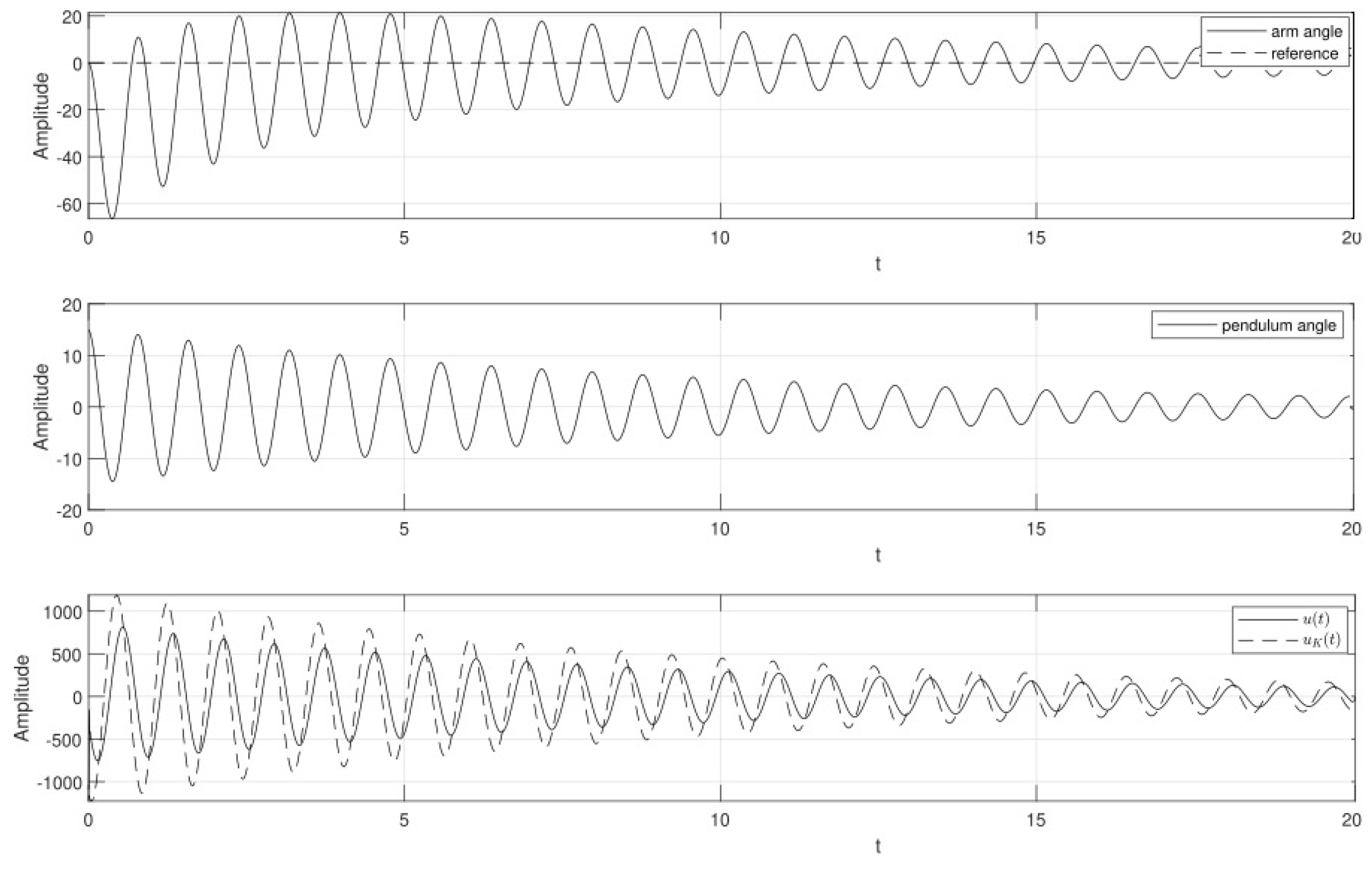
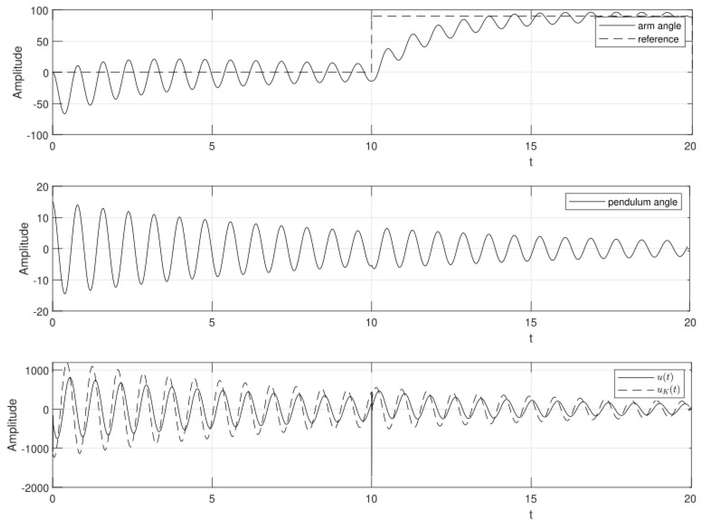
Figure 7 shows the arm and pendulum positions in the upper and middle subplots, respectively. It can be observed that both controllers successfully stabilize the pendulum while controlling the arm position. The lower subplot confirms the same behavior seen in Figure 6, where the controller in Equation (63) achieves similar performance to the LQR controller in Equation (59), but with reduced control effort. Figure 8 further illustrates this when the arm reference is changed while maintaining pendulum stabilization.
Although not shown with additional figures, the simulations included variations in reference signals (through step functions) and initial conditions. The controller consistently achieved stable regulation and reference tracking, demonstrating robustness and effective performance across different dynamic scenarios.
It is important to note that Bayesian Optimization is not used to compute the conventional K gain in Figure 3, which can be derived via ARE. Instead, Bayesian Optimization tunes the parameters of the generalized dynamic controller in Figure 4, enabling improved performance (e.g., lower control energy) not achievable by LQR alone.
The code for obtention of results for this section is available at https://github.com/miguel-a-solis/MDPI_Mathematics_SI-2025 (accessed on 1 August 2025).

6.3. Double Inverted Pendulum

Based on the model from Equation (54), the matrices Q and R in Equation (58) are defined to prioritize the pendulum position over the first-link position, which is less relevant in this case. The matrices are
Q = 1 0 0 0 0 10 0 0 0 0 100 0 0 0 0 10 .
R = 10 ,
Solving Equation (61) yields the LQR gain, as follows:
K = 6.95 0.06 0.03 2.21 .
By minimizing the infinity norm of the real parts of the closed-loop eigenvalues as described in Equation (95), the following controller parameters are obtained:
A c = 1.29 ,
B c = 0 0 0 0 ,
C c = 0.5 ,
D c = 60.01 22.84 0.53 94.06 .
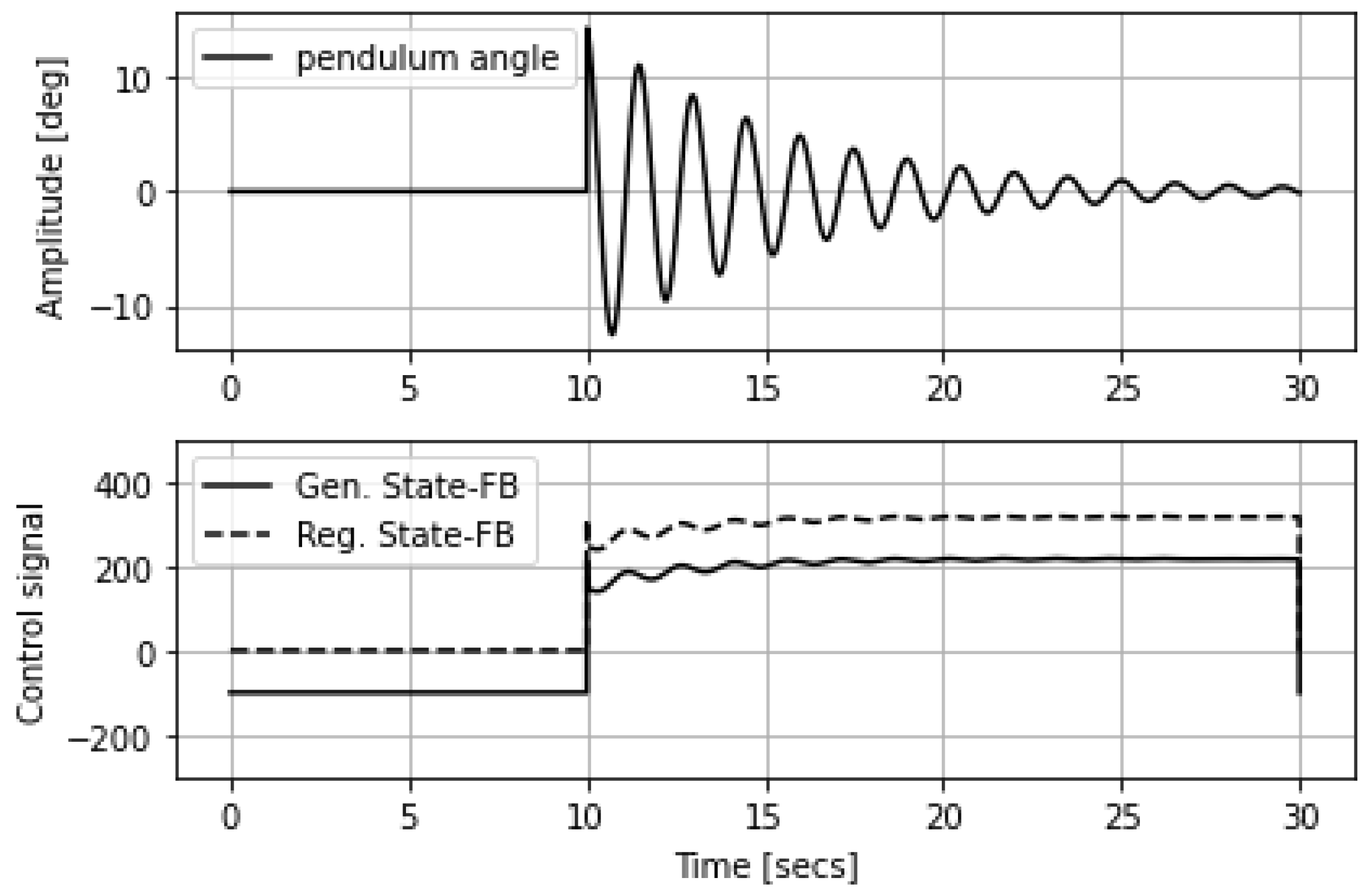
Figure 9 shows the pendulum position (top subplot) and control signal (bottom subplot). Both controllers stabilize the pendulum effectively; however, the generalized state-feedback controller achieves this with a lower-amplitude control signal, which corresponds to a reduced voltage demand on the motor.
The proposed controller was tested under different operating points and state configurations. Despite the structural differences between the rotary inverted pendulum and double inverted pendulum systems, the generalized controller maintained comparable performance with the LQR approach, while reducing control effort. This highlights its adaptability and potential applicability to a broader class of underactuated systems.

6.4. Numerical Performance

The following Table 2 summarizes key performance indices for each control scenario, including the settling time, maximum overshoot, and Integral Square Error (ISE), which reflects the cumulative deviation from the desired output, as follows:
The generalized controller shows reasonably fast convergence, limited overshoot, and bounded control effort, even under large reference changes. The inclusion of ISE complements this analysis by quantifying the overall tracking accuracy and disturbance rejection.
Beyond the settling time and overshoot metrics, the Integral of Squared Error (ISE) provides an additional perspective on the control performance. In the double inverted pendulum scenario, the ISE remains within acceptable bounds given the system’s high instability and extended transient phase. For the Furuta pendulum with step reference, the controller achieves fast convergence and low ISE, indicating precise tracking with minimal sustained error. In contrast, the constant reference case exhibits a higher ISE, mainly due to the sharp change in the reference signal that induces a brief but significant transient error. Nevertheless, the system stabilizes quickly, and no long-term oscillations are observed. These results confirm that the controller tuned via Bayesian Optimization offers reliable performance across diverse conditions, balancing transient accuracy with stability, even under nonlinear and underactuated dynamics.
Although the proposed approach demonstrates promising results, one limitation lies in the practical implementation of full-state feedback controllers. In real-world scenarios, not all state variables are directly measurable or observable, especially in underactuated systems where sensing is limited due to cost, hardware constraints, or noise susceptibility. As discussed in [42], full-state feedback often assumes ideal access to all state variables, which is rarely the case. Instead, output-feedback or observer-based designs are commonly used in practice [43], which introduces additional challenges such as robustness to estimation errors and increased computational complexity.
Therefore, while the generalized controller proposed in this article provides a flexible structure for performance improvement, future work should address its integration with state estimators or reduced-order observers to enhance its applicability in practical control systems.

7. Conclusions

This work has presented a Bayesian Optimization approach for tuning a generalized state-feedback controller and compared its performance against the classical controller obtained by solving the Linear Quadratic Regulator (LQR) problem. Simulation results demonstrated that the proposed control scheme achieves the same tracking performance as the classical one, but with reduced control effort.
In addition, a well-known underactuated system—the rotary inverted pendulum (also known as the Furuta pendulum)—was studied, and a corresponding linear model was derived. Simulations were conducted using this plant model, and once again, the generalized controller exhibited tracking performance comparable to that of the classical state-feedback controller, while requiring lower control signal amplitudes. In contrast with the rotary inverted pendulum, on the double inverted pendulum, all results were obtained in a simulated environment, where implementation on a physical prototype is left as future work.
It is important to note that our methodology assumes full state availability, which may not be realistic in many practical systems. For instance, the second state on the observation matrix for the rotary inverted pendulum is typically not directly measurable. There is literature on observer-based control, such as proportional-integral observers for wind energy systems and attack-tolerant observers in cyber-physical systems, that provides promising alternatives to reconstruct unmeasured states. Future work will explore integrating such observer architectures into the Bayesian tuning process.

Author Contributions

Conceptualization, M.A.S. and S.S.T.; methodology, M.A.S. and S.S.T.; software, M.A.S., C.A.C.-S. and E.A.T.-A.; validation, M.A.S., S.S.T. and E.A.T.-A.; formal analysis, M.A.S.; investigation, M.A.S. and S.S.T.; resources, M.A.S.; data curation, M.A.S.; writing—original draft preparation, M.A.S.; writing—review and editing, F.C.; visualization, M.A.S.; supervision, S.S.T.; project administration, S.S.T.; funding acquisition, S.S.T. All authors have read and agreed to the published version of the manuscript.

Funding

The APC was funded by Universidad Nacional Jorge Basadre Grohmann.

Data Availability Statement

The original data presented in this study are openly available in GitHub at https://github.com/miguel-a-solis/MDPI_Mathematics_SI-2025 accessed on 1 August 2025.

Conflicts of Interest

The authors declare no conflicts of interest.

Abbreviations

The following abbreviations are used in this manuscript:
AREAlgebraic Riccati Equation
BOBayesian Optimization
CDFcumulative distribution function
DCdirect current
DIPdouble inverted pendulum
EIExpected Improvement
GPGaussian Process
ISEIntegral Square Error
LQRLinear Quadratic Regulator
PDFprobability density function
RIProtary inverted pendulum
SISO             Single Input Single Output
Summary of key symbols, definitions, and units used throughout the manuscript.
SymbolDescriptionUnits
x ( t ) State vector of the plant
x c ( t ) State vector for the controller
u ( t ) Control input signalVolts (V)
y ( t ) Output measurement
r ( t ) Filtered reference signal
r ¯ ( t ) Desired reference trajectory
A , B , C , D      State-space matrices of the plant                                         
A c , B c , C c , D c Controller state-space matrices
KFeedback gain matrix (static controller)
FPre-filter gain matrix
PSolution to the Algebraic Riccati Equation
Q , R LQR weighting matrices
A ¯ Augmented closed-loop system matrix
A ¯ 2 Spectral norm (largest singular value)
eig ( · ) Eigenvalues of a matrix
v ( t ) , w ( t ) Process and measurement zero-mean noiseGaussian
P v , P w Covariance matrices for v ( t ) and w ( t )
JCost function
V ( x ) Lyapunov function
μ ( x ) Posterior mean of surrogate function (BO)
σ ( x ) Posterior standard deviation (BO)
ξ Exploration parameter in acquisition function
Φ ( · ) , φ ( · ) Standard Gaussian CDF and PDF
θ 0 , θ 1 Arm and pendulum angles (Rotary Inverted Pendulum)radians
θ ˙ i , θ ¨ i Angular velocity and accelerationrad/s, rad/s2
M 1 , M 2 , M 3 Inertia, Coriolis and gravity matrices
τ Applied torqueNm
i ( t ) Motor currentA
V ( t ) Motor voltage inputV
ω , ω e Angular velocitiesrad/s
K g , K e g Gear ratios
M f Motor torque constantNm/A
R a , L a Armature resistance and inductance Ω , H
N ( 0 , P ) Normal distribution with zero mean and covariance P

References

  1. Olfati-Saber, R. Nonlinear Control of Underactuated Mechanical Systems with Application to Robotics and Aerospace Vehicles. Ph.D. Thesis, Massachusetts Institute of Technology, Cambridge, MA, USA, 2001. [Google Scholar]
  2. Spong, M.W. Underactuated mechanical systems. In Control Problems in Robotics and Automation; Springer: Berlin/Heidelberg, Germany, 2005; pp. 135–150. [Google Scholar]
  3. Birglen, L.; Laliberté, T.; Gosselin, C.M. Underactuated Robotic Hands; Springer: Berlin/Heidelberg, Germany, 2007; Volume 40. [Google Scholar]
  4. Anderson, B.D.; Moore, J.B. Optimal Control: Linear Quadratic Methods; Courier Corporation: North Chelmsford, MA, USA, 2007. [Google Scholar]
  5. Solís Cid, M.A. Reinforcement Learning on Control Systems with Unobserved States. Ph.D. Thesis, Universidad Técnica Federico Santa María, Valparaíso, Chile, 2017. [Google Scholar]
  6. Yu, H.; Liu, Y.; Yang, T. Closed-loop Tracking Control of a Pendulum-driven Cart-pole Underactuated System. Proc. Inst. Mech. Eng. Part I J. Syst. Control. Eng. 2008, 222, 109–125. [Google Scholar] [CrossRef]
  7. Åström, K.J.; Furuta, K. Swinging up a Pendulum by Energy Control. Automatica 2000, 36, 287–295. [Google Scholar] [CrossRef]
  8. Cui, Z.; Zeng, J.; Sun, G. A fast particle swarm optimization. Int. J. Innov. Comput. Inf. Control. 2006, 2, 1365–1380. [Google Scholar]
  9. Kong, L.; He, W.; Dong, Y.; Cheng, L.; Yang, C.; Li, Z. Asymmetric Bounded Neural Control for an Uncertain Robot by State Feedback and Output Feedback. IEEE Trans. Syst. Man Cybern. Syst. 2021, 51, 1735–1746. [Google Scholar] [CrossRef]
  10. Sutton, R.S.; Barto, A.G. Reinforcement Learning: An Introduction; MIT Press: Cambridge, MA, USA, 2018. [Google Scholar]
  11. Barbieri, E.; Alba-Flores, R. On the Infinite-horizon LQ tracker. Syst. Control. Lett. 2000, 40, 77–82. [Google Scholar] [CrossRef]
  12. Qin, C.; Zhang, H.; Luo, Y. Online Optimal Tracking Control of Continuous-time Linear Systems with Unknown Dynamics by using Adaptive Dynamic Programming. Int. J. Control. 2014, 87, 1000–1009. [Google Scholar] [CrossRef]
  13. Kiumarsi, B.; Lewis, F.L.; Modares, H.; Karimpour, A.; Naghibi-Sistani, M.B. Reinforcement Q-learning for optimal tracking control of linear discrete-time systems with unknown dynamics. Automatica 2014, 50, 1167–1175. [Google Scholar] [CrossRef]
  14. Watkins, C.J.; Dayan, P. Q-learning. Mach. Learn. 1992, 8, 279–292. [Google Scholar] [CrossRef]
  15. Kumar, Y.P.; Pradeep, D.J.; Chakravarthi, M.K.; Reddy, G.P. Deep Learning-Based PID Controller Tuning for Effective Speed Control of DC Shunt Motors. In Proceedings of the 2025 IEEE Open Conference of Electrical, Electronic and Information Sciences (eStream), Vilnius, Lithuania, 24 April 2025; pp. 1–6. [Google Scholar]
  16. Saat, S.; Ahmad, M.A.; Ghazali, M.R. Data-driven brain emotional learning-based intelligent controller-PID control of MIMO systems based on a modified safe experimentation dynamics algorithm. Int. J. Cogn. Comput. Eng. 2025, 6, 74–99. [Google Scholar] [CrossRef]
  17. Suid, M.H.; Ahmad, M.A. Optimal tuning of sigmoid PID controller using nonlinear sine cosine algorithm for the automatic voltage regulator system. ISA Trans. 2022, 128, 265–286. [Google Scholar] [CrossRef] [PubMed]
  18. Aoki, M. On some convergence questions in bayesian optimization problems. IEEE Trans. Autom. Control. 1965, 10, 180–182. [Google Scholar] [CrossRef]
  19. Poloczek, M.; Wang, J.; Frazier, P. Multi-Information Source Optimization. In Proceedings of the Advances in Neural Information Processing Systems, Long Beach, CA, USA, 4–9 December 2017; Volume 30, pp. 4288–4298. [Google Scholar]
  20. Ghoreishi, S.F.; Imani, M. Bayesian Optimization for Efficient Design of Uncertain Coupled Multidisciplinary Systems. In Proceedings of the 2020 American Control Conference (ACC), Denver, CO, USA, 1–3 July 2020; pp. 3412–3418. [Google Scholar]
  21. Baptista, R.; Poloczek, M. Bayesian Optimization of Combinatorial Structures. In Proceedings of the International Conference on Machine Learning, Stockholm, Sweden, 10–15 July 2018; pp. 462–471. [Google Scholar]
  22. Nguyen, V.; Gupta, S.; Rana, S.; Li, C.; Venkatesh, S. Regret for Expected Improvement over the Best-Observed Value and Stopping Condition. In Proceedings of the 9th Asian Conference on Machine Learning, Seoul, Republic of Korea, 15–17 November 2017; Volume 77, pp. 279–294. [Google Scholar]
  23. Snoek, J.; Larochelle, H.; Adams, R.P. Practical Bayesian Optimization of Machine Learning Algorithms. In Proceedings of the Advances in Neural Information Processing Systems, Lake Tahoe, NV, USA, 3–6 December 2012; pp. 2951–2959. [Google Scholar]
  24. Lyu, W.; Xue, P.; Yang, F.; Yan, C.; Hong, Z.; Zeng, X.; Zhou, D. An Efficient Bayesian Optimization Approach for Automated Optimization of Analog Circuits. IEEE Trans. Circuits Syst. I Regul. Pap. 2017, 65, 1954–1967. [Google Scholar] [CrossRef]
  25. Hu, H.; Li, P.; Huang, J.Z. Enabling High-Dimensional Bayesian Optimization for Efficient Failure Detection of Analog and Mixed-Signal Circuits. In Proceedings of the ACM 56th Annual Design Automation Conference 2019, Las Vegas, NV, USA, 2–6 June 2019; pp. 17:1–17:6. [Google Scholar]
  26. Lam, R.; Poloczek, M.; Frazier, P.; Willcox, K.E. Advances in Bayesian Optimization with Applications in Aerospace Engineering. In Proceedings of the AIAA Non-Deterministic Approaches Conference, Kissimmee, FL, USA, 8–12 January 2018; p. 1656. [Google Scholar]
  27. Sano, S.; Kadowaki, T.; Tsuda, K.; Kimura, S. Application of Bayesian optimization for pharmaceutical product development. J. Pharm. Innov. 2020, 15, 333–343. [Google Scholar] [CrossRef]
  28. Kocijan, J.; Grancharova, A. Application of Gaussian processes to the modelling and control in process engineering. In Innovations in Intelligent Machines-5; Springer: Berlin/Heidelberg, Germany, 2014; pp. 155–190. [Google Scholar]
  29. Wang, H.; Xu, H.; Yuan, Y.; Deng, J.; Sun, X. Noisy Multiobjective Black-box Optimization Using Bayesian Optimization. In Proceedings of the Genetic and Evolutionary Computation Conference Companion, Prague, Czech Republic, 13–17 July 2019; GECCO ’19. pp. 239–240. [Google Scholar]
  30. Kirschner, J.; Mutny, M.; Hiller, N.; Ischebeck, R.; Krause, A. Adaptive and Safe Bayesian Optimization in High Dimensions via One-Dimensional Subspaces. In Proceedings of the 36th International Conference on Machine Learning, Long Beach, CA, USA, 9–15 June 2019; Volume 97, pp. 3429–3438. [Google Scholar]
  31. Zhang, Y.; Liu, L.; Liang, J.; Chen, J.; Ke, C.; He, D. Application of a multi-strategy improved sparrow search algorithm in bridge crane PID control systems. Appl. Sci. 2024, 14, 5165. [Google Scholar] [CrossRef]
  32. Nasir, N.M.; Ghani, N.M.A.; Nasir, A.N.K.; Ahmad, M.A.; Tokhi, M.O. Neuro-modelling and fuzzy logic control of a two-wheeled wheelchair system. J. Low Freq. Noise Vib. Act. Control. 2025, 44, 588–602. [Google Scholar] [CrossRef]
  33. Imani, M.; Ghoreishi, S.F. Bayesian optimization objective-based experimental design. In Proceedings of the 2020 American control conference (ACC), Denver, CO, USA, 1–3 July 2020; pp. 3405–3411. [Google Scholar]
  34. Wang, X.; Jin, Y.; Schmitt, S.; Olhofer, M. Recent advances in Bayesian optimization. ACM Comput. Surv. 2023, 55, 1–36. [Google Scholar] [CrossRef]
  35. Solis, M.A.; Olivares, M.; Allende, H. A Switched Control Strategy for Swing-up and State Regulation for the Rotary Inverted Pendulum. Stud. Informatics Control. 2019, 28, 45–54. [Google Scholar] [CrossRef]
  36. Friedland, B. Control System Design: An Introduction to State-Space Methods; Courier Corporation: North Chelmsford, MA, USA, 2012. [Google Scholar]
  37. Crowe-Wright, I.J. Control Theory: The Double Pendulum Inverted on a Cart. Bachelor’s Thesis, University of New Mexico, Albuquerque, NM, USA, 2018. [Google Scholar]
  38. Willems, J. Mean Square Stability Criteria for Stochastic Feedback Systems. Int. J. Syst. Sci. 1973, 4, 545–564. [Google Scholar] [CrossRef]
  39. Thomas, S.S.; Palandri, J.; Lakehal-Ayat, M.; Chakravarty, P.; Wolf-Monheim, F.; Blaschko, M.B. Designing MacPherson Suspension Architectures Using Bayesian Optimization. In Proceedings of the 31st Benelux Conference on Artificial Intelligence (BNAIC 2019) and the 28th Belgian Dutch Conference on Machine Learning (Benelearn 2019), Brussels, Belgium, 6–8 November 2019. [Google Scholar]
  40. Rasmussen, C.E.; Williams, C.K.I. Gaussian Processes for Machine Learning; MIT Press: Cambridge, MA, USA, 2005. [Google Scholar]
  41. Brochu, E.; Cora, V.M.; De Freitas, N. A Tutorial on Bayesian Optimization of Expensive Cost Functions, with Application to Active User Modeling and Hierarchical Reinforcement Learning. Technical Report. 2010. Available online: https://ora.ox.ac.uk/objects/uuid:9e6c9666-5641-4924-b9e7-4b768a96f50b (accessed on 1 August 2025).
  42. Franklin, G.F.; Powell, J.D.; Emami-Naeini, A.; Powell, J.D. Feedback Control of Dynamic Systems; Pearson: Upper Saddle River, NJ, USA, 2010; Volume 10. [Google Scholar]
  43. Khalil, H.K.; Grizzle, J.W. Nonlinear Systems; Prentice Hall: Upper Saddle River, NJ, USA, 2002; Volume 3. [Google Scholar]
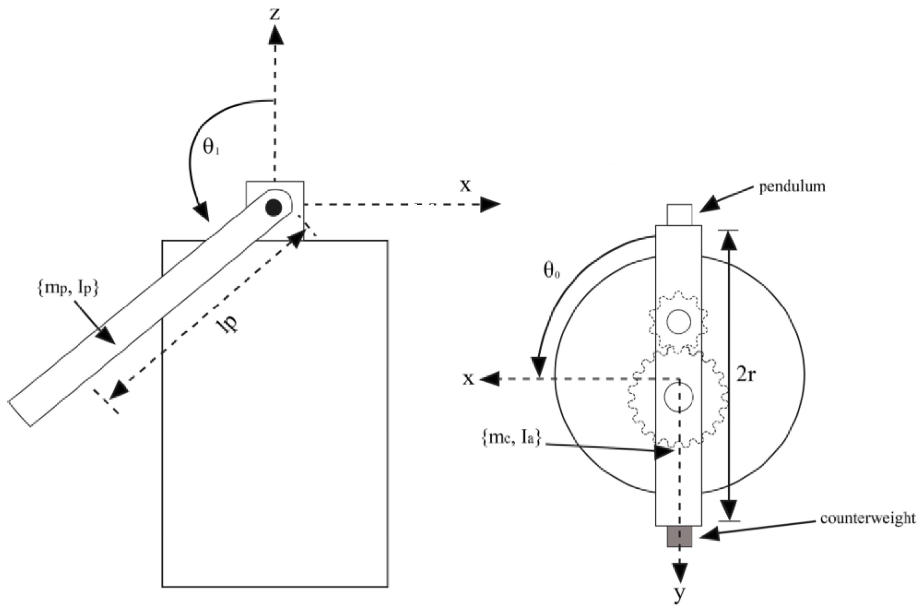
Figure 1. Side and top views of the Furuta pendulum.
Mathematics 13 03139 g001
Figure 2. Side view of the Double Inverted Pendulum.
Mathematics 13 03139 g002
Figure 3. Classical state-feedback control scheme for plant G and controller (gain) K.
Mathematics 13 03139 g003
Figure 4. Dynamical state-feedback control proposed scheme for plant G and controller C o .
Mathematics 13 03139 g004
Figure 5. Full state-feedback: step reference tracking.
Mathematics 13 03139 g005
Figure 6. Full state-feedback: sinusoidal reference tracking.
Mathematics 13 03139 g006
Figure 7. Furuta pendulum control.
Mathematics 13 03139 g007
Figure 8. Furuta pendulum control with reference tracking for arm angle.
Mathematics 13 03139 g008
Figure 9. Double inverted pendulum control.
Mathematics 13 03139 g009
Table 1. RIP parameters.
SymbolDescriptionValue
m p Pendulum mass 0.1 kg
m c Counterweight mass 0.01 kg
I p Pendulum inertial moment 5.1 × 10 4 kg m 2
I a Arm inertial moment 3.1 × 10 3 kg m 2
rArm radius 0.13 m
l p Pendulum mass center 0.125 m
hArm center of mass height 0.055 m
C 0 Arm friction coefficient 10 4
C 1 Pendulum friction coefficient 10 4
R a Armature resistor8 Ω
L a Motor inductance10 mH
I m Motor inertia 1.9 × 10 6 kg m 2
M f Motor mutual inductance 0.0214 N m/A
K g Gear reduction coefficient59,927
K e g External gear reduction coefficient16
gGravitational acceleration 9.806 m/ s 2
Table 2. Numerical performance indices on different scenarios.
SystemSettling Time (s)Max Overshoot (°)ISE
Double Inverted Pendulum (BO)∼1813.543.1
Furuta (Step Reference, BO)∼610.0170.2
Furuta (Constant Reference, BO)∼940.0129.7
Disclaimer/Publisher’s Note: The statements, opinions and data contained in all publications are solely those of the individual author(s) and contributor(s) and not of MDPI and/or the editor(s). MDPI and/or the editor(s) disclaim responsibility for any injury to people or property resulting from any ideas, methods, instructions or products referred to in the content.