Abstract
The fatigue constitutive model under cyclic loading is of vital importance for studying the fatigue deformation characteristics of soft rocks. In this paper, based on the classical Bingham model, a modified Bingham fatigue model for describing the fatigue deformation characteristics of soft rocks under cyclic loading was developed. Firstly, the traditional constant-viscosity component was replaced by an improved nonlinear viscoelastic component related to the number of cycles. The elastic component was replaced by an improved nonlinear elastic component that decays as the number of cycle loads increases. Meanwhile, by decomposing the cyclic dynamic loads into static loads and alternating loads, a one-dimensional nonlinear viscoelastic-plastic Bingham fatigue model was developed. Furthermore, a rock fatigue yield criterion was proposed, and by using an associated flow rule compatible with this criterion, the one-dimensional fatigue model was extended to a three-dimensional constitutive formulation under complex stress conditions. Finally, the applicability of the developed Bingham fatigue model was verified through fitting with experimental data, and the parameters of the model were identified. The model fitting results show high consistency with experimental data, with correlation coefficients exceeding 0.978 and 0.989 under low and high dynamic stress conditions, respectively, and root mean square errors (RMSEs) below 0.028. Comparative analysis between theoretical predictions and existing soft rock fatigue test data demonstrates that the developed Bingham fatigue model more effectively captures the complete fatigue deformation process under cyclic loading, including the deceleration, constant velocity, and acceleration phases. With its simplified component configuration and straightforward combination rules, this model provides a valuable reference for studying fatigue deformation characteristics of rock materials under dynamic loading conditions.
Keywords:
rock mechanics; cyclic loading; nonlinear; visco-elasto-plastic; Bingham model; fatigue constitutive model MSC:
37M10
1. Introduction
The fatigue deformation process of rock materials is of vital importance to the stability of engineering construction. In geotechnical engineering projects such as water conservancy and hydropower, deep mining, transportation tunnels, and submarine construction, fatigue issues frequently impact the safety of structures and the stability of bedrock. For instance, the impact of periodic water level fluctuations on dams, the influence of cyclic dynamic loads from deep mining on surrounding rock, the effect of cyclic traffic loads on bedrock, and the cyclic load from wave effects on the underwater geological strata. Under long-term cyclic loading, rock strength degrades progressively, potentially leading to fatigue failure and engineering accidents. Soft rock, a highly plastic rock medium formed under specific geological conditions, represents a specialized material category. Recent decades have witnessed increasing utilization of soft rock in infrastructure projects, including roadbeds, tunnels, and submarine geological layers. Given its complex engineering mechanical behavior, the study of fatigue deformation characteristics in soft rock under cyclic loading holds significant theoretical importance for evaluating long-term rock mass stability and optimizing engineering designs.
The study of constitutive models for soft rock under cyclic loading has emerged as a research hotspot and challenge in recent years [1,2,3,4]. However, limited research has been conducted on fatigue constitutive models specifically tailored for soft rock. Existing constitutive frameworks in this domain can be categorized into four primary categories: Empirical constitutive models based on experimental data fitting [5,6,7], Damage constitutive models grounded in continuum damage mechanics [2,8,9], Energy-based constitutive models incorporating thermodynamic principles [10,11], and Component-based constitutive models integrating rheological elements [12,13,14]. Given that the component combination model based on rheological theory has the advantages of clear physical meaning and relatively intuitive concepts; therefore, constructing and improving the component combination model is a common method for scholars to establish the fatigue constitutive model of soft rock under cyclic loading. The traditional rheological component model is limited to describing the first two stages of rheological behavior, namely the deceleration and constant velocity stages. However, many researchers believe that there is an acceleration stage before the rock rheological failure, which is difficult for the traditional model to fully represent [15,16].
Therefore, many scholars have proposed nonlinear rheological models [17,18,19,20], which can describe the third stage of rheology, namely the acceleration stage. Furthermore, Mo [21] conducted cyclic loading tests on red sandstone and marble to derive the internal time-dependent constitutive equation for rocks. However, the equation contains numerous parameters, including 5 parameters, and lacks clear physical significance. Wang et al. [22] established the constitutive equation for rocks under cyclic confining pressure loading based on the Burgers model, but the model is only applicable under the condition of low-frequency cyclic loading. Guo et al. [23] proposed three basic elements of fatigue: elastic fatigue component, viscous fatigue component and plastic fatigue component, and established a viscoelastic-plastic rock fatigue constitutive model under uniaxial cyclic loading. Later, Wang et al. [24] replaced the conventional viscous elements in the Maxwell model with nonlinear viscous elements, thereby establishing an improved Maxwell model that can describe the entire process of salt rock creep. Rezaiee-Pajand et al. [25,26] developed a MITC-based 4-node curved beam element for thermo-mechanical nonlinear analysis of FGM structures, achieving shear-locking-free performance with three Gauss integration points while accurately modeling large deformation and rotation through Total-Lagrangian formulation. In recent years, Li et al. [27] developed an improved viscoplastic model based on fractional calculus, which can effectively capture the complete creep evolution process under the influence of thermal-thermal coupling interference. Cai et al. [28] developed a fractional-order viscoelastic model with physical interpretability and high parameter efficiency, which can accurately capture the nonlinear accelerated creep behavior, thus providing a practical framework for predicting the creep behavior of viscoelastic materials.
Current research indicates a scarcity of constitutive models for soft rock under cyclic loading. Existing approaches often oversimplify dynamic loads as static forces by directly imposing cyclic loads onto models. Consequently, developed models essentially remain static constitutive or static empirical constitutive frameworks, characterized by excessive parameters and complex component configurations. However, soft rock exhibits substantially larger strains than hard rocks under cyclic loading, with its oscillatory response being non-negligible. Most importantly, no generalizable fatigue constitutive model currently exists for soft rock deformation under periodic loading. Therefore, in this paper, based on the principle of rheology, the classical Bingham model was modified, and an improved Bingham fatigue model for describing the fatigue deformation characteristics of soft rocks under cyclic loading was developed. Firstly, the traditional constant-viscosity component was replaced by an improved nonlinear viscoelastic component related to the number of cycles. The elastic component was replaced by an improved nonlinear elastic component that decays as the number of cycle loads increases. Meanwhile, by decomposing the cyclic dynamic loads into static loads and alternating loads, a one-dimensional nonlinear viscoelastic-plastic Bingham fatigue model was developed. Furthermore, a rock fatigue yield criterion was proposed, and by using an associated flow rule compatible with this criterion, the one-dimensional fatigue model was extended to a three-dimensional constitutive formulation under complex stress conditions. Finally, the applicability of the developed Bingham fatigue model was verified through fitting with experimental data, and the parameters of the model were identified. The combined form of the model developed in this paper is simple, the proposed theory is easy to understand, and the parameters have clear physical meanings. The research results not only enrich the theory of rock rheology, but can also be applied to slopes, tunnels and water conservancy projects.
2. Fundamental Theory of Soft Rock Deformation Under Cyclic Loading
2.1. Equivalent Treatment of Cyclic Loading
Common types of cyclic loading include sinusoidal, rectangular, and triangular waveforms. Since rectangular and triangular cyclic loads can be decomposed into sinusoidal components through Fourier series expansion; this paper primarily focuses on analyzing soft rock deformation characteristics under sinusoidal cyclic loading. The sinusoidal loading waveform diagram is shown in Figure 1, with the governing equation expressed as:
where and are, respectively, the upper and lower stress limits of the cyclic load, is the corner frequency, is the frequency of the cyclic load, is the loading period, is the loading time, and is the number of loading cycles in the cyclic loading. The amplitude of the dynamic stress caused by cyclic loading is expressed as .
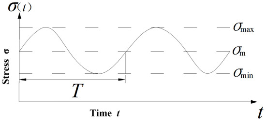
Figure 1.
The sinusoidal loading waveform diagram.
The cyclic load shown in Equation (1) can be equivalently decomposed into two parts: a constant load and a periodic dynamic load with an average value of 0. The cyclic load equivalent decomposition diagram is shown in Figure 2.
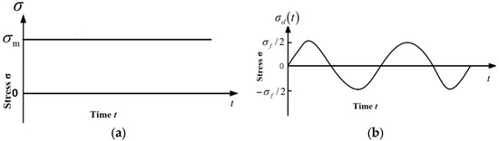
Figure 2.
The cyclic load equivalent decomposition diagram: (a) the constant load; (b) the periodic dynamic load with an average value of 0.
Although the model is developed and validated under sinusoidal loading, the decomposition of cyclic loading into static and dynamic components is general and can be extended to irregular loading patterns through cycle counting methods (e.g., rainflow counting) or harmonic decomposition via Fourier analysis. This makes the model applicable to real-world loading scenarios such as traffic vibrations, wave loads, or seismic disturbances, provided the equivalent mean stress and amplitude are appropriately defined.
2.2. The Strain Characteristics of Soft Rock Under Cyclic Loading
Under cyclic loading, the elastic deformation component of soft rock will recover during the unloading process, while the irreversible deformation (i.e., plastic deformation or residual deformation) will remain. The magnitude, growth trend, and total accumulated amount of irreversible strain serve as a more intrinsic reflection of the rock’s fatigue mechanical properties, directly related to the damage process.
Regarding the study of deformation behavior in soft rock under cyclic loading, numerous scholars have conducted extensive cyclic loading tests on various rock types [29,30,31,32,33]. Research indicates that the deformation characteristics of soft rock under cyclic loading follow distinct patterns. For both soft and hard rocks, when the upper limit of cyclic loading stress exceeds the critical strength of the rock, the irreversible deformation throughout the fatigue process can be divided into three stages (see curve II in Figure 3): initial, constant-rate, and accelerated stages. In the initial stage, deformation develops at a relatively slow rate. After a certain number of cycles, the deformation stabilizes and progresses at a constant rate. As failure approaches, the deformation accelerates significantly. Conversely, when , the strain process only comprises the initial and constant-rate stages (see curve I in Figure 3).

Figure 3.
The strain curves of rock under cyclic loading.
2.3. The Composition of Strain in Soft Rock Under Cyclic Loading
During the loading-unloading process under cyclic loading , the relationship between the applied load and the induced strain can be represented by the curve shown in Figure 4. When cyclic loading is applied for cycles, the total strain comprises two components: static strain component under static load , and dynamic strain component under dynamic load . Neglecting the influence of damage on the continuity of the strain function during loading-unloading (i.e., assuming the strain curve is a continuous function of cyclic loading time or cycle count ), the following relationship can be derived:
where is the total strain of the soft rock at time , is the dynamic strain of the soft rock at time , and is the static strain of the soft rock at time under static stress .

Figure 4.
The relationship between the applied cyclic loading and the induced strain.
2.4. The Fatigue Yield Criterion of Soft Rock
Under uniaxial cyclic loading, when , the soft rock does not undergo fatigue failure; when , the soft rock can undergo fatigue failure. Under complex stress conditions, the influence of the hydrostatic stress tensor on creep is relatively minor. Neglecting the effect of the hydrostatic stress tensor on plastic fatigue deformation and assuming that plastic fatigue deformation depends exclusively on the second deviatoric stress invariant , the fatigue yield function for soft rock under cyclic loading can be expressed as:
where is the second deviatoric stress invariant, is the maximum load value in the loading direction of the cyclic loading. When , . When , , the fatigue failure may occur in the rock. When , , the fatigue failure will not occur.
The fatigue yield criterion offers several advantages over conventional static yield criteria: (1) It explicitly incorporates the maximum cyclic stress , enabling direct modeling of fatigue-induced strength degradation; (2) It requires only one parameter (), which is readily obtainable from standard triaxial tests; (3) It naturally aligns with the three-stage deformation behavior of soft rocks under cyclic loading; (4) It avoids the need for complex damage evolution laws, making it both practical and physically interpretable. While traditional criteria such as Mohr–Coulomb or Drucker–Prager are well-suited for monotonic loading, they lack the cycle-dependent features necessary for fatigue life prediction.
The yield function in Equation (3) assumes that plastic fatigue deformation depends solely on the second deviatoric stress invariant , neglecting the influence of hydrostatic stress. This assumption is reasonable for the stress conditions considered in this study, where deformation is primarily shear-driven. However, under very high hydrostatic pressures (e.g., in deep geological environments), the mean stress may significantly affect rock behavior, leading to increased ductility and pressure-dependent yielding. In such cases, a pressure-dependent yield criterion (e.g., Drucker-Prager or modified Mohr-Coulomb) may be more appropriate. Future extensions of this model could incorporate such effects to enhance its applicability to deep rock engineering.
3. The Modified One-Dimensional Nonlinear Bingham Model Under Cyclic Loading
3.1. The One-Dimensional Unsteady Parameter Bingham Model
The traditional Bingham model is composed of a constant-viscosity dashpot and an ideal plastic slider connected in parallel, which are then connected in series with a constant elastic component. However, the conventional Bingham model fails to reflect the nonlinear deformation behavior of soft rocks. To enable it to comprehensively describe the deformation behavior of soft rocks under cyclic loading, the established non-stationary elastic component and non-constant viscosity dashpot are used to replace the constant elastic component and constant-viscosity dashpot in the traditional Bingham model, resulting in the nonlinear Bingham model for soft rocks under cyclic loading (as shown in Figure 5).
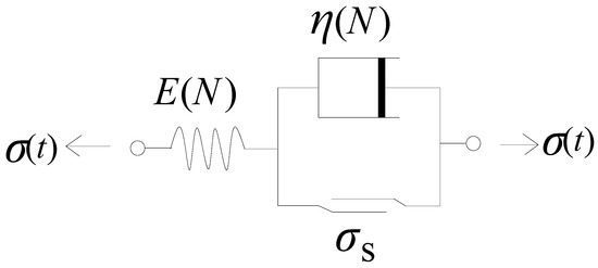
Figure 5.
The one-dimensional nonlinear Bingham model.
3.1.1. The Construction of a Dashpot Component with Non-Constant Parameters
Traditional calculus is confined to integer-order integration and differentiation, whereas fractional calculus constitutes a branch of calculus encompassing multiple formulations. Among these, the Riemann-Liouville fractional calculus is the most widely adopted. Traditional rheological models are composed of combinations of elastic bodies, plastic bodies, and ideal viscous bodies. Among these, the elastic body represents solid materials, and its mechanical model is symbolized by a spring, with the constitutive equation (or state equation) given as . The viscous body represents an ideal fluid material, and its mechanical model is depicted by a dashpot with a piston, with the constitutive equation given as . Meanwhile, the constitutive equations for the elastic body and the viscous body can be written as and , respectively. By employing the method of fractional calculus, a fractional-order dashpot representing viscoelastic materials can be constructed, with its constitutive equation given as
where is the fractional-order viscosity coefficient of the fluid, is the order of fractional-order differentiation, which is a material parameter reflecting the acceleration strain rate of the rock. Both of these material parameters can be obtained through experiments.
Schiessel et al. [34] considered the time accumulation effect of Kelvin viscous components, defined fractional elements through fractional derivatives, and constructed a fractional rheological constitutive equation. They derived that the compliance of the fractional element is proportional to , where is a constant, , and is the rheological time. Based on this, under cyclic loading , the coefficient of the viscous fatigue element in the nonlinear viscoplastic fatigue model (as shown in Figure 6) can be assumed to be proportional to , . Therefore, the dashpot component coefficient in the Bingham model is expressed as:
where is the rock strain rate parameter, , which can be determined through experiments. It mainly reflects the strain rate during the accelerated strain stage. n characterizes the transition from distributed microcracking to localized shear band formation. Higher n values indicate faster microstructural degradation rates. When , the model degenerates into the traditional Bingham model. is a non-zero constant, which is the initial viscous coefficient (unit: Pa·s) of the nonlinear Bingham model and mainly reflects the viscous characteristics of soft rock. represents the initial viscous resistance stemming from intergranular friction and cementation bonds. As cyclic loading progresses, these bonds degrade, reducing and enabling faster plastic deformation. The power-law decay of the viscous coefficient captures the accelerated viscous flow due to progressive breakdown of internal friction and cementation bonds under cyclic loading.
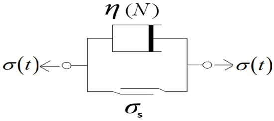
Figure 6.
The nonlinear viscoplastic body.
The state equation for the non-constant dashpot component is expressed as:
When , substituting Equation (5) into Equation (6), and then integrating Equation (6) to obtain
3.1.2. The Construction of an Elastic Component with Non-Constant Parameters
Under cyclic loading, the strength of soft rock gradually decreases as the loading time increases. The reduction in the strength of soft rock will inevitably lead to the weakening of its strength parameters over time. This phenomenon also reveals the creep damage mechanism of soft rock. Studies have shown that under cyclic loading, the elastic modulus decreases exponentially with the number of cycles or loading time. By fitting the attenuation curve and based on the concept of rheology mechanics, it can be assumed that the coefficient of the elastic component (as shown in Figure 7) decreases exponentially with the number of load applications . The attenuation law is expressed as:
where is the initial value of the elastic component coefficient in the Bingham model, mainly reflecting the elastic properties of soft rock; is the dimensionless parameter for controlling the change in the elastic coefficient. It characterizes the relationship between the elastic coefficient and the strain rate in the first two stages of soft rock deformation, can be determined through experiments, and its value is greater than zero. λ directly quantifies the rate of elastic modulus degradation in soft rocks under cyclic loading. As microcracks propagate and grain contacts weaken during initial deformation stages (Stages I–II), λ increases due to reduced energy dissipation capacity, eventually stabilizing when microstructure reaches a critical damage threshold. The exponential decay of the elastic modulus E with cycle number N reflects the cumulative microstructural damage in soft rock, such as crack propagation and bond degradation, which reduces the material’s ability to store elastic energy.
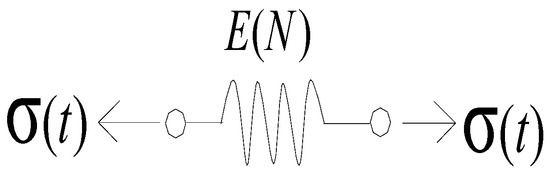
Figure 7.
The nonlinear elastic element body.
3.2. The Constitutive Equation of the One-Dimensional Nonlinear Bingham Model
3.2.1. The Static Strain Under Static Load
According to the one-dimensional nonlinear Biham model shown in Figure 5, the stress on each component of the series-connected components is equal, and the strain is equal to the sum of the strains of each component, which leads to
where and represent the stress on the elastic element and the viscous element, respectively, and represent the corresponding strains, respectively. Equations (9) and (10) can be further rewritten as
According to Equations (7), (8), (11) and (12), the constitutive equation of the one-dimensional nonlinear Bingham model under static load can be obtained as
when , . At this point, the soft rock strain is the instantaneous elastic strain under the static load .
3.2.2. The Dynamic Strain Under Dynamic Load
According to the theory of viscoelastic mechanics, it can be considered that the deformation process of soft rock under cyclic loading is a process of continuous energy storage and dissipation. The strain and stress changes in an ideal elastic solid material are in phase. For an ideal viscous material, the time lag between strain and stress is . For general materials, it lies between the two extremes. The response strain does not have the same phase as the cyclic loading . There is a phase difference between stress and strain, also known as the phase angle of strain lagging behind stress or the energy dissipation angle, which is expressed as , and represent the elastic energy storage quantity and the elastic energy consumption quantity, respectively. quantifies the material’s reversible energy storage capacity during cyclic loading. It is directly related to the elastic deformation mechanism, representing the portion of strain energy that can be recovered after unloading. Physically, it reflects the material’s ability to temporarily store mechanical energy via atomic/molecular bond stretching or microstructure reorientation. characterizes the irreversible energy dissipation capacity due to viscous or plastic deformation. It accounts for energy loss via internal friction, micro-crack propagation, or inelastic deformation. Unlike , is frequency-dependent and increases with loading rate in many materials. and are not directly measured but are model-derived parameters expressed in terms of the time and cycle dependent material properties (e.g., elastic modulus E(N) and viscous parameter η(N). Specifically, and are functions of the cyclic loading frequency and the degrading material properties. Their expressions can be derived from the constitutive relations of the nonlinear Bingham model, incorporating the decay functions for elasticity and viscosity.
According to the visco-elastic-plastic principle [35], the dynamic strain under cyclic loading is expressed as
where
According to Equation (15), it can be obtained:
3.2.3. The Constitutive Equation of the One-Dimensional Nonlinear Bingham Model
By adding the static strain and the dynamic strain , the total strain of the one-dimensional nonlinear Bingham model under cyclic loading can be obtained.
By combining Equations (13) and (18), we can obtain
By combining Equations (14) and (19), we can obtain
4. The Modified 3-D Nonlinear Bingham Model Under Cyclic Loading
The one-dimensional nonlinear Bingham model developed in Section 3 effectively captures the fatigue deformation characteristics of soft rock under uniaxial cyclic loading. However, rock masses in engineering applications are typically subjected to complex three-dimensional stress states. Extending the 1D model to 3D requires generalizing the nonlinear elastic and viscoplastic fatigue components within a tensorial framework, while ensuring the model remains consistent with the principles of continuum mechanics and the specific failure mechanisms of soft rock under cyclic loading. This section details this generalization process, which primarily involves: (1) Replacing the scalar stress and strain in the 1D model with their tensorial counterparts (stress tensor and strain tensor); (2) Decomposing the stress and strain tensors into spherical and deviatoric components, assuming the volumetric strain of the viscoplastic component is negligible and that plastic fatigue deformation is driven primarily by deviatoric stress; (3) Generalizing the decay laws for the elastic shear modulus and the viscous parameter, originally functions of cycle number N, into the 3D formulation; (4) Incorporating a fatigue yield criterion to determine the onset and evolution of viscoplastic flow in the multiaxial stress space; (5) Adopting an associated flow rule to define the direction of the viscoplastic strain rate tensor.
4.1. The 3-D Unsteady Parameter Bingham Model
The three-dimensional nonlinear Bingham model is composed of a three-dimensional unsteady elastic fatigue component and a nonlinear viscoplastic fatigue component (as shown in Figure 8). In the model, is the elastic shear fatigue coefficient related to the number of cycles, is the expression of the soft rock fatigue yield function, and is the equivalent deviatoric stress tensor.

Figure 8.
The three-dimensional nonlinear Bingham model.
4.1.1. The Three-Dimensional Nonlinear Elastic Fatigue Component
From the construction of one-dimensional elastic fatigue component, it can be known that the elastic coefficient E decreases exponentially with the number of cycles or loading time under cyclic loading. For three-dimensional elastic fatigue elements, the shear coefficient is related to the elastic coefficient E as , where is Poisson’s ratio and is a constant. Thus, it can be concluded that the shear coefficient is proportional to the elastic coefficient E. Therefore, it can be assumed that the coefficient of the three-dimensional elastic component (as shown in Figure 9) also continuously decays exponentially with the number of load applications, and the decay rule is
where is the initial value of the shear coefficient of the three-dimensional Bingham model.
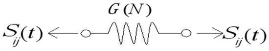
Figure 9.
The three-dimensional nonlinear elastic component.
The state equation is
where is the first invariant of the stress tensor; is the equivalent deviatoric stress tensor; is the spherical stress (i.e., the average stress), the elastic fatigue cumulative strain tensor, is the first invariant of the elastic fatigue strain tensor, K is the fatigue volume modulus.
Substituting Equation (22) into Equation (23), the cumulative strain of the three-dimensional elastic fatigue element is obtained as
where is the spherical strain tensor of the elastic component.
4.1.2. The Three-Dimensional Nonlinear Viscoplastic Fatigue Component
The three-dimensional nonlinear viscoplastic fatigue component is shown in Figure 10. In the model, the unsteady shear viscoplastic fatigue coefficient is the same as Equation (5).
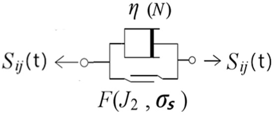
Figure 10.
The three-dimensional nonlinear viscoplastic component.
The three-dimensional constitutive relationship of the viscoplastic component [36,37] is:
where is the strain of the viscoplastic component, is the fatigue yield function of soft rock, as shown in Equation (3), is the initial value of the fatigue yield function of soft rock, is the fatigue plastic potential function, is in the form of an exponential function, and the power exponent is usually set to 1.
Here, the associated flow rule is adopted, where the plastic potential function is set to be equal to the yield function F. This choice is consistent with the J2 plasticity theory and is widely used in geomechanical models for rocks under deviatoric dominated fatigue loading [3,36]. It implies that the direction of the plastic strain increment is normal to the yield surface, which is a reasonable assumption for shear fatigue failure in soft rocks. Although non-associated flow rules may be more appropriate for pressure sensitive materials, the associated rule is retained here for simplicity and numerical stability. By adopting the flow rule associated with the yield criterion, when , the soft rock does not undergo fatigue deformation. When , set the initial yield function . Substituting Equation (5) into Equation (25) yields
under the condition of equal triaxial confining pressure, that is, , .
4.2. The Constitutive Equation of the Three-Dimensional Nonlinear Bingham Model
4.2.1. The Static Strain Under Static Load
Ignoring the volumetric strains of elastic fatigue components and viscoplastic fatigue components. Under the static load , by superimposing the cumulative strain of the elastic fatigue component and the cumulative strain of the viscoplastic fatigue component, the constitutive equation for the total static strain under the static load can be obtained as
4.2.2. The Dynamic Strain Under Dynamic Load
Under cyclic loading, assuming that the deformation behavior of the soft rock starts from a small deformation state, then in the three-dimensional case, the dynamic stress can be expressed as
where is the imaginary unit.
Under the dynamic load , the response dynamic strain is
where is the dynamic strain in the loading direction of the dynamic load at time t, its expression and its plural form are, respectively:
where is the complex amplitude of the response in the dynamic load direction, is the amplitude of the response in the dynamic load direction, and the expression is
where and are the storage flexibility quantity and the dissipation flexibility quantity of the modified three-dimensional nonlinear Bingham model, respectively. They are expressed as:
According to Equations (31)–(34), the dynamic response constitutive equation of the three-dimensional Bingham model that reflects the dynamic strain characteristics of soft rock in the direction of dynamic loading is
The calculation of the dynamic strains and in the direction of confining pressure under dynamic loads can be obtained through Equation (30).
4.2.3. The Constitutive Equation of the Three-Dimensional Nonlinear Bingham Model
Based on the composition of the strain of soft rock under cyclic loading, by superimposing the static strain and dynamic strain of soft rock under three-dimensional loading conditions, the total strain of the three-dimensional nonlinear Bingham model under cyclic loading can be obtained. By superimposing Equations (27) and (35), as well as (28) and (36), the constitutive equation of the three-dimensional Bingham model that reflects the dynamic strain characteristics of soft rock in the direction of dynamic loading can be expressed as
The calculations of strains and in the direction of confining pressure can be obtained by superimposing Equation (39) onto Equations (27) and (28), respectively. When the confining pressure is constant, that is, , according to Equations (37) and (38), the constitutive equation of soft rock under the dynamic triaxial equal confining pressure condition is
5. The Adaptability Validation and Parameter Identification for the Modified 3D Nonlinear Bingham Model
In this paper, the Powell Optimization (OP) algorithm is employed to perform curve fitting and parameter determination for the model. Based on the relevant experimental data, the constitutive Equations (39) and (40) under low dynamic stress conditions () and high dynamic stress conditions () are, respectively, fitted to verify the adaptability of the model, followed by identification of the model parameters.
5.1. Adaptive Verification of the Modified 3D Nonlinear Bingham Model Under the Condition
Ding et al. [38] conducted a cyclic dynamic triaxial test on water-rich sandy mudstone under sinusoidal cyclic loading by using the MTS rock dynamic system, with a confining pressure of 200 kPa applied. The research found that under the conditions of confining pressure = 200 kPa, static deviatoric stress = 180 kPa, and loading frequency of 3 Hz, the critical dynamic stress amplitude = 240 kPa. Therefore, the critical strength of the water-rich sandy mudstone is = 300 kPa, the static stress in the direction of the dynamic load is = 380 kPa, and the maximum stress in the direction of the dynamic load is = 500 kPa. The relevant test parameters of the rich-water sandy mudstone is shown in Table 1.

Table 1.
The dynamic test parameters of the rich-water sandy mudstone [38].
When the amplitude of the cyclic loading dynamic stress is , . At this point, the mudstone only undergoes the first two stages of deformation: deceleration and constant speed. The constitutive Equation (39) proposed for soft rocks under low dynamic stress conditions was employed to fit the experimental data of cumulative plastic strain versus cyclic loading number N for water-rich sandy mudstone under low dynamic stress. The fitted curves are shown in Figure 11, and the fitting results are presented in Table 2.
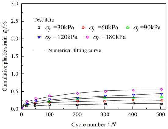
Figure 11.
The numerical fitting curve of cumulative plastic strain under different low dynamic stress amplitudes.
Table 2.
The fitting results for water-rich sandy mudstone under .
The fitted curves and results demonstrate that under low dynamic stress conditions, the constitutive equation of the 3D nonlinear Bingham model developed in this study exhibits high agreement with experimental data, with all fitting correlation coefficients exceeding 0.978. Furthermore, the model effectively characterizes the deformation behavior of soft rocks during the first two stages (deceleration and constant speed phases) under low dynamic stress. This validates the correctness and rationality of the developed 3D nonlinear Bingham fatigue constitutive model under low dynamic stress conditions.
5.2. Adaptive Verification of the Modified 3D Nonlinear Bingham Model Under the Condition
In the cyclic dynamic triaxial test of water-rich sandy mudstone, when the amplitude of the cyclic loading dynamic stress is , . At this point, mudstone can undergo three complete stages of deformation: deceleration, constant speed, and acceleration. The constitutive Equation (40) proposed for soft rocks under high dynamic stress conditions was employed to fit the experimental data of cumulative plastic strain versus cyclic loading number N for water-rich sandy mudstone under high dynamic stress. The fitted curves are shown in Figure 12, and the fitting results are presented in Table 3.

Figure 12.
The numerical fitting curve of cumulative plastic strain under high dynamic stress amplitude for the water-rich sandy mudstone.
Table 3.
The fitting results of different soft rock test data under .
Zhang et al. [39] conducted triaxial fatigue deformation characteristic tests on red sandstone, applying sinusoidal cyclic loading with a frequency of 0.2 Hz. The upper and lower stress limits of the cyclic loading were 51.8 MPa and 99.1 MPa, respectively, resulting in a load amplitude of = 47.3 MPa. According to the cyclic loading equivalence principle, the applied cyclic loading can be decomposed into a constant load component of = 75.45 MPa and a cyclic dynamic load component of = 23.65 MPa with a mean value of zero. The critical strength of red sandstone under a confining pressure 15 MPa is = 98.22 MPa. Therefore, the triaxial fatigue deformation test of red sandstone is a fatigue test conducted under high dynamic stress, at this time . The constitutive Equation (40) proposed for soft rocks under high dynamic stress conditions was employed to fit the experimental data of cumulative plastic strain versus cyclic loading number N for red sandstone under high dynamic stress. The fitted curves are shown in Figure 13, and the fitting results are presented in Table 3.
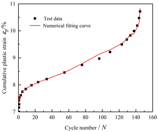
Figure 13.
The numerical fitting curve of cumulative plastic strain under high dynamic stress amplitude for the red sandstone.
The fitting curves and results for water-rich sandy mudstone and red sandstone demonstrate that under high dynamic stress conditions, the proposed three-dimensional nonlinear Bingham model constitutive equation aligns well with experimental data, with correlation coefficients of the fits exceeding 0.989. Furthermore, this model effectively captures the complete deformation characteristics of soft rocks under high dynamic stress, including the deceleration, constant velocity, and acceleration stages. Consequently, it validates the accuracy and rationality of the established three-dimensional nonlinear Bingham fatigue constitutive model for high dynamic stress conditions.
5.3. Parameter Identification of the Three-Dimensional Nonlinear Bingham Model
5.3.1. Parameter Identification When
In order to better illustrate the variation trend of parameter λ with the dynamic stress amplitude, we have added several dynamic stress amplitudes of = 105, 135 and 150 kPa, and the corresponding parameters λ are 0.301, 0.330 and 0.334, respectively. Under low dynamic stress conditions, the parameter associated with the elastic shear fatigue parameter increases with the dynamic load amplitude and eventually stabilizes, as illustrated in Figure 14. The variation in parameter reflects the evolution pattern of the elastic shear fatigue parameter and also characterizes the strain rate of soft rocks during the initial two deformation stages. By comparing the curve of versus dynamic load amplitude with the curve of soft rock strain versus cyclic loading number N for the first two stages, a strong similarity is observed. This indicates that as external dynamic loads increase, the crystalline structure of soft rocks undergoes changes accompanied by internal energy dissipation, leading to a reduction in their capacity to resist external stresses. Subsequently, the crystalline structure stabilizes, resulting in constant internal energy changes and a steady resistance capacity. This transition macroscopically corresponds to the initial two deformation stages of soft rocks under low dynamic stress conditions.
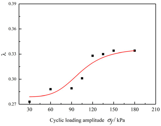
Figure 14.
The relationships between and , when .
5.3.2. Parameter Identification When
- Sensitivity analysis on parameter n
Under high dynamic stress conditions (i.e., ), the primary focus is on identifying the strain rate parameter n that characterizes the accelerated deformation stage of soft rocks. According to fractional calculus theory, n is constrained within 0 < n < 1. When n = 1, the viscoplastic fatigue component reduces to the conventional viscoplastic component in the classical Bingham model, which fails to describe the accelerated strain stage of soft rocks. To investigate the effect of parameter n on soft rock strain, values of n = 0.100, 0.200, 0.400, 0.600, 0.800, and 0.900 were selected while keeping other parameters constant. The relationship between cumulative plastic strain and cyclic loading number N under different n values was analyzed, with the influence curves illustrated in Figure 15. As shown in the figure, during the third deformation stage (accelerated deformation) of soft rocks, the cumulative strain in the fatigue constitutive model increases with higher n. This validates that parameter n reasonably reflects the strain characteristics during the accelerated deformation phase of soft rocks.
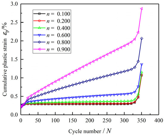
Figure 15.
The influence of different parameter on the plastic cumulative strain .
It is noteworthy that the strain rate parameter n also influences the accumulated strain rate during the second stage (i.e., the constant velocity stage). A larger n leads to a higher accumulated strain rate. This indicates that, under the same stress level, a greater n results in a faster strain rate, directly causing an increase in the accumulated strain rate during the constant velocity stage. The increase in n may reflect changes in the deformation mechanism. When dislocation slip dominates (low n), the strain hardening effect is weaker; however, when grain boundary sliding or diffusion-controlled mechanisms prevail (high n), the material becomes more prone to strain accumulation, leading to a rise in the accumulated strain rate. This phenomenon highlights the critical role of n in regulating the deformation behavior of materials, providing a theoretical basis for optimizing their deformation resistance.
- 2.
- Sensitivity analysis on parameter λ
The parameter λ, governing the exponential decay of the elastic shear modulus (Equation (22)), significantly influences the cumulative plastic strain development, particularly during the acceleration stages. Figure 16 illustrates the relationship between the cumulative plastic strain and the number of cycles N for different values of λ (λ = 0.80, 0.81, 0.82, 0.83, 0.84 and 0.85), while keeping other parameters constant. A higher λ value indicates a faster rate of elastic modulus degradation. Consequently, as λ increases, the strain accumulated during the acceleration stage becomes more pronounced. This occurs because a rapidly degrading elastic modulus reduces the material’s capacity to store elastic energy reversibly, leading to greater energy dissipation and accelerated accumulation of irreversible plastic deformation from earlier cycles. This sensitivity analysis confirms that λ effectively captures the damage evolution and stiffness reduction in soft rock of cyclic loading. The strain rate exhibits a three-phase behavior: initial rapid growth, stabilized development, and accelerated phase, which is consistent with the theoretical framework of the model.
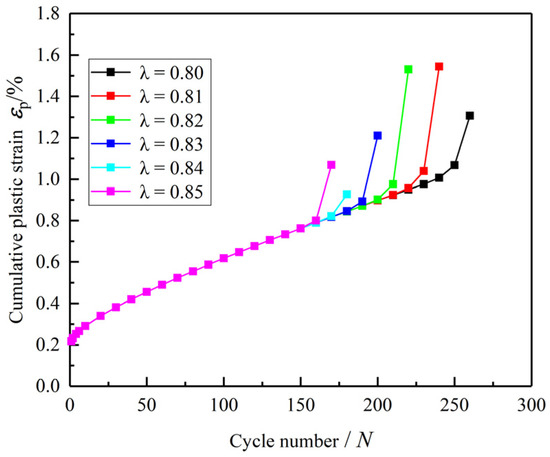
Figure 16.
The influence of different parameter λ on the plastic cumulative strain .
- 3.
- Sensitivity analysis on parameter
The initial viscous coefficient , representing the initial intergranular friction and cementation bond strength (Equation (5)), primarily governs the strain rate during the constant velocity stage (Stage II). Figure 17 presents the effect of varying ( = 5 MPa, 10 MPa, 15 MPa, 20 MPa and 25 MPa) on the cumulative plastic strain versus cycle number N curve, with other parameters held constant. A larger signifies higher initial viscous resistance, which directly results in a lower constant strain rate during the secondary stage. Conversely, a smaller leads to a higher strain rate in Stage II, indicating less resistance to viscous flow. This parameter crucially influences the duration of the constant velocity stage; higher values typically prolong this stage before the potential onset of accelerated creep (Stage III), provided the stress conditions allow for it. Thus, is a key parameter for calibrating the rate of deformation before significant damage accumulation triggers the tertiary stage.
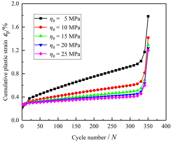
Figure 17.
The influence of different parameter on the plastic cumulative strain .
5.4. Discussion on Model Applicability to Other Soft Rocks
Although the model has been validated only against water-rich sandy mudstone and red sandstone, its theoretical framework is general and applicable to other types of soft rocks (e.g., salt rock, coal measure soft rock, shale) under cyclic loading. The model captures key deformation mechanisms such as nonlinear elasticity decay, viscosity evolution, and accelerated creep, which are common in many soft rocks. However, the specific values of parameters such as G0, η0, n, and α may vary across different rock types and should be determined through experimental calibration. Future work should include validation against a broader range of soft rocks to further verify the model’s generalizability.
6. Conclusions
This paper develops a modified Bingham fatigue model to describe the strain characteristics of soft rock under cyclic loading. Based on the traditional Bingham model in the theory of rheology, the constant viscosity component in the model is replaced by a variable coefficient viscosity component related to the number of cycles, and the elastic component is replaced by a non-fixed elastic component that decays with the increase in the number of cycle loads. The cyclic loading is decomposed into fixed load and alternating load. A one-dimensional nonlinear viscoelastic-plastic Bingham fatigue constitutive model reflecting the various strain laws of soft rock under cyclic loading is established. A rock fatigue yield criterion is proposed, and the flow criterion related to this fatigue yield criterion is adopted to extend the one-dimensional fatigue constitutive model to a three-dimensional fatigue constitutive model under complex stress conditions. The model is verified for its adaptability, and the parameters of the model are identified. The validation against experimental data for water-rich sandy mudstone and red sandstone shows that the model achieves correlation coefficients above 0.978 and 0.989 under low and high dynamic stress conditions, respectively, with RMSE values as low as 0.005–0.028. Key parameters such as the strain rate parameter n and the elastic decay parameter λ were identified and shown to physically reflect the deformation mechanisms. Compared with the existing fatigue test results of soft rock, the improved Bingham fatigue constitutive model can better describe the three complete fatigue deformation processes of soft rock under cyclic loading, and the model has fewer components and a simple combination form, providing a reference for the study of rock fatigue deformation characteristics under dynamic loads.
Author Contributions
Investigation, Y.L. (Yonghui Li) and Y.L. (Yi Liang); Data curation, F.Z.; Writing—original draft, Y.L. (Yonghui Li); Writing—review and editing, Y.L. (Yonghui Li); Visualization, A.S.; Supervision, Y.L. (Yi Liang). All authors have read and agreed to the published version of the manuscript.
Funding
This research was funded by the Guizhou Provincial Basic Research Program (Natural Science) General Project (Qiankehe Foundation MS[2025]199), the Guizhou Institute of Technology Academic New Talent Cultivation and Innovative Exploration Project (2024XSXM013), the Guizhou Institute of Technology High-Caliber Talent Recruitment Program (2025GCC028), and the Guizhou Province science and technology plan project (Qiankehe Platform KXJZ[2024]020).
Data Availability Statement
The original contributions presented in this study are included in the article. Further inquiries can be directed to the corresponding author.
Conflicts of Interest
The authors declare no conflicts of interest.
References
- Yang, D.; Qiu, X. A Constitutive Model for Rock Joints under Cyclic Loading. Adv. Mater. Res. 2011, 243–249, 2211–2215. [Google Scholar] [CrossRef]
- Zang, M.; Kong, L.; Zhang, R.; Wang, W. Simplified Calculation Method for Cumulative Deformations of Marine Structured Clay under Cyclic Loading. Arab. J. Geosci. 2021, 14, 945. [Google Scholar] [CrossRef]
- Zhou, Y.; Sheng, Q.; Li, N.; Fu, X.; Zhang, Z. A Dynamic Constitutive Model for Rock Materials Subjected to Medium- and Low-Strain-Rate Dynamic Cyclic Loading. J. Eng. Mech. 2022, 148, 11. [Google Scholar] [CrossRef]
- Yu, D.; Liu, E.; Sun, P.; Xing, H.; Zheng, Q. Dynamic Mechanical Properties and Constitutive Model for Jointed Mudstone Samples Subjected to Cyclic Loading. Eur. J. Environ. Civ. Eng. 2022, 26, 7240–7266. [Google Scholar] [CrossRef]
- Wichtmann, T.; Triantafyllidis, T. An Experimental Database for the Development, Calibration and Verification of Constitutive Models for Sand with Focus to Cyclic Loading: Part II—Tests with Strain Cycles and Combined Loading. Acta Geotech. 2016, 11, 763–774. [Google Scholar] [CrossRef]
- Wichtmann, T.; Triantafyllidis, T. An Experimental Database for the Development, Calibration and Verification of Constitutive Models for Sand with Focus to Cyclic Loading: Part I—Tests with Monotonic Loading and Stress Cycles. Acta Geotech. 2016, 11, 739–761. [Google Scholar] [CrossRef]
- Yu, Y.; Yang, Y.; Liu, J.; Wang, P.; Zhang, S.; Wang, Z.; Zhao, S. Experimental and Constitutive Model Study on the Mechanical Properties of a Structural Plane of a Rock Mass under Dynamic Disturbance. Sci. Rep. 2022, 12, 21238. [Google Scholar] [CrossRef]
- Liu, X.S.; Ning, J.G.; Tan, Y.L.; Gu, Q.H. Damage Constitutive Model Based on Energy Dissipation for Intact Rock Subjected to Cyclic Loading. Int. J. Rock Mech. Min. Sci. 2016, 85, 27–32. [Google Scholar] [CrossRef]
- Meng, X.; Zhang, H.; Yuan, C.; Li, Y.; Liu, X.; Chen, S.; Shen, Y. Damage Constitutive Prediction Model for Rock under Freeze–Thaw Cycles Based on Mesoscopic Damage Definition. Eng. Fract. Mech. 2023, 293, 109685. [Google Scholar] [CrossRef]
- He, W.; Wu, Y.F.; Liew, K.M. A Fracture Energy Based Constitutive Model for the Analysis of Reinforced Concrete Structures under Cyclic Loading. Comput. Methods Appl. Mech. Eng. 2008, 197, 4745–4762. [Google Scholar] [CrossRef]
- Wu, T.; Nie, L.; Cai, Z.; Wu, Y.; Shi, Q.; Lin, J.; Wang, K.; Xu, N. Development of a Model for Initial Compaction Stage in Rock Based on Energy Dissipation. Adv. Mater. Sci. Eng. 2022, 2022, 7186594. [Google Scholar] [CrossRef]
- Shutov, A.; Larichkin, A.; Shutov, V. Modelling of Large Strain Creep with Static and Dynamic Recovery under Cyclic Loading Conditions. PAMM 2017, 17, 463–464. [Google Scholar] [CrossRef]
- Zhang, L.; Wang, X. Study on Nonlinear Damage Creep Model for Rocks under Cyclic Loading and Unloading. Adv. Mater. Sci. Eng. 2021, 2021, 5512972. [Google Scholar] [CrossRef]
- Wang, X.; Song, L.; Xia, C.; Han, G.; Zhu, Z. Nonlinear Elasto-Visco-Plastic Creep Behavior and New Creep Damage Model of Dolomitic Limestone Subjected to Cyclic Incremental Loading and Unloading. Sustainability 2021, 13, 12376. [Google Scholar] [CrossRef]
- Zienkiewicz, O.C.; Cormeau, I.C. Visco-plasticity—Plasticity and Creep in Elastic Solids—A Unified Numerical Solution Approach. Int. J. Numer. Methods Eng. 1974, 8, 821–845. [Google Scholar] [CrossRef]
- Yang, S.Q.; Xu, P.; Xu, T. Nonlinear Visco-Elastic and Accelerating Creep Model for Coal under Conventional Triaxial Compression. Geomech. Geophys. Geo-Energy Geo-Resour. 2015, 1, 109–120. [Google Scholar] [CrossRef]
- Zhou, H.; Jia, Y.; Shao, J.F. A Unified Elastic-Plastic and Viscoplastic Damage Model for Quasi-Brittle Rocks. Int. J. Rock Mech. Min. Sci. 2008, 45, 1237–1251. [Google Scholar] [CrossRef]
- Hou, R.; Zhang, K.; Tao, J.; Xue, X.; Chen, Y. A Nonlinear Creep Damage Coupled Model for Rock Considering the Effect of Initial Damage. Rock Mech. Rock Eng. 2019, 52, 1275–1285. [Google Scholar] [CrossRef]
- Liu, H.Z.; Xie, H.Q.; He, J.D.; Xiao, M.L.; Zhuo, L. Nonlinear Creep Damage Constitutive Model for Soft Rocks. Mech. Time-Depend. Mater. 2017, 21, 73–96. [Google Scholar] [CrossRef]
- Ping, C.; Wen, Y.; Wang, Y.; Yuan, H.; Yuan, B. Study on Nonlinear Damage Creep Constitutive Model for High-Stress Soft Rock. Environ. Earth Sci. 2016, 75, 900. [Google Scholar] [CrossRef]
- Mo, H. Investigation of Cyclic Loading Tests and Constitutive Relation of Rock. Chin. J. Rock Mech. Eng. 1988, 7, 215–224. [Google Scholar]
- Wang, J.B.; Liu, X.R.; Huang, M.; Yang, X. Analysis of Axial Creep Properties of Salt Rock under Low Frequency Cyclic Loading Using Burgers Model. Yantu Lixue/Rock Soil Mech. 2014, 35, 933–942. [Google Scholar]
- Guo, J.Q.; Huang, Z.H. Constitutive Model for Fatigue of Rock under Cyclic Loading. Yantu Gongcheng Xuebao/Chin. J. Geotech. Eng. 2015, 37, 1698–1704. [Google Scholar] [CrossRef]
- Wang, J.; Wang, T.; Song, Z.; Zhang, Y.; Zhang, Q. Improved Maxwell Model Describing the Whole Creep Process of Salt Rock and Its Programming. Int. J. Appl. Mech. 2021, 13, 2150113. [Google Scholar] [CrossRef]
- Rezaiee-Pajand, M.; Masoodi, A.R. Hygro-thermo-elastic nonlinear analysis of functionally graded porous composite thin and moderately thick shallow panels. Mech. Adv. Mater. Struct. 2020, 29, 594–612. [Google Scholar] [CrossRef]
- Rezaiee-Pajand, M.; Rajabzadeh-Safaei, N.; Masoodi, A.R. An efficient curved beam element for thermo-mechanical nonlinear analysis of functionally graded porous beams. Structures 2020, 28, 1035–1049. [Google Scholar] [CrossRef]
- Li, X.; Wu, D.; Wu, M. Creep characteristics and fractional rheological model of granite under temperature and disturbance load coupling. Mech. Time-Depend. Mater. 2024, 28, 18. [Google Scholar] [CrossRef]
- Cai, S.M.; Chen, Y.M.; Liu, Q.X. Development and validation of fractional constitutive models for viscoelastic-plastic creep in time-dependent materials: Rapid experimental data fitting. Appl. Math. Model. 2024, 132, 645–678. [Google Scholar] [CrossRef]
- Ge, X. Study on Deformation and Strength Behaviour of the Large-Sized Triaxial Rock Samples under Cyclic Loading. Chin. J. Rock Soil Mech. 1987, 8, 11–19. [Google Scholar]
- Lin, Z.; Wu, Y. Strength and Deformability of Rock under Cyclic Loading. Chin. J. Rock Soil Mech. 1987, 8, 31–37. [Google Scholar]
- Xu, J.G.; Zhang, P.; Li, N. Deformation Properties of Rock Mass with Intermittent Cracks under Cyclic Loading. Yantu Gongcheng Xuebao/Chin. J. Geotech. Eng. 2008, 30, 802–806. [Google Scholar]
- Peckley, D.C.; Uchimura, T. Strength and Deformation of Soft Rocks under Cyclic Loading Considering Loading Period Effects. Soils Found. 2009, 49, 51–62. [Google Scholar] [CrossRef]
- Zhao, Y.; Dang, S.; Bi, J.; Wang, C.-L.; Gan, F. Influence of Complex Stress Path on Energy Characteristics of Sandstones under Triaxial Cyclic Unloading Conditions. Int. J. Geomech. 2022, 22, 04022076. [Google Scholar] [CrossRef]
- Schiessel, H.; Metzler, R.; Blumen, A.; Nonnenmacher, T.F. Generalized Viscoelastic Models: Their Fractional Equations with Solutions. J. Phys. A Gen. Phys. 1995, 28, 6567–6584. [Google Scholar] [CrossRef]
- Christensen, R.M.; Freund, L.B. Theory of Viscoelasticity. J. Appl. Mech. 1971, 38, 720. [Google Scholar] [CrossRef]
- Zienkiewicz, O.C.; Owen, D.R.J.; Cormeau, I.C. Analysis of Viscoplastic Effects in Pressure Vessels by the Finite Element Method. Nucl. Eng. Des. 1974, 28, 278–288. [Google Scholar] [CrossRef]
- Gioda, G. A Finite Element Solution of Non-Linear Creep Problems in Rocks. Int. J. Rock Mech. Min. Sci. 1981, 18, 35–46. [Google Scholar] [CrossRef]
- Ding, Z.; Peng, L.; Shi, C.; Luo, J.; Yang, W. Experimental Study on Dynamic Deformation Behaviors of Water-Rich Sandy Mudstone under Cyclic Loading. Chin. J. Geotech. Eng. 2012, 34, 534–539. [Google Scholar] [CrossRef]
- Zhang, Q.X.; Ge, X.R.; Huang, M.; Sun, H. Testing Study on Fatigue Deformation Law of Red-Sandstone under Triaxial Compression with Cyclic Loading. Yanshilixue Yu Gongcheng Xuebao/Chin. J. Rock Mech. Eng. 2006, 25, 473–478. [Google Scholar]
Disclaimer/Publisher’s Note: The statements, opinions and data contained in all publications are solely those of the individual author(s) and contributor(s) and not of MDPI and/or the editor(s). MDPI and/or the editor(s) disclaim responsibility for any injury to people or property resulting from any ideas, methods, instructions or products referred to in the content. |
© 2025 by the authors. Licensee MDPI, Basel, Switzerland. This article is an open access article distributed under the terms and conditions of the Creative Commons Attribution (CC BY) license (https://creativecommons.org/licenses/by/4.0/).