Bounds on Causal Effects Based on Expectations in Ordered-Outcome Models

Abstract

Bounding causal effects under unmeasured confounding is particularly challenging when the outcome variable is ordinal. When the goal is to assess whether an intervention leads to a better outcome, ordinal causal effects offer a more appropriate analytical framework. In contrast, the average causal effect (ACE), defined as the difference in expected outcomes, is more suitable for capturing population-level effects. In this paper, we derive sharp bounds for causal effects with ternary outcomes using an expectation-based framework, under both general conditions and monotonicity assumptions. We conduct numerical simulations to evaluate the width of the bounds under various scenarios. Finally, we demonstrate our method’s practical utility by applying it to the CDC Diabetes Health Indicators Dataset to assess the causal effect of health behaviors on diabetes risk.

1. Introduction

Currently, research on causal inference remains primarily focused on scenarios involving binary variables, such as evaluating the causal effect of an exposure on an outcome when both are binary [1,2]. However, in real-world applications, variables are often not restricted to binary values, and may instead take multiple or continuous forms. In these more complex settings, causal inference faces greater challenges, particularly in the presence of unmeasured confounders, which makes the accurate estimation of causal effects a critical concern. Consequently, exploring causal inference methods that are suitable for multivalued variables and establishing reasonable bounds for causal effects under unmeasured confounding are of substantial theoretical and practical importance.

Causal inference in the presence of incomplete compliance and unmeasured confounders typically cannot precisely identify causal effects, but nonparametric bounds can be used to narrow the range of plausible values. Balke and Pearl [3] introduced a method for calculating counterfactual probabilities and derived causal effect bounds based on observable conditional distributions. Building on this, Balke and Pearl [1] further investigated treatment effect estimation under incomplete compliance and proposed the tightest nonparametric bounds. Their work laid the foundation for using linear programming as a tool to derive causal bounds in the presence of unmeasured confounding. This approach has since been extended to a variety of complex settings, including missing data [4], Mendelian randomization [5], and mediation analysis [6].

While these methods were initially developed for binary treatment and outcome variables, the general principle of bounding causal effects without strong parametric assumptions has proven adaptable to more complex settings. In particular, recent research has extended these ideas to causal inference with ordinal outcomes, where identification challenges remain and full identification is often infeasible.

The potential outcomes framework, first introduced by Neyman [7] and later formalized by Rubin [8], provides a foundation for causal inference by defining causal effects as comparisons between potential outcomes under different treatment assignments. Traditionally, the ACE has been the primary causal estimand within this framework. However, as the field has advanced, increasing attention has been devoted to settings where treatments or outcomes are ordinal or continuous, leading to new definitions and identification strategies for causal parameters.

Despite this progress, much of the existing literature has continued to focus on the ACE and its variants, with relatively limited attention paid to ordinal outcomes. Rosenbaum [9] examined causal inference for ordinal outcomes under a monotonicity assumption, where treatment effects are assumed to be non-negative for all individuals. Agresti and Kateri [10] and Cheng [11] considered the assumption of independence between potential outcomes, in both explicit and implicit forms.

Huang et al. [12] derived numerical bounds on the probability that treatment is beneficial and strictly beneficial, while Lu et al. [13] provided explicit formulas for these bounds. Later, Lu et al. [14] investigated the relative treatment effect $\gamma$, relaxing the independence assumption, and established its sharp bounds. Most recently, Gabriel and Sachs [15] advanced this approach by analyzing the probabilities of benefit, non-harm, and the relative treatment effect in observational studies with unmeasured confounding and in imperfectly randomized experiments, thereby broadening the applicability of bounded causal parameters to more realistic empirical settings. Meanwhile, Sun et al. [16] extended the probability of causation from binary to ordinal outcomes, showing that incorporating mediator information tightens the bounds and provides more precise tools for causal attribution in contexts such as liability assessment.

In studies with ordered outcomes, the ranking effect, which captures the difference between beneficial and harmful effects, is more suitable for illustrating changes in outcome order caused by an intervention. However, this measure does not directly reflect the causal effect on the overall population. When the focus is on the average causal effect for the entire population, the expected difference serves as a more appropriate metric. This paper examines the impact of interventions on causal effect bounds in the overall population, specifically in the case of trinary outcomes. We define the effect in terms of the expected difference and further extend it to the context of discrete outcomes. Based on this extension, we calculate causal effect bounds under counterfactual outcomes, providing a more precise analysis of causal effect boundaries.

The remainder of this paper is structured as follows. Section 2 defines the notation and describes the causal models of interest. Section 3 introduces the assumptions and presents the causal effect bounds for trinary outcomes in different scenarios. Section 4 reports numerical studies that provide further insight into the bounds. Section 5 demonstrates the practical applicability of our method through an example from the real world. Section 6 discusses the limitations of our bounds and proposes directions for future research. Appendix A contains the full proofs of Theorems 1 and 2.

2. Preliminaries

Let X denote the intervention or exposure of interest, which is binary with values 0 and 1, and let Y denote the ordinal outcome, which can take one of three levels: $\{0,1,2\}$. Let D be a binary instrumental variable, and U be a set of unmeasured confounders. Furthermore, let $Y_i\left(x\right)$ denote the potential outcome of Y for subject i if the treatment or exposure level is assigned $X=x$.

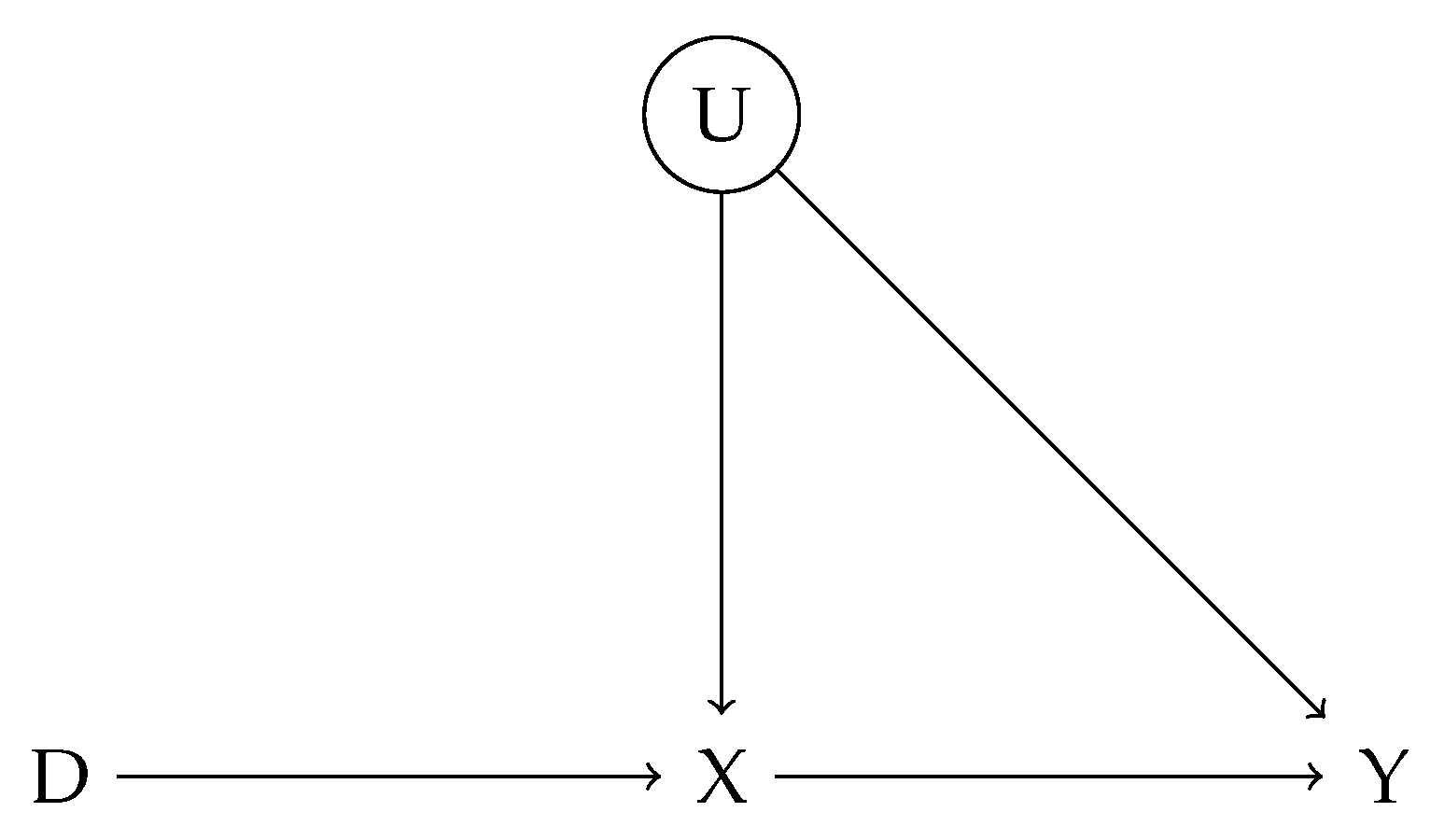
The DAG in Figure 1 depicts a noncompliance experiment in which an unmeasured confounder U simultaneously influences both the treatment variable X and the outcome variable Y. In this model, the instrumental variable D affects whether an individual receives treatment by influencing the treatment variable X, which in turn exerts a direct causal effect on the outcome variable Y.

In addition to the instrumental variable D, the unmeasured confounder U affects both X and Y. This indicates the presence of latent factors that influence both the treatment and outcome, which could introduce bias and complicate the estimation of causal effects. Although the instrumental variable D helps to identify causal relationships, the unmeasured confounder U can bias inferences, particularly when it influences both X and Y but remains uncontrolled.

Therefore, when employing instrumental variable methods for causal inference, particular attention must be paid to the impact of U. Appropriate estimation strategies should be applied to mitigate the influence of unobserved bias on the estimation of causal effects.

We define the causal effect as

$$ACE(X\to Y)=\mathbb{E}\left[Y(x=1)-Y(x=0)\right]=\mathbb{E}\left[Y(x=1)\right]-\mathbb{E}\left[Y(x=0)\right],$$

(1)

where the expectation is given by

$$\begin{array}{cc}\hfill \mathbb{E}\left[Y\right(X=x\left)\right]& =2·P\left\{Y\right(X=x)=2\}+1·P\left\{Y\right(X=x)=1\}+0·P\left\{Y\right(X=x)=0\}\hfill \\ \hfill & =2·P\left\{Y\right(X=x)=2\}+P\left\{Y\right(X=x)=1\}.\hfill \end{array}$$

(2)

Substituting is into the definition of causal effect yields

$$\begin{array}{cc}\hfill ACE(X\to Y)& =\left(2·P\left\{Y\right(X=1)=2\}+P\left\{Y\right(X=1)=1\}\right)\hfill \\ \hfill & -\left(2·P\left\{Y\right(X=0)=2\}+P\left\{Y\right(X=0)=1\}\right).\hfill \end{array}$$

(3)

Equation (3) gives the final expression for the total average causal effect.

3. Novel Bounds

In the setting of Figure 1, D, X, and Y are categorical variables, and both D and X are binary. The possible response patterns of X to D can therefore be classified into four groups: always takers, never takers, compliers, and defiers, as commonly considered in compliance experiments. To formally characterize the response of X to the upstream variable D, we introduce a response-type variable $r_X\in \{0,1,2,3\}$. Each value of $r_X$ represents a deterministic response pattern of X to D under intervention. Specifically, we define a response function $h_{x,r_X}\left(d\right)$, which determines the potential outcome of X given the response type $r_X$ and treatment assignment d:

$$X\left(d\right)=h_{x,r_X}\left(d\right).$$

(4)

The four types are given as follows:

$$h_{x,r_X}\left(d\right)=\left\{\begin{array}{cc}0,\hfill & r_X=0(\mathrm{never}\mathrm{taker}),\hfill \\ 1,\hfill & r_X=1(\mathrm{always}\mathrm{taker}),\hfill \\ d,\hfill & r_X=2\left(\mathrm{complier}\right),\hfill \\ 1-d,\hfill & r_X=3\left(\mathrm{defier}\right).\hfill \end{array}\right.$$

(5)

The corresponding response functions are defined as follows:

$$\begin{array}{c}{h}_{x,0}\left(d\right)=0,d=0,1,h_{x,1}\left(d\right)=1,d=0,1,\hfill \\ h_{x,2}\left(d\right)=\left\{\begin{array}{cc}0,\hfill & \mathrm{if}d=0,\hfill \\ 1,\hfill & \mathrm{if}d=1,\hfill \end{array}\right.h_{x,3}\left(d\right)=\left\{\begin{array}{cc}1,\hfill & \mathrm{if}d=0,\hfill \\ 0,\hfill & \mathrm{if}d=1.\hfill \end{array}\right.\hfill \end{array}$$

(6)

Since the relationship between X and Y is influenced by the unmeasured confounder U, and Y is a trinary variable, this relationship can be categorized into nine classes. Under the linear programming framework proposed by Balke and Pearl [1], classifying the X–Y relationship into nine classes naturally incorporates the effect of the unmeasured confounder U, effectively controlling for confounding and facilitating causal effect analysis. Specifically, the response function of Y depends solely on X, and through this classification, the dependency between X and Y is fully represented by the nine discrete response types.

There are nine possible response types for Y, indexed by $r_Y\in \{0,1,\dots ,8\}$. Each response type corresponds to a deterministic function mapping $X\in \{0,1\}$ to an outcome $Y\in \{0,1,2\}$. We denote this function by $h_{y,r_Y}\left(x\right)$, such that

$$Y\left(x\right)=h_{y,r_Y}\left(x\right).$$

(7)

The response functions corresponding to each response type are defined as follows:

$$\begin{array}{c}{h}_{y,0}\left(x\right)=0,x=0,1,h_{y,1}\left(x\right)=1,x=0,1,h_{y,2}\left(x\right)=2,x=0,1\hfill \\ h_{y,3}\left(x\right)=\left\{\begin{array}{cc}0,\hfill & \mathrm{if}x=0,\hfill \\ 1,\hfill & \mathrm{if}x=1\hfill \end{array}\right.h_{y,4}\left(x\right)=\left\{\begin{array}{cc}0,\hfill & \mathrm{if}x=0,\hfill \\ 2,\hfill & \mathrm{if}x=1\hfill \end{array}\right.h_{y,5}\left(x\right)=\left\{\begin{array}{cc}1,\hfill & \mathrm{if}x=0,\hfill \\ 2,\hfill & \mathrm{if}x=1\hfill \end{array}\right.\\ h_{y,6}\left(x\right)=\left\{\begin{array}{cc}1,\hfill & \mathrm{if}x=0,\hfill \\ 0,\hfill & \mathrm{if}x=1\hfill \end{array}\right.h_{y,7}\left(x\right)=\left\{\begin{array}{cc}2,\hfill & \mathrm{if}x=0,\hfill \\ 0,\hfill & \mathrm{if}x=1\hfill \end{array}\right.h_{y,8}\left(x\right)=\left\{\begin{array}{cc}2,\hfill & \mathrm{if}x=0,\hfill \\ 1,\hfill & \mathrm{if}x=1\hfill \end{array}\right.\end{array}$$

(8)

For notational convenience, we define the shorthand as follows:

$$P_{xy.d}=Pr(X=x,Y=y\mid D=d),x\in \{0,1\},y\in \{0,1,2\},d\in \{0,1\}.$$

(9)

For instance, $P_{11.1}=Pr(X=1,Y=1\mid D=1)$.

3.1. General Bounds for Causal Effects

Theorem 1 presents the complete upper and lower bounds for nonparametric identification under this framework.

Theorem 1.

The sharp and valid bounds for the causal effect $ACE(X\to Y)=\mathbb{E}\left[Y\right(X=1\left)\right]-\mathbb{E}\left[Y\right(X=0\left)\right]$ are given by the following inequality:

$$\mathit{lower}\mathit{bound}\le ACE(X\to Y)\le \mathit{upper}\mathit{bound},$$

(10)

where the lower bound is

$$=max\left\{\begin{array}{c}1+P_{00.0}-2P_{00.1}-2P_{10.1}-3P_{01.1}+2P_{11.0}-4P_{11.1}+P_{02.0}-4P_{02.1},\hfill \\ 1+P_{00.0}-2P_{00.1}-2P_{10.1}-2P_{01.1}+P_{11.0}-3P_{11.1}+P_{02.0}-3P_{02.1},\hfill \\ 1+P_{00.0}-2P_{00.1}-2P_{10.0}-2P_{10.1}-2P_{01.0}-P_{11.0}-3P_{11.1}+P_{02.0}-3P_{02.1},\hfill \\ 1-P_{00.1}-2P_{10.1}-2P_{01.1}+P_{11.0}-3P_{11.1}+P_{02.0}-3P_{02.1},\hfill \\ 1-2P_{00.0}+P_{00.1}-2P_{10.0}-2P_{10.1}-2P_{01.1}-P_{11.0}-3P_{11.1}+P_{02.0}-3P_{02.1},\hfill \\ 1-2P_{00.0}+P_{00.1}-2P_{10.0}-2P_{10.1}-2P_{01.0}-P_{11.0}-3P_{11.1}+P_{02.0}-3P_{02.1},\hfill \\ 1+P_{00.0}-3P_{00.1}+2P_{10.0}-4P_{10.1}-4P_{01.1}+P_{11.0}-3P_{11.1}+P_{02.0}-3P_{02.1},\hfill \\ 1+P_{00.0}-2P_{00.1}+P_{10.0}-3P_{10.1}-3P_{01.1}+2P_{11.0}-4P_{11.1}+P_{02.0}-4P_{02.1},\hfill \\ 1+P_{00.0}-2P_{00.1}+P_{10.0}-3P_{10.1}-3P_{01.1}-2P_{11.1}-2P_{02.1},\hfill \\ 1+P_{00.0}-2P_{00.1}+P_{10.0}-3P_{10.1}-3P_{01.1}-P_{11.0}-P_{11.1}-P_{02.0}-2P_{02.1},\hfill \\ 1+P_{00.0}-2P_{00.1}-2P_{10.0}-2P_{10.1}-2P_{01.0}-P_{11.0}-P_{11.1}-P_{02.0}-P_{02.1},\hfill \\ 1+P_{00.0}-2P_{00.1}-2P_{10.1}-2P_{01.1}-P_{11.0}-P_{11.1}-P_{02.0}-P_{02.1},\hfill \\ 1+P_{00.0}-2P_{00.1}-2P_{10.0}-2P_{10.1}-2P_{01.1}-3P_{11.0}-P_{11.1}-3P_{02.0}+P_{02.1},\hfill \\ 1-2P_{00.0}+P_{00.1}-3P_{10.0}+P_{10.1}-3P_{01.0}-3P_{11.0}+P_{11.1}-3P_{02.0}+P_{02.1},\hfill \\ 1-2P_{00.0}+P_{00.1}-3P_{10.0}+P_{10.1}-3P_{01.0}-4P_{11.0}+2P_{11.1}-4P_{02.0}+P_{02.1},\hfill \\ 1+P_{00.0}-2P_{00.1}-2P_{10.0}-2P_{10.1}-2P_{01.0}-3P_{11.0}-P_{11.1}-3P_{02.0}+P_{02.1},\hfill \\ 1-P_{00.0}-2P_{10.0}-2P_{01.0}-3P_{11.0}+P_{11.1}-3P_{02.0}+P_{02.1},\hfill \\ 1-2P_{00.0}+P_{00.1}-2P_{10.0}-2P_{10.1}-2P_{01.1}-3P_{11.0}-P_{11.1}-3P_{02.0}+P_{02.1},\hfill \\ 1-2P_{00.0}+P_{00.1}-2P_{10.0}-3P_{01.0}-4P_{11.0}+2P_{11.1}-4P_{02.0}+P_{02.1},\hfill \\ 1-2P_{00.0}+P_{00.1}-2P_{10.0}-2P_{01.0}-3P_{11.0}+2P_{11.1}-4P_{02.0}+P_{02.1}.\hfill \end{array}\right.$$

(11)

and the upper bound is

$$=min\left\{\begin{array}{c}4-2P_{00.0}-2P_{10.0}-2P_{10.1}-3P_{01.0}-3P_{11.0}-2P_{02.1},\hfill \\ 2+2P_{00.1}-2P_{10.1}-P_{01.0}+P_{01.1}-3P_{11.0}+2P_{11.1},\hfill \\ 3-P_{00.0}+P_{00.1}-P_{10.0}-2P_{10.1}-2P_{01.0}-3P_{11.0}+P_{11.1}-P_{02.1},\hfill \\ 5-3P_{00.0}-2P_{10.0}-2P_{10.1}-4P_{01.0}-3P_{11.0}-P_{11.1}-3P_{02.1},\hfill \\ 4-2P_{00.1}-2P_{10.0}-2P_{10.1}-3P_{01.0}-P_{11.0}-P_{11.1}-2P_{02.0},\hfill \\ 4-2P_{00.0}-2P_{10.0}-2P_{10.1}-3P_{01.0}-2P_{11.0}-P_{11.1}-2P_{02.1},\hfill \\ 2-2P_{10.1}-P_{01.0}-P_{11.1},\hfill \\ 2+P_{00.1}-2P_{10.1}-P_{01.0}-2P_{11.0}+P_{11.1},\hfill \\ 5-2P_{00.0}-P_{00.1}-2P_{10.0}-2P_{10.1}-4P_{01.0}-3P_{11.0}-P_{11.1}-3P_{02.1},\hfill \\ 2+P_{00.0}+P_{10.0}-3P_{10.1}-P_{01.1}-P_{11.0}+P_{02.0},\hfill \\ 4-P_{00.0}-P_{00.1}-2P_{10.0}-2P_{10.1}-3P_{01.0}-2P_{11.0}-P_{11.1}-2P_{02.1},\hfill \\ 4-2P_{00.1}-2P_{10.0}-2P_{10.1}-3P_{01.0}-P_{11.0}-P_{11.1}-2P_{02.1},\hfill \\ 3-P_{00.1}-P_{10.0}-2P_{10.1}-2P_{01.0}-P_{11.0}-P_{11.1}-P_{02.1},\hfill \\ 4-2P_{00.0}-2P_{10.0}-2P_{10.1}-P_{01.0}-2P_{01.1}-3P_{11.1}-2P_{02.0},\hfill \\ 5-3P_{00.1}-2P_{10.0}-2P_{10.1}-2P_{01.0}-2P_{01.1}-P_{11.0}-3P_{11.1}-3P_{02.0},\hfill \\ 4-2P_{00.0}-2P_{10.0}-2P_{10.1}-P_{01.0}-2P_{01.1}-2P_{11.0}-P_{11.1}-2P_{02.1},\hfill \\ 3-P_{00.0}-P_{10.0}-2P_{10.1}-2P_{01.1}-P_{11.0}-P_{11.1}-P_{02.1},\hfill \\ 2+P_{00.0}-2P_{10.1}-P_{01.1}+P_{11.0}-2P_{11.1},\hfill \\ 2+P_{00.1}-2P_{10.0}-P_{01.0}-2P_{11.0}+P_{11.1},\hfill \\ 3-P_{00.1}-2P_{10.0}-P_{10.1}-2P_{01.0}-P_{11.0}-P_{11.1}-P_{02.0},\hfill \\ 4-2P_{00.1}-2P_{10.0}-2P_{10.1}-2P_{01.0}-P_{01.1}-P_{11.0}-P_{11.1}-2P_{02.1},\hfill \\ 2+P_{00.0}-2P_{10.1}-P_{01.0}+P_{01.1}+P_{11.0}.\hfill \end{array}\right.$$

(12)

These bounds are derived under the assumptions of the causal model illustrated in Figure 1, and are expressed as linear functions of the observed joint distribution $P(X,Y\mid D)$. The lower and upper bounds are sharp, meaning they are the tightest possible given the model and observed data, and are obtained via linear programming over the set of compatible response function distributions. Point identification of the causal effect is generally not possible in this setting due to the presence of unmeasured confounding; however, the bounds provide informative constraints on the average causal effect.

3.2. Causal Effect Bounds Under Monotonicity

Theorem 1 establishes bounds for the causal effect of a binary treatment variable X on an ordinal outcome Y with three levels under general conditions. By further imposing the monotonicity assumption, we obtain the sharp bounds presented in Theorem 2.

Assumption (Monotonicity):

$$X(D=1)\ge X(D=0),$$

(13)

which posits that the treatment variable X is non-decreasing with respect to the instrumental variable D. Specifically, no individual should have a lower probability of receiving the treatment when encouraged by the instrument ($D=1$) than when not encouraged ($D=0$). This excludes individuals whose behavior contradicts the direction of the instrument’s encouragement.

Theorem 2.

Under the additional assumption of monotonicity, the sharp and valid bounds for the causal effect $ACE(X\to Y)=\mathbb{E}\left[Y\right(X=1\left)\right]-\mathbb{E}\left[Y\right(X=0\left)\right]$ are given by the following inequality:

$$\mathit{Lower}\mathit{bound}\le ACE(X\to Y)\le \mathit{Upper}\mathit{bound},$$

where the lower bound is

$$\begin{array}{c}\mathit{Lower}\mathit{bound}=max\{1+P_{00.0}-2P_{00.1}-2P_{10.1}-2P_{01.1}-P_{11.0}-P_{11.1}-P_{02.0}-P_{02.1},\hfill \\ 1+P_{00.0}-2P_{00.1}-2P_{10.1}-2P_{01.1}+P_{11.0}-3P_{11.1}+P_{02.0}-3P_{02.1}\},\hfill \end{array}$$

(14)

and the upper bound is

$$\begin{array}{c}\mathit{Upper}\mathit{bound}=min\{2+2P_{00.0}-2P_{00.1}-2P_{10.1}+P_{01.0}-2P_{01.1}+2P_{11.0}-3P_{11.1},\hfill \\ 2-2P_{10.1}-P_{01.0}-P_{11.1}\}.\hfill \end{array}$$

(15)

Unlike Theorem 1, Theorem 2 incorporates the monotonicity assumption, which excludes defiers, thereby narrowing the set of compliance behaviors and producing sharper bounds on the causal effect. These bounds continue to depend on the observed distribution $P(X,Y\mid D)$ while incorporating this structural constraint.

This analysis leads to two key conclusions. First, without strong assumptions, the nonparametric method yields wider ACE bounds, reflecting greater uncertainty in complex scenarios. Second, introducing monotonicity substantially narrows these bounds, enabling more precise and reliable estimation of the ACE.

4. Simulation Studies

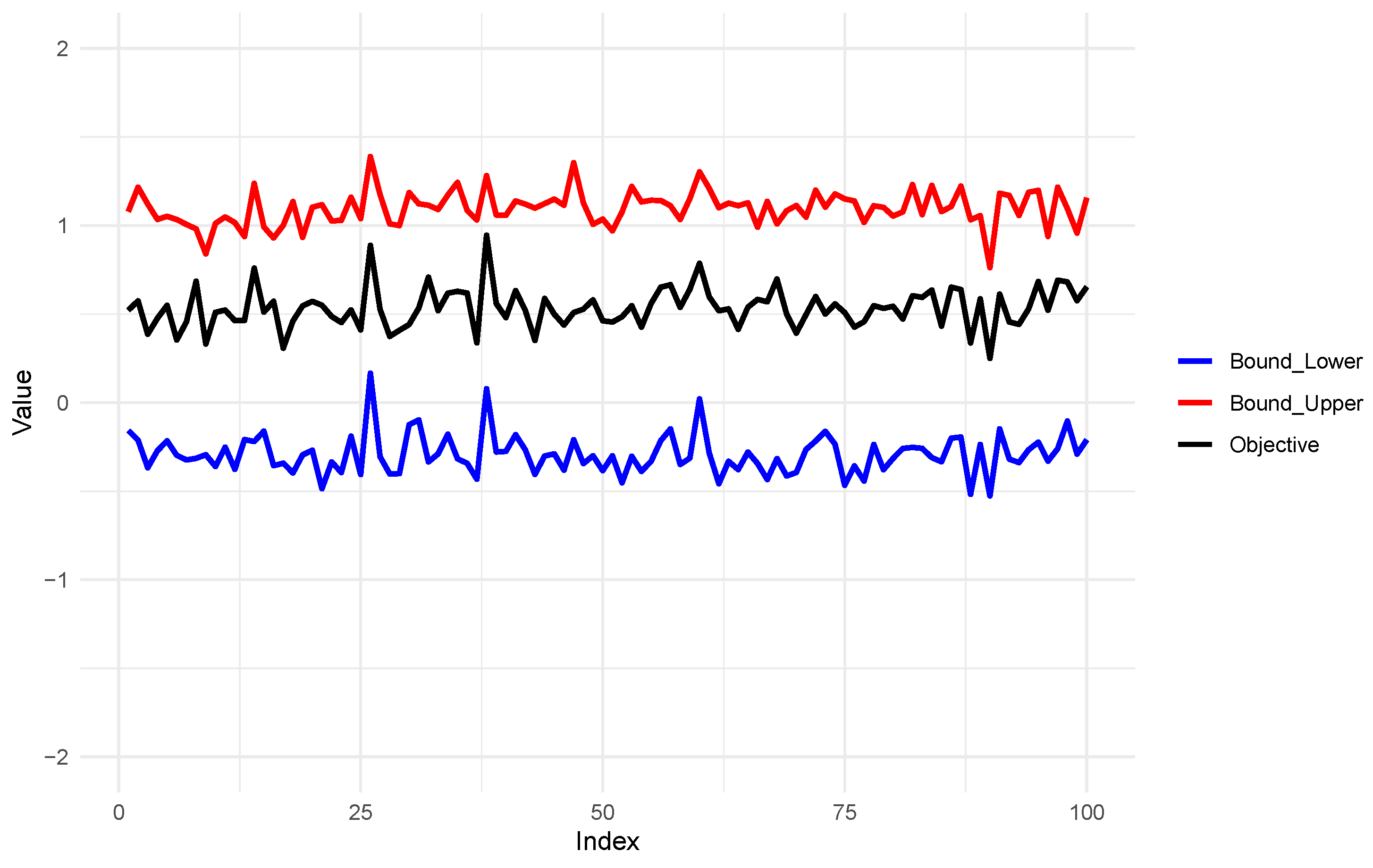
In this section, we validate the ACE bounds derived from Theorems 1 and 2 through numerical simulations to assess the effectiveness of the theoretical results. We plot the true values alongside the upper and lower bounds of the ACE under both theorems and compare the widths of these bounds to visually illustrate how different identifying assumptions affect estimation precision.

First, we assume the following marginal distributions:

$$P(D=1)=0.6,P(U=1)=0.4,P(U=0)=0.6.$$

(16)

A logistic regression model is employed to characterize the conditional distribution of X given D and the unobserved confounder U:

$$Pr(X=1\mid D=d,U=u)=\mathrm{expit}({\alpha }_0+{\alpha }_{D}d+{\alpha }_{U}u+{\alpha }_{DU}du),$$

(17)

where $\mathrm{expit}\left(x\right)=\frac{1}{1+e^{-x}}$. Here, ${\alpha }_0$ denotes the intercept, ${\alpha }_D$ and ${\alpha }_U$ represent the main effects of D and U, respectively, and ${\alpha }_{DU}$ captures their interaction. The coefficients ${\alpha }_0,{\alpha }_D,{\alpha }_U,{\alpha }_{DU}$ are independently drawn from a normal distribution:

$${\alpha }_0,{\alpha }_D,{\alpha }_U,{\alpha }_{DU}\stackrel{\mathrm{i}.\mathrm{i}.\mathrm{d}.}{\sim }\mathcal{N}(1,2).$$

(18)

Then, the conditional distribution of the categorical outcome $Y\in \{0,1,2\}$ is modeled using a multinomial logistic regression with a baseline category. For each category $y\in \{0,1,2\}$, the linear predictor is defined as

$${\eta }_y=b_{0y}+b_{Xy}X+b_{Uy}U,$$

(19)

and the corresponding probability is given by

$$Pr(Y=y\mid X=x,U=u)={\displaystyle \frac{exp\left({\eta }_y\right)}{{\sum }_{j=0}^{2}exp\left({\eta }_j\right)}},$$

(20)

where $b_{0y}$, $b_{Xy}$, and $b_{Uy}$ represent the intercept, the effect of X, and the effect of the unobserved confounder U on the log-odds of outcome $Y=y$, respectively. The coefficients $b_{0y},b_{Xy},b_{Uy}$ are independently drawn from a normal distribution:

$$b_{0y},b_{Xy},b_{Uy}\stackrel{\mathrm{i}.\mathrm{i}.\mathrm{d}.}{\sim }\mathcal{N}(1,1).$$

(21)

Given the specified conditional models for X and Y, we apply the law of total probability to derive the joint distribution $P(Y,X,D)$, from which the conditional distribution $P(X,Y\mid D)$ is obtained.

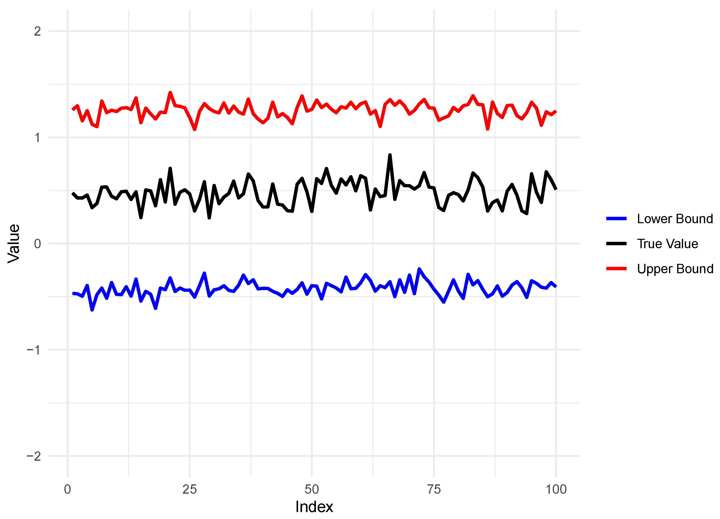
Figure 2 and Figure 3 present the true values along with the upper and lower bounds of the ACE under Theorems 1 and 2, respectively. A comparison between these figures clearly shows that incorporating the monotonicity assumption in Theorem 2 results in substantially narrower bounds, consistent with the theoretical results.

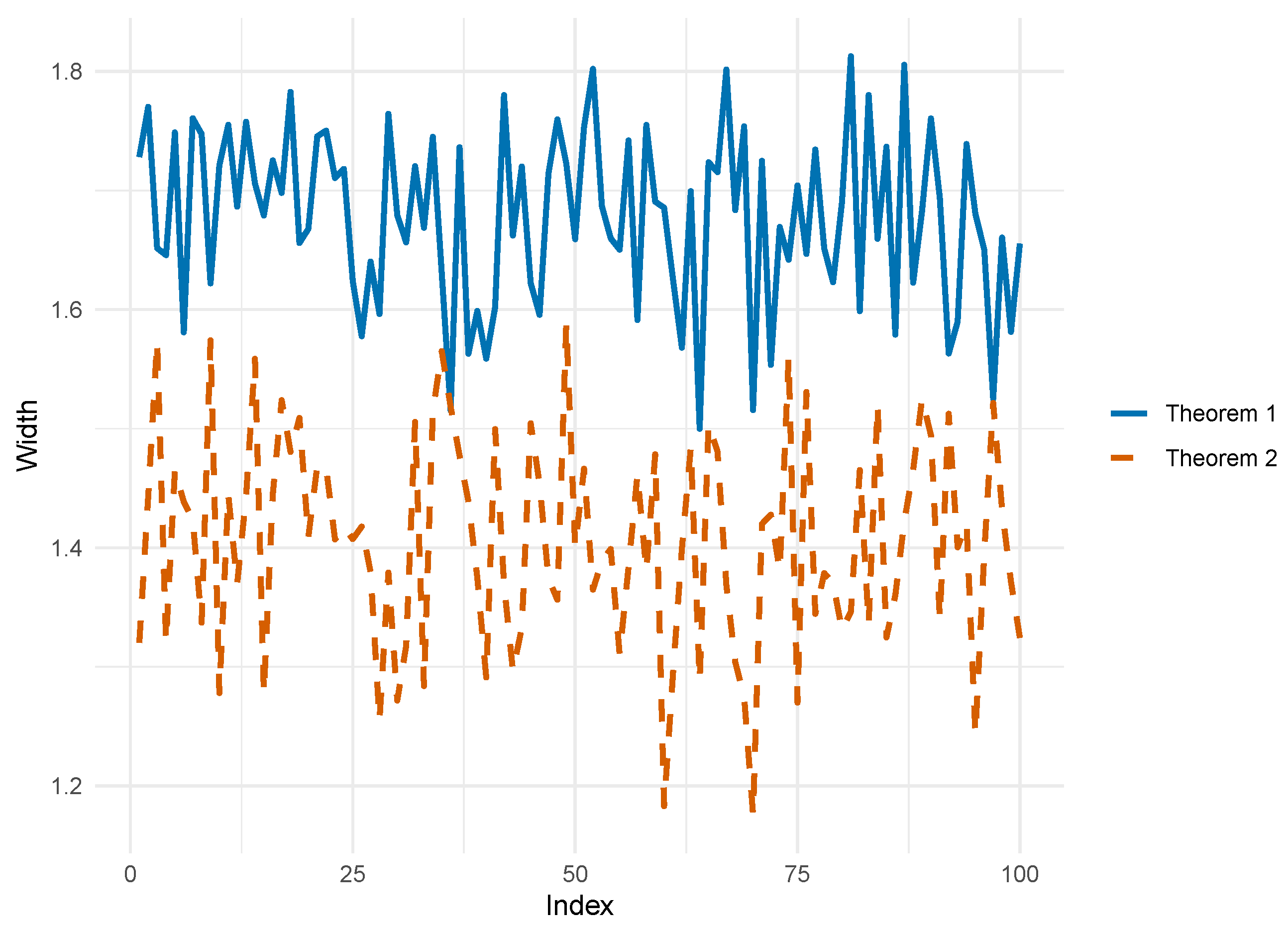
After generating the figures for Theorems 1 and 2, we calculated the widths between the upper and lower bounds. Figure 4 displays these widths based on 100 simulated samples. The horizontal axis represents the sample index, and the vertical axis shows the interval width, computed as the difference between the upper and lower bounds. This figure visually compares the estimation precision and uncertainty of the two methods. We focus on the width of the ACE bounds because, in the presence of unmeasured confounding, it reflects the uncertainty arising from partial identifiability of the model. Our analysis shows that the bounds derived under Theorem 1 are substantially wider than those under Theorem 2. This indicates that relying solely on minimal assumptions leads to considerable uncertainty in ACE estimation, whereas incorporating structural assumptions such as monotonicity in Theorem 2 significantly tightens the bounds. These results demonstrate that additional structural assumptions enhance model identifiability and allow for more precise ACE estimation.

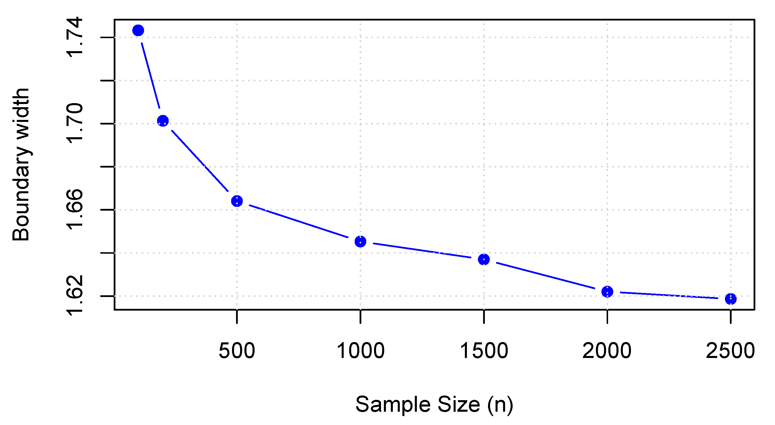
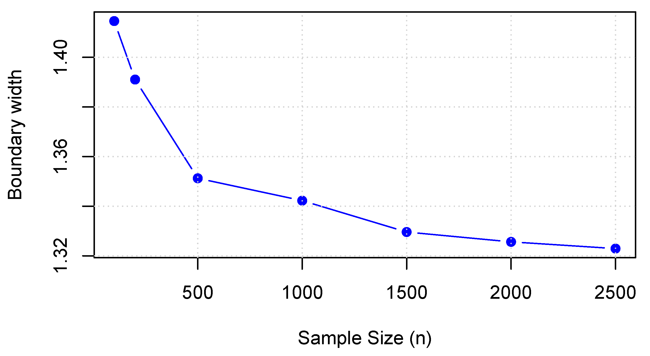
Figure 5 and Figure 6 illustrate the changes in bound width with increasing sample sizes under Theorems 1 and 2, respectively. The results indicate that as the sample size increases, the bound widths gradually shrink and stabilize, demonstrating that the bound estimates exhibit desirable large-sample properties under the corresponding assumptions. In particular, larger sample sizes lead to improved precision of the bound estimates.

5. Real Data Application

This study uses the CDC Diabetes Health Indicators Dataset, which is publicly available on the Kaggle platform (https://www.kaggle.com/datasets/alexteboul/diabetes-health-indicators-dataset, accessed on 16 April 2025).

The dataset originates from the 2015 Behavioral Risk Factor Surveillance System (BRFSS), a program of the CDC in the United States. It contains health-related information on more than 400,000 U.S. adults, covering aspects such as lifestyle behaviors, chronic conditions, and access to healthcare.

The treatment variable X indicates whether an individual has diabetes or pre-diabetes, taking the value 1 if either condition is present and 0 otherwise. The instrumental variable D is constructed as a binary indicator of whether the individual has been diagnosed with high cholesterol. While high cholesterol is associated with an increased risk of diabetes, it is assumed to have no direct effect on self-rated health, making it a valid instrument under standard assumptions. The outcome variable Y represents self-rated health and is categorized into three levels: good health ($Y=0$), average health ($Y=1$), and poor health ($Y=2$).

After cleaning and preprocessing the data, we computed the empirical joint conditional probabilities $P(X,Y\mid D)$ based on the observed values in the dataset.

By substituting the observed values into Theorem 1, we obtain the following bounds for the average causal effect (ACE) of diabetes status X on self-rated health Y:

$$0.596146\le \mathrm{ACE}(X\to Y)\le 1.783746.$$

(22)

The results indicate that diabetes substantially increases the likelihood that individuals will perceive their health status as poor. Since the estimated bounds of the causal effect are strictly positive, regardless of whether conservative or more relaxed identification assumptions are adopted, the influence of diabetes on subjective health perception consistently points in the same deteriorating direction.

From a causal inference perspective, diabetes significantly reduces individuals’ subjective health perception. In other words, individuals with diabetes are more likely to perceive themselves as being in poor health compared to those without diabetes. This negative impact remains robust even after accounting for potential confounders such as BMI, which may simultaneously influence both the risk of diabetes and health perceptions.

6. Conclusions and Discussion

This article investigates the problem of bounding causal effects in the presence of unmeasured confounding, where the treatment variable is binary and the outcome variable is ordinal with three levels. The main contribution is the derivation of general bounds on causal effects for trichotomous outcomes and the further tightening of these bounds through monotonicity assumptions, thereby extending existing results to more general settings.

While this study advances understanding of unmeasured confounding, it also has certain limitations. For ordinal outcomes, increasing the number of levels substantially raises the computational complexity of deriving bounds. Moreover, the bounds obtained under unmeasured confounding are inevitably wide. Future research may focus on optimizing computational methods and exploring strategies to narrow these bounds, such as imposing additional assumptions like monotonicity or leveraging auxiliary information such as proxy variables. These directions would enhance the applicability of our framework to more complex causal models.

References

1. Balke, A.; Pearl, J. Bounds on Treatment Effects from Studies with Imperfect Compliance. J. Am. Stat. Assoc. 1997, 92, 1171–1176. [Google Scholar] [CrossRef]
2. Gabriel, E.E.; Sjölander, A.; Sachs, M.C. Nonparametric Bounds for Causal Effects in Imperfect Randomized Experiments. J. Am. Stat. Assoc. 2023, 118, 684–692. [Google Scholar] [CrossRef]
3. Balke, A.; Pearl, J. Counterfactual Probabilities: Computational Methods, Bounds and Applications. In Uncertainty in Artificial Intelligence; Elsevier: Amsterdam, The Netherlands, 1994; pp. 46–54. [Google Scholar]
4. Horowitz, J.L.; Manski, C.F. Nonparametric Analysis of Randomized Experiments with Missing Covariate and Outcome Data. J. Am. Stat. Assoc. 2000, 95, 77–84. [Google Scholar] [CrossRef]
5. Didelez, V.; Sheehan, N. Mendelian Randomization as an Instrumental Variable Approach to Causal Inference. Stat. Methods Med. Res. 2007, 16, 309–330. [Google Scholar] [CrossRef] [PubMed]
6. Gabriel, E.E.; Sjölander, A.; Follmann, D.; Sachs, M.C. Cross-Direct Effects in Settings with Two Mediators. Biostatistics 2023, 24, 1017–1030. [Google Scholar] [CrossRef] [PubMed]
7. Splawa-Neyman, J.; Dabrowska, D.M.; Speed, T.P. On the application of probability theory to agricultural experiments. Essay on principles. Section 9. Statist. Sci. 1990, 5, 465–472. [Google Scholar] [CrossRef]
8. Rubin, D.B. Estimating Causal Effects of Treatments in Randomized and Nonrandomized Studies. J. Educ. Psychol. 1974, 66, 688. [Google Scholar] [CrossRef]
9. Rosenbaum, P.R. Effects Attributable to Treatment: Inference in Experiments and Observational Studies with a Discrete Pivot. Biometrika 2001, 88, 219–231. [Google Scholar] [CrossRef]
10. Agresti, A.; Kateri, M. Ordinal Probability Effect Measures for Group Comparisons in Multinomial Cumulative Link Models. Biometrics 2017, 73, 214–219. [Google Scholar] [CrossRef] [PubMed]
11. Cheng, J. Estimation and Inference for the Causal Effect of Receiving Treatment on a Multinomial Outcome. Biometrics 2009, 65, 96–103. [Google Scholar] [CrossRef] [PubMed]
12. Huang, E.J.; Fang, E.X.; Hanley, D.F.; Rosenblum, M. Inequality in Treatment Benefits: Can We Determine If a New Treatment Benefits the Many or the Few? Biostatistics 2017, 18, 308–324. [Google Scholar] [CrossRef] [PubMed]
13. Lu, J.; Ding, P.; Dasgupta, T. Treatment Effects on Ordinal Outcomes: Causal Estimands and Sharp Bounds. J. Educ. Behav. Stat. 2018, 43, 540–567. [Google Scholar] [CrossRef]
14. Lu, J.; Zhang, Y.; Ding, P. Sharp Bounds on the Relative Treatment Effect for Ordinal Outcomes. Biometrics 2020, 76, 664–669. [Google Scholar] [CrossRef] [PubMed]
15. Gabriel, E.E.; Sachs, M.C.; Jensen, A.K. Sharp Symbolic Nonparametric Bounds for Measures of Benefit in Observational and Imperfect Randomized Studies with Ordinal Outcomes. Biometrika 2024, 111, 1429–1436. [Google Scholar] [CrossRef]
16. Sun, H.; Shi, C.; Zhao, Q. Bounding the probability of causation under ordinal outcomes. In Communications in Statistics—Theory and Methods; Taylor and Francis: London, UK, 2025; pp. 1–12. [Google Scholar]
Figure 1. Causal diagram with unmeasured confounding.
Mathematics 13 03103 g001
Figure 2. Bounds under Theorem 1.
Mathematics 13 03103 g002
Figure 3. Bounds under Theorem 2.
Mathematics 13 03103 g003
Figure 4. The width of the bounds.
Mathematics 13 03103 g004
Figure 5. Bound width convergence under Theorem 1.
Mathematics 13 03103 g005
Figure 6. Bound width convergence under Theorem 2.
Mathematics 13 03103 g006
Disclaimer/Publisher’s Note: The statements, opinions and data contained in all publications are solely those of the individual author(s) and contributor(s) and not of MDPI and/or the editor(s). MDPI and/or the editor(s) disclaim responsibility for any injury to people or property resulting from any ideas, methods, instructions or products referred to in the content.