Abstract
Rural areas often lack convenient delivery logistics services, which has become a major obstacle to their economic development. Network design initiatives that synergize passenger and freight transport have been identified as effective solutions to address this challenge. Building upon this initiative, this study investigates a novel three-echelon location-routing problem that synergizes trucks and fixed-route buses (3E-LRP-TF). The model is designed with an innovative operational mode that enables fixed-route buses and trucks to travel in a parallel manner, representing a valuable extension to traditional integrated passenger–freight distribution network design. A mixed-integer nonlinear programming model with the objective of minimizing the total network cost is constructed to formulate the problem. Furthermore, a bottom-up three-phase adaptive large neighborhood search (ALNS) algorithm is designed to solve the problem. A final empirical study was conducted, with Qingchuan County in China serving as a case study, with the aim of validating the effectiveness of the proposed model and algorithm. The results show that, compared with using trucks alone, the synergistic network system has the potential to reduce costs by more than 5% for parcel pickup and delivery services. The proposed algorithm can address larger-scale problems and exhibits better performance with regard to solution quality and efficiency. Sensitivity analysis indicates that the parcel transport capacity of bus routes exerts a nonlinear effect on total costs, and changes in service radius result in trade-offs between cost and accessibility. These findings provide actionable insights for policymakers and logistics operators.
Keywords:
integration of passenger and freight transport; three-echelon location-routing problem; three-phase ALNS algorithm; collection and delivery points; service radius; rural delivery logistics MSC:
90B06; 90C27
1. Introduction
As rural e-commerce has grown exponentially in recent years, rural delivery logistics has become one of the pivotal channels through which agricultural products from farms are distributed to urban areas and products from cities are delivered to rural regions, playing a significant role in promoting rural agricultural development and rural revitalization [1,2,3,4]. For instance, the volume of parcels delivered and collected in rural areas of China amounted to 37 billion in 2021, thereby facilitating and propelling the movement of agricultural products into cities and industrial goods into rural areas, generating over CNY 1.85 trillion in revenue [5]. However, despite these substantial volumes, the low population density means that courier, express, and parcel service providers (CSPs) must carry relatively few packages across wide expanses of land, resulting in high per-unit delivery costs and limited economies of scale [6,7,8]. Consequently, many commercial CSPs show little willingness to deeply engage in rural markets, resulting in a lack of efficient and cheap services for express package delivery, which further generates negative feedback effects and widens the urban–rural gap [9]. Therefore, innovative solutions to bottleneck issues are crucial and worthy of careful consideration.
The prevailing consensus among researchers and entrepreneurs is that a hybrid network integrating passenger and freight transport constitutes a promising option. Integrated passenger and freight transport (IPFT) was first proposed in the “Green Paper on Urban Transport” released by the European Commission in 2007, which specifically tells us to “consider all urban logistics related to passenger and freight transport together as a single logistics system” [10]. In recent years, IPFT has undergone continuous expansion and application in rural areas across various countries. Positive feedback has been demonstrated to include reduced vehicle mileage and fuel consumption, improved service coverage, freight delivery volume, and passenger vehicle occupancy rates [11,12,13,14,15,16,17]. In China, IPFT has already become one of the main solutions for the development of delivery logistics in rural areas. According to data from the Ministry of Transport of the People’s Republic of China, more than 1100 counties in China had launched IPFT services in rural areas by the end of 2023, with over 200 million parcels delivered by buses [18]. Our study is conducted in the context of encouraging hybrid services, aiming to provide valuable references for how to develop synergistic network.
According to our knowledge, the main modes involved in current research and practice in rural areas are share-a-ride (SAR) and freight on transit (FOT) [15,17,19]. For SAR mode, door-to-door transportation services for passengers and cargo are provided by demand-responsive rural buses, which are associated with high service costs. For FOT mode, goods are first transported to a transfer station and then delivered to customers by other vehicles. However, the process is strictly constrained by bus schedules, which can result in significant challenges related to flexibility and implementation.
In response to the issues identified in the above modes, we propose a new FOT type in which fixed-route buses and trucks operate in a parallel manner and are integrated into the design of the three-echelon rural delivery logistics network. The network consists of one distribution center (DC), several distribution stations (DSs), collection and delivery points (CDPs), and customers, with trucks and fixed-route buses operating on the network. For a subnetwork made up of the DC and DSs, small trucks are used to deliver and pick up parcels. For a subnetwork made up of the DSs and CDPs, buses are considered a type of special truck with fixed routes and stops and are used together with mini-trucks to deliver and pick up parcels. For a subnetwork made up of the CDPs and customers, each customer is assigned a unique CDP for self-service.
Our main contributions are as follows: Firstly, we have established a new 3E-LRP-TF model for designing rural delivery logistics networks that considers the parallel operation of trucks and fixed-route buses. Secondly, a three-phase ALNS algorithm was designed based on the three-echelon network characteristics, using a bottom-up approach to solve the problem associated with each subnetwork. Finally, a case study demonstrates the effectiveness of the model and algorithm and explores some valuable management applications.
The remainder of the paper is organized as follows. Section 2 provides a literature review of related work. Section 3 introduces the formulation of 3E-LRP-TF, followed by the proposed three-phase ALNS algorithm in Section 4. Section 5 reports the results of the case study. The conclusions and future research directions are presented in Section 6.
2. Literature Review
Rural delivery logistics is the critical link connecting cities and rural areas, acting as one of the key channels for bringing agricultural products to urban markets and delivering consumer goods to rural communities. Currently, a unified consensus has emerged regarding rural delivery logistics: it represents the overlapping interaction between rural logistics and delivery logistics in terms of specific service recipients, service areas, and service segments. The focus lies on the collection, sorting, transportation, and delivery of letters, parcels, printed materials, and other items in rural areas. Related studies and practices also involve similar terms such as rural postal logistics, rural express delivery, rural E-grocery logistics, and rural e-commerce logistics [9,20,21,22].
One of the core themes within the aforementioned scope of studies is to systematically identify and analyze their unique characteristics and practical challenges. The prevailing view is that the operational context of rural delivery logistics presents fundamental differences compared to urban FLM distribution. These unique challenges stem primarily from several interrelated factors, including the following: dispersed residential settlements lead to fragmented demand distribution and increased distribution distances; a small population size and limited purchasing power result in lower demand scales; and underdeveloped road infrastructure increases transportation distances [7,9,17,23]. These practical contexts collectively lead to substantially elevated operating costs and severe limitations to achieving economies of scale. Consequently, many commercial CSPs are also reluctant to increase the density of service stations in rural markets and provide timely delivery services, making it difficult for customers in rural areas to access efficient and affordable parcel delivery services. Taking the US as an example, the average distance between two stations in last-mile delivery routes for low-density areas reaches 5–20 miles, whereas the value for urban areas is only 0.2–2 km [24]. A similar observation holds for the Seine-et-Marne region in France, where rural and suburban residents spend an average of 8 min driving to the nearest pickup point—twice the time required in urban areas [25].
To address these challenges, academia and industry have explored and designed some innovative solutions. Among all the proposals, reconfiguring picking locations and reconfiguring transportation are the two core themes concerning the operational model for last-mile fulfillment [7]. In terms of reconfiguring picking locations, existing studies have predominantly framed the question as a multi-echelon network design problem. For example, Yang et al. [26] and Dai et al. [27] developed the two-echelon delivery network incorporating self-pickup points for home delivery and customer pickup service modes, focusing, respectively, on the factors of customer pickup radius constraints and customer satisfaction. Sun et al. [28] further integrated customer self-pickup with service frequency to construct a two-echelon periodic location-routing problem model with flexible service time decisions for network design. Zhang et al. [29] combined collaborative distribution with delivery options to investigate the design problem of three-echelon collaborative distribution networks incorporating CDPs. In terms of reconfiguring transportation, the primary focus is on innovatively integrating transportation resources from different modes or different actors. More frequently mentioned topics include the IPFT, the hybrid truck–drone delivery, the cooperation among multiple logistics providers, and the collaboration of delivery and sale [9,30,31,32]. Given that our topic is about IPFT, we will next provide a detailed review of this field. Readers interested in the other topics mentioned above can consult the corresponding references.
IPFT improves transportation efficiency and resource utilization by combining transportation services for passengers and freight. As IPFT has been implemented at different times and in different countries, the same concept is known by various names, including integrated passenger and freight logistics, collaborative passenger and freight transport, systems with mixed passengers and goods, integrated people and freight transportation, co-modality, cargo hitching, and share-a-ride [33,34,35].
Recent literature reviews indicate that there is growing interest within the scientific community in the operational organization of such hybrid systems, with integration forms involving roads, nodes, and vehicles already being considered [13,33]. Regarding research subjects, it has been expanded from long-distance transportation to “first-last mile” distribution, and from urban areas to rural areas [12,33,34]. IPFT has long been common practice in long-distance transportation, for example, using aircraft cargo holds, long-distance bus luggage compartments, and train luggage racks to carry cargo. At the beginning of the 21st century, IPFT in “first-last mile” distribution began to attract the attention of academia and government departments [9]. Extensive research and practical experience in urban areas have demonstrated the significant sustainability benefits of these hybrid transportation systems, including reducing pollution, noise, traffic congestion, accidents, and operating costs [14,33,36]. In recent years, research has expanded to rural areas with small-scale and scattered demand for both passenger and freight transport, and it has been found to reduce logistics costs and generate additional revenue for public transport operators [13,15,17,37]. However, research into network optimization in rural areas has mostly focused on modeling and optimization under SAR and FOT, influenced by passenger transport types [19].
Most studies related to the SAR mode utilize public transport vehicles without fixed routes, such as taxis and demand-responsive buses, to provide door-to-door services for passengers and packages. It is therefore characterized as a variant of the classical vehicle routing problem. For example, Li et al. [38] studied the SAR problem of people and parcels being handled in an integrated manner by the same taxi network based on the Dial-a-Ride model. Lu et al. [39] investigated the issue of combining passenger and parcel transportation in a mixed fleet of electric and petrol taxis. Their aim was to generate optimal transportation routes for both passenger and parcel delivery demand. He et al. [15] studied an integrated rural public transport system combining passenger and parcel delivery services. They found that the proposed system could achieve annual savings of 66,000 km and USD 21,000 in the case study area. Subsequently, He and Guan [40] conducted further research into the two-echelon vehicle routing problem under incentive policies for IPFT, and found that adequate rewards are conducive to improving the service quality of collaborative systems. However, some studies have also highlighted typical issues that arise when implementing the model in rural areas. For example, Feng et al. [41] assessed the feasibility of implementing IPFT in rural areas in terms of profit and labor. The results indicated that an excessive number of passengers would lead to a shortage of drivers, making the IPFT system unfeasible. Yang et al. [42] conducted a study in Longkou County, Shandong Province, and concluded that the SAR model is better suited to passengers with relatively low time sensitivity, as well as to areas or times of day with low demand.
Studies on the FOT mode have mostly adopted the strategy of connecting public transportation with last-mile distribution. Specifically, public transport vehicles are used to carry cargo along passenger routes, while other vehicles deliver cargo from stations to customers or pickup points. Masson et al. [43] designed an innovative goods delivery system in which goods are first transported from the distribution center to bus stations using spare bus capacity, and then distributed to end users by city freighters. Schmidt et al. [44] modeled the problem as a two-echelon vehicle routing problem involving intermediate stops and conducted extensive computational studies on various possible scenarios and objectives, as well as different instance sets with various demand distributions. Azcuy et al. [45] focused on determining which bus stops are most suitable for use as transfer points, aiming to better understand the impact of transfer location decisions on the system’s operational performance. Furthermore, Sun et al. [17] integrated parcel transportation by bus with simultaneous home delivery and customer self-pickup. Packages are first transported by bus to a bus transfer point and then delivered to a pickup point using small delivery vehicles. Wang et al. [46] conducted further research into the coordinated delivery system involving buses, electric vehicles, and drones, which aims to dynamically match buses and transfer points according to passenger demand. Recently, Delle Donne et al. [47] presented a coordinated three-tier distribution system. First, trucks transport packages from distribution centers to public transport hubs. Then, buses deliver the packages to bus stations. Finally, zero-emission vehicles collect the packages from the stations and deliver them to customers.
The literature review indicates that previous studies have mainly focused on two areas: (1) vehicle routing problems based on SAR mode and (2) network design for the integration of fixed-route transport vehicles with other vehicles. However, these studies did not consider the option of operating fixed-route buses and trucks in a parallel manner. Therefore, our work is an extension of and supplement to existing research on IPFT.
3. Optimization Model
3.1. Problem Statement
The 3E-LRP-TF model for designing rural logistics networks is inspired by a real-world application, in which CSPs provide parcel delivery and collection services to rural residents through a three-echelon network comprising a DC, DSs, and CDPs (as shown in Figure 1). The first echelon is a self-pickup network composed of villages and CDPs. The second echelon is a synergistic distribution network composed of CDPs and DSs, using mini-trucks and fixed-route buses. The third echelon is a small truck distribution network composed of DSs and DCs. Decisions to be made include the location of CDPs and their service relationship with customers, the location of DSs and their service relationship with CDPs, mini-truck routes and service buses, and small truck routes, with the objective of minimizing the total network cost.
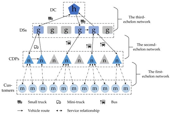
Figure 1.
Network structure diagram of 3E-LRP-TF.
To more clearly illustrate the operational logic of the 3E-LRP-TF network, we present an illustrative example that includes 1 DC, 5 potential DSs, 13 CDPs, and several demand points (as shown in Figure 2). In this case, the CDPs are selected from the demand points. Six of the CDPs rely on bus stops and provide pickup and delivery services by bus, while the others are served by mini-trucks. Two small trucks depart from the DC, delivering parcels to three opened DSs while simultaneously picking up parcels. Then, parcels to be delivered are further transported by two bus schedules and three mini-trucks to the opened CDPs, where customers utilize self-pickup at the corresponding CDP. In reverse, parcels sent by customers via CDP are collected by bus or mini-truck to an opened DS, and then transported by small truck to the DC.
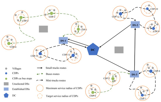
Figure 2.
Illustrative example of the 3E-LRP-TF.
The following assumptions have been made regarding the model, given the actual practices of rural delivery logistics and bus operations:
- (1)
- Each CDP can only be served by one DS, and each village can only be assigned to one CDP.
- (2)
- Trucks, buses, DSs, and CDPs have capacity restrictions.
- (3)
- As the origin and destination of buses often differ in real-world scenarios, it is not possible for the same bus to provide simultaneous pickup and delivery services for the same CDP.
- (4)
- In FLM distribution scenarios, CSPs typically define a relatively stable geographical service range for CDPs to ensure operational efficiency and service quality. We therefore implemented service area restrictions for CDPs in line with the initiatives proposed by existing practices and studies [17,26,27]. CDPs cannot provide services to customers outside their maximum service radius; penalties are incurred if CDPs provide services to villages outside the target service radius.
- (5)
- Buses should be equipped with separate, enclosed compartments for storing parcels, as is commonly practiced in IPFT. For example, in China and Sweden, the physical separation of parcels from passengers (such as through the use of onboard parcel lockers or luggage compartments) is a prerequisite for implementing mixed transportation, which also ensures safety [15].
- (6)
- A centralized decision maker (i.e., a comprehensive service platform for IPFT) coordinates bus schedules with parcel shipments and ensures that parcel loading/unloading operations are completed within the bus dwell time at stops.
- (7)
- For security purposes, parcels must be in the permitted categories (such as small lightweight necessities and agricultural products) and undergo security checks.
Table 1 summarizes the notation used in the model’s formulation.

Table 1.
Sets, parameters, and decision variables.
3.2. Mathematical Model
According to the above problem description and symbol definitions, the 3E-LRP-TF model is formulated with the objective of minimizing the total network cost. The total network cost comprises the fixed usage costs of facilities and vehicles, vehicle transport costs, bus conversion costs, bus route usage costs, and self-service penalty costs, calculated as shown in Equation (1):
The problem corresponding to the first-echelon network is a location-allocation problem, requiring decisions on the location of CDPs and their service relationship with customers. It is specifically defined by the Equations (2)–(10):
Constraint (2) ensures that each village can only be assigned to one CDP. Constraint (3) specifies that only opened CDPs will provide services to the village. Constraint (4) represents the maximum service radius limitation of the CDP. Constraints (5) and (6) determine whether the self-service radius for village demand is less than or equal to . Constraints (7) and (8) provide the calculations for the volume of parcels to be picked up and delivered if CDP . Constraint (9) specifies the capacity of the CDP. Constraints (10) and (11) define the domains of decision variables.
Once the determined CDPs are input into the second-echelon network, we can characterize the problem of this echelon as a location-route problem. Therefore, decisions need only be made for the location of DSs and their service relationship with CDPs, mini-truck routes, and service buses. It can be formulated as Equations (12)–(66):
Constraints (12) and (13) ensure that an open CDP must be served by one open DS. Constraint (14) ensures that no mini-truck routes are generated between two DSs. Constraint (15) aims to eliminate symmetric solutions. Constraint (16) ensures that each mini-truck can have at most one service route. Constraints (17) and (18) ensure that only opened CDPs are provided with services. Constraint (19) ensures that each potential CDP is visited at most once by the same vehicle. Constraints (20) and (21) ensure that only opened DSs can provide services to CDPs. Constraint (22) ensures that, if a vehicle passes through a node, it must enter and leave that node. Constraints (23) to (25) ensure that only bus routes and their schedules that connect CDPs and DSs can be used for parcel transportation. Constraint (26) specifies whether CDP can be served by schedule of route . Constraints (27) and (28) specify that, when schedule is used for parcel transportation, it must pass through both the opened DS and CDP. Constraints (29) and (30) specify that, when CDP and DS are connected by the same bus route, must be assigned to . Constraints (31) and (32) stipulate that mini-trucks with an unopened DS cannot visit CDPs. Constraint (33) is the travel distance limit for mini-trucks. Constraints (34) and (35) indicate that only when CDP is served by DS can the route of mini-truck pass through both nodes. Constraints (36) and (37) provide the calculations for the DS pickup delivery demand. Constraint (38) specifies the maximum capacity of the DS. Constraints (39)–(45) specify the maximum capacity of the vehicles. Constraints (46)–(49) are flow conservation constraints for pickup and delivery demand, respectively. Constraint (50) provides the calculation of . Constraint (51) ensures that the pickup load must be equal to zero when the mini-truck departs the DS. Constraint (52) ensures that the total pickup load entering each opened DS equals the total pickup demand of the CDPs assigned to the corresponding DS. Constraint (53) ensures that the total delivery load dispatched from each opened DS equals the total delivery demand of the CDPs assigned to the corresponding DS. Constraint (51) ensures that the delivery load must be equal to zero when the mini-truck returns to the DS. Constraints (55) and (66) define the domains of decision variables.
When the determined DSs are input into the third-echelon network, we can characterize the problem of this echelon as a vehicle path problem. Therefore, small truck routes are a major item on the decision-making table. This problem can be modeled using Equations (67)–(91):
Constraint (67) guarantees that opened DSs must be assigned to a DC. Constraint (68) ensures that each small truck is used at most once. Constraint (69) aims to eliminate symmetric solutions. Constraints (70)–(72) indicate that only opened DSs have unique vehicle entry and departure. Constraint (73) is the maximum travel distance limit for small trucks. Constraints (74) and (75) ensure that the route of small truck can connect the two only if a DS is assigned to the DC. Constraints (76)–(78) are maximum capacity restrictions for small trucks. Constraints (79) and (80) are flow conservation constraints for pickup and delivery demand, respectively. Constraint (81) ensures that the pickup load must be equal to zero when the small truck departs the DC. Constraint (82) ensures that the total pickup load entering DC equals the total pickup demand of the opened DSs. Constraint (83) ensures that the total delivery load dispatched from the DC is equal to the total delivery demand of the opened DSs. Constraint (84) ensures that the delivery load must be equal to zero when the small truck returns to the DC. Constraints (85)–(91) define the domains of decision variables.
4. Three-Phase ALNS Algorithm
It is extremely difficult to solve the 3E-LRP-TF problem because it is a variant of the multi-echelon location-routing problem [48,49]. It is also mostly infeasible to solve the problem using an exact algorithm in a reasonable amount of time. Inspired by the bottom-up approach in existing algorithms for solving multi-tier network design problems [50,51], a three-phase ALNS algorithm is designed based on the three-echelon network characteristics, using a bottom-up approach to solve the problem associated with each subnetwork. The adaptive mechanism of the algorithm manifests primarily in two aspects. First, it achieves adaptive operator selection by dynamically adjusting the probability of each operator through a roulette wheel selection process. Second, it enables adaptive solution acceptance by introducing an acceptance criterion based on simulated annealing. A flow chart of the three-phase ALNS algorithm is shown in Figure 3.
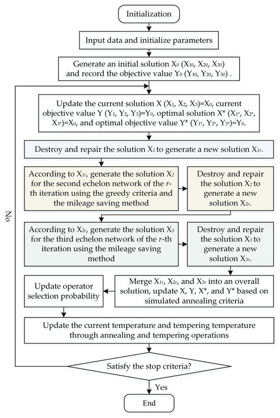
Figure 3.
Flow chart of three-phase ALNS algorithm.
Specifically, we first generate high-quality initial feasible solutions with a three-echelon encoding structure using the designed initial solution construction method. Next, we sequentially solve the location-allocation problem for the first-echelon network, the locating–routing problem for the second-echelon network with simultaneous delivery and pickup, and the vehicle routing problem for simultaneous pickup and delivery in the third-echelon network. Throughout this process, new solutions are generated by destroying and repairing the current solution. Then, the current solution and the optimal solution are updated according to the acceptance criteria of the simulated annealing algorithm. The selection probabilities of the corresponding operators are updated based on the quality of the neighborhood solutions. If the stopping criteria are satisfied, the solution is output as the final result. There are three stopping criteria for iteration: (1) The iteration count reaches the preset maximum value. (2) The solution time reaches the preset maximum value. (3) The tempering temperature drops to the preset temperature. Otherwise, the iteration process is repeated.
4.1. Three-Echelon Encoding Method
The solution is made up of a three-echelon structure of natural number encoding. First-echelon coding corresponds to the self-pickup network, which represents the location of CDPs and their service relationship with customers. It consists of demand points, represented by , and potential CDPs, represented by . Second-echelon coding corresponds to the synergistic distribution network, which represents the location of DSs and the sequential services of mini-trucks and buses to CDPs. It consists of DSs represented by , bus routes and their schedules represented by , opened CDPs, and virtual zero. Third-echelon coding corresponds to the small truck distribution network, which represents the routes traveled by small trucks. It consists of DC, opened DSs, and virtual zero. Note that the introduction of a virtual zero indicates the end of a truck or bus route.
Figure 4 shows a feasible solution comprising 21 demand points, 21 potential CDPs, 5 potential DSs, 1 DC and 3 bus routes. In the first echelon, 22, 23, 28, 32, 33, 36, 39, and 40 are chosen as CDPs, and the numbers following them represent the customers served. For example, CDP 22 serves customers 1, 9, and 13, whereas CDP 28 serves customers 3 and 7. In the second echelon, DSs 43, 44, 45, and 46 are chosen, and the subsequent numbers show the CDPs served by mini-trucks or buses. For example, DS 43 uses bus route 51, schedule 2, to serve CDPs 33 and 36, while DS 44 uses a mini-truck to serve CDPs 39 and 40. In the third echelon, DC 48 employs a small truck to serve DSs 46, 45, 44, and 43 in sequence.
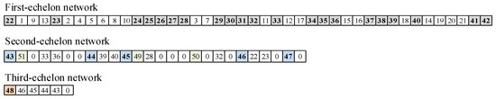
Figure 4.
Example of the three-echelon encoding method.
4.2. Initial Solution Construction
High-quality initial solutions can significantly improve the convergence of the algorithm. Therefore, we use the greedy criterion and the mileage-saving method to generate initial solutions for the three subnetwork problems. Specifically, the greed principle is primarily employed for facility location and service relationship allocation, whereas the mileage-saving method is used to generate the truck routes.
The following greedy criteria are applied to generate the initial solution for the first-echelon network. Specifically, customers will be prioritized for allocation to bus stops that are potential CDPs because it is cheaper to transport parcels by bus. If the parcel pickup and delivery demands cannot be fulfilled by bus stops, customers will be assigned to potential CDPs that are not bus stops. The steps are as follows. (1) Let be the set of potential CDPs that are not bus stops, and let be the number of unassigned customers within the maximum service radius of CDP . (2) Open the CDPs from one by one. The order in which they are opened depends on their value: CDPs with higher values are given priority. If two or more CDPs have the same value, one of them will be selected at random for opening. Subject to capacity limits, customers are assigned to opened CDPs in order of proximity, from the closest to the furthest. If no customer can be assigned to the currently open CDP, it will be removed from . Continue repeating the above assignment process until either becomes empty or all customers have been assigned. (3) If is empty, perform the process in Step (2) on the CDPs in , one by one, until all customers have been assigned.
For the initial solution for the second-echelon network, we prioritize using bus stops as DSs and using buses to transport parcels. Only when bus stops and routes are unavailable should other potential DSs be considered and mini-trucks used to transport parcels. Unlike the assignment process in the first echelon, we prioritize allocating distant CDPs to DSs that act as bus stops. This approach is used to avoid these CDPs being served by mini-trucks, as these incur higher route costs. The steps are as follows. (1) Let be the set of already opened CDPs, be the set of routes passing through , be the set of potential DSs in , be the set of potential DSs excluding , and be the number of CDPs that may be assigned to DS according to the proximity principle. (2) Open the DSs from one by one. The order in which they are opened depends on their value: DSs with higher values are given priority. If two or more DSs have the same value, one of them will be selected at random for opening. Subject to capacity limits, CDPs are assigned to an opened DS in order of distance, from the furthest away to the closest. If no CDP can be assigned to the currently opened DS, it will be removed from . Continue repeating the above assignment process until either becomes empty or all opened CDPs have been assigned. (3) For each CDP assigned to a DS in Step (2), it is necessary to choose the bus schedule for transporting parcels based on capacity restrictions. We match CDPs with bus schedules based on their demand, from highest to lowest, and we prioritize schedules that have already been used. When the capacity of all used schedules cannot meet the CDP’s demand, new bus schedules can be added to provide service. Repeat the process until there are no more schedules available or all opened CDPs have been assigned. (4) If is empty, then open the DSs from one by one. The order in which they are opened depends on their value: DSs with higher values are given priority. If two or more DSs have the same value, the DS closer to the DC is chosen to be opened. If no CDP can be assigned to the currently opened DS, it will be removed from . Repeat the process until all CDPs are assigned to DSs. Finally, the route for the mini-trucks is generated using the mileage-saving method.
For the initial solution for the third-echelon network, the mileage-saving method is used to generate the service route for small trucks.
4.3. Destroy and Repair Operators
The ALNS algorithm improves solution quality continuously through destroy and repair operations. In our work, we develop 14 destroy operators and 7 repair operators customized to the features of the problem. Since the operators used to solve the three subproblems are quite similar, the designed operators are presented solely from the perspective of the second-echelon network to avoid repetition. When the operators described below are applied to solve a first-echelon network, CDP should be replaced with a demand point, DS should be replaced with CDP, and bus route and mini-truck elements must be removed. When applied to a third-echelon network, CDP should be replaced with DS, DS should be replaced with DC, mini-truck should be replaced with small truck, and the content related to bus routes must be removed.
4.3.1. Destroy Operators
As shown in Table 2, the destroy operators are primarily used to modify node locations, allocation relationships, and routing. Operators (1), (2), (4)–(8), and (14) are used for the first-echelon network; operators (1)–(13) are used for the second-echelon network; and operators (4)–(11) are used for the third-echelon network.
Table 2.
The 14 designed destroy operators.
The usage rate of DS in the worst DS removal operator is calculated as shown in Equation (92):
The calculation of similarity in the improved Shaw removal operator is shown in Equation (93). The smaller is, the more similar node is to node . represents the distance between node and node . indicates the similarity between the delivery and pickup volumes of node and node . If node and node are connected by a bus route, then equals 1; otherwise, it equals 0. represent the weights of the corresponding items.
The calculation of the cost change value in the maximum route cost change removal operator is presented in Equations (94)–(98). Equation (94) shows the calculation of the change in truck route cost value . Equations (95)–(98) correspond to the changes in bus route cost value under four different scenarios. Of these, Equation (95) corresponds to the scenario with no changes; Equation (96) to the scenario with a decrease in the number of bus schedules only; Equation (97) to the scenario with a decrease in both the number of bus routes and schedules; and Equation (98) to the scenario with a decrease in the number of DSs, bus routes, and schedules. In the formula, represents the set of opened CDPs. represents the route to the CDP. represent the predecessor and successor nodes of the CDP . represents the distance between nodes and . represents the perturbation factor, which has a value between 0.8 and 1.2:
The calculation of the extreme degree in the extreme CDP removal operator is presented in Equations (99) and (100). represents the set of mini-truck routes among feasible solutions. represents the routes in set . represents the average distance between two neighboring CDPs in route .
The calculation of in the small truck route removal operator is presented in Equation (101):
4.3.2. Repair Operators
In total, seven repair operators are designed for use, of which operators (1) and (2) are used for the first-echelon network, and operators (3)–(7) are used for the second- and third-echelon networks.
- (1)
- Penalty costs greedy insertion
This operator is designed to minimize the penalty cost of self-service. The CDP with the highest number of customers within the target service radius will be given priority. If there are multiple CDPs within that have the same number of customers, then the CDP with the largest number of customers within the maximum coverage radius is selected. Going further, if there are multiple CDPs within that have the same number of customers, priority will be given to the CDP with the smallest total self-service distance.
- (2)
- Facility utilization greedy insertion
This operator is designed to maximize CDP utilization. When opened CDPs are sufficient to meet customer demand, insertion is performed according to the principle of maximum capacity utilization. If the opened CDPs are insufficient to meet demand, the same operation is performed as for penalty costs greedy insertion, based on the relationship between distance and .
- (3)
- Basic greedy insertion
This operator is designed to minimize route cost changes after CDP insertion. Under the restrictions of truck capacity, bus schedule capacity, and DS capacity, we first calculate the changes in the objective function and after inserting the CDP into the optimal mini-truck route and bus route using Equations (94)–(98). Then, the contribution of CDP to the objective function value is calculated using Equation (102), and the CDP with the smallest is inserted into the corresponding truck or bus route. represents the set of CDPs to be inserted:
- (4)
- Greedy insertion perturbation
This operator increases the diversity of solutions by introducing noise terms and randomization to basic greedy insertion. Without violating the capacity restriction, the change in the objective function after inserting CDP is calculated according to Equation (99), and the CDP with the smallest is selected for insertion. The noise term is denoted by . The noise level is controlled by a parameter B, which is a random number in the interval :
- (5)
- Greedy insertion forbidden
This operator is developed upon the basic greedy insertion, which does not allow the CDP to be reinserted into its original vehicle route.
- (6)
- Second-best insertion
This operator further considers the impact of the second-best insertion beyond the basic greedy insertion. The node with the greatest difference between the cost of the best insertion and the second-best insertion is chosen for insertion.
- (7)
This operator further considers the () best insertion. Let be the increment in the objective function corresponding to inserting CDP into the best position. For each CDP to be inserted, the regret value of CDP is calculated using Equation (105), and then the CDP with the largest regret value is chosen for insertion.
4.4. Operator Selection Mechanism
The selection of the destroy and repair operators for each iteration of the algorithm is achieved using roulette wheel selection. Initially, each operator is assigned the same initial weight and initial score . Next, is updated in each iteration by adding the scores , , and separately. If the solution obtained using the operator is better than the previous best solution, the score is updated by adding . If it is only better than the current solution, the score is updated by adding . If it is worse than the current solution but acceptable, the score will be updated by adding . Then, is further updated according to Equation (106), in which represents the cumulative number of times that operator has been used and represents the importance of operator scores:
4.5. Acceptance Criteria
The avoidance of algorithmic local optima is achieved by introducing the acceptance criteria and annealing operations from simulated annealing algorithms. During the iterative process, if a new solution is found that outperforms the global optimal solution, it replaces both the global optimal solution and the current feasible solution. If the new solution is worse than the global optimal solution but better than the current feasible solution, the current feasible solution is replaced by the new solution. If the new solution is worse than the current feasible solution, it will be accepted as the new feasible solution with probability . The probability can be calculated via Equations (107) and (108):
where and represent the objective function values corresponding to the new and current feasible solutions, respectively. represents the temperature at the current iteration. represents the temperature at the iteration, and represents the annealing coefficient. The initial temperature, , is determined according to Equation (109):
The above method mainly controls the probability of accepting a new inferior solution as the current feasible solution by adjusting the temperature . As decreases, the probability of accepting inferior solutions gradually reduces and the system easily falls into local optima. Therefore, we introduce a tempering process to avoid generating local optima. When , the current temperature is first updated to . Next, the annealing temperature should be updated in the next annealing operation according to , which is calculated as shown in Equation (110). Then, the annealing process is repeated until . and are the predefined minimum values for tempering and annealing, respectively. represents the predefined tempering coefficient.
5. Case Study
In this section, we demonstrate the practicality of our mathematical model and proposed algorithm by presenting the results of our empirical research, which was conducted in Qingchuan County, Sichuan Province, China. Qingchuan is the comprehensive demonstration zone of national e-commerce for rural areas. The public authorities are focusing on developing a three-echelon delivery logistics network that combines passenger transport and parcel delivery services. For this study, we chose one already-established county-level public distribution center as the DC, 36 townships as potential DS locations, 178 villages as potential CDP locations, and customers. In addition, 40 fixed bus routes suitable for parcel transport were selected and used locally. Figure 5 shows the locations of villages, potential CDPs and DSs, and the DC, as well as bus routes and stops.
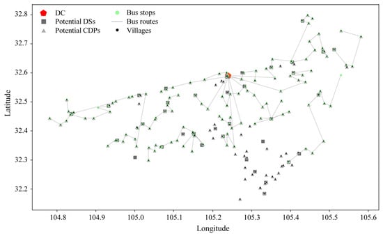
Figure 5.
Distribution of villages, potential CDPs and DSs, the DC, and bus routes and stops.
5.1. Parameter Setting
To ensure that the results are authentic and stable, the values of the parameters used have been taken from the real world and from published literature on network design [17,26,27,28,41,52]. Among these, the parcel delivery and pickup demand for each village is calculated by multiplying the village population by the per capita demand. On average, the per capita daily delivery and pickup demand are 0.05 and 0.01 pieces, respectively. The distance between any two nodes is obtained from Gaode Maps (Version v.13). The values of the other parameters are listed in Table 3.
Table 3.
Parameters used in real-world case.
The parameters for the three-phase ALNS algorithm are set as follows. The initial temperature is . The annealing coefficient is 0.885. The predefined minimum values for tempering and annealing are and , respectively. The tempering temperature and tempering coefficient are and 1.005, respectively. The number of consecutive iterations without improvement is 15. The scores for operators , , and are 15, 12, and 5, respectively. The importance of operator scores is 0.2.
5.2. Performance of the Three-Phase ALNS Algorithm
To demonstrate the performance of the three-stage ALNS algorithm, we compare its results with those of the GUROBI solver and the standard ALNS algorithm. Four test cases are randomly generated from the Qingchuan case scenario, and each algorithm is run 20 times to obtain an average result (as shown in Table 4). For the GUROBI solver, the termination criteria are set to either a gap of 0.001% or a maximum solution time of 10,800 s. , , , and represent the numbers of potential DSs, potential CDPs, villages, and fixed-route buses, respectively. and represent the relaxed lower bound and feasible upper bound target values, respectively. The GAP is calculated as . For the two ALNS algorithms, represents the average of 20 results, while the GAP is obtained by calculating .
Table 4.
Comparison of results generated by the three solution algorithms.
Table 4 shows that the three-phase ALNS algorithm exhibits better solution efficiency and quality. For the small-scale test case (5-21-21-3), the three-phase ALNS algorithm produces a solution that is only 1.32% higher than the optimal solution but takes only 3.38% of the time required by the GUROBI solver. For medium-scale test cases (7-35-35-6 and 8-45-45-7), the three-phase ALNS algorithm can find solutions that are 2.61% lower and 2.32% higher than those of GUROBI in 67 and 140 s, respectively. Its GAP values are also 0.5 and 1.9 percentage points lower than those of the standard ALNS algorithm. For the large-scale test case (22-100-100-13) that cannot be solved by GRROBI, the three-phase ALNS algorithm achieves a solution that is 2.08% lower than that obtained using the standard ALNS algorithm.
5.3. Case Result
We solved the case ten times, achieving an average total network cost of CNY 11,727 and an average solution time of 2485 s. The optimal solution costs CNY 11,462 in total, and the corresponding location–routing proposal is shown in Figure 6. Among these, 17 DSs and 82 CDPs need to be established, utilizing 21 schedules across 18 routes, 15 mini-trucks, and 5 small trucks to provide parcel pickup and delivery services. The travel distances for mini-trucks and small trucks are 1043.57 km and 590.28 km, respectively. The maximum and average self-service distances for customers in villages are 4.98 and 1.71 km, respectively.
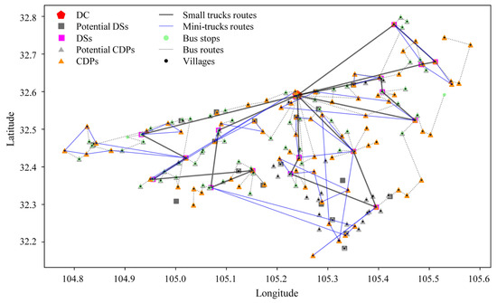
Figure 6.
Benchmark results for the case study.
The effectiveness of the proposed synergistic trucks and fixed-route buses proposal is verified by comparing it with a trucks-only scenario. As shown in Table 5, the synergistic solution offers cost savings, reducing the total network cost by 5.03% compared to the trucks-only scenario. This equates to annual savings of around CNY 220,000. The cost savings mainly come from three areas: the travel distance of micro trucks (reduced by 43.22%), the number of CDPs (reduced by four), and the number of small trucks (reduced by one). However, the fixed bus routes result in indicators such as the average self-service distance, the number of DSs, and the travel distance of small trucks being inferior to those in the trucks-only scenario.
Table 5.
Comparison of synergistic trucks and fixed-route bus scenario and trucks-only scenario.
5.4. Sensitivity Analysis
- (1)
- Parcel transport capacity of bus route
As shown in Figure 7, the total network cost fluctuates as the parcel transport capacity gradually decreases from 300 to 100. The cost is lowest at a capacity of 250. Although small trucks travel longer distances, the 250-capacity network plan performs better in other respects, with five indicators outperforming those of other capacity schemes. When capacity increases to 300, the number of DSs and CDPs increases, as does the use and travel distance of small trucks and the number of bus schedules. Therefore, a higher capacity does not generate greater cost savings. However, lower bus capacities (such as 150 and 100) would require more trucks to transport parcels, thereby increasing the total cost.
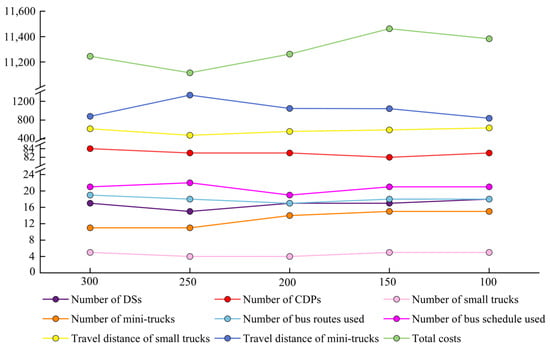
Figure 7.
Influence of parcel transport capacity of bus route on network schemes.
- (2)
- Maximum service radius of CDPs
As shown in Figure 8, the total network cost increases gradually from CNY 11,146 to CNY 14,253 as the maximum service radius decreases from 6 km to 3 km. The main reasons for the increase in costs are the rise in the number of CDPs (from 77 to 123, an increase of around 60%) and the increase in the travel distance of mini-trucks (from 1009.23 km to 1662.40 km, an increase of around 65%). However, reducing the maximum service radius improves the accessibility of delivery logistics services, with the average self-service distance falling from 2.09 km to 0.61 km. In terms of total cost and accessibility, the scheme corresponding to 4 km is clearly more advantageous. Compared with the scheme corresponding to 5 km, the cost increased by only 7.02%, while the average self-pickup distance decreased by 47.37%.
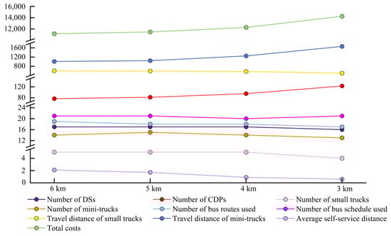
Figure 8.
Influence of the maximum service radius of CDPs on network schemes.
- (3)
- Target service radius of CDPs
As shown in Figure 9, the total network cost increases slightly from CNY 11,295 to CNY 11,707 as the target service radius decreases from 5 to 2 km. There are five indicators that are significantly affected by the target service radius: the numbers of CDPs and small trucks, the travel distances of mini- and small trucks, and the average self-service distance. It is worth noting that the network scheme corresponding to 4 km offers the most obvious comprehensive advantages in terms of cost and service accessibility, which is consistent with the maximum service radius analysis. Compared with the network scheme corresponding to 5 km, it achieved a reduction in the average self-service distance of 11.58% with only a 0.67% increase in cost.
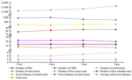
Figure 9.
Influence of the target service radius of CDPs on network schemes.
Overall, sensitivity analysis indicates that variations in all three parameters significantly impact total network costs, but through different mechanisms. There is a nonlinear relationship between total cost and the parcel delivery capacity of bus routes, with the total cost reaching its optimal value when the capacity is 250. Furthermore, upon analyzing the trade-off between cost and service accessibility reflected in the two service radius parameters, it is shown that a 4 km radius achieves the optimal balance between operational expenditure and service accessibility. With that outcome in mind, the following concise recommendations are offered to planning authorities and CSPs. First, the “Goldilocks Principle” should be applied to determine the service radius of self-pickup facilities. Planners should not pursue maximum service coverage or minimum service costs in isolation but rather establish a balanced service radius. As demonstrated by the findings of Sun et al. [17] and this study, a marginal increase in costs often yields a higher proportion of accessibility improvements. Second, buses that accommodate both passenger travel requirements and parcel delivery demands should be designed. Aiming for greater parcel capacities in buses may not translate into lower network costs and could potentially compromise passenger satisfaction. Therefore, as suggested by He et al. [15] and Gharaei et al. [53], vehicle capacity and quantity should be reasonably configured based on specific regional conditions to achieve system-wide efficiency optimization.
6. Conclusions and Further Research Directions
6.1. Conclusions
This study introduces a three-echelon rural delivery logistics network design scheme that synergizes trucks and fixed-route buses. As a new type of FOT, our scheme allows fixed-route buses and trucks to operate in a parallel manner. It is formulated as a 3E-LRP-TF model, and a three-phase algorithm is designed based on the ALNS for model solving. A case study from China demonstrates the practicality of our mathematical model and proposed algorithm. Optimal results demonstrate that the three-phase ALNS algorithm can provide excellent solutions within a reasonable timeframe. It also shows that the synergistic network can achieve cost savings of over 5% compared to a trucks-only network, saving CNY 220,000 per year in the case study area. In addition, sensitivity analysis reveals that the parcel transport capacity of bus routes exhibits a nonlinear effect on total costs, with an optimal cost value observed when set at 250. For two service radius parameters, the trade-off between cost and accessibility is clearly reflected, with 4 km emerging as the balanced compromise.
These main findings also validate the scalability and transferability of the framework. On one hand, the core mechanism of synergy between fixed-route buses and trucks is applicable to any IPFT service scenario with a large number of rural communities. The parameter-driven structure of the model enables high transferability, allowing flexible customization across diverse rural scenarios without structural modifications, thereby providing a practical solution for regional logistics planning in heterogeneous operational contexts. On the other hand, the high-efficiency performance of the three-phase ALNS algorithm enables it to deliver high-quality solution results for current large-scale networks and even for networks that will expand in the future. Additionally, the separable structure of this algorithm enables its application in vehicle route optimization and scheduling for daily operations, providing computational support for operational decision making.
6.2. Further Research Directions
Of course, this study has several limitations, which may lead to practical research in the future. On the one hand, the successful implementation of this hybrid system depends on operational protocols and regulatory requirements that provide a balance between efficient freight movement and excellent passenger service. Therefore, as advocated by Yang et al. [42], passenger comfort and safety should be given greater priority. Another consideration pertains to the green initiative and the public facility nature of CDPs; it is also reasonable to consider pollutant emissions and service equity as additional objectives. On the other hand, it is also possible to consider combining the proposed algorithm with other heuristic or artificial intelligence algorithms to efficiently support real-time decision making [54]. Furthermore, broader case studies can be conducted to effectively explore the impact of real-world factors (e.g., demand fluctuations, varying fuel prices, and bus route changes) and formulate more universally applicable policy recommendations.
Author Contributions
Conceptualization, J.Z., J.L. and W.S.; methodology, J.L. and W.S.; software, J.L.; data curation, J.L. and W.L.; writing—original draft preparation, W.S. and J.Z.; writing—review and editing, W.S. and J.Z.; supervision, J.Z. All authors have read and agreed to the published version of the manuscript.
Funding
This research was funded by the National Natural Science Foundation of China, grant number 72173101.
Data Availability Statement
The data and algorithm code presented in this study are available on request from the corresponding author due to ongoing further research.
Conflicts of Interest
The authors declare no conflicts of interest.
Abbreviations
The following abbreviations are used in this manuscript:
| 3E-LRP-TF | Three-echelon location–routing problem that synergizes trucks and fixed-route buses |
| ALNS | Adaptive large neighborhood search |
| CDP | Pickup and delivery point |
| CSP | Courier, express, and parcel service provider |
| DC | Distribution center |
| DS | Distribution station |
| FOT | Freight on transit |
| SAR | Share-a-ride |
References
- Couture, V.; Faber, B.; Gu, Y.Z.; Liu, L.Z. Connecting the Countryside via E-Commerce: Evidence from China. Am. Econ. Rev. Insights 2021, 3, 35–50. [Google Scholar] [CrossRef]
- Shin, N.; Lim, H.; Kim, Y.J. Modeling spatial dimensions of parcel delivery demand and its determinants. Int. J. Logist-Res. App. 2023, 28, 1002–1018. [Google Scholar] [CrossRef]
- Rai, H.B.; Dablanc, L. Hunting for treasure: A systematic literature review on urban logistics and e-commerce data. Transp. Rev. 2023, 43, 204–233. [Google Scholar] [CrossRef]
- Nikolić, I.; Milutinović, J.; Božanić, D.; Dobrodolac, M. Using an Interval Type-2 Fuzzy AROMAN Decision-Making Method to Improve the Sustainability of the Postal Network in Rural Areas. Mathematics 2023, 11, 3105. [Google Scholar] [CrossRef]
- CIECC. Rural E-Commerce Development Report in China (2021–2022); China International E-commerce Center: Chengdu, China, 2022. [Google Scholar]
- De Meyer, A.; Guisson, R.; Verbelen, G.; Van Hulle, F. The impact of different cooperation strategies on the efficiency of rural parcel deliveries. Transp. Res. Procedia 2023, 72, 2331–2338. [Google Scholar] [CrossRef]
- Sousa, R.; Horta, C.; Ribeiro, R.; Rabinovich, E. How to serve online consumers in rural markets: Evidence-based recommendations. Bus. Horiz. 2020, 63, 351–362. [Google Scholar] [CrossRef]
- RISC. Package Delivery in Rural and Dense Urban Areas; United States Postal Service: Washington, DC, USA, 2020. [Google Scholar]
- Wu, S.; Yang, Q.; Yang, Z. Integrating express package delivery service with offline mobile sales: A new potential solution to sustainable last-mile logistics in rural China. Int. J. Logist. Res. Appl. 2025, 28, 121–149. [Google Scholar] [CrossRef]
- Stead, D. The European green paper on urban mobility. Eur. J. Transp. Infrastruct. Res. 2007, 7, 4. [Google Scholar] [CrossRef]
- Cochrane, K.; Saxe, S.; Roorda, M.J.; Shalaby, A. Moving freight on public transit: Best practices, challenges, and opportunities. Int. J. Sustain. Transp. 2017, 11, 120–132. [Google Scholar] [CrossRef]
- Qu, X.B.; Wang, S.A.; Niemeier, D. On the urban-rural bus transit system with passenger-freight mixed flow. Commun. Transp. Res. 2022, 2, 100054. [Google Scholar] [CrossRef]
- Cavallaro, F.; Nocera, S. Flexible-route integrated passenger-freight transport in rural areas. Transp. Res. A-Pol. 2023, 169, 103604. [Google Scholar] [CrossRef]
- Bruzzone, F.; Cavallaro, F.; Nocera, S. The integration of passenger and freight transport for first-last mile operations. Transp. Policy 2021, 100, 31–48. [Google Scholar] [CrossRef]
- He, D.D.; Ceder, A.; Zhang, W.Y.; Guan, W.; Qi, G.Q. Optimization of a rural bus service integrated with e-commerce deliveries guided by a new sustainable policy in China. Transp. Res. E-Log. 2023, 172, 103069. [Google Scholar] [CrossRef]
- Elbert, R.; Rentschler, J. Freight on urban public transportation: A systematic literature review. Res. Transp. Bus. Manag. 2022, 45, 100679. [Google Scholar] [CrossRef]
- Sun, W.J.; Zhang, J.; Liu, J.; Li, G.Q. Delivery Logistics Network Design for Mountainous Rural Areas with Parcel Transportation by Bus and Simultaneous Home Delivery and Customer Self-pickup. J. Transp. Syst. Eng. Inf. Technol. 2024, 24, 94–102. [Google Scholar] [CrossRef]
- MOT. Guiding Opinions on Accelerating the Integrated Development of Passenger and Freight Transportation Combined Postal Services in Rural Areas. 2023. Available online: https://www.transformcn.com/Regulations/785.html (accessed on 30 December 2024).
- Cheng, R.; Jiang, Y.; Nielsen, O.A. Integrated people-and-goods transportation systems: From a literature review to a general framework for future research. Transp. Rev. 2023, 43, 997–1020. [Google Scholar] [CrossRef]
- Eiselt, H.A.; Gendreau, M.; Laporte, G. Arc routing problems, part II: The rural postman problem. Oper. Res. 1995, 43, 399–414. [Google Scholar] [CrossRef]
- Seghezzi, A.; Mangiaracina, R.; Tumino, A. E-grocery logistics: Exploring the gap between research and practice. Int. J. Logist. Manag. 2023, 34, 1675–1699. [Google Scholar] [CrossRef]
- Feng, Z. Constructing rural e-commerce logistics model based on ant colony algorithm and artificial intelligence method. Soft Comput. 2020, 24, 7937–7946. [Google Scholar] [CrossRef]
- Yang, Z.; Han, H.; Yansui, L. The spatial distribution characteristics and influencing factors of Chinese villages. Acta Geogr. Sin. 2020, 75, 2206–2223. [Google Scholar] [CrossRef]
- Hu, M.; Monahan, S. US E-Commerce Trends and the Impact on Logistics; AT Kearney: Chicago, IL, USA, 2016. [Google Scholar]
- Morganti, E.; Dablanc, L.; Fortin, F. Final deliveries for online shopping: The deployment of pickup point networks in urban and suburban areas. Res. Transp. Bus. Manag. 2014, 11, 23–31. [Google Scholar] [CrossRef]
- Yang, C.; Shu, T.; Liang, S.; Chen, S.; Wang, S. Vehicle routing optimization for rural package collection and delivery integrated with regard to the customer self-pickup radius. Appl. Econ. 2023, 55, 4841–4852. [Google Scholar] [CrossRef]
- Dai, Y.; Luo, J.; Yang, F.; Ma, Z. A Location-routing Problem in Rural Delivery Systems with Service Radius Decisions. Syst. Eng. 2023, 41, 43–52. [Google Scholar]
- Sun, W.; Zhang, J.; Shen, H.; Li, G.; Yang, J.; Hong, Z. Joint optimization of parcel delivery periodic location-routing and prepositioning disaster response facilities. In Proceedings of the 2023 7th International Conference on Transportation Information and Safety (ICTIS), Xi’an, China, 4–6 August 2023; pp. 530–537. [Google Scholar]
- Zhang, R.; Dai, Y.; Yang, F.; Ma, Z. A cooperative vehicle routing problem with delivery options for simultaneous pickup and delivery services in rural areas. Socio-Econ. Plan. Sci. 2024, 93, 101871. [Google Scholar] [CrossRef]
- Xiao, J.; Li, Y.; Cao, Z.; Xiao, J. Cooperative trucks and drones for rural last-mile delivery with steep roads. Comput. Ind. Eng. 2024, 187, 109849. [Google Scholar] [CrossRef]
- Jiang, J.; Dai, Y.; Yang, F.; Ma, Z. A multi-visit flexible-docking vehicle routing problem with drones for simultaneous pickup and delivery services. Eur. J. Oper. Res. 2024, 312, 125–137. [Google Scholar] [CrossRef]
- Yang, F.; Dai, Y.; Ma, Z.-J. A cooperative rich vehicle routing problem in the last-mile logistics industry in rural areas. Transp. Res. Part. E Logist. Transp. Rev. 2020, 141, 102024. [Google Scholar] [CrossRef]
- Cavallaro, F.; Nocera, S. Integration of passenger and freight transport: A concept-centric literature review. Res. Transp. Bus. Manag. 2022, 43, 100718. [Google Scholar] [CrossRef]
- Rzesny-Cieplinska, J. Overview of the practices in the integration of passenger mobility and freight deliveries in urban areas. Case Stud. Transp. Pol. 2023, 14, 101106. [Google Scholar] [CrossRef]
- Derse, O.; Van Woensel, T. Integrated People and Freight Transportation: A Literature Review. Future Transp. 2024, 4, 1142–1160. [Google Scholar] [CrossRef]
- Bruzzone, F.; Cavallaro, F.; Nocera, S. Environmental and energy performance of integrated passenger–freight transport. Transp. Res. Interdiscip. Perspect. 2023, 22, 100958. [Google Scholar] [CrossRef]
- Ringsberg, H. Sustainable FLM transport based on IPF transport by ferry in coastal rural areas: A case from Sweden. Transp. Res. A-Pol. 2023, 178, 03871. [Google Scholar] [CrossRef]
- Li, B.X.; Krushinsky, D.; Reijers, H.A.; Van Woensel, T. The Share-a-Ride Problem: People and parcels sharing taxis. Eur. J. Oper. Res. 2014, 238, 31–40. [Google Scholar] [CrossRef]
- Lu, C.C.; Diabat, A.; Li, Y.T.; Yang, Y.M. Combined passenger and parcel transportation using a mixed fleet of electric and gasoline vehicles. Transp. Res. E-Log. 2022, 157, 102546. [Google Scholar] [CrossRef]
- He, D.D.; Guan, W. Promoting service quality with incentive contracts in rural bus integrated passenger-freight service. Transp. Res. a-Pol. 2023, 175, 103781. [Google Scholar] [CrossRef]
- Feng, W.H.; Tanimoto, K.; Chosokabe, M. Feasibility analysis of freight-passenger integration using taxis in rural areas by a mixed-integer programming model. Socio-Econ. Plan. Sci. 2023, 87, 101539. [Google Scholar] [CrossRef]
- Yang, T.N.; Chu, Z.Z.; Wang, B.L. Feasibility on the integration of passenger and freight transportation in rural areas: A service mode and an optimization model. Socio-Econ. Plan. Sci. 2023, 88, 101665. [Google Scholar] [CrossRef]
- Masson, R.; Trentini, A.; Lehuédé, F.; Malhéné, N.; Péton, O.; Tlahig, H. Optimization of a city logistics transportation system with mixed passengers and goods. EURO J. Transp. Logist. 2017, 6, 81–109. [Google Scholar] [CrossRef]
- Schmidt, J.; Tilk, C.; Irnich, S. Using public transport in a 2-echelon last-mile delivery network. Eur. J. Oper. Res. 2024, 317, 827–840. [Google Scholar] [CrossRef]
- Azcuy, I.; Agatz, N.; Giesen, R. Designing integrated urban delivery systems using public transport. Transp. Res. E-Log. 2021, 156, 102525. [Google Scholar] [CrossRef]
- Wang, L.; Li, Q.; Zhou, X.C.; Yang, L.L. Research on The Routing Problem of Rural Delivery Logistics in Mountainous Areas under The Cooperative Distribution of Bus-Electric Vehicle-Drone. J. Syst. Sci. Math. Sci. 2025, 1–23. [Google Scholar] [CrossRef]
- Delle Donne, D.; Santini, A.; Archetti, C. Integrating public transport in sustainable last-mile delivery: Column generation approaches. Eur. J. Oper. Res. 2025, 324, 75–91. [Google Scholar] [CrossRef]
- Zhang, X.; Wang, Y.; Zhang, D. Location-Routing Optimization for Two-Echelon Cold Chain Logistics of Front Warehouses Based on a Hybrid Ant Colony Algorithm. Mathematics 2024, 12, 1851. [Google Scholar] [CrossRef]
- Hoseini Shekarabi, S.A.; Gharaei, A.; Karimi, M. Modelling and optimal lot-sizing of integrated multi-level multi-wholesaler supply chains under the shortage and limited warehouse space: Generalised outer approximation. Int. J. Syst. Sci. Oper. Logist. 2019, 6, 237–257. [Google Scholar] [CrossRef]
- Contardo, C.; Hemmelmayr, V.; Crainic, T.G. Lower and upper bounds for the two-echelon capacitated location-routing problem. Comput. Oper. Res. 2012, 39, 3185–3199. [Google Scholar] [CrossRef]
- Gandra, V.M.S.; Çalık, H.; Wauters, T.; Toffolo, T.A.M.; Carvalho, M.A.M.; Vanden Berghe, G. The impact of loading restrictions on the two-echelon location routing problem. Comput. Ind. Eng. 2021, 160, 107609. [Google Scholar] [CrossRef]
- Zhou, X.; Zhao, C.; Xie, F. Collaborative Delivery Route Planning for Rural Public Buses and Express Delivery Vehicles Based on Passenger and Freight Integration. Transp. Res. Rec. 2025, 2679, 381–408. [Google Scholar] [CrossRef]
- Gharaei, A.; Karimi, M.; Hoseini Shekarabi, S.A. An integrated multi-product, multi-buyer supply chain under penalty, green, and quality control polices and a vendor managed inventory with consignment stock agreement: The outer approximation with equality relaxation and augmented penalty algorithm. Appl. Math. Model. 2019, 69, 223–254. [Google Scholar] [CrossRef]
- Soto-Concha, R.; Escobar, J.W.; Morillo-Torres, D.; Linfati, R. The Vehicle-Routing Problem with Satellites Utilization: A Systematic Review of the Literature. Mathematics 2025, 13, 1092. [Google Scholar] [CrossRef]
Disclaimer/Publisher’s Note: The statements, opinions and data contained in all publications are solely those of the individual author(s) and contributor(s) and not of MDPI and/or the editor(s). MDPI and/or the editor(s) disclaim responsibility for any injury to people or property resulting from any ideas, methods, instructions or products referred to in the content. |
© 2025 by the authors. Licensee MDPI, Basel, Switzerland. This article is an open access article distributed under the terms and conditions of the Creative Commons Attribution (CC BY) license (https://creativecommons.org/licenses/by/4.0/).