Abstract
This study presents an innovative numerical method for solving linear fractional differential equations (LFDEs) using modified Bernstein polynomial bases. The proposed approach effectively addresses the challenges posed by the nonlocal nature of fractional derivatives, providing a robust framework for handling multiple initial and boundary value constraints. By integrating the LFDEs and approximating the solutions with modified fractional-order Bernstein polynomials, we derive operational matrices to solve the resulting system numerically. The method’s accuracy is validated through several examples, showing excellent agreement between numerical and exact solutions. Comparative analysis with existing data further confirms the reliability of the approach, with absolute errors ranging from 10−18 to 10−4. The results highlight the method’s efficiency and versatility in modeling complex systems governed by fractional dynamics. This work offers a computationally efficient and accurate tool for fractional calculus applications in science and engineering, helping to bridge existing gaps in numerical techniques.
Keywords:
Bernstein polynomials; operational matrices; initial and boundary value problems; fractional differential equations; numerical approximation; Caputo derivative MSC:
12-XX; 32-XX; 41-XX
1. Introduction
This paper introduces a novel numerical method addressing key limitations in existing approaches for solving linear fractional differential equations (LFDEs). Fractional calculus is pivotal for modeling anomalous transport and memory-dependent phenomena in physics, engineering, biology, and finance [1,2,3,4,5]. Linear fractional partial differential equations (LFPDEs) are indispensable for modeling nonlocal and memory-driven phenomena. However, their analytical intractability frequently necessitates robust numerical frameworks [6,7]. The nonlocal nature of fractional derivatives presents specific challenges, such as disrupting the periodicity of periodic functions [8]. This poses a critical challenge for analyzing dynamical systems governed by such operators [9]. The absence of a systematic stability framework for fractional-order delay systems contrasted with mature theories for integer-order systems reflects unresolved challenges posed by memory effects and power-law kernels [10]. By integrating Genocchi polynomials with semi-orthogonal bases, this study develops operational matrices tailored for solving fractional differential equations, bridging gaps in handling nonlinearity and nonlocality [11]. Fractional models better capture nonlocal effects and memory phenomena in complex systems (e.g., fractal geometries, turbulent flow) [1,12]. Unlike integer-order derivatives, fractional derivatives are nonlocal, enabling accurate modeling of irregular or discontinuous dynamics [13,14]. Extending the proposed error estimation method to time fractional PDEs and exploring applications in multi-physics systems [15,16]. The work underscores the need for robust numerical frameworks to handle the singularity and complexity of linear and nonlinear FDEs [17,18,19].
There are various existing methods for solving linear and nonlinear fractional differential equation (FDE) problems [20,21,22,23], but many of these techniques have limitations. Therefore, a new approach is needed. This study introduces a novel procedure for solving linear fractional differential equations using an integral method. While exploring different solution strategies, we identified several drawbacks in existing methods, reinforcing the need for our proposed approach [24,25,26,27,28,29,30].
For the reasons mentioned above, fractional calculus is a key tool for modeling modern complex systems and is also indispensable for capturing nonlocal and memory-driven phenomena in various fields, including physics, engineering, biology, and finance [1,2,3,4,5]. Although several existing methods have been implemented, many of these techniques still possess significant limitations, and most methods are analytical methods. Although several methods exist for solving fractional differential equations (FDEs), such as the Runge–Kutta method, Taylor series expansions, and finite difference methods, they often struggle with complex or nonlinear problems [31]. For instance, techniques that combine Sawi with iterative methods still face limitations inherent to these traditional approaches [31].
Another author uses finite difference schemes and spectral methods to solve FDEs [32]. It has limitations due to Numerical methods for fractional calculus, such as finite difference and spectral schemes, which face significant challenges, including poor error control, high computational costs for multidimensional data, and inefficiency with complex geometries. These difficulties are compounded by the nonlocal nature of fractional operators, which leads to theoretical complexity and practical issues like numerical instability and uncertain convergence. Furthermore, the absence of a standardized methodology for choosing between fractional operators that yield different results remains a significant obstacle in the field [32].
Another study uses the shifted Jacobi method, which employs Jacobi polynomials within a conformable fractional derivative framework to solve second-order singular periodic boundary value problems [33]. The method can be computationally intensive and complex to implement compared to simpler polynomial bases, and may converge slowly, particularly for large systems or matrices with poorly scaled elements [33]. Another study proposes a meshless Generalized Finite Difference Method (GFDM) for discretizing spatial derivatives, which uses moving least squares and a weight function to optimize a weighted Taylor series based on node distance for approximating Caputo and Riemann–Liouville fractional derivatives [34]. The method proves “conditional convergence”, which means its convergence depends on certain conditions [34].
The Tantawy Technique is a fast, computationally efficient method that uses direct compensation for high accuracy [35]. In contrast, the Variational Iteration Transform Method (VITM) employs correction functionals to solve nonlinear differential equations without linearization [35]. The Variational Iteration Transform Method (VITM) requires expertise in variational calculus to identify the Lagrange multiplier effectively [35]. Another study employs a hybrid method combining a finite difference L1 scheme on a graded mesh for temporal discretization of the Caputo derivative and a Generalized Jacobi Petrov–Galerkin spectral approach with non-smooth basis functions for spatial discretization, effectively handling non-smooth solutions [36]. Achieving high-order accuracy in finite difference/spectral methods relies on often unrealistic smoothness assumptions, facing spatial challenges with non-guaranteed smoothness in spectral methods and temporal limitations in handling non-smooth solutions on uniform meshes, as hybrid approaches generally presume smoothness in at least one dimension [36]. Given these persistent challenges and limitations across existing numerical approaches, the development of novel, more versatile numerical techniques remain essential to accurately and efficiently solve fractional differential equations.
To address these challenges and numerical gaps, we outline a new computational technique to solve fractional differential equations. We begin by introducing the classical Bernstein polynomials and subsequently extend them into fractional Bernstein polynomials through the application of Caputo’s fractional derivative. The structure of the method begins by integrating the linear fractional differential equation and applying the initial and boundary conditions as integration limits. We assume an approximate solution as a linear combination of modified fractional B-polys, called Bhatti fractional B-polys. This approximation is then substituted into the integral form of the linear fractional differential equation. The resulting equation is solved using an operational matrix approach, and the unknown coefficients are determined to obtain the final solution. To gauge the accuracy of our method, we apply it to three examples of linear fractional differential equations in this study. We then perform an error analysis to demonstrate the accuracy and efficiency of the proposed method.
This study is structured as follows. First, the Introduction establishes the necessity for a novel numerical technique by discussing the limitations of existing methods in solving fractional differential equations. Next, the Methodology section details the theoretical foundation of the proposed approach, including the construction of fractional Bernstein polynomial bases and operational matrices. The Implementation section describes the application of this method to specific problem types, followed by Numerical Examples, where the method is tested on several benchmark problems. Error Analysis is then performed to evaluate the accuracy and robustness of the solutions. Finally, the Conclusion summarizes the findings, highlights the advantages of the proposed technique, and suggests potential directions for future research.
2. Fractional-Order Bernstein Polynomials Basis
The generalized form of fractional B-polys , expressed in terms of the variable x or t over the interval or , is defined in the referenced sources [26,37],
where represents the fractional order of B-polys. In this equation, is described as,
The coefficient of binomial is expressed as .
3. Caputo’s Fractional Derivative
We compute fractional derivatives using Caputo’s operator. Fractional derivatives are computed via Caputo’s operator [38], formulated as:
where denotes the fractional order, represents the gamma function, and is the nth integer-order derivative of . The Caputo derivative notably facilitates direct incorporation of initial and boundary conditions, making it consistent with physical systems [38]. The Caputo derivative of polynomial is given by
where denotes the fractional order function. The one-dimensional approximate solution is represented as a series expansion in terms of fractional-order B-polys . Specifically, the estimated solution to the linear fractional differential equation is expressed in the form:
where are the expansion coefficients in Equation (5). Let us examine a canonical linear fractional differential equation (FDE) of order , expressed in the form, ref. [30]:
Integrating both sides with respect to the variable , where are constants. Applying the initial and boundary conditions to the equation, we obtain [30,39]:
By substituting the approximate solution , Equation (5) into Equation (7) in above equation. We then separate the coefficient term as vector , and represent the remaining terms as a matrix on the left-hand side, while denoting the right-hand side as column matrix . This leads to the operational matrix equation . This equation is solved numerically to determine the unknown coefficients . Substituting these coefficients back into the approximate solution then yields the approximated numerical solution. We evaluated our method’s accuracy by solving various linear fractional equations and calculating absolute errors.
4. Examples
In this section, we present three illustrative examples to thoroughly evaluate the accuracy and effectiveness of the proposed method. These examples are carefully chosen to represent a diverse set of fractional differential equations involving various initial and boundary conditions. The goal is to demonstrate the method’s robustness and adaptability in handling complex problems across different scenarios. Due to its flexible framework, the method is expected to be highly versatile, capable of addressing both linear and nonlinear cases with high precision. Through these examples, we aim to showcase not only the accuracy of numerical results but also the method’s potential as a reliable tool for solving a wide class of problems in the field of fractional calculus.
Example 1: As a first example, we consider solving a one-dimensional linear fractional differential equation that incorporates both integer-order and non-integer (fractional) derivatives. The equation is given by [40]:
where is given by,
where the terms fractional and represent derivatives of the function with respect to . These fractional derivatives are typically interpreted in the Caputo or Riemann–Liouville sense, depending on the context and required initial/boundary conditions. This equation serves as a benchmark problem to test the accuracy and efficiency of our proposed numerical method. By including derivatives of both integer and low-order fractional degrees, the equation simulates scenarios found in physical systems with memory or hereditary properties, such as anomalous diffusion, porous media flow, or viscoelastic materials. This example illustrates the method’s robustness in handling mixed-order differential operators and its capability to produce highly accurate results even when fractional orders are very small and close to zero.
Employing the initial conditions , , we numerically solve the equation over the interval . The exact solution to Equation (8) is given by
We perform double integration of the equation on both sides as follows:
Twice integration () of both terms with respect to , subject to the given initial condition, produces [30,39]
A simplified representation of this equation is obtained as
The solution to Equation (8) can be approximated using a fractional B-polynomial expansion in the variable:
where represents the unknown expansion coefficient. Substituting these fractional B-polys into Equation (13) and and applying the Galerkin minimization procedure yields [38]
where , , , denote the corresponding matrix operators with elements,
This equation can be expressed in matrix form as
This formulation yields an by system of equations , which is solved numerically for the unknown coefficients as column matrix; these coefficients are then substituted into Equation (14) to obtain the complete solution. Matrices and in Equations (15) and (17) are constructed from inner products of fractional B-polys, computed numerically. The coefficient vector C is determined by solving the linear system derived from Equation (17). The final numerical solution to the fractional differential equation is given by
The numerical solution demonstrates excellent agreement with the exact solution . For this computation, the fractional B-polynomials in Equation (1) were employed in the variables to solve the linear fractional differential Equation (8). As shown in Figure 1, the numerical and exact solutions coincide within machine precision, confirming the high accuracy of the method.
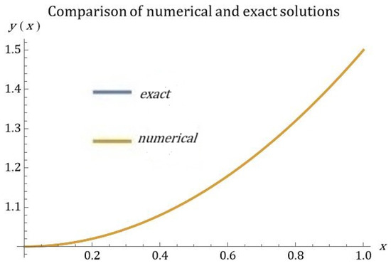
Figure 1.
The approximate solution, , and the exact solutions are depicted in Figure 1. This visual simulation highlights the significant overlap between the two solutions.
Example 2: We now consider solving a third one-dimensional linear fractional differential equation of the form:
where is given by
where represents the classical second-order derivative, and denotes the fractional derivative of order 3/4 = 0.75, which can be interpreted using either the Caputo or Riemann–Liouville definition depending on the initial and boundary conditions.
This equation is particularly interesting because it combines local (integer-order) and nonlocal (fractional-order) differential operators, modeling systems where both instantaneous and memory-dependent behaviors are present. The fractional term introduces a nonlocal influence, capturing effects such as historical dependence or anomalous transport, which are common in complex physical and engineering systems.
The main objective here is to assess how well our numerical method handles the interaction between different derivative orders, especially when fractional orders are less than one, as is the case here. This type of mixed-order equation is more challenging to solve due to the presence of the fractional term, which requires careful numerical treatment.
By applying our proposed method to this problem, we aim to demonstrate its robustness, flexibility, and accuracy in solving fractional differential equations of mixed order across the domain under appropriate boundary conditions and . This example serves as a further test of the proposed numerical method’s effectiveness in handling equations involving both integer- and non-integer-order derivatives, particularly when initial-value conditions are prescribed. The inclusion of a fractional derivative of order 3/4 = 0.75 poses additional challenges due to the nonlocal nature of fractional operators, which depend on the entire history of the solution up to a given point.
We utilize the initial conditions , , and the numerical solution of this equation is sought out in intervals . The exact solution which satisfies initial conditions and Equation (19) is given by
Let us twice integrate the equation on both sides as given below:
The integration twice (I2) of both terms with respect to variable is provided with two initial conditions implemented [30,39],
After first integration of the first term in Equation (22),
After second integration and implementing the initial conditions,
A simplified representation of this equation is obtained:
We approximate that the solution of Equation (19) can be expressed in terms of the fractional B-polys expansion in variable :
where are the unknown expansion coefficients in Equation (23). After substituting these fractional B-polys into Equation (22) using the Galerkin method for minimization [38], we obtain the following expression,
where matrices , , , are represented by matrix elements
We can arrange this equation in terms of matrices so that
This formulation results in an by linear system , which is solved numerically for the expansion coefficients in Equation (34). These coefficients are then substituted into Equation (22) to construct the approximate solution. Matrices and in Equations (24) and (25) are defined through inner products of fractional B-polys, computed numerically. The coefficient vector is determined by solving the linear system derived from Equation (26). The final numerical solution is given by
The above result is highly accurate and matches the exact solution . The B-polys with have been employed in variables in order to solve the linear fractional Equation (26). The perfect agreement between the two results, exact and numerical solutions, at the level of machine accuracy is demonstrated in Figure 2. This solution precisely matches the exact solution, illustrating the effectiveness of the current approach. For this example, we also present a graph to compare the exact solution of the example. The comparative plot visually validates this exact correspondence, demonstrating the approach’s effectiveness.
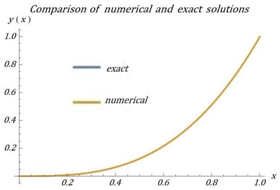
Figure 2.
The approximate solution, , and the exact solutions are depicted in Figure 2. This visual simulation highlights the significant overlap between the two solutions.
Example 3: We now consider a second example involving the solution of a one-dimensional linear fractional differential equation of the form [40]:
where denotes the fractional derivative of order 1.5 with respect to x, typically interpreted in the Caputo or Riemann–Liouville sense. This equation is representative of systems exhibiting super-diffusive behavior, where the dynamics are governed by nonlocal and memory-dependent effects. The inclusion of a non-integer derivative of order greater than one introduces both fractional integration and differentiation into the model, reflecting more complex physical phenomena than traditional integer-order models can capture. This example is used to further validate the proposed numerical method’s ability to handle fractional orders beyond the first derivative and to demonstrate its effectiveness in providing accurate solutions for equations involving higher-order fractional operators.
The function on the right-hand side of Equation (30) is given by
Subject to the boundary conditions, , we seek a numerical solution to this fractional differential equation over the interval . These conditions ensure a well-posed boundary value problem and allow for a meaningful comparison between the numerical and exact solutions. The purpose of this example is to assess the accuracy of the proposed method when applied to a fractional differential equation involving a non-integer derivative of order 1.5. The exact analytical solution of Equation (30) is given by:
which satisfies the boundary conditions and serves as a benchmark for evaluating the performance of the numerical approach. Applying double integration with respect to to both sides of Equation (30), yields an equivalent integral form that can be more suitable for certain numerical methods. Specifically, integrating both sides twice reduces the fractional derivative order and helps in transforming the problem into a form that is more amenable to approximation techniques. Both terms are integrated with respect to while incorporating two initial conditions, yielding the resulting expression is:
This transformation can facilitate the construction of numerical schemes by replacing fractional derivatives with their corresponding integral representations, allowing the use of standard quadrature or interpolation-based methods.
The approximate solution to Equation (30) takes the form of a fractional-order Bernstein polynomial expansion in the spatial variable :
where denotes the expansion coefficient. Substituting the fractional B-polynomial expansion into Equation (33) and applying the Galerkin minimization procedure to Equation (33) yields [38]
This equation can be expressed in matrix form as
where matrices , , and are represented by matrix elements.
Let
The formulation reduces to an by linear system , which is solved numerically for the coefficient of vector . These coefficients are then substituted into Equation (33) to construct the complete solution. The matrices and in Equations (36) and (37) are defined through inner products of fractional B-polynomials, computed numerically. The coefficients are obtained by solving the linear system derived from Equation (36). The final numerical solution is given by
The numerical solution exhibits excellent agreement with the exact solution . Using fractional B-polynomials in variables, we solved the linear fractional Equation (30). Figure 3 and Figure 4 show perfect convergence between the numerical and exact solutions at machine precision level, confirming the method’s accuracy. The exact correspondence between both solutions validates the effectiveness of our approach. For clarity, we include a comparative visualization of the exact and numerical solutions.
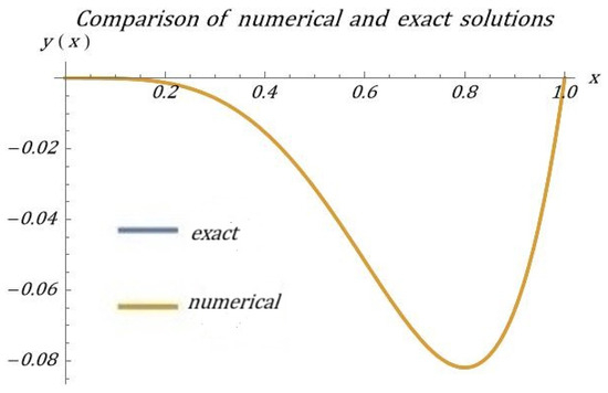
Figure 3.
The approximate solution, , and the exact solutions are depicted in Figure 2. This visual simulation highlights the significant overlap between the two solutions.
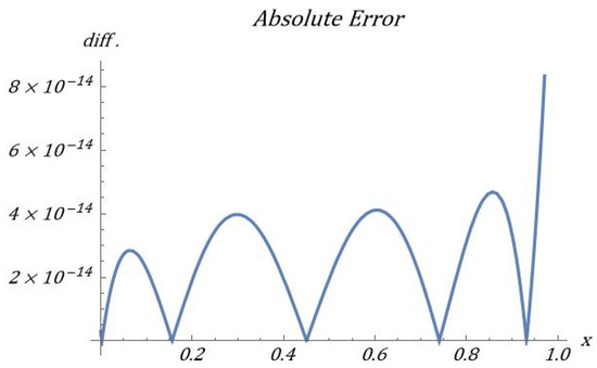
Figure 4.
The picture above presents the absolute error between the exact and approximate solutions for example 3. Notably, the absolute error is on the order of , indicating an extremely high degree of accuracy in the approximation. This level of precision suggests that the approximate solution closely aligns with the exact solution, making it a reliable choice for further analysis or applications.
5. Error Analysis
In this section, we perform an error analysis of examples considered in this study. Table 1 presents a comparison between the exact and the approximate solutions for Example 1 at various values of within the interval . The approximate results were obtained using the proposed numerical method, and the absolute error was calculated as the absolute difference between the exact and numerical solutions divided by a hundred. As shown in Table 1, the error is exceptionally small at the lower end of the interval at and increases gradually with larger values of . The maximum absolute error remains below at , indicating a high level of accuracy across the domain. When compared to the results reported in [40], our method demonstrates significantly improved precision, particularly in the early and mid-range values of . These results validate the effectiveness and reliability of the proposed approach in solving linear fractional differential equations.

Table 1.
For Example, 1, at different values of x, we compare our calculated solution with those from another study [40]. The exact solution is .
Table 2 presents a comparison between the exact and approximate solutions for Example 2 at various values of within the interval [0, 1]. The approximate values were obtained using the proposed numerical method, and the absolute error was calculated as the absolute difference between the exact and approximate solutions divided by a hundred. As shown in the table, the error is exceptionally small at all values of , indicating a high level of accuracy across the domain. These results validate the effectiveness and reliability of the proposed approach in solving linear fractional differential equations.
Table 2.
For Example 2, at different values of , we compare our calculated solution with those from another study [40]. The exact solution is .
Table 3 below presents a comparison between the exact and approximate solutions for Example 3 at various values of x within the interval . The approximate values were obtained using the proposed numerical method, and the absolute error was calculated as the absolute difference between the exact and approximate solutions divided by 100. As shown in the table, the error is exceptionally small at the lower end of the interval at and increases gradually with larger values of x. The maximum absolute error remains below at , indicating a high level of accuracy across the domain. When compared to the results reported in [40], our method demonstrates significantly improved precision at values of x. These results validate the effectiveness and reliability of the proposed approach in solving linear fractional differential equations.
Table 3.
For Example, 3, at different values of x, we compare our calculated solution with those from another study [40]. The exact solution is .
To quantitatively assess the performance of our technique, we compare its results against those of a previously established method [40]. As detailed in Table 1, Table 2 and Table 3, the numerical approximations generated by our method for different problems are in significantly closer agreement with the benchmark solutions than the values reported in [40]. This comparative analysis clearly indicates the enhanced precision and reliability of our proposed approach.
Table 4 demonstrates the convergence properties of the proposed method for Example 3, where the exact solution is given by [40]. The table lists the absolute error at various points for an increasing number of fractional B-polynomial basis functions . The results clearly show that the accuracy of the approximation improves significantly as the size of the basis set is increased, albeit with a corresponding increase in computational cost, as indicated by the CPU time provided in the last row of Table 4. The absolute error approaches zero for the basis set and as shown in the last two columns of Table 4.
Table 4.
For various values of x, we evaluate the absolute error between the approximate solution and the exact solution , considering different numbers of basis functions and corresponding CPU times.
Table 5 shows that the absolute error in Example 1 depends on the fractional order α of the basis set. Although the exact solution in this case is of integer order, the method’s inherent tunability offers a promising direction for future research into problems governed by fractional-order dynamics. It is evident that for α = 0.9 and 0.75, the absolute error is significantly higher, indicating that a greater number of fractional basis functions are required to improve the accuracy of the solution. At the same time, the computational cost increases significantly. Therefore, in these cases, α = 1 was selected for comparison with the exact solutions.
Table 5.
In example 1 the exact solution to the fractional differential equation is . The method’s sensitivity to fractional order values near and is illustrated using absolute error presented in each column. The number of fractional B-polynomials was fixed at , while the fractional order was varied between 0 and 1.
6. Conclusions
Our current methodology effectively solves linear fractional differential equations, extending its previous application to linear and nonlinear ordinary differential equations. This study specifically addresses higher-order fractional differential equations subject to multiple initial and boundary conditions. The method offers high accuracy, with solutions for most fractional equations aligning exactly with known analytical solutions. For the remaining cases, absolute errors, defined as the difference between exact and numerical solutions, are typically on the order of (see Figure 4 and example 3). Solution accuracy is directly influenced by the size of the fractional B-poly basis set employed. Larger basis sets yield more accurate solutions but necessitate more iterations to achieve coefficient convergence, consequently increasing computational time and cost. A notable advantage of our approach is its relative simplicity and accessibility. It avoids grid representation by utilizing a fractional B-polys basis set (Equations (1)–(5)), which reduces the number of iterations needed for coefficient convergence compared to some alternative numerical approaches. This straightforward implementation was realized using the symbolic programming language Mathematica [41].
This study presented an innovative numerical technique for solving linear fractional differential equations (LFDEs) using modified fractional B-polys. The proposed method demonstrated high accuracy and efficiency in handling fractional-order derivatives, as evidenced by the close agreement between numerical and exact solutions across multiple examples. Comparison analyses of all results are provided in four tables in Section 5. Key findings include the following.
The method achieved solutions with absolute errors on the order of , shown in example 3 in Figure 4, showcasing its capability to approximate fractional differential equations with excellent precision. The graphical comparisons further validated the method’s effectiveness, with near-perfect overlaps between exact and numerical solutions. By leveraging fractional B-poly bases and operational matrices, the approach simplified the integration and differentiation processes inherent in fractional calculus. This framework reduced computational complexity while maintaining robustness, even for higher-order fractional derivatives. The computational time for all examples considered here was less than 1–2 min of CPU time. More details on CPU time with respect to the basis set are provided in Table 4.
The technique successfully addresses various LFDEs, including those with multiple initial and boundary conditions, demonstrating its adaptability to diverse problems. The examples spanned different fractional orders and functional forms, underscoring the method’s broad applicability. The study bridged gaps in existing numerical methods by offering a systematic approach to handle nonlocality and memory effects in fractional models. This advancement has potential applications in physics, engineering, and other fields where fractional calculus is pivotal. While the method excels in accuracy, larger basis sets may increase computational costs. Future research could explore optimizations for computational efficiency, extensions to nonlinear fractional equations, and applications in multi-physics systems.
In summary, this work contributes a reliable and accessible numerical framework for solving LFDEs, combining theoretical rigor with practical utility. The results affirm the potential of B-poly bases in fractional calculus, paving the way for further innovations in computational mathematics.
Author Contributions
Conceptualization: M.I.B., Software: M.I.B. Methodology: M.I.B. and N.D., Formal Analysis: M.I.B., N.D. and M.H.R., Validation: M.I.B., N.D. and M.H.R., Data Curation: M.I.B., N.D. and M.H.R., Resources: M.I.B., Project Administration: M.I.B., Investigation: M.I.B., N.D. and M.H.R., Supervision: M.I.B., Writing—Original Draft: M.I.B. and M.H.R., Writing—Review and Editing: M.I.B., N.D. and M.H.R. All authors have read and agreed to the published version of the manuscript.
Funding
This research received no external funding.
Data Availability Statement
The data supporting the findings of this study are available within the article.
Acknowledgments
The authors gratefully acknowledge the use of departmental computing resources for this study.
Conflicts of Interest
The authors declare no competing financial or personal interests that could influence this work.
References
- Sun, H.G.; Zhang, Y.; Baleanu, D.; Chen, W.; Chen, Y.Q. A new collection of real world applications of fractional calculus in science and engineering. Commun. Nonlinear Sci. Numer. Simul. 2018, 64, 213–231. [Google Scholar] [CrossRef]
- Iqbal, M.A.B.; Raza, M.Z.; Khan, A.; Abdeljawad, T.; Almutairi, D.K. Advanced wave dynamics in the STF-mBBM equation using fractional calculus. Sci. Rep. 2025, 15, 1–24. [Google Scholar] [CrossRef]
- Birs, I.; Muresan, C. Fractional-Order Event-Based Control Meets Biomedical Applications. In Computational and Mathematical Models in Biology; Springer: Cham, Switzerland, 2023; pp. 281–304. [Google Scholar] [CrossRef]
- Tien, D.N. Fractional stochastic differential equations with applications to finance. J. Math. Anal. Appl. 2013, 397, 334–348. [Google Scholar] [CrossRef]
- Najafi, A.; Taleghani, R. Fractional Liu uncertain differential equation and its application to finance. Chaos Solitons Fractals 2022, 165, 112875. [Google Scholar] [CrossRef]
- Al-Refai, M.; Baleanu, D.; Al-Refai, M.; Baleanu, D. Comparison principles of fractional differential equations with non-local derivative and their applications. AIMS Math. 2021, 6, 1443–1451. [Google Scholar] [CrossRef]
- Derakhshan, M.H.; Ordokhani, Y. Numerical and stability analysis of linear B-spline and local radial basis functions for solving two-dimensional distributed-order time-fractional telegraph models. J. Appl. Math. Comput. 2025, 71, 2859–2887. [Google Scholar] [CrossRef]
- Tavazoei, M.S. A note on fractional-order derivatives of periodic functions. Automatica 2010, 46, 945–948. [Google Scholar] [CrossRef]
- Singh, M.; Singh, M.P.; Tamsir, M.; Asif, M. Analysis of Fractional-Order Nonlinear Dynamical Systems by Using Different Techniques. Int. J. Appl. Comput. Math. 2025, 11, 47. [Google Scholar] [CrossRef]
- Du, F.; Lu, J.G. New criterion for finite-time stability of fractional delay systems. Appl. Math. Lett. 2020, 104, 106248. [Google Scholar] [CrossRef]
- Baishya, C.; Veeresha, P. Laguerre polynomial-based operational matrix of integration for solving fractional differential equations with non-singular kernel. Proc. R. Soc. A 2021, 477, 86–90. [Google Scholar] [CrossRef]
- Luchko, Y.F.; Rivero, M.; Trujillo, J.J.; Velasco, M.P. Fractional models, non-locality, and complex systems. Comput. Math. Appl. 2010, 59, 1048–1056. [Google Scholar] [CrossRef]
- Abu-Ghuwaleh, M.; Saadeh, R. New definitions of fractional derivatives and integrals for complex analytic functions. Arab. J. Basic. Appl. Sci. 2023, 30, 675–690. [Google Scholar] [CrossRef]
- de Oliveira, E.C. Fractional Derivatives. Stud. Syst. Decis. Control 2019, 240, 169–222. [Google Scholar] [CrossRef]
- Kopteva, N. Pointwise-in-time a posteriori error control for time-fractional parabolic equations. Appl. Math. Lett. 2022, 123, 107515. [Google Scholar] [CrossRef]
- Mohammad, M.; Trounev, A. Computational precision in time fractional PDEs: Euler wavelets and novel numerical techniques. Partial. Differ. Equ. Appl. Math. 2024, 12, 100918. [Google Scholar] [CrossRef]
- Zhang, D.; Wang, Y.; Jiang, K.; Liang, L. Safe optimal robust control of nonlinear systems with asymmetric input constraints using reinforcement learning. Appl. Intell. 2024, 54, 1–13. [Google Scholar] [CrossRef]
- Liu, P.; Meeker, W.Q. Robust Numerical Methods for Nonlinear Regression. 2024. Available online: https://arxiv.org/abs/2403.12759v1 (accessed on 9 April 2025).
- Zhang, S.; Jia, R.; He, D.; Chu, F.; Mao, Z. A general data-driven nonlinear robust optimization framework based on statistic limit and principal component analysis. Comput. Chem. Eng. 2022, 160, 107707. [Google Scholar] [CrossRef]
- Momani, S.; Odibat, Z. Numerical comparison of methods for solving linear differential equations of fractional order. Chaos Solitons Fractals 2007, 31, 1248–1255. [Google Scholar] [CrossRef]
- Rodríguez-Rozas, Á.; Acebrón, J.A.; Spigler, R. The PDD Method for Solving Linear, Nonlinear, and Fractional PDEs Problems. In Nonlocal and Fractional Operators; Springer: Cham, Switzerland, 2021; Volume 26, pp. 239–273. [Google Scholar] [CrossRef]
- AlAhmad, R.; Al-Khaleel, M.; Almefleh, H. On solutions of linear and nonlinear fractional differential equations with application to fractional order RC type circuits. J. Comput. Appl. Math. 2024, 438, 115507. [Google Scholar] [CrossRef]
- Ali, H.M.; Ameen, I.G. Application of various methods to solve some fractional differential equations in different fields. In Fractional Differential Equations; Elsevier: Amsterdam, The Netherlands, 2024. [Google Scholar] [CrossRef]
- Bhatti, M.; Bracken, P.; Dimakis, N.; Herrera, A. Solution of mathematical model for gas solubility using fractional-order Bhatti polynomials. J. Phys. Commun. 2018, 2, 085013. [Google Scholar] [CrossRef]
- Bhatti, M.I.; Bhatta, D.D. Numerical solutions of Burgers’ equation in a B-polynomial basis. Phys. Scr. 2006, 73, 539. [Google Scholar] [CrossRef]
- Bhatti, M.I.; Bracken, P. Solutions of differential equations in a Bernstein polynomial basis. J. Comput. Appl. Math. 2007, 205, 272–280. [Google Scholar] [CrossRef]
- Bhatti, M.I.; Hinojosa, E. 26 results of hyperbolic partial differential equations in B-poly basis. J. Phys. Commun. 2020, 4, 095010. [Google Scholar] [CrossRef]
- Bhatti, M.I.; Rahman, M.H. Technique to Solve Linear Fractional Differential Equations Using B-Polynomials Bases. Fractal Fract. 2021, 5, 208. [Google Scholar] [CrossRef]
- Rahman, M.H.; Bhatti, M.I.; Dimakis, N. Employing a Fractional Basis Set to Solve Nonlinear Multidimensional Fractional Differential Equations. Mathematics 2023, 11, 4604. [Google Scholar] [CrossRef]
- Bhatti, M.I.; Rahman, M.H. A B-Polynomial Approach to Approximate Solutions of PDEs with Multiple Initial Conditions. Axioms 2024, 13, 833. [Google Scholar] [CrossRef]
- Saadeh, R.; Al-Wadi, A.; Qazza, A. Advancing Solutions for Fractional Differential Equations: Integrating the Sawi Transform with Iterative Methods. Eur. J. Pure Appl. Math. 2025, 18, 5583. [Google Scholar] [CrossRef]
- Hafez, M.; Alshowaikh, F.; Voon, B.W.N.; Alkhazaleh, S.; Al-Faiz, H. Review on Recent Advances in Fractional Differentiation and its Applications. Prog. Fract. Differ. Appl. 2025, 11, 245–261. [Google Scholar] [CrossRef]
- Al-Nana, A.; Batiha, I.M.; Jebril, I.H.; Al Khazaleh, S.; Abdeljawad, T. Numerical Solution of Conformable Fractional Periodic Boundary Value Problems by Shifted Jacobi Method. Int. J. Math. Eng. Manag. Sci. 2024, 10, 189–206. [Google Scholar] [CrossRef]
- García, A.; Negreanu, M.; Ureña, F.; Vargas, A.M. On the numerical solution to space fractional differential equations using meshless finite differences. J. Comput. Appl. Math. 2025, 457, 116322. [Google Scholar] [CrossRef]
- El-Tantawy, S.A.; Al-Johani, A.S.; Almuqrin, A.H.; Khan, A.; El-Sherif, L.S. Novel approximations to the fourth-order fractional Cahn–Hillard equations: Application to the Tantawy Technique and other two techniques with Yang transform. J. Low. Freq. Noise Vib. Act. Control 2025, 44, 14613484251322240. [Google Scholar] [CrossRef]
- Chao, Z.; Wang, X.-S.; Zaky, M.A. Finite Difference/Fractional Pertrov–Galerkin Spectral Method for Linear Time-Space Fractional Reaction–Diffusion Equation. Mathematics 2025, 13, 1864. [Google Scholar] [CrossRef]
- Bhatti, M.I. Solutions of the harmonic oscillator equation in a B-polynomial basis. Adv. Stud. Theor. Phys. 2009, 3, 451–460. [Google Scholar]
- Podlubny, I. Fractional Differential Equations: An Introduction to Fractional Derivatives, Fractional Differential Equations, to Methods of Their Solution and Some of Their Applications; Mathematics in Science and Engineering; Academic Press: Cambridge, MA, USA, 1999; Volume 198. [Google Scholar]
- Al-Mazmumy, M.; Alsulami, M. Utilization of the Modified Adomian Decomposition Method on the Bagley-Torvik Equation Amidst Dirichlet Boundary Conditions. Eur. J. Pure Appl. Math. 2024, 17, 546–568. [Google Scholar] [CrossRef]
- Kawala, A.M. Numerical Solution for Initial and Boundary Value Problems of Fractional Order. Adv. Pure Math. 2018, 8, 831. [Google Scholar] [CrossRef]
- Wolfram Research, Inc. Mathematica 14.1, Version 14.1; Wolfram Research, Inc.: Champaign, IL, USA, 2024.
Disclaimer/Publisher’s Note: The statements, opinions and data contained in all publications are solely those of the individual author(s) and contributor(s) and not of MDPI and/or the editor(s). MDPI and/or the editor(s) disclaim responsibility for any injury to people or property resulting from any ideas, methods, instructions or products referred to in the content. |
© 2025 by the authors. Licensee MDPI, Basel, Switzerland. This article is an open access article distributed under the terms and conditions of the Creative Commons Attribution (CC BY) license (https://creativecommons.org/licenses/by/4.0/).