Article

Computing Probabilities of Finding Extremes in a Random Set

by
Gheorghiţă Zbăganu
1,
Anişoara Maria Răducan
1,2 and
Marius Rădulescu
1,*
1
Institute of Mathematical Statistics and Applied Mathematics, “Gh. Mihoc-C. Iacob” Romanian Academy, 050711 Bucharest, Romania
2
Department of Applied Mathematics, Faculty of Cybernetics, Statistics and Economic Informatics, University of Economic Studies of Bucharest, Calea Dorobanti, No. 15-17, Sector 1, 010552 Bucharest, Romania
*
Author to whom correspondence should be addressed.
Mathematics 2025, 13(19), 3074; https://doi.org/10.3390/math13193074
Submission received: 23 July 2025 / Revised: 11 September 2025 / Accepted: 17 September 2025 / Published: 24 September 2025
(This article belongs to the Special Issue Advances in Convex Analysis and Inequalities)

Abstract

This study examines the occurrence of extreme points in random samples of size n obtained by mapping uniformly distributed random variables through a function into a multidimensional space. We focus on the probabilities that such sets contain a unique componentwise maximum, minimum, or both. Our interest lies in the asymptotic behavior of these probabilities. We found that in some cases, for certain irregular mappings, the limits of these probabilities may fail to exist as n tends to infinity. This contrasts with our earlier work, where the assumptions of smoothness and regularity of the mapping function ensured well-behaved limits. In the present study, we investigate scenarios in which these smoothness conditions are relaxed or absent. Because the general multidimensional case is highly challenging, we restrict attention to a simpler but illustrative setting: finite random sets in the plane that lie on the graph of a real function defined over the unit interval. We present partial results in this setting and discuss open questions that remain for future research.

1. Introduction

The subject of the present paper lies within the framework of Random Geometry, which is a field concerned with the probabilistic and geometric properties of random structures. A significant body of work in this area has examined the distribution and number of maximal elements in random subsets of R d , typically of the form S n = { Z 1 , Z 2 , , Z n } , where Z i are random vectors. Early foundational contributions to this topic were made by Barndorff-Nielsen and Sobel, who investigated the geometric boundaries of randomly sampled points in R d (see for instance [1]). Subsequent research has predominantly focused on the number of Pareto maxima—points that are maximal with respect to componentwise partial orderings (see [2,3,4]). Moreover, these studied only trivial cases of our problem, namely, the components of the random vectors are independent and continuous random variables. Even in this case, the research of the abovementioned papers failed to find the distribution of the maximal random vectors and of their number. Only in the case when d = 2 was the distribution found.
We are concerned with the probability that the number of maximal Pareto points is equal to 1. Our work investigates a more specialized scenario: the existence of a true maximum and a true minimum within such random sets—referred to, respectively, as the leader and the antileader. That is, we consider cases where a single point dominates (or is dominated by) all others componentwise, which is a situation that is rarer and more constrained than the general Pareto maximality.
This problem has potential applications across a variety of domains, including mathematical programming, algorithm analysis, multi-criteria decision making, economics, medicine, social sciences, psychology, media, and agriculture. Despite its practical relevance, we found no previous work in the literature that addressed this exact formulation. As a result, we began by developing the foundational tools from scratch.
In a previous study, we developed the computational framework for evaluating these probabilities in discrete, continuous, and absolutely continuous settings (see, for instance, [5]). Furthermore, in [6], we identified conditions under which the sequences ( a n ) , ( b n ) , and ( c n ) —corresponding to the probabilities of observing a maximum, a minimum, and both simultaneously—are convergent.
In this paper, we wanted to see what would happen if f is not a smooth function, as we considered in [5]. Moreover, for simplicity, we analyze only the particular case d = 2 .
We are interested in the following problems:
1. Is it true that the sequences  a n n , b n n , c n n  are always convergent? We will show that it is not true.
2. Is it true that if a n n and b n n are convergent, then c n n is convergent too?
3. If they are convergent, is it true or not that c = a b , where a = l i m a n , b = l i m b n , c = l i m c n ?
We were not able to prove or disprove the questions 2 and 3.
4. How can the function f be characterized as having the property that the sequences a n , b n , c n  are convergent?
We do not yet know all the answers; we summarize the current state of knowledge.
In order to approach it, we consider the simplest case of "bad" function, more exactly, f : [ 0 , 1 ] R 2 , f x = x , 1 A x where 1 A is the indicator function of a Borel set A, i.e., 1 A x = 1 i f x A 0 i f x A .
The existence of the limits a , b depends on the set A. All situations may occur: both a and b exist, only a exists but b does not, a does not exist and b does, or none of them exist.
During our study, we arrived at two very natural problems which perhaps were solved by other authors, but we were not able to find anything about them in the literature. One of them is related to the weak convergence of probabilities: if μ n are probability distributions on the real line and μ n has a weak limit μ , for what Borel sets A is the sequence μ n A n convergent? We present two examples of sets A for which l i m n μ n A does exist and two examples of sets A for which l i m n μ n A does not exist. We show that the problem of finding examples of sets A for which the limit l i m n μ n A does or does not exist is equivalent in the case when A is a countable union of disjoint intervals with the convergence or divergence of some series. More precisely, let α k k and β k k be increasing sequences tending to 1 such that 0 α k β k α k + 1 1 , k 1 . In this case, A = k = 1 α k , β k . Define σ n = k = 1 β k n α k n , n 1 . When does the sequence σ n n have a limit? We were able to find examples of α k k and β k k for which σ n n is convergent and other examples for which it is not. Even if we have a simple criterion to decide if the limit does exist (see Proposition 1), we have no criterion to decide when it does not exist.
The content of the article is organized as follows: Section 2 contains definitions and notation, Section 3 introduces the context of our work, and Section 4 and Section 5 present cases when a , b does or does not exist. The simple proofs are inside the sections, while the more evolved ones are presented in Appendix A.

2. Preliminaries

2.1. Definition and Notation

Let f = f 1 , f 2 : [ 0 , 1 ] R 2 be a measurable arbitrary function, and let the random variable Z = f U , where U U 0 , 1 is uniformly distributed on [ 0 , 1 ] .
Let the functions F Z , F Z : R 2 [ 0 , 1 ] and Φ : R 4 [ 0 , 1 ] be defined as
F Z s , t = P f 1 U s , f 2 U t F Z s , t = P f 1 U s , f 2 U t Φ s 1 , s 2 , t 1 , t 2 = P s 1 f 1 U t 1 , s 2 f 2 U t 2
Note that F Z is the joint distribution function of Z, F Z is the tail of Z, and Φ s 1 , s 2 , t 1 , t 2 represents the probability that Z lies in the rectangle s 1 , t 1 x s 2 , t 2 .
If g : 0 , 1 R is a function and x , y [ 0 , 1 ] are arbitrary, let L y g = λ t : g t g y and H x g = λ t : g t g x where λ : B R R is the Lebesgue measure on R .
Notation. For any f = f 1 , f 2 : 0 , 1 R 2 , we define
ϕ f y = F Z f y = P f 1 U f 1 y , f 2 U f 2 y = λ L y f 1 L y f 2
ψ f x = F Z f x = P f 1 U f 1 x , f 2 U f 2 x = λ H x f 1 H x f 2
η f x , y = Φ Z f x , f y = P f 1 x f 1 U f 1 y , f 2 x f 2 U f 2 y =
= λ L y f 1 L y f 2 H x f 1 H x f 2
Remark 1. 
It is obvious that if h x , y = h 1 x , h 2 y has the property that h 1 and h 2 are increasing, then ϕ h f = ϕ f , ψ h f = ψ f , η h f = η f .

2.2. Simple Facts and Known Results

In [6] was proved that
a n = n F Z n 1 d F Z = 0 1 n F Z n 1 f y d y
b n = n F Z n 1 d F Z = 0 1 n F Z n 1 f x d x
c n = 0 1 0 1 n n 1 Φ Z f x , f y n 2 d y d x
Then, the equalities (2)–(4) become
a n = 0 1 n ϕ f n 1 y d y
b n = 0 1 n ψ f n 1 x d x
c n = 0 1 0 1 n n 1 η f n 2 x , y d y d x
Let a = lim a n , b = lim b n , and c = lim c n , provided that these sequences are convergent.
We shall be interested in the particular case f x = x , 1 A x where A B 0 , 1 . Let B = A c be its complement.
However, for the beginning, let us mention some simple results which hold for more general examples.
Lemma 1. 
Suppose that f x = x , g x , with g being an arbitrary measurable function. Let ε , δ > 0 be arbitrary small. Then
1. 
ϕ f y y , ψ f x 1 x and η f x , y y x + for all x , y 0 , 1 ;
2. 
lim n a n 1 δ 1 n ϕ f n 1 y d y = 0 ;
3. 
lim n b n 0 ε n ψ f n 1 x d x = 0 ;
4. 
lim n c n 0 ε 1 δ 1 n n 1 η f n 2 x , y d y d x = 0 .
This is a consequence of Proposition 4 in [6] or Lemma 5 from [5].
See the proof in the Appendix A.
In [5], some conditions were established in order that a , b , c could exist. It was puzzling that in those cases, c = a b . Proposition 6 from [6] says that if f x = x , g x , with g being an arbitrary measurable function, then we have the following:
(i).
If g 1 = max g and ϕ f is differentiable on some interval 1 ε , 1 , then a n n is convergent and, moreover, a = 1 ϕ f 1 .
(ii).
If g 0 = min g and ϕ f is differentiable on some interval 0 , ε , then b n n is convergent and, moreover, b = 1 ψ f 0
(iii).
If the conditions from (i) and (ii) are fulfilled, then ( c n ) n is convergent, and c = a b .
Remark 2. 
It can be objected that these conditions are stated in terms of ϕ , ψ , and η and not directly in terms of f = f 1 , f 2 . This is true, since even in the simplest case f x = x , g x it is not clear for what kind of g the function ϕ is continuous and differentiable near 1. Clearly, it is not enough that g be differentiable near 1. For example, if g x = min 1 , 3 x 2 , then ϕ f 1 3 0 = 1 3 , ϕ f 1 3 + 0 = 0 , ϕ f 1 0 = 2 3 , ϕ f 1 = 1 . Thus, g is continuous and differentiable on ( 2 3 , 1 ] , but ϕ f is not continuous at x = 1 3 , and x = 1 .
To fill in this gap between g and ϕ f , various classes of functions have been considered in [6], namely, the piecewise monotone ones where the monotone pieces are differentiable.

3. An Extreme Case

Now, we want to consider an extreme case: Let f : [ 0 , 1 ] R 2 ,
f x = x , 1 A x , with A B [ 0 , 1 ] , be an arbitrary Borel set. Let B = A c be its complement. In that case,
ϕ f y = P U y , 1 A U 1 A y = y i f y A λ 0 , y B i f y B
ψ f x = P U x , 1 A U 1 A x = 1 x i f x B λ x , 1 A i f x A
η f x , y = P x U y , 1 A x 1 A U 1 A y = λ x , y A i f x A , y A 0 i f x A , y B y x i f x B , y A λ x , y B i f x B , y B
Otherwise, it can be written with 0 x y 1 as
ϕ f y = y · 1 A y + λ 0 , y B · 1 B y
ψ f x = λ x , 1 A · 1 A x + 1 x · 1 B x
η f x , y = λ x , y A · 1 A × A x , y + y x · 1 B × A x , y + λ x , y B · 1 B × B x , y
Moreover, from (5) and from (8), it results that a n = 0 1 n y 1 A y + λ 0 , y B 1 B y n 1 d y = 0 1 n y n 1 1 A y d y + 0 1 n λ n 1 0 , y B 1 B y d y .
Notice that 0 1 n λ n 1 0 , y B 1 B y d y B n λ n 1 B d y = n λ B n 0 .
Since we are interested in the asymptotic behavior of a n , b n , c n , we can write
a n 0 1 n y n 1 1 A y d y
having agreed to the notation x n y n instead of lim x n y n = 0 .
In the same way, from (6) and from (9), we get b n = 0 1 n 1 x n 1 1 B x d x + 0 1 n λ n 1 x , 1 A 1 A x .
As 0 1 n λ n 1 x , 1 A d x 0 1 n λ n 1 A d x = n λ n 1 A 0 , we can write
b n 0 1 n 1 x n 1 1 B x d x
According to (7) and (10), we get
c n = B × A n n 1 y x + n 2 d y d x + A × A n n 1 λ n 2 x , y A d y d x +
+ B × B n n 1 λ n 2 x , y B d y d x .
But, n n 1 λ n 2 x , y A 1 A × A x , y d y d x n n 1 λ n A 0 , and also, n n 1 λ n 2 x , y B 1 B × B x , y d y d x n n 1 λ n B 0 . It follows that
c n 0 1 x 1 n n 1 y x n 2 1 B x 1 A y d y d x
In a pure probabilistic approach, another way to address the problem is the following:
Let U j j be independent random variables that are identically uniform distributed on [ 0 , 1 ] and
U n = max U 1 , U 2 , . . . , U n , U n = min U 1 , U 2 , . . . , U n , n 1 .
If G n is the distribution of U n , H n is the distribution of U n , and Q n is the distribution of the vector U n , U n ; then, G n δ 0 , H n δ 1 , and Q n δ 0 δ 1 = δ 0 , 1 . Here, “⇒” stands for weak convergence (see, for instance, [7]). By the notation δ 0 , we understand the Dirac needle measure.
According to the characterization of weak convergence (the Portmanteau theorem; see [8]), we know that G n δ 0 if and only if G n A δ 0 A for all the sets A such that δ 0 C l A I n t A = 0 .
It is known (see, for instance, [9]) that the densities of U n , U n and U n , U n are g n x = n 1 x n 1 1 0 , 1 x , h n y = n y n 1 1 0 , 1 y and q n x , y = n n 1 y x n 2 1 x , 1 y 1 0 , 1 x .
Then, taking into account the particular form of Z j = U j , 1 A U j , we find
a n = P U n A + P U j B for all j = A n y n 1 d y + λ n B
b n = P U n B + P U j A for all j = B n 1 x n 1 d x + λ n A
c n = P U n B , U n A + P U j B for all j + P U j A for all j
= n n 1 y x n 2 1 B x 1 A y d y d x + λ n B + λ n A .
For a better understanding of these relations, let us recall the definitions of these terms. For instance, by definition, a n is the probability that the sample S n = { Z 1 , Z 2 , . . . , Z n } has a leader, where Z i = U i , 1 A U i . If there exists the leader U n , either this belongs to the set A , or it does not belong to A . In the last case, it follows that U j A for all 1 j n . Therefore, we can write a n = P U n A + P U j B , 1 j n , with B = A c . Now, considering the density of U n , we find P U n A = A n y n 1 d y . It indeed results that a n = A n y n 1 d y + λ n B . The relations for b n and c n can be obtained with similar arguments.
Lemma 2. 
Let A [ 0 , 1 ] be a Borel set and λ : B [ 0 , 1 ] R be the Lebesgue measure. Then, the following hold:
0 1 n λ n 1 [ 0 , x ] A 1 A x d x = λ n A
0 1 n λ n 1 [ x , 1 ] A 1 A x d x = λ n A
A × A n n 1 λ n 2 [ x , y ] A 1 A x d y d x = λ n A
Proof. 
We know that
a n = 0 1 n y n 1 1 A y d y + 0 1 n λ n 1 0 , y B 1 B y d y and a n = A n y n 1 d y + λ n B .
Therefore,
0 1 n λ n 1 0 , y B 1 B y d y = λ n B
In the same way, if we compare b n = 0 1 n 1 x n 1 1 B x d x + 0 1 n λ n 1 x , 1 A 1 A x to b n = B n 1 x n 1 d x + λ n A , we obtain
0 1 n λ n 1 x , 1 A 1 A x d x = λ n A
Finally, from c n = B × A n n 1 y x + n 2 d y d x + A × A n n 1 λ n 2 x , y A d y d x + + B × B n n 1 λ n 2 x , y B d y d x and c n = n n 1 y x n 2 1 B x 1 A y d y d x + λ n B + λ n A , it results that
A × A n n 1 λ n 2 x , y A d y d x = λ n A
B × B n n 1 λ n 2 x , y B d y d x = λ n B
Remark 3. 
The equalities (18)–(20) are interesting in their own right.
Lemma 3. 
Let A B 0 , 1 ,   B = A c and f : 0 , 1 R 2 , f x = x , 1 A x . Then, we have the following:
(i) 
The sequence a n n is convergent if and only if A n y n 1 d y n is convergent. If that is true, then
a = lim n A n y n 1 d y
(ii) 
The sequence b n n is convergent if and only if B n 1 x n 1 d x n is convergent. If that is true, then
b = lim n B n 1 x n 1 d x
(iii) 
The sequence c n n is convergent if and only if B × A n n 1 y x n 2 d y d x n is convergent. If that is true, then
c = lim n B × A n n 1 y x n 2 d y d x
Proof. 
This is obvious due to (11)–(13). □
Thus, the first question is the following: For which set A does the limit lim A n y n 1 d y exist?
If H n is the distribution of U n defined by (14), the fact that H n δ 1 does not help too much: it says that H n A δ 1 A if 1 C l A I n t A . As A 0 , 1 , this means that 1 I n t B . This is not interesting: it means that for some ε > 0 , the interval 1 ε , 1 is included in B or that g | 1 ε , 1 = 0 . Remember that we used the notation f x = x , g x . Of course, lim A n y n 1 d y = 0 . In the same way, if 1 ε , 1 A for some positive ε , lim A n y n 1 d y = 1 .
These are not the interesting cases.
The question is if it is possible to find A such that the limit lim a n is in the open interval 0 , 1 or not exist at all.
In this case, x = 1 must be an accumulation point for the set A .
Let us fix these facts in some notation.
Definition 1. 
Let A , A B 0 , 1 . We say that A and  A  are max-similar if there exists ε > 0 such that A 1 ε , 1 = A 1 ε , 1
Let B , B B 0 , 1 . We say that B and  B  are min-similar if there exists ε > 0 such that B 0 , ε = B 0 , ε
Let A be a Borel set from [ 0 , 1 ] , and let A c be its complementary. We put
a n A = P U n A + λ n A c b n A = P U n A + λ n A c c n A = P U n A , U n A c + λ n A + λ n A c
and let a A = lim a n A , b A = lim b n A , c A = lim c n A , provided that the limits exist. Here, U n and U n are defined by (14).
Remark 4. 
Do not confuse the general terms a n , b n , c n to be defined as the probability that the sample S n has a leader or an antileader or that both are described, for instance, by relations (2)–(4) to the terms from (21). Only in the particular case that f x = x , 1 A x are they the same, as we have seen previously in (15)–(17).
Lemma 4. 
If A and A are max-similar and a A exists, then a A = a A .
If B and B are min-similar and b B exists, then b B = b B .
If A and A are max-similar, B and B are min-similar, and c A , B exists; then, c A , B = c A , B .
See the proof in Appendix A.
Here, c n A , B = P U n A , U n B + λ n A + λ n B , and c A , B = lim c n A , B for some A , B Borel sets from [ 0 , 1 ] .
Remark 5. 
For the limits, the only thing that matters is the behavior of A and B in the neighborhood of x = 1 or x = 0 . That is why we can always replace A with A 1 ε , 1 .
Moreover, if we are interested in a = lim a n , we can suppose that x = 1 is an accumulation point for A and that for no ε > 0 is it possible that 1 ε , 1 A . Otherwise, the limit a is zero or 1, which do not provide interesting cases.
The following auxiliary result points out that the study of b is the same as the study of a.
Lemma 5. 
Let A B 0 , 1 . Let 1 A = 1 x : x A . Then, for any n 1 ,
b n A = a n 1 A .
See the proof in Appendix A.

4. General Examples When a and b Exist

In Section 4 and Section 5, we shall give several examples of sets A for which the limits a and b both exist or do not exist. One can see how oscillations in the intervals that are contained in A near 1 prevent or facilitate the convergence of the sequences a n and b n .
Let H n again be the distribution of m a x U 1 , . . . , U n . We know that H n δ 1 . We will construct non-trivial Borel sets A [ 0 , 1 ] for which the sequence H n A has a limit different from δ 1 A . We call such a set a "good set", and if the limit does not exist, it is a "bad set".
This section is dedicated to the study of good sets, while Section 5 is addresses bad sets.
The simplest case of a non-trivial Borel set for which x = 1 is an accumulation point is of the form A = n = 1 I n , with I n disjoint intervals from [ 0 , 1 ] such that A [ 1 ε , 1 ] for every ε > 0 .
In order to be able to compute its complement, we suppose that these intervals are well ordered, meaning that we can write I k = α 2 k 1 , α 2 k , with 0 < α 1 < . . . . < α k < . . . < 1 and a k 1 .
In that case, B = n = 0 α 2 k , α 2 k + 1 , α 0 = 0 . Since the Lebesgue measure neglects the countable sets, it does not matter if the intervals are closed or not.
We next present the main result of this section. We establish hypotheses that the sequence α k should satisfy for the limit a to exist.
Proposition 1. 
Let A = k = 1 α 2 k 1 , α 2 k , B = A c = k = 0 α 2 k , α 2 k + 1 , with 0 = α 0 < α 1 < . . . . , α n 1 . Let
S n = k = 1 α 2 k n α 2 k 1 n a n d T n = k = 0 α 2 k + 1 n α 2 k n .
Suppose that there exists r > 0 such that k = 1 sup n 1 α 2 k n α 2 k 1 n r α 2 k 1 n α 2 k 2 n <
Then, we have the following:
(i) 
S n + T n = 1 , n 1 ;
(ii) 
lim n S n = a = r 1 + r .
Proof. 
The fact that S n + T n = 1 is obvious.
Next, we know from Lemma 3 (i) that
a = lim n A n y n 1 d y = lim n n = 1 α 2 k 1 α 2 k n y n 1 d y = lim n n = 1 α 2 k n α 2 k 1 n if the last limit exists.
We use a theorem of dominated convergence (see, for instance, [10]) for the counting measure: The sequence of functions f n : N R defined by f n k = α 2 k n α 2 k 1 n r α 2 k 1 n α 2 k 2 n converge to 0, and they are dominated by the integrable function f k = sup n 1 α 2 k n α 2 k 1 n r α 2 k 1 n α 2 k 2 n .
This means that lim n f n d μ = lim n f n d μ = 0 . In our case, μ is a counting measure, meaning that f n d μ = k = 1 f n k
It follows that lim n k = 1 α 2 k n α 2 k 1 n r α 2 k 1 n α 2 k 2 n = 0
As S n r T n = S n 1 + r r , , we write lim S n r T n = 1 + r lim S n r and apply S n r T n 0 . Therefore, lim S n = r 1 + r .
In what follows, we present two examples of good sets A, and we compute the limit a for each of them.
The first example of a good set is A = n = 1 [ e 1 n + r , e 1 n + 1 ] , with r 0 , 1 . In order to find lim P U n A , we prove
Proposition 2. 
Let r 0 , 1 , p > 0 , and we have the series
S 0 p = n = 1 e p n + 1 e p n + r
S 1 p = n = 1 e p n + r e p n
Then, lim p S 0 p = 1 r , and lim p S 1 p = r .
See the proof in Appendix A.
As a consequence, we have the following.
Corollary 1. 
Let U n n be a sequence of i.i.d. random variables uniformly distributed on [ 0 , 1 ] , and let U n = max U 1 , U 2 , . . . , U n and p 0 , 1 be arbitrary. Then, there exists a Borel set A 0 , 1 such that
lim n P U n A = p .
The second example of a good set is A = k = 1 1 1 k , 1 1 k + r , with r 0 , 1 . Proposition 3 below proves that lim n a n = r , with a n = P U n A . But first, we need the following lemma described below.
Lemma 6. 
Let r 0 , 1 , and
f n k = 1 1 k + r n 1 1 k n r 1 r 1 1 k + 1 n 1 1 k + r n
Then, f n k < 4 k 2 .
See the proof in Appendix A.
On this basis, the statement runs as follows.
Proposition 3. 
Let U n n be a sequence of i.i.d. random variables uniformly distributed on 0 , 1 . Let U n = max U 1 , U 2 , . . . , U n , r 0 , 1 , A = k = 1 1 1 k , 1 1 k + r and a n = P U n A . Then, lim n a n = r .
See the proof in Appendix A.

5. Two General Examples When a Does Not Exist

Let H n again be the distribution of m a x U 1 , . . . , U n . We know that H n δ 1 . We will construct Borel sets A [ 0 , 1 ] for which the sequence H n A has no limit.
The first example of bad set is A = k Z e q k 1 + ρ , e q k , with q 0 , 1 , 0 < ρ < 1 q 1 . In this case, a n A = P U n A = k Z e n q k e n 1 + ρ q k .
We focused on finding conditions in which the series a n A is not convergent. The idea that the series is not convergent came from a simple remark: if we consider a change of variable, then it is clear that this is a periodic function. Therefore, it could only have a limit if it were constant. As we will see in Appendix A, the challenge is to find hypotheses under which its derivative is different from zero.
However, in general, we do not know whether the series has a limit or not. In what follows, let us present in short the idea of this proof.
Consider the function s x = k Z e x q k e x 1 + ρ q k , with x 0 , , q 0 , 1 , 0 < ρ < 1 q 1 .
We want to determine conditions under which lim x s x does not exist. This leads further to the fact that this set A is a bad set, since a n A = P U n A = k Z e n q k e n 1 + ρ q k = s n .
If we denote q = e α and x = e α t , with α , t > 0 , then 0 < ρ < e α 1 and the previous series written as a function of t become
s α , ρ , t = k Z e e α t k e 1 + ρ e α t k
Remark 6. 
Clearly, s α , ρ , t + 1 = s α , ρ , t for all α , t > 0 . Thus, the function t s α , ρ , t is periodic. Therefore, if lim t s α , ρ , t does exist, then the mapping t s α , ρ , t should be constant. The idea is to prove that s 0 , 1 is NOT constant.
Let us consider the series
h α , ρ , t = α k Z ( 1 + ρ ) e α t k 1 + ρ e α t k e α t k e α t k .
In order to prove the following Proposition 4, we first need the following.
Lemma 7. 
Let α , ρ > 0 . Then, the function t s α , ρ , t is differentiable, and the following hold:
d d t k Z e e α t k e 1 + ρ e α t k = α k Z ( 1 + ρ ) e α t k 1 + ρ e α t k e α t k e α t k
Or, in other words,
d d t s α , ρ , t = h α , ρ , t .
Therein, the series s α , ρ , t and h α , ρ , t are defined according to (22) and (23).
See the proof in Appendix A.
The next result will enable us to conclude that lim x s x does not exist, which means that the set A = k Z e q k 1 + ρ , e q k is, indeed, a bad set.
Proposition 4. 
Let α , ρ > 0 such that
e α > 1 + ρ e ρ + 1 e ρ 1 ρ
Then, the function t s α , ρ , t = k Z e e α t k e 1 + ρ e α t k is not constant. Moreover, in a neighborhood of t = 0 , it is decreasing.
See the proof in Appendix A.
The second example of a bad set is A = k = 1 1 q k , 1 q k + r , with q , r 0 , 1 . We prove this result in Proposition 5 below.
Definition 2. 
We say that the sets A , B 0 , 1 have the same nature if lim a n A a n B = 0 .
Obviously, if A and B have the same nature, then either lim a n A and lim a n B do not exist, or both lim a n A and lim a n B exist, and moreover, lim a n A = lim a n B .
More generally, on a measure space Ω , K , P , two sequences of integrable measurable functions u n n , t n n have the same nature if lim n u n t n = 0 and lim n u n t n d μ = 0 .
Remark 7. 
A simple criterion in order to decide if u n n and t n n have the same nature is to show that
sup u n t n d μ < .
Proof. 
Apply again the domination principle: let d n = u n t n ; thus, lim n d n = 0 , and d n sup n d n . By commuting the integral with the limit, we get lim n d n d μ = lim n d n d μ = 0 .
Proposition 5. 
Let q , r 0 , 1 and A = k = 1 1 q k , 1 q k + r . Then, lim a n A does not exist.
See the proof in Appendix A.

6. Conclusions and Open Problems

In this paper, we studied the probability of finding extreme elements in random sets of the form S n = { Z 1 , Z 2 , . . . , Z n } , where each Z i is a random vector defined as Z i = f U i , with f : [ 0 , 1 ] R d , d 2 , and U i is a random variable uniformly distributed on [ 0 , 1 ] . We were interested in finding the limits, if they exist, of the sequences a n , b n , c n , where a n is the probability that S n contains a componentwise maximum, b n is the probability that S n contains a componentwise minimum, and c n is the probability that it contains both. In our previous papers, we provided general formulas for a n , b n and c n , and we have demonstrated the convergence of these sequences under a smoothness condition on f . In all the studied cases, we obtained the remarkable result that lim c n = lim a n lim b n
In this paper, we explored what happens when f lacks regularity and examined whether convergence of the sequences still holds. More exactly, we approached the particular cases d = 2 and f x = x , 1 A x with an A Borel set from [ 0 , 1 ] .
The surprise was that there are cases when the above limits do not exist at all. These cases occur when the map f is irregular.
We have considered the set A = k = 1 [ α 2 k 1 , α 2 k ] , where α k k is an increasing sequence in [ 0 , 1 ] convergent to 1. If the set A has the property that a does exist, we say that A is a ”good” set; otherwise, we say that it is a ”bad” set. In Propositions 1–3, we gave examples of sets A that are good. A more challenging case turned out to be the one when the limit of the sequence a n does not exist. We do not know necessary conditions to decide that the limit of a n does not exist. However, in Proposition 4 and Proposition 5 are given two examples of ”bad” sets A. In order to prove these results, we needed an elaborate functional analysis calculus.
This study can be a helpful basis for future work to address some open questions:
1. If it is true that if the sequences ( a n ) , ( b n ) are convergent, then ( c n ) is convergent too?
2. If ( a n ) , ( b n ) are convergent, is it true or not that lim c n = lim a n lim b n ?
3. How can the function f be characterized as having the property that all the sequences a n , b n , c n are convergent?
We were not able to answer these questions. Perhaps our results could be generalized to dimensions d 3 , or one can analyze other functions besides the indicator of a set.

Author Contributions

Conceptualization G.Z., A.M.R. and M.R.; Methodology, G.Z., A.M.R. and M.R.; Software, G.Z., A.M.R. and M.R.; Validation, G.Z., A.M.R., and M.R.; Formal analysis, G.Z., A.M.R., and M.R.; Investigation, G.Z., A.M.R., and M.R.; Resources, G.Z., A.M.R., and M.R.; Data curation, G.Z., A.M.R., and M.R.; Writing—original draft, G.Z., A.M.R., and M.R.; Writing—review and editing, G.Z., A.M.R., and M.R.; Visualization, G.Z., A.M.R., and M.R.; Supervision, G.Z., A.M.R., and M.R.; Project administration, M.R. All authors have read and agreed to the published version of the manuscript.

Funding

This research received no external funding.

Data Availability Statement

The original contributions presented in the study are included in the article. Further inquiries can be directed to the corresponding author.

Conflicts of Interest

The authors declare no conflicts of interest.

Appendix A

Proof of Lemma 1. 
1. This is easy. Notice, for example, that
η f x , y = P x U y , g x g U g y P x U y = y x +
2. a n 1 δ 1 n ϕ f n 1 y d y = 0 1 δ n ϕ f n 1 y d y 0 1 δ n y n 1 d y = 1 δ n 0
3. b n 0 ε n ψ f n 1 x d x = ε 1 n ψ f n 1 x d x ε 1 n 1 x n 1 x d x = 1 ε n 0
4. c n 0 ε 1 δ 1 n n 1 η f n 2 x , y d y d x =
= 0 ε 0 1 δ n n 1 η f n 2 x , y d y d x + ε 1 x 1 n n 1 η f n 2 x , y d y d x
0 ε x 1 δ n n 1 y x n 2 d y d x + ε 1 x 1 n n 1 y x n 2 d y d x =
= 1 δ ε n + 1 ε n 0 .
Proof of Lemma 4. 
This is easy to prove as follows:
a n A = A n x n 1 d x = A 0 , 1 ε n x n 1 d x + A 1 ε , 1 n x n 1 d x
But, A 0 , 1 ε n x n 1 d x 0 , 1 ε n x n 1 d x = 1 ε n , and A 0 , 1 ε n x n 1 d x 1 ε n
It follows that lim n a n A = lim n A 1 ε , 1 n x n 1 d x = lim n A 1 ε , 1 n x n 1 d x = lim n a n A .
The last two assertions have similar proofs. □
Proof of Lemma 5. 
Let A B 0 , 1 and B = A c . Then, according to (21),
b n A = P U n A + λ n B = P 1 U n 1 A + λ n B
But, 1 U n = 1 min U 1 , . . . , U n = max 1 U 1 , . . . , 1 U n = max V 1 , . . . , V n , with V j = 1 U j . The random variables V j are again i.i.d. and uniformly distributed. Moreover, the complement of 1 A is 1 B , and λ B = λ 1 B
It follows that
b n A = P max V 1 , . . . , V n 1 A + λ n 1 B = a n 1 A .
Proof of Proposition 2. 
We know that S 0 p + S 1 p = 1 , r 0 , 1 , p > 0 .
Then, we shall prove that lim p S 0 p 1 r r S 1 p = 0
Let r 0 , 1 be fixed. Then,
S 0 p 1 r r S 1 p = n = 1 e p n + 1 1 + 1 r r e p n + r + 1 r r e p n
= n = 1 e p n + 1 1 r e p n + r + 1 r r e p n .
It is convenient to renote the ratio 1 r = R > 1 . In what follows, we shall use both r and R with the purpose to simplify the writing.
Let the function f n : 0 , 1 R be defined as f n x = x n + r n + 1 1 r x + 1 r r x n + r n , n 1 or, equivalently,
f n x = x 1 1 r n + 1 R x + R 1 x 1 + r n , n 1
Obviously, S 0 p 1 r r S 1 p = n = 1 f n e p n + r .
We are interested in the convergence of the series n = 1 f n x .
Let us add and subtract x 1 1 r n from the general term and write it as
f n x + x 1 1 r n x 1 1 r n = x 1 1 r n R x + R 1 x 1 + r n + x 1 1 r n + 1 x 1 1 r n .
Now, we define M n = sup x [ 0 , 1 ] f n x , A n = sup x [ 0 , 1 ] x 1 1 r n R x + R 1 x 1 + r n and B n = sup x [ 0 , 1 ] x 1 1 r n + 1 x 1 1 r n , n 1 , and we prove that there exist some positive constants C 1 , C 2 such as A n 4 C 1 R n 1 + 3 2 and B n C 2 n 2 . Thus, the sequence of inequalities f n x M n A n + B n implies that the series n = 1 f n x is convergent and, finally, lim p S 0 p 1 r r S 1 p = 0 . Furthermore, taking into account that S 0 p + S 1 p = 1 , r 0 , 1 , one can find that S 0 p = 1 r , and S 1 p = r .
Let g n : 0 , 1 R , g n x = x 1 1 r n R x + R 1 x 1 + r n , n 1 . Then, A n = sup x [ 0 , 1 ] g n x .
In order to simplify the calculus, we put t = x r n , t 0 , 1 , and we write g n x = x 1 1 r n 1 R x 1 r n + R 1 x 1 n , and further, equivalently,
g n t = t R n 1 + 1 1 R t R 1 + R 1 t R . Consider the functions γ n : [ 0 , 1 ] R , γ n t = t R n 1 + 1 1 t 2 and φ : [ 0 , 1 ] R , φ R , t = 1 R t R 1 + R 1 t R 1 t 2 .
In other words, sup x [ 0 , 1 ] g n x = sup t [ 0 , 1 ] g n t = sup t [ 0 , 1 ] γ n t φ t
It is easy to verify that sup t [ 0 , 1 ] γ n t = γ n R n 1 + 1 R n 1 + 3 = γ n 1 2 R n 1 + 3 = 1 2 R n 1 + 3 R n 1 + 1 2 R n 1 + 3 2 ,
and 1 2 R n 1 + 3 R n 1 + 1 is bounded. It results that there exists a constant k 1 such that γ n R , t k 1 2 R n 1 + 3 2 , n 1 .
Notice that t ϕ R , t is continuous (indeed, according to L’Hopital, ϕ R , 1 = lim t 1 1 R t R 1 + R 1 t R 1 t 2 = lim t 1 R 1 R t R 1 R 1 R t R 2 2 1 t =
= R R 1 2 lim t 1 t R 2 t R 1 1 t = R R 1 2 lim t 1 t R 2 1 t 1 t = R R 1 2 while ϕ R , 0 = 1 ). It follows that it is also bounded, or there exists a constant k 2 such as 1 R t R 1 + R 1 t R 1 t 2 k 2 . We found A n = sup x [ 0 , 1 ] g n x = sup t [ 0 , 1 ] γ n t φ t k 1 k 2 2 R n 1 + 3 2 ; hence, C 1 > 0 , with the property A n C 1 R n 1 + 3 2 .
Let us return to the term B n = sup x [ 0 , 1 ] x 1 1 r n + 1 x 1 1 r n
Let u : 0 , 1 R , u x = x α x β , with α > β > 0 . It has the derivative u x = α x α 1 β x β 1 , and the extreme point of u is x 0 = β α 1 α β ; therefore, u x 0 = β α α α β β α β α β = λ 1 λ 1 λ λ λ 1 = λ 1 λ 1 1 λ , with λ = β α < 1 . In our particular case, namely, α = 1 1 r n + 1 , β = 1 1 r n , one obtains
u x 0 = 1 1 r n n + r n n + r 1 r 1 r n n + r . This implies further that
B n = sup x [ 0 , 1 ] x 1 1 r n + 1 x 1 1 r n 1 r n 2 .
In conclusion, we have proved that f n x M n A n + B n , with A n C 1 R n 1 + 3 2 and B n C 2 n 2 ; thus, f n x M n K n 2 .
It follows that the series n = 1 f n x is convergent, and finally,
lim p S 0 p 1 r r S 1 p = 0 and lim p S 0 p = 1 r , lim p S 1 p = r .
Proof of Lemma 6. 
By Lagrange ’s mean value theorem, there exists θ 1 1 1 k , 1 1 k + r such that 1 1 k + r n 1 1 k n = r n θ 1 n 1 k k + r , and there exists θ 2 1 1 k + r , 1 1 k + 1 such that
1 1 k + 1 n 1 1 k + r n = 1 r n θ 2 n 1 k + 1 k + r .
Thus,
f n k = r n θ 1 n 1 k k + r r 1 r 1 r n θ 2 n 1 k + 1 k + r = r n k + r θ 1 n 1 k θ 2 n 1 k + 1 =
= r n k k + r k + 1 k θ 1 n 1 θ 2 n 1 + θ 1 n 1
Alternatively,
f n k = r n k k + r k + 1 k θ 2 n 1 θ 1 n 1 θ 1 n 1
There are two cases:
A. k θ 2 n 1 θ 1 n 1 θ 1 n 1 0 .
Then, f n k = r n k k + r k + 1 k θ 2 n 1 θ 1 n 1 θ 1 n 1 k r n θ 2 n 1 θ 1 n 1 k k + r k + 1 = r n θ 2 n 1 θ 1 n 1 k + r k + 1 .
Again, by the Lagrange theorem, there exists θ θ 1 , θ 2 such that θ 2 n 1 θ 1 n 1 = n 1 θ n 2 θ 2 θ 1
But, θ 2 θ 1 < 1 k k + 1 , and θ < 1 1 k + 1 . It follows that
f n k < r n n 1 1 1 k + 1 n 2 k + r k + 1 1 k k + 1
The sequence n n 1 q n 2 n , with q 0 , 1 , is increasing as long as n n 1 q n 2 n n + 1 q n 1
n 1 < n + 1 q n < 1 + q 1 q . In our case, q = 1 1 k + 1 ; hence, n 2 k .
Thus, f n k < 2 r k 2 k 1 1 1 k + 1 2 k 2 k + r k + 1 1 k k + 1 < 2 r k 2 k 1 k + r k + 1 1 k k + 1 = 4 k 2 r 2 k r k k + r k + 1 2 < 4 k 2 k 2 k + 1 2 .
Therefore, in this case,
f n k < 4 k 2 .
B. k θ 2 n 1 θ 1 n 1 θ 1 n 1 < 0 .
Now, f n k = r n k k + r k + 1 θ 1 n 1 k θ 2 n 1 θ 1 n 1 r k k + r k + 1 n θ 1 n 1
r k k + r k + 1 n 1 1 k + 1 n 1 .
The sequence n q n 1 n , with q 0 , 1 , increases as long as n q n 1 < n + 1 q n
n < n + 1 q n < q 1 q . In our case, q = 1 1 k + 1 ; hence, q 1 q = k . It follows that n 1 1 k + 1 n 1 k 1 1 k + 1 k 1 < k .
Therefore, f n k r k k k + r k + 1 = r k + r k + 1
Alternatively,
f n k < 1 k 2
Proof of Proposition 3 
Let r 0 , 1 be arbitrarily fixed. We have
a n = P U n A = k = 1 1 1 k + r n 1 1 k n
Let T n = k = 1 1 1 k + 1 n 1 1 k + r n . Notice that a n + T n = 1 , n 1 .
Apply Proposition 1: check that a n r 1 r T n 0 .
Indeed, a n r 1 r T n = k = 1 f n k , with
f n k = 1 1 k + r n 1 1 k n r 1 r 1 1 k + 1 n 1 1 k + r n
Let M k = sup n 1 1 k + r n 1 1 k n r 1 r 1 1 k + 1 n 1 1 k + r n .
By Lemma 6, we know that M k < 4 k 2
This means that the series k = 1 M k is convergent; hence, a n r 1 r T n 0 .
Therefore, lim a n = r .
Proof of Lemma 7. 
We will use the following well-known result (see, for instance, [11] Theorem 7.17 (p. 152)): “If k = 1 f k x converges uniformly on some interval a , b , f k are continuous on a , b , and k = 1 f k x converges uniformly on the same interval; then, k = 1 f k x = k = 1 f k x ”.
In order to do that, we must check the uniform convergence of the series (22) and (23), where h α , ρ , t = k Z e e α k t e 1 + ρ e α k t =
= α k Z ( 1 + ρ ) e α t k e e 1 + ρ α k t e α k t e e α k t
If we use the function v : [ 0 , ) [ 0 , e 1 ] , v x = x e x (which increases on the interval 0 , 1 and decreases afterwards), we obtain a more intelligible sum for h as
h α , ρ , t = α k Z v ( 1 + ρ ) e α t k v e α t k
Let n > 1 . Let α and ρ be fixed. Write
a α , ρ , t = A 1 ( t ) + A 2 ( t ) , h α , ρ , t = H 1 t + H 2 t with
A 1 ( t ) = k = 0 e e α k t e 1 + ρ e α k t , A 2 ( t ) = k = 1 e e α k + t e 1 + ρ e α k + t
H 1 t = α k Z v ( 1 + ρ ) e α t k v e α k t
H 2 t = α k Z v ( 1 + ρ ) e α t + k v e α k + t
We show that all four series are uniformly convergent. The residuals are the following:
For A 1 : k = n + 1 e e α k t e 1 + ρ e α k t = k = n + 1 e e α k t 1 e ρ e α k t <
< k = n + 1 1 e ρ e α k t < k = n + 1 ρ e α k t < k = n + 1 ρ e α k = ρ e α n + 1 1 e α ;
For A 2 : k = n + 1 e e α k + t e 1 + ρ e α k + t < k = n + 1 e e α k + t < k = n + 1 e e α k < k = n + 1 e α k =
= e α n + 1 1 e α ;
For H 1 : k = n + 1 v ( 1 + ρ ) e α t k v e α k t =
= k = n + 1 v ( 1 + ρ ) e α t k v e α k t < k = n + 1 v ( 1 + ρ ) e α t k < k = n + 1 ( 1 + ρ ) e α t k (since v x < x ) < k = n + 1 ( 1 + ρ ) e α 1 k = ( 1 + ρ ) e n α 1 e α ;
For H 2 : k = n + 1 v ( 1 + ρ ) e α t + k v e α k + t = k = n + 1 v e α k + t v ( 1 + ρ ) e α t + k (since e α k + t > 1 and v is decreasing on [ 1 , ) ) < k = n + 1 v e α k + t < k = n + 1 v e α k =   = k = n + 1 e α k e α k < k = n + 1 e α k (since e α k > 2 α k if k > n + 1 , n great enough) = e α n + 1 1 e α .
So, we have proved that d d t s α , ρ , t = h α , ρ , t .
Proof of Proposition 4. 
Let α > 0 , ρ 0 , e α 1 and q = e α 0 , 1 . It is convenient to also denote Q = e α > 1 .
We consider the function t s α , ρ , t , with
s α , ρ , t = k Z e e α k t e 1 + ρ e α k t .
Let us notice that s α , ρ , t = s α , ρ , t + 1 t > 0 . But, this implies that if the function t s α , ρ , t would have a limit at infinity, it should be constant. We shall compute its derivative at t = 0 , and we shall find conditions for this to be a negative function.
Let h α , ρ , t = d d t s α , ρ , t , with α , ρ , t > 0 . Therefore,
h α , ρ , t = α k Z 1 + ρ e α t k e 1 + ρ e α t k e α t k e e α t k .
It is convenient to define the function v x = x e x , x > 0 . Then, from Equation (A2), we know that
h α , ρ , t = α k Z v 1 + ρ e α t k v e α t k
For t = 0 , we obtain
h α , ρ , 0 = α k Z v 1 + ρ e k α v e k α .
In terms of Q = e α > 1 and q = e α = Q 1 0 , 1 , the sum h α , ρ , 0 becomes
h ̲ ρ , Q = ln Q { k = 1 [ v 1 + ρ q k v q k ] + [ v 1 + ρ v 1 ] + k = 1 [ v 1 + ρ Q k v Q k ] } .
Considering the monotony of the function x v x , one can notice that v 1 + ρ Q k v Q k < 0 , k 0 and v 1 + ρ q k v q k > 0 , k 1 . This implies the following:
k = 1 [ v 1 + ρ q k v q k ] > 0 v 1 + ρ v 1 < 0 k = 1 [ v 1 + ρ Q k v Q k ] < 0
Therefore,
k = 1 [ v 1 + ρ q k v q k ] + [ v 1 + ρ v 1 ] + k = 1 [ v 1 + ρ Q k v Q k ] is smaller than
k = 1 [ v 1 + ρ q k v q k ] + [ v 1 + ρ v 1 ] .
A sufficient condition such that h α , ρ , 0 < 0 is
k = 1 [ v 1 + ρ q k v q k ] < v 1 v 1 + ρ .
Let the function w ρ , x = v 1 + ρ x v x , with ρ , x > 0 . Then relation (A5) is
k = 1 w ρ , q k < w ρ , 1
As w ρ , x = v x 1 + ρ e ρ x 1 and 1 + ρ e ρ x < 1 + ρ , it is obvious that
w ρ , x < ρ v x .
Thus, w ρ , q k < ρ v q k = ρ q k e q k < ρ q k , k 1 , and
k = 1 [ v 1 + ρ q k v q k ] = k = 1 w ρ , q k < k = 1 ρ q k = ρ q 1 q . Thus,
k = 1 w ρ , q k < ρ q 1 q
With this estimation, the inequality k = 1 [ v 1 + ρ q k v q k ] < v 1 v 1 + ρ is implied by
ρ q 1 q < e ρ 1 ρ e 1 + ρ
(because v 1 v 1 + ρ = e ρ 1 ρ e 1 + ρ ). Or, in terms of Q , it follows that ρ Q 1 < e ρ 1 ρ e 1 + ρ , which is
Q > 1 + ρ e 1 + ρ e ρ 1 ρ
But, this is exactly the hypothesis (24). Therefore, relation (A5) is verified, so h α , ρ , 0 < 0 and t s α , ρ , t are not constant. More exactly, it is decreasing in a neighborhood of t = 0 .
Remark A1. 
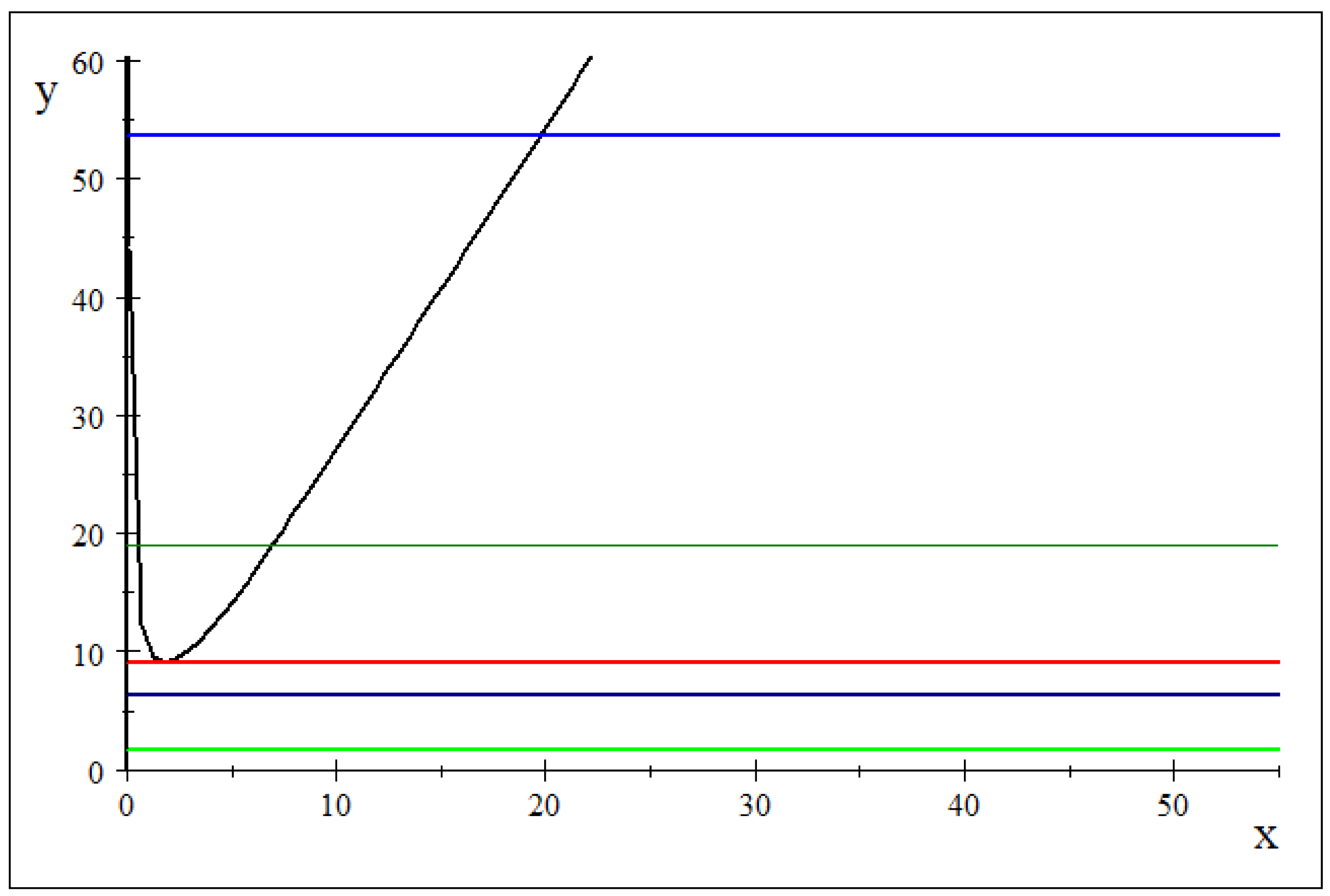
In the graph below, one can see values of ρ 0 , e α 1 which verify condition (24) when α { 1 , 2 , 3 , 4 } . As we can observe, the inequality in (24) is actually very restrictive. Here, the graph of ρ ρ e ρ + 1 e ρ 1 ρ is represented with black, the graph of α e α 1 is represented with light green for α = 1 , with blue for α = 2 , green for α = 3 , and light blue for α = 4 . As we can see, if α < 2.3125 , the inequality in (24) has no solution. In the figure, the line e 2.3125 1 is represented with red.
Figure A1. Ranges of ρ which verify hypothesis (24) and α = 1 in light green, α = 2 in blue, α = 2.3125 in red, α = 3 in green, α = 4 in light blue.
Mathematics 13 03074 g0a1
Hypothesis (24) is not verified either if α ln 10.1 2 . 312 5 or if α > ln 10.1 and ρ has the property that Q < 1 + ρ e ρ + 1 e ρ 1 ρ .
In what follows, we represent both the graph of the series (22) and of the function (A4) for pairs α , ρ which do not verify (24), and we can see that even for such pairs, the series (22) is not constant. Therefore, except for the studied case, this assertion remains a conjecture.
 Remark A2. 
Let the function
t g α , ρ , m , n , t = k = m n e e α t k e 1 + ρ e α t k , m , n 1
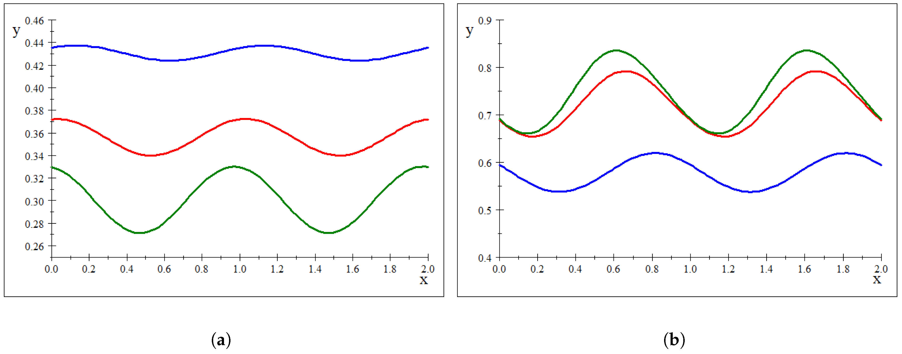
more exactly define partial sums of the series s α , ρ , t . According to the previous remark, if α < 2.3125 = ln 10 , then there is no ρ with the property (24). However, in Figure A2, we can see that t g α , ρ , m , n , t is not constant. In Figure A2a, we have ρ = 1 , m = 2 , n = 10 and α = ln 5 for the blue curve, α = ln 7 for the red one, and α = ln 10 for the green one.
Figure A2b represents the graph of (A10) for α > 2.3125 , or more exactly, α = ln k with k { 11 , 21 , 31 } and ρ such as e α = Q < 1 + ρ e 1 + ρ e ρ 1 ρ (or k < 1 + ρ e 1 + ρ e ρ 1 ρ ). Here, m = 2 , n = 10 as well.
So, in Figure A2, we can see the graph of the function
t g α , ρ , m , n , t = k = m n e e α t k e 1 + ρ e α t k , m , n 1 as a partial sum of the series (22), which is represented for the particular values m = 2 , n = 10 and for three different pairs of values α , ρ .
Figure A2. The graph of the function t g α , ρ , 2 , 10 , t . (a) ( α , ρ ) = ( l n 5 , 1 ) in blue, ( α , ρ ) = ( l n 7 , 1 ) in red, and ( α , ρ ) = ( l n 10 , 1 ) in green. (b) ( α , ρ ) = ( l n 11 , 3 ) in blue, ( α , ρ ) = ( l n 21 , 8 ) in red, and ( α , ρ ) = ( l n 31 , 12 ) in green.
Mathematics 13 03074 g0a2
Remark A3. 
On the other hand, in Figure A3, one can see the graph of the function
t h α , ρ , m , n , t , with
h α , ρ , m , n , t = α k = m n 1 + ρ e α t k e 1 + ρ e α t k e α t k e e α t k ,
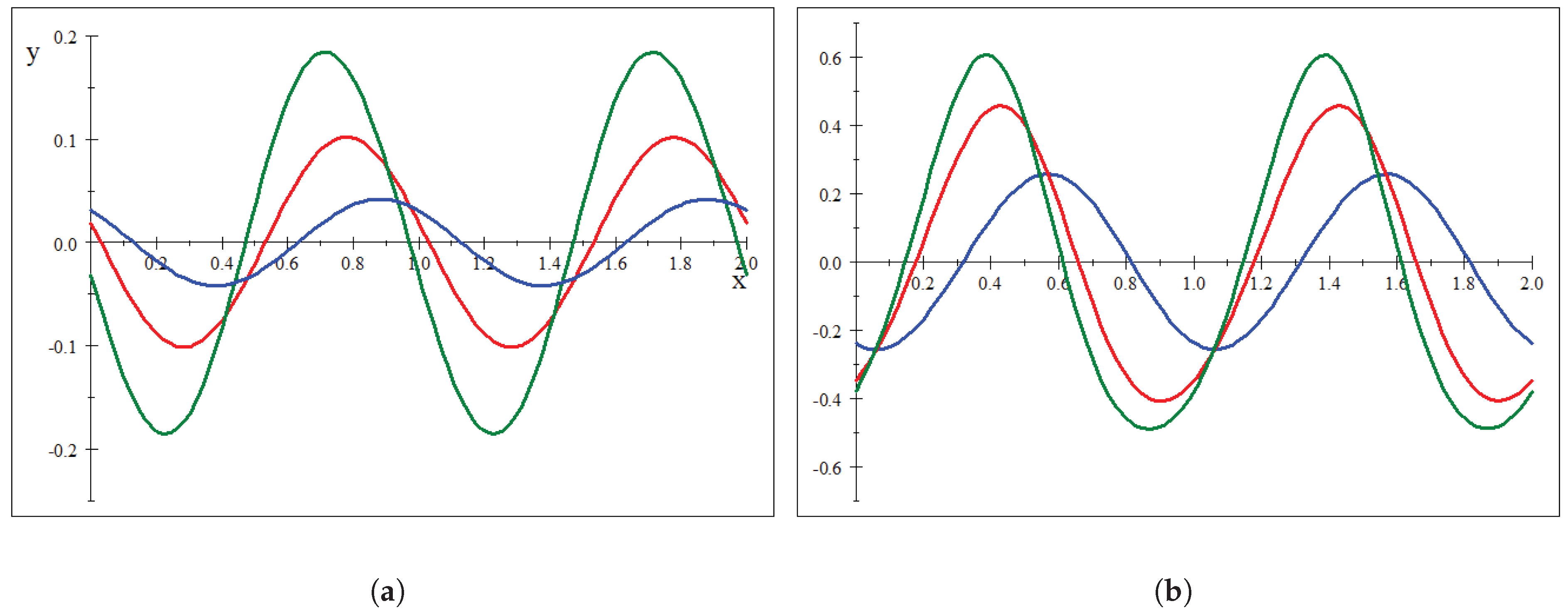
which is a partial sum of the function (23). We chose m = 2 , n = 10 and the same values for the pairs α , ρ as before.
Figure A3. The graph of the function t h ( α , ρ , 2 , 10 , t ) . (a) ( α , ρ ) = ( l n 5 , 1 ) in blue, ( α , ρ ) = ( l n 7 , 1 ) in red, and ( α , ρ ) = ( l n 10 , 1 ) in green. (b) ( α , ρ ) = ( l n 11 , 3 ) in blue, ( α , ρ ) = ( l n 21 , 8 ) in red, and ( α , ρ ) = ( l n 31 , 12 ) in green.
Mathematics 13 03074 g0a3
The graph represented in Figure A3a shows that the derivative is actually positive in a neighborhood of zero if α = ln 5 or α = ln 7 .
Remark A4. 
One can refine this approximation by keeping unchanged a finite number of terms in the series k = 1 w ρ , q k . We have not used that because it is impossible to formulate a condition of type (24).
For instance, we have the following:
E1) Keep w ρ , q unchanged, and we have the following:
k = 1 w ρ , q k = w ρ , q + k = 2 w ρ , q k , and from (A7), we can write k = 1 w ρ , q k < w ρ , q + k = 2 ρ q k ; thus, another approximation for our inequality is
w ρ , q + ρ q 2 1 q < e ρ 1 ρ e 1 + ρ
If w ρ , q + ρ q 2 1 q < e ρ 1 ρ e ρ + 1 , then the derivative of the series (22) calculated in t = 0 is negative too.
E2) For the second case, keep w ρ , q and w ρ , q 2 unchanged, and we have the following:
k = 1 w ρ , q k = w ρ , q + w ρ , q 2 + k = 3 w ρ , q k
Then, the condition
w ρ , q + w ρ , q 2 + ρ q 3 1 q < e ρ 1 ρ e 1 + ρ
is sufficient for the function (A4) to be negative.
Remark A5. 
In order to see the improvements provided by the relations (A11) and (A12), we present the following table. Here E 3 represents the approximation from (A12), E 2 is the approximation from (A11) and E 1 is the approximation from (A9).
Table A1. Intervals for Q given ρ .
E 3 E 2 E 1
ρ = 1 Q > 8.4253 Q > 8.4846 Q > 11.288
ρ = 2 Q > 6.1725 Q > 6.3642 Q > 10.153
ρ = 3 Q > 5.8531 Q > 6.1885 Q > 11.183
ρ = 4 Q > 6.1065 Q > 6.5681 Q > 12.969
If, for instance, ρ = 1 , and we apply (A9) , then the values of Q with the property that (A6) does hold must be greater than 11 . 288 . In comparison, if we apply (A12), we obtain a larger interval for Q and, in consequence, for α as well.
Even if the approximations (A11) and (A12) are less elegant than (A9), they provide more generous sets for the parameters α and ρ .
Proof of Proposition 5. 
Let us have the sets A = k = 1 1 q k , 1 q k + r and B = k = 1 e q k , e q k + r , with q , r 0 , 1 .
Then, a n A = k = 1 1 q k + r n 1 q k n , and a n B = k = 1 e n q k + r e n q k
According to Example 3, we know that lim a n B does not exist. We will prove that A and B have the same nature, and, in consequence, lim a n A does not exist either.
In order to prove that A and B have the same nature, let us check that
lim n k = 1 1 q k + r n 1 q k n e n q k + r e n q k = 0
But, k = 1 1 q k + r n 1 q k n e n q k + r e n q k
k = 1 1 q k + r n e n q k + r + k = 1 1 q k n e n q k
Let us have M k = sup n 1 q k + r n e n q k + r and m k = sup n 1 q k n e n q k , k 1 .
Then, M k = sup n e n q k + r 1 q k + r n = sup n e n q k + r e n ln 1 q k + r and m k = sup n e n q k 1 q k n = sup n e n q k e n ln 1 q k .
For α , β > 0 , it is known that
sup x > 0 e α x e β x 1 min α , β max α , β .
For m k , we have α = q k , β = ln 1 q k ; hence, α < β .
Therefore, m k 1 q k q k + q 2 k 2 + q 3 k 3 + . . . = q k 2 + q 2 k 3 + . 1 + q k 2 + q 2 k 3 + . . . q k , so k = 1 m k < .
For M k , we have α = q k + r , β = ln 1 q k + r ; hence, M k q k + r , and k = 1 M k < .
To conclude, we obtain that the sets A and B have the same nature according to (25)
But this trick does not always hold: see, for instance, the sets already studied, such as
A = k = 1 1 1 k , 1 1 k + r and B = k = 1 e 1 k , e 1 k + r . We know that they have the same nature. However, writing the difference of
a n A = k = 1 1 1 k + r n 1 1 k n and a n B = k = 1 e 1 k + r n e 1 k n , we find that
a n A a n B = k = 1 1 1 k + r n e 1 k + r n 1 1 k n e 1 k n
a n A a n B k = 1 1 1 k + r n e 1 k + r n + k = 1 1 1 k n e 1 k n .
With the same notation as before, we now have
m k = sup n 1 1 k n e 1 k n = sup n e 1 k n e n ln 1 1 k and
M k = sup n 1 1 k + r n e 1 k + r n = sup n e 1 k + r n e n ln 1 1 k + r , k 1 .
We apply (A14): In the case of m k , for β = ln 1 1 k , α = 1 k ,
1 α β = 1 1 k 1 k + 1 2 k 2 + 1 3 k 3 + = 1 2 k + 1 3 k 2 + . . . 1 + 1 2 k + 1 3 k 2 + and the series k = 1 m k is divergent.

References

  1. Barndorff-Nielsen, O.; Sobel, M. On the Distribution of the Number of Admissible Points in a Vector Random Sample. Theory Probab. Appl. 1966, 11, 249–269. [Google Scholar] [CrossRef]
  2. Jacobovic, R.; Zuk, O. A phase transition for the probability of being a maximum among random vectors with general iid coordinates. Stat. Probab. Lett. 2023, 199, 109847. [Google Scholar] [CrossRef]
  3. Bentley, J.L.; Kung, H.T.; Schkolnick, M. On the average number of maxima in a set of vectors and applications. J. ACM 1978, 25, 536–543. [Google Scholar] [CrossRef]
  4. Barbour, A.D.; Xia, A. The number of two-dimensional maxima. Adv. Appl. Probab. 2001, 33, 727–750. [Google Scholar] [CrossRef][Green Version]
  5. Răducan, A.M.; Rădulescu, C.Z.; Rădulescu, M.; Zbăganu, G. On the Probability of Finding Extremes in a Random Set. Mathematics 2022, 10, 1623. [Google Scholar] [CrossRef]
  6. Răducan, A.M.; Zbăganu, G. The Leader Property in Quasi Unidimensional Cases. Mathematics 2022, 10, 4199. [Google Scholar] [CrossRef]
  7. Billingsley, P. Convergence of Probability Measures; John Wiley & Sons, Inc.: New York, NY, USA, 1999. [Google Scholar]
  8. Geiss, H.; Geiss, S. Measure, Probability and Functional Analysis; Springer Nature: Cham, Switzerland, 2025. [Google Scholar]
  9. David, H.A.; Nagaraja, H.N. Order Statistics, 3rd ed.; John Wiley & Sons: New York, NY, USA, 2003. [Google Scholar]
  10. Bartle, R.G. The Elements of Integration and Lebesgue Measure; Wiley Interscience: New York, NY, USA, 1995. [Google Scholar]
  11. Rudin, W. Principles of Mathematical Analysis; International Series in Pure and Applied Mathematics; McGraw-Hill Inc.: Columbus, OH, USA, 1976. [Google Scholar]
Disclaimer/Publisher’s Note: The statements, opinions and data contained in all publications are solely those of the individual author(s) and contributor(s) and not of MDPI and/or the editor(s). MDPI and/or the editor(s) disclaim responsibility for any injury to people or property resulting from any ideas, methods, instructions or products referred to in the content.