Approximation Properties of a Fractional Integral-Type Szász–Kantorovich–Stancu–Schurer Operator via Charlier Polynomials

Abstract

The goal of this manuscript is to introduce a new Stancu generalization of the modified Szász–Kantorovich operator connecting Riemann–Liouville fractional operators via Charlier polynomials. Further, some estimates are calculated as test functions and central moments. In the next section, we investigate some convergence analysis along with the rate of approximations. Moreover, we discuss the order of approximation of a higher-order modulus of smoothness with the help of some moments and establish some convergence results concerning Peetre’s K-functional, Lipschitz-type functions for a newly developed operator $S{K}_{n+p,a}^{v_1,v_2}$. We estimate some results related to Korovkin-, Voronovskaya-, and Grüss–Voronovskaya-type theorems.

1. Introduction

In 1912, Bernstein [1] introduced a sequence of polynomials, now known as Bernstein polynomials, to provide a constructive proof of the Weierstrass approximation theorem using the binomial distribution. These polynomials are defined as

$$\begin{array}{c}\hfill B_n(f;y)=\sum _{l=0}^n{c}_{n,l}\left(y\right)f\left({\displaystyle \frac{l}{n}}\right),y\in [0,1],\end{array}$$

(1)

where f stands for a continuous and bounded function which is presented on $[0,1]$ and Bernstein basis functions $c_{n,l}\left(y\right)=\left(\begin{array}{c}n\\ l\end{array}\right)y^l{(1-y)}^{n-l}$. The sequences of operators in (1) restrict the approximation for continuous functions on $[0,1]$. In order to discuss approximation properties on the unbounded interval $[0,\infty )$, Szász [2] provided modifications to the operators in (1), which has played a significant role in the evolution of operator theory, as follows:

$$\begin{array}{c}\hfill S_n(f;y)=e^{-ny}\sum _{l=0}^{\infty }{\displaystyle \frac{{\left(ny\right)}^l}{l!}}f\left({\displaystyle \frac{l}{n}}\right),n\in \mathbb{N},\mathrm{for}f\in C[0,\infty ).\end{array}$$

(2)

The operators introduced in (2) are positive linear and are limited to approximation results in $C[0,\infty )$. We discuss approximation results in a super class of continuous functions, i.e., the Lebesgue class of measurable functions. Several mathematicians, e.g., Özger et al. [3,4], Ayman Mursaleen et al. [5,6], Braha et al. [7], and Khursheed et al. [8,9], have explored various modifications to improve approximation properties in different functional spaces. Further advancements have been made by researchers such as Khan et al. [10], Acar [11,12], Aslan [13], Mohiuddine et al. [14,15], Mursaleen et al. [16,17], Malik et al. [18], Nasiruzzaman et al. [19,20], and Rao et al. [21,22], among others. These studies have significantly contributed to generalizing Korovkin’s theorem across various domains. Their investigation included the generalization of certain positive linear operators like Phillips-type q-Bernstein, Bernstein–Durrmeyer, and $\lambda$-Schurer–Kantorovich-type operators via various polynomials, the Stancu variant [23,24,25,26], the Summability method (see [27]), and a fractional operator (see [28,29]). Furthermore, they estimated some interesting results concerning a Korovkin-type theorem, Voronoskaya- and Grüss-type theorems, and Grüss inequalities and also performed fine convergence analysis (in both a classical and statistical sense) for the rate of approximations with respect to the modulus of smoothness, etc.

The present work deals with the Stancu generalization of a modified Szász–Kantorovich operator along with Riemann–Liouville fractional operators including Charlier polynomials. Some convergence analysis along with the rate of approximations is discussed. Our investigations mainly focus on the higher-order modulus of smoothness with the help of some moments and establish some convergence results concerning Peetre’s K-functional, Lipschitz-type functions for a newly developed operator $S{K}_{n+p,a}^{v_1,v_2}$. We estimate some results related to Korovkin-, Voronovskaya-, and Grüss–Voronovskaya-type theorems.

Significantly, various generalizations of this operator have been introduced and studied via various polynomials and other operators (see [30,31]). In 2012, Varma and Taşdelen [32] introduced and defined a modified Szász operator by using the Charlier polynomial as follows:

$$\begin{array}{c}\hfill L_n(f;y)=e^{-1}{\left(1-{\displaystyle \frac{1}{a}}\right)}^{(a-1)ny}\sum _{l=0}^{\infty }{\displaystyle \frac{C_l^a(-(a-1)ny)}{l!}}f\left({\displaystyle \frac{l}{n}}\right),\end{array}$$

(3)

where $a>1$, $y\in [0,\infty )$, wherever the generating function is

$$\begin{array}{c}\hfill e^t{\left(1-{\displaystyle \frac{t}{a}}\right)}^v=\sum _{l=0}^{\infty }{C}_l^a{\displaystyle \frac{t^l}{l!}},|t|<a,\end{array}$$

$$\begin{array}{c}\hfill C_l^a\left(u\right)=\sum _{s=0}^l\left(\begin{array}{c}l\\ s\end{array}\right){\left(-u\right)}_s{\left({\displaystyle \frac{l}{a}}\right)}^s,\end{array}$$

(4)

and ${\left(\sigma \right)}_l$ is the Pochhammer symbol or shifted factorial defined by

$$\begin{array}{c}\hfill {\left(\sigma \right)}_l=\left\{\begin{array}{c}1\sigma =0\mathrm{or}l=0,\\ \sigma (\sigma +1)........(\sigma -l+1),l\in \mathbb{N},\end{array}\right.\end{array}$$

where $\sigma \in \mathbb{R}$. In particular, we are motivated by the recent monograph of Ansari et al. [33], where the authors had introduced the Kantorovich generalization of Equation (2), defined as below:

$$Q_{n,b}^{{\mathfrak{T}}_n,{\xi }_n}(f;y)={\xi }_n{e}^{-1}{\left(1-{\displaystyle \frac{1}{a}}\right)}^{(a-1){\mathfrak{T}}_{n}y}\sum _{l=0}^{\infty }{\displaystyle \frac{C_l^a(-(a-1){\mathfrak{T}}_{n}y)}{l!}}{\int }_{{\displaystyle \frac{l}{{\xi }_n}}}^{{\displaystyle \frac{l+1}{{\xi }_n}}}f\left(\theta \right)d\theta$$

(5)

where ${\mathfrak{T}}_n$ and ${\xi }_n$ are the sequence of increasing and unbounded positive numbers such that

$$\begin{array}{c}\hfill \underset{n\to \infty }{lim}{\displaystyle \frac{1}{{\xi }_n}}=0\mathrm{and}{\displaystyle \frac{{\mathfrak{T}}_n}{{\xi }_n}}=1+o\left({\displaystyle \frac{1}{{\xi }_n}}\right),n\to \infty .\end{array}$$

Motivated by all the above work, we introduce a new positive linear operator $S{K}_{n+p,a}^{v_1,v_2}$ on $[0,\infty )$, via the Stancu–Shurer variant $v_1,v_2\in {\mathbb{R}}^{+}$,

$$\begin{array}{cc}\hfill S{K}_{n+p,a}^{v_1,v_2}(f;y)& = \left({\xi }_{n+p}+v_2\right)e^{-1}{\left(1-{\displaystyle \frac{1}{a}}\right)}^{(a-1){\mathfrak{T}}_{n+p}y}\sum _{l=0}^{\infty }{\displaystyle \frac{C_l^a(-(a-1){\mathfrak{T}}_{n+p}y)}{l!}}\hfill \\ \hfill & {\int }_{{\displaystyle \frac{l+v_1}{{\xi }_{n+p}+v_2}}}^{{\displaystyle \frac{l+v_1+1}{{\xi }_{n+p}+v_2}}}f\left(t\right)\hfill \\ \hfill & = e^{-1}{\left(1-{\displaystyle \frac{1}{a}}\right)}^{(a-1){\mathfrak{T}}_{n+p}y}\sum _{l=0}^{\infty }{\displaystyle \frac{C_l^a(-(a-1){\mathfrak{T}}_{n+p}y)}{l!}}\hfill \\ \hfill & {\int }_0^{1}f\left({\displaystyle \frac{t+l+v_1}{{\xi }_{n+p}+v_2}}\right)dt.\hfill \end{array}$$

We can further generalize the above operator with the help of the Riemann–Liouville fractional integral operator for order $\zeta$ as follows:

$$\begin{array}{c}\hfill S{K}_{n+p,a}^{v_1,v_2}(f;y)=Q_{{\mathfrak{T}}_{n+p}y}\sum _{l=0}^{\infty }{\displaystyle \frac{C_l^a(-(a-1){\mathfrak{T}}_{n+p}y)}{l!}}{\int }_0^1{\displaystyle \frac{{(1-t)}^{\zeta -1}}{\mathsf{\Gamma }\left(\zeta \right)}}f\left({\displaystyle \frac{t+l+v_1}{{\xi }_{n+p}+v_2}}\right)dt\end{array}$$

where $Q_{{\mathfrak{T}}_{n+p}y}=e^{-1}{\left(1-{\displaystyle \frac{1}{a}}\right)}^{(a-1){\mathfrak{T}}_{n+p}y}$.

In particular, this operator includes the operators as in Equations (2), (3), and (5).

• For $v_1,v_2=0$, and $\zeta =0$, this operator reduces to the operator defined in [33].
• For ${\mathfrak{T}}_{n+p}={\xi }_{n+p}=n$, the operator is generalized to the operator defined in [30].

Remark 1.

For any $f,g\in C[0,\infty )$ and $a_1,a_2\in \mathbb{R}$, we have

$$\begin{array}{cc}S{K}_{n+p,a}^{v_1,v_2}(a_{1}f+a_{2}g;y)& = Q_{{\mathfrak{T}}_{n+p}y}\sum _{l=0}^{\infty }{\displaystyle \frac{C_l^a(-(a-1){\mathfrak{T}}_{n+p}y)}{l!}}\hfill \\ \hfill & {\int }_0^1{\displaystyle \frac{{(1-t)}^{\zeta -1}}{\mathsf{\Gamma }\left(\zeta \right)}}(a_{1}f+a_{2}g)\left({\displaystyle \frac{t+l+v_1}{{\xi }_{n+p}+v_2}}\right)dt\hfill \\ \hfill & = a_1{Q}_{{\mathfrak{T}}_{n+p}y}\sum _{l=0}^{\infty }{\displaystyle \frac{C_l^a(-(a-1){\mathfrak{T}}_{n+p}y)}{l!}}{\int }_0^1{\displaystyle \frac{{(1-t)}^{\zeta -1}}{\mathsf{\Gamma }\left(\zeta \right)}}f\left({\displaystyle \frac{t+l+v_1}{{\xi }_{n+p}+v_2}}\right)dt\hfill \\ \hfill & +a_2{Q}_{{\mathfrak{T}}_{n+p}y}\sum _{l=0}^{\infty }{\displaystyle \frac{C_l^a(-(a-1){\mathfrak{T}}_{n+p}y)}{l!}}{\int }_0^1{\displaystyle \frac{{(1-t)}^{\zeta -1}}{\mathsf{\Gamma }\left(\zeta \right)}}g\left({\displaystyle \frac{t+l+v_1}{{\xi }_{n+p}+v_2}}\right)dt\hfill \\ \hfill & = a_{1}S{K}_{n+p,a}^{v_1,v_2}(f;y)+a_{2}S{K}_{n+p,a}^{v_1,v_2}(g;y).\hfill \end{array}$$

This implies that the given sequences of operators $S{K}_{n+p,a}^{v_1,v_2}(.;.)$ are a linear operator. Also, for any $f\ge 0$, we must have $S{K}_{n+p,a}^{v_1,v_2}(f;y)\ge 0$, which shows that the sequence of operators is positive.

In the following sections, we examine the convergence rate of operators and their approximation order. Specifically, we discuss the order of approximation of a higher-order modulus of smoothness with the help of some moments and establish some convergence results concerning Peetre’s K functional, Lipschitz-type functions. In the final section, we explore some results related to Korovkin-, Voronovskaya-, and Grüss–Voronovskaya-type theorems.

2. Main Results

In the current section, we estimate some fundamental moments. Before moving towards our main results, we require the following Lemma from [33]:

Lemma 1

([33]). Let $C_l^a\left(u\right)$ be Charlier polynomials’ generating function given by (4). Then, we have

$$\begin{array}{cc}\hfill \sum _{l=0}^{\infty }{\displaystyle \frac{C_l^a(-(a-1){\mathfrak{T}}_{n+p}y)}{l!}}& = e{\left(1-{\displaystyle \frac{1}{a}}\right)}^{-(a-1){\mathfrak{T}}_{n+p}y},\hfill \\ \hfill \sum _{l=0}^{\infty }{\displaystyle \frac{l{C}_l^a(-(a-1){\mathfrak{T}}_{n+p}y)}{l!}}& = e{\left(1-{\displaystyle \frac{1}{a}}\right)}^{-(a-1){\mathfrak{T}}_{n+p}y}(1+{\mathfrak{T}}_{n+p}y),\hfill \end{array}$$

$$\begin{array}{cc}\hfill \sum _{l=0}^{\infty }{\displaystyle \frac{l^2{C}_l^a(-(a-1){\mathfrak{T}}_{n+p}y)}{l!}}& = e{\left(1-{\displaystyle \frac{1}{a}}\right)}^{-(a-1){\mathfrak{T}}_{n+p}y}\hfill \\ \hfill & \left({\mathfrak{T}}_{n+p}^2{y}^2+{\mathfrak{T}}_{n+p}y\left(3+{\displaystyle \frac{1}{a-1}}\right)+2\right),\hfill \\ \hfill \sum _{l=0}^{\infty }{\displaystyle \frac{l^3{C}_l^a(-(a-1){\mathfrak{T}}_{n+p}y)}{l!}}& = e{\left(1-{\displaystyle \frac{1}{a}}\right)}^{-(a-1){\mathfrak{T}}_{n+p}y}({\mathfrak{T}}_{n+p}^3{y}^3+{\mathfrak{T}}_{n+p}^2{y}^2\hfill \\ \hfill & \left(6+{\displaystyle \frac{3}{a-1}}\right)+{\mathfrak{T}}_{n+p}y\left(10+{\displaystyle \frac{6}{a-1}}+{\displaystyle \frac{2}{{(a-1)}^2}}\right)+5),\hfill \\ \hfill \sum _{l=0}^{\infty }{\displaystyle \frac{l^4{C}_l^a(-(a-1){\mathfrak{T}}_{n+p}y)}{l!}}& = e{\left(1-{\displaystyle \frac{1}{a}}\right)}^{-(a-1){\mathfrak{T}}_{n+p}y}\{{\mathfrak{T}}_{n+p}^4{y}^4+{\mathfrak{T}}_{n+p}^3{y}^3\left(10+{\displaystyle \frac{6}{a-1}}\right)\hfill \\ & + {\mathfrak{T}}_{n+p}^2{y}^2\left(6+{\displaystyle \frac{3}{a-1}}\right)+{\mathfrak{T}}_{n+p}^2{y}^2\left(32+{\displaystyle \frac{30}{a-1}}+{\displaystyle \frac{11}{{(a-1)}^2}}\right)\hfill \\ & + {\mathfrak{T}}_{n+p}y\left(37+{\displaystyle \frac{32}{a-1}}+{\displaystyle \frac{20}{{(a-1)}^2}}+{\displaystyle \frac{6}{{(a-1)}^3}}\right)+15\}.\hfill \end{array}$$

Theorem 1.

Suppose that $e_j\left(t\right)=t^j$, for all $t\in [0,\infty )$. Then, we obtain the following identity:

$$\begin{array}{cc}S{K}_{n+p,a}^{v_1,v_2}(e_j;y)=& {\displaystyle \frac{\mathsf{\Gamma }(\zeta +1)}{{({\xi }_{n+p}+v_2)}^j}}{e}^{-1}{\left(1-{\displaystyle \frac{1}{a}}\right)}^{(a-1){\mathfrak{T}}_{n+p}y}\sum _{l=0}^{\infty }{\displaystyle \frac{C_l^a(-(a-1){\mathfrak{T}}_{n+p}y)}{l!}}\hfill \\ & \times \sum _{l=0}^j\left(\begin{array}{c}j\\ l\end{array}\right){(l+v_1)}^l{\displaystyle \frac{\mathsf{\Gamma }(j-l+1)}{\mathsf{\Gamma }(j-l+\zeta +1)}}.\hfill \end{array}$$

(6)

Proof. 

The proof proceeds like this:

$$\begin{array}{cc}\hfill S{K}_{n+p,a}^{v_1,v_2}(e_j;y)& = e^{-1}{\left(1-{\displaystyle \frac{1}{a}}\right)}^{(a-1){\mathfrak{T}}_{n+p}y}\mathsf{\Gamma }(\zeta +1)\sum _{l=0}^{\infty }{\displaystyle \frac{C_l^a(-(a-1){\mathfrak{T}}_{n+p}y)}{l!}}\hfill \\ \hfill & {\int }_0^1{\displaystyle \frac{{(1-t)}^{\zeta -1}}{\mathsf{\Gamma }\left(\zeta \right)}}{\displaystyle \frac{{(t+l+v_1)}^j}{{({\xi }_{n+p}+v_2)}^j}}dt\hfill \\ \hfill & =e^{-1}{\left(1-{\displaystyle \frac{1}{a}}\right)}^{(a-1){\mathfrak{T}}_{n+p}y}{\displaystyle \frac{\mathsf{\Gamma }(\zeta +1)}{\mathsf{\Gamma }\left(\zeta \right){({\xi }_{n+p}+v_2)}^j}}\hfill \\ \hfill & \sum _{l=0}^{\infty }{\displaystyle \frac{C_l^a(-(a-1){\mathfrak{T}}_{n+p}y)}{l!}}{\int }_0^1{(1-t)}^{\zeta -1}{(t+l+v_1)}^{j}dt\hfill \\ \hfill & =e^{-1}{\left(1-{\displaystyle \frac{1}{a}}\right)}^{(a-1){\mathfrak{T}}_{n}y}{\displaystyle \frac{\mathsf{\Gamma }(\zeta +1)}{\mathsf{\Gamma }\left(\zeta \right){({\xi }_{n+p}+v_2)}^j}}\sum _{l=0}^{\infty }{\displaystyle \frac{C_l^a(-(a-1){\mathfrak{T}}_{n}y)}{l!}}\hfill \\ \hfill & {\int }_0^1{(1-t)}^{\zeta -1}\left(\sum _{k=0}^j\left(\begin{array}{c}j\\ l\end{array}\right){(l+v_1)}^l{t}^{j-l}\right)dt\hfill \\ \hfill & =e^{-1}{\left(1-{\displaystyle \frac{1}{a}}\right)}^{(a-1){\mathfrak{T}}_{n+p}y}{\displaystyle \frac{\mathsf{\Gamma }(\zeta +1)}{\mathsf{\Gamma }\left(\zeta \right){({\xi }_{n+p}+v_2)}^j}}\sum _{l=0}^{\infty }{\displaystyle \frac{C_l^a(-(a-1){\mathfrak{T}}_{n+p}y)}{l!}}\hfill \\ \hfill & \sum _{l=0}^j\left(\begin{array}{c}j\\ l\end{array}\right){(l+v_1)}^l{\int }_0^1{(1-t)}^{\zeta -1}{t}^{j-l}dt\hfill \\ \hfill & = e^{-1}{\left(1-{\displaystyle \frac{1}{a}}\right)}^{(a-1){\mathfrak{T}}_{n+p}y}{\displaystyle \frac{\mathsf{\Gamma }(\zeta +1)}{\mathsf{\Gamma }\left(\zeta \right){({\xi }_{n+p}+v_2)}^j}}\sum _{l=0}^{\infty }{\displaystyle \frac{C_l^a(-(a-1){\mathfrak{T}}_{n+p}y)}{l!}}\hfill \\ \hfill & \sum _{l=0}^j\left(\begin{array}{c}j\\ l\end{array}\right){(l+v_1)}^l\beta (\zeta ,j-l+1)\hfill \\ \hfill & = e^{-1}{\left(1-{\displaystyle \frac{1}{a}}\right)}^{(a-1){\mathfrak{T}}_{n+p}y}{\displaystyle \frac{\mathsf{\Gamma }(\zeta +1)}{\mathsf{\Gamma }\left(\zeta \right){({\xi }_{n+p}+v_2)}^j}}\sum _{l=0}^{\infty }{\displaystyle \frac{C_l^a(-(a-1){\mathfrak{T}}_{n+p}y)}{l!}}\hfill \\ \hfill & \sum _{l=0}^j\left(\begin{array}{c}j\\ l\end{array}\right){(l+v_1)}^l{\displaystyle \frac{\mathsf{\Gamma }(j-l+1)}{\mathsf{\Gamma }(j-l+\zeta +1)}}.\hfill \end{array}$$

□

Lemma 2.

We have, by Theorem 1,

$$\begin{array}{cc}\hfill S{K}_{n+p,a}^{v_1,v_2}(1;y)& =1,\hfill \\ \hfill S{K}_{n+p,a}^{v_1,v_2}(t;y)& ={\displaystyle \frac{1}{(\zeta +1)({\xi }_{n+p}+v_2)}}+{\displaystyle \frac{v_1+1}{{\xi }_{n+p}+v_2}}+{\displaystyle \frac{{\mathfrak{T}}_{n+p}}{{\xi }_{n+p}+v_2}}y,\hfill \\ \hfill S{K}_{n+p,a}^{v_1,v_2}(t^2;y)& ={\displaystyle \frac{2}{(\zeta +1)(\zeta +2){({\xi }_{n+p}+v_2)}^2}}+{\displaystyle \frac{v_1^2+2(v_1+1)}{(\zeta +1){({\xi }_{n+p}+v_2)}^2}}+y^2{\displaystyle \frac{{\mathfrak{T}}_{n+p}^2}{{({\xi }_{n+p}+v_2)}^2}}\hfill \\ \hfill & +{\displaystyle \frac{2(v_1+1+{\mathfrak{T}}_{n+p})}{{({\xi }_{n+p}+v_2)}^2}}+{\displaystyle \frac{y}{{({\xi }_{n+p}+v_2)}^2}}\left(2v_1+3+{\displaystyle \frac{1}{a-1}}\right){\mathfrak{T}}_{n+p},\hfill \\ \hfill S{K}_{n+p,a}^{v_1,v_2}(t^3;y)& =\{{\displaystyle \frac{6}{(\zeta +1)(\zeta +2)(\zeta +3){({\xi }_{n+p}+v_2)}^3}}+{\displaystyle \frac{2+2v_1}{(\zeta +1)(\zeta +2){({\xi }_{n+p}+v_2)}^3}}\hfill \\ \hfill & +{\displaystyle \frac{2+2v_1+v_1^2}{(\zeta +1){({\xi }_{n+p}+v_2)}^3}}+{\displaystyle \frac{5+6v_1+3v_1^2+v_1^3}{{({\xi }_{n+p}+v_2)}^3}}\}\hfill \\ \hfill & +y\{{\displaystyle \frac{2}{(\zeta +1)(\zeta +2){({\xi }_{n+p}+v_2)}^3}}+{\displaystyle \frac{(3+\frac{1}{a-1})+2v_1}{(\zeta +1){({\xi }_{n+p}+v_2)}^3}}\hfill \\ \hfill & +{\displaystyle \frac{(10+\frac{6}{a-1}+\frac{2}{{(a-1)}^2})}{{({\xi }_{n+p}+v_2)}^3}}+{\displaystyle \frac{3v_1(3+\frac{1}{a-1})+3}{{({\xi }_{n+p}+v_2)}^3}}\}{\mathfrak{T}}_{n+p}\hfill \\ \hfill & +y^2\{{\displaystyle \frac{2}{(\zeta +1){({\xi }_{n+p}+v_2)}^3}}+{\displaystyle \frac{(6+\frac{3}{a-1})}{(\zeta +1){({\xi }_{n+p}+v_2)}^3}}\hfill \\ \hfill & +{\displaystyle \frac{3v_1}{{({\xi }_{n+p}+v_2)}^3}}\}{\mathfrak{T}}_{n+p}^2+y^3\left\{{\displaystyle \frac{1}{{({\xi }_{n+p}+v_2)}^3}}\right\}{\mathfrak{T}}_{n+p}^3,\hfill \\ \hfill S{K}_{n+p,a}^{v_1,v_2}(t^4;y)& =\{{\displaystyle \frac{24}{(\zeta +1)(\zeta +2)(\zeta +3)(\zeta +4){({\xi }_{n+p}+v_2)}^4}}\hfill \\ \hfill & +{\displaystyle \frac{6+6v_1}{(\zeta +1)(\zeta +2)(\zeta +3){({\xi }_{n+p}+v_2)}^4}}+{\displaystyle \frac{2(2+2v_1+v_1^2)}{(\zeta +1)(\zeta +2){({\xi }_{n+p}+v_2)}^4}}\hfill \\ \hfill & +{\displaystyle \frac{5+6v_1+9v_1^2+v_1^3}{(\zeta +1){({\xi }_{n+p}+v_2)}^4}}+{\displaystyle \frac{15+20v_1+12v_1^2+4v_1^3+v_1^4}{{({\xi }_{n+p}+v_2)}^4}}\}\hfill \\ \hfill & +{\displaystyle \frac{y}{{({\xi }_{n+p}+v_2)}^4}}\{{\displaystyle \frac{3}{(\zeta +1)(\zeta +2)(\zeta +3)}}+{\displaystyle \frac{2(3+\frac{1}{a-1})+4v_1}{(\zeta +1)(\zeta +2)}}\hfill \\ \hfill & +{\displaystyle \frac{3v_1\left(3+\frac{1}{a-1}\right)+3v_1+3v_1^2}{(\zeta +1)}}+\left\{37+{\displaystyle \frac{32}{a-1}}+{\displaystyle \frac{20}{{(a-1)}^2}}+{\displaystyle \frac{6}{{(a-1)}^3}}\right\}\hfill \\ \hfill & +4v_1\left\{10+{\displaystyle \frac{6}{a-1}}+{\displaystyle \frac{2}{{(a-1)}^2}}\right\}\}{\mathfrak{T}}_{n+p}\hfill \\ \hfill & +{\displaystyle \frac{y^2}{{({\xi }_{n+p}+v_2)}^4}}\{{\displaystyle \frac{2}{(\zeta +1)(\zeta +2)}}+{\displaystyle \frac{(6+\frac{3}{a-1})+3v_1}{(\zeta +1)}}+4v_1\left(6+{\displaystyle \frac{3}{a-1}}\right)\hfill \\ \hfill & +6v_1^2+\left(32+{\displaystyle \frac{30}{a-1}}+{\displaystyle \frac{11}{{(a-1)}^2}}\right)\}{\mathfrak{T}}_{n+p}^2\hfill \\ \hfill & +{\displaystyle \frac{y^3}{{({\xi }_{n+p}+v_2)}^4}}\left\{{\displaystyle \frac{1}{\zeta +1}}+4v_1+10+{\displaystyle \frac{6}{a-1}}\right\}{\mathfrak{T}}_{n+p}^3+{\displaystyle \frac{y^4}{{({\xi }_{n+p}+v_2)}^4}}{\mathfrak{T}}_{n+p}^4.\hfill \end{array}$$

Theorem 2.

Suppose that $e_j^{*}\left(t\right)={(t-y)}^j$, for all $t\in [0,\infty )$ and $j\in {\mathbb{N}}_0$ Then, we have the following identity:

$$\begin{array}{cc}\hfill S{K}_{n+p,a}^{v_1,v_2}(e_j^{*};y)& = {\displaystyle \frac{\mathsf{\Gamma }(\zeta +1)}{{({\xi }_{n+p}+v_2)}^j}}{e}^{-1}{\left(1-{\displaystyle \frac{1}{a}}\right)}^{(a-1){\mathfrak{T}}_{n+p}y}\sum _{l=0}^{\infty }{\displaystyle \frac{C_l^a(-(a-1){\mathfrak{T}}_{n+p}y)}{l!}}\hfill \\ \hfill & \sum _{i=0}^j\left(\begin{array}{c}j\\ i\end{array}\right){(-1)}^{j-k}{\left(y({\xi }_{n+p}+v_2)\right)}^{j-i}\hfill \\ \hfill & \sum _{m=0}^i\left(\begin{array}{c}i\\ m\end{array}\right){\displaystyle \frac{{(l+v_1)}^k\left(\mathsf{\Gamma }(i-m+1)\right)}{\mathsf{\Gamma }(i-m+\zeta +1)}}.\hfill \end{array}$$

Proof. 

The proof is similar to that of Theorem 1. □

Using the above Theorem 2, we have the lemma given below:

Lemma 3.

We have estimates

$$\begin{array}{cc}\hfill S{K}_{n+p,a}^{v_1,v_2}({(t-y)}^1;y)& = \left({\displaystyle \frac{{\mathfrak{T}}_{n+p}}{{\xi }_{n+p}+v_2}}-1\right)y+{\displaystyle \frac{1}{(\zeta +1)({\xi }_{n+p}+v_2)}}+{\displaystyle \frac{v_1+1}{{\xi }_{n+p}+v_2}},\hfill \\ \hfill S{K}_{n+p,a}^{v_1,v_2}({(t-y)}^2;y)& = y^2\left\{1-2\left({\displaystyle \frac{{\mathfrak{T}}_{n+p}}{({\xi }_{n+p}+v_2)}}\right)+{\displaystyle \frac{{\mathfrak{T}}_{n+p}^2}{{({\xi }_{n+p}+v_2)}^2}}\right\}\hfill \\ \hfill & +y\{{\displaystyle \frac{-2}{({\xi }_{n+p}+v_2)(\zeta +1)}}-{\displaystyle \frac{2(1+v_1)}{({\xi }_{n+p}+v_2)}}+{\displaystyle \frac{{\mathfrak{T}}_{n+p}\left(3+\frac{1}{a-1}\right)}{{({\xi }_{n+p}+v_2)}^2}}\hfill \\ \hfill & +{\displaystyle \frac{2v_1{\mathfrak{T}}_{n+p}}{{({\xi }_{n+p}+v_2)}^2}}+{\displaystyle \frac{2{\mathfrak{T}}_{n+p}}{{({\xi }_{n+p}+v_2)}^2(\zeta +1)}}\}+\{{\displaystyle \frac{2}{(\zeta +1)(\zeta +2){({\xi }_{n+p}+v_2)}^2}}\hfill \\ \hfill & +{\displaystyle \frac{2(v_1+1)}{(\zeta +1){({\xi }_{n+p}+v_2)}^2}}+{\displaystyle \frac{v_1^2+2(v_1+1)}{{({\xi }_{n+p}+v_2)}^2}}\},\hfill \\ \hfill S{K}_{n+p,a}^{v_1,v_2}({(t-y)}^3;y)& = y^3\left\{-1+{\displaystyle \frac{3{\mathfrak{T}}_{n+p}}{{\xi }_{n+p}+v_2}}-{\displaystyle \frac{3{\mathfrak{T}}_{n+p}^2}{{({\xi }_{n+p}+v_2)}^2}}+{\displaystyle \frac{3{\mathfrak{T}}_{n+p}^3}{{({\xi }_{n+p}+v_2)}^3}}\right\}\hfill \\ \hfill & +y^2\{{\displaystyle \frac{3}{(\zeta +1)({\xi }_{n+p}+v_2)}}+{\displaystyle \frac{3}{{\xi }_{n+p}+v_2}}+{\displaystyle \frac{3v_1}{({\xi }_{n+p}+v_2)}}-{\displaystyle \frac{6{\mathfrak{T}}_{n+p}}{(\zeta +1){({\xi }_{n+p}+v_2)}^2}}\hfill \\ \hfill & -{\displaystyle \frac{3{\mathfrak{T}}_{n+p}\left(3+\frac{1}{a-1}\right)}{{({\xi }_{n+p}+v_2)}^2}}+{\displaystyle \frac{3{\mathfrak{T}}_{n+p}^2}{{({\xi }_{n+p}+v_2)}^3)(\zeta +1)}}+{\displaystyle \frac{3{\mathfrak{T}}_{n+p}^2\left(6+\frac{3}{a-1}+3v_1\right)}{{({\xi }_{n+p}+v_2)}^3)}}\hfill \\ \hfill & -{\displaystyle \frac{6v_1{\mathfrak{T}}_{n+p}}{{({\xi }_{n+p}+v_2)}^2}}\}+y\{{\displaystyle \frac{-6}{(\zeta +1)(\zeta +2){({\xi }_{n+p}+v_2)}^3}}+{\displaystyle \frac{3{\mathfrak{T}}_{n+p}\left(3+\frac{1}{a-1}\right)}{(\zeta +1){({\xi }_{n+p}+v_2)}^3}}\hfill \\ \hfill & +{\displaystyle \frac{6v_1{\mathfrak{T}}_{n+p}}{(\zeta +1){({\xi }_{n+p}+v_2)}^3}}+{\displaystyle \frac{{\mathfrak{T}}_{n+p}\left(10+\frac{6}{a-1}+\frac{2}{{(a-1)}^2}\right)+3v_1^2{\mathfrak{T}}_{n+p}}{{({\xi }_{n+p}+v_2)}^3}}\hfill \\ \hfill & +{\displaystyle \frac{3v_1{\mathfrak{T}}_{n+p}(3+\frac{1}{a-1})}{{({\xi }_{n+p}+v_2)}^3}}\}+{\displaystyle \frac{6}{(\zeta +1)(\zeta +2)(\zeta +3){({\xi }_{n+p}+v_2)}^3}}\hfill \\ \hfill & +\{{\displaystyle \frac{6+6v_1}{(\zeta +1)(\zeta +2){({\xi }_{n+p}+v_2)}^3}}+{\displaystyle \frac{3(2+2v_1+v_1^2)}{(\zeta +1){({\xi }_{n+p}+v_2)}^3}}\hfill \\ \hfill & +{\displaystyle \frac{5+6v_1+3v_1^2+v_1^3}{(\zeta +1){({\xi }_{n+p}+v_2)}^4}}\},\hfill \\ \hfill S{K}_{n+p,a}^{v_1,v_2}({(t-y)}^4;y)& = y^4\{1+{\displaystyle \frac{4{\mathfrak{T}}_{n+p}}{({\xi }_{n+p}+v_2)}}+{\displaystyle \frac{6{\mathfrak{T}}_{n+p}^2}{{({\xi }_{n+p}+v_2)}^2}}-{\displaystyle \frac{4{\mathfrak{T}}_{n+p}^3}{{({\xi }_{n+p}+v_2)}^3}}\hfill \\ \hfill & +{\displaystyle \frac{{\mathfrak{T}}_{n+p}^4}{{({\xi }_{n+p}+v_2)}^3}}\}+y^3\{{\displaystyle \frac{-4}{(\zeta +1){({\xi }_{n+p}+v_2)}^2}}+{\displaystyle \frac{12{\mathfrak{T}}_{n+p}}{(\zeta +1){({\xi }_{n+p}+v_2)}^2}}+{\displaystyle \frac{6{\mathfrak{T}}_{n+p}\left(3+\frac{1}{a-1}\right)}{{({\xi }_{n+p}+v_2)}^2}}\hfill \\ \hfill & +{\displaystyle \frac{-4{\mathfrak{T}}_{n+p}^2\left(6+\frac{3}{a-1}\right)}{{({\xi }_{n+p}+v_2)}^3}}+{\displaystyle \frac{12{\mathfrak{T}}_{n+p}}{{({\xi }_{n+p}+v_2)}^2(\zeta +1)}}-{\displaystyle \frac{4v_1}{{\xi }_{n+p}+v_2}}+{\displaystyle \frac{12v_1{\mathfrak{T}}_{n+p}}{{({\xi }_{n+p}+v_2)}^2}}-{\displaystyle \frac{4}{{\xi }_{n+p}+v_2}}\hfill \\ \hfill & -{\displaystyle \frac{12v_1{\mathfrak{T}}_{n+p}^2}{{({\xi }_{n+p}+v_2)}^3}}+{\displaystyle \frac{4{\mathfrak{T}}_{n+p}^3}{{({\xi }_{n+p}+v_2)}^4(\zeta +1)}}+{\displaystyle \frac{{\mathfrak{T}}_{n+p}^3\left(10+\frac{6}{a-1}\right)}{{({\xi }_{n+p}+v_2)}^4}}+{\displaystyle \frac{4v_1{\mathfrak{T}}_{n+p}^3}{{({\xi }_{n+p}+v_2)}^4}}\}\hfill \\ \hfill & +y^2\{{\displaystyle \frac{12}{(\zeta +1)(\zeta +2){({\xi }_{n+p}+v_2)}^2}}+{\displaystyle \frac{12+12v_1}{(\zeta +1){({\xi }_{n+p}+v_2)}^2}}+{\displaystyle \frac{12+12v_1}{{({\xi }_{n+p}+v_2)}^2}}\hfill \\ \hfill & +{\displaystyle \frac{6v_1^2}{{({\xi }_{n+p}+v_2)}^2}}-{\displaystyle \frac{24{\mathfrak{T}}_{n+p}}{{({\xi }_{n+p}+v_2)}^3(\zeta +1)(\zeta +2)}}+{\displaystyle \frac{12{\mathfrak{T}}_{n+p}^2}{{({\xi }_{n+p}+v_2)}^4(\zeta +1)(\zeta +2)}}\hfill \\ \hfill & +{\displaystyle \frac{-12\left(3+\frac{1}{a-1}\right)-24{\mathfrak{T}}_{n+p}}{{({\xi }_{n+p}+v_2)}^3(\zeta +1)}}+{\displaystyle \frac{-4{\mathfrak{T}}_{n+p}\left(10+\frac{6}{a-1}+\frac{2}{{(a-1)}^2}\right)}{{({\xi }_{n+p}+v_2)}^3}}-{\displaystyle \frac{12v_1^2{\mathfrak{T}}_{n+p}}{{({\xi }_{n+p}+v_2)}^3}}\hfill \\ \hfill & -{\displaystyle \frac{12v_1{\mathfrak{T}}_{n+p}\left(3+\frac{1}{a-1}\right)}{{({\xi }_{n+p}+v_2)}^3}}-{\displaystyle \frac{12\left(3+\frac{1}{a-1}\right)-24{\mathfrak{T}}_{n+p}}{{({\xi }_{n+p}+v_2)}^3(\zeta +1)}}+{\displaystyle \frac{12{\mathfrak{T}}_{n+p}^2}{{({\xi }_{n+p}+v_2)}^4(\zeta +1)(\zeta +2)}}\hfill \\ \hfill & +{\displaystyle \frac{4{\mathfrak{T}}_{n+p}^2\left(6+\frac{3}{a-1}+3v_1\right)}{{({\xi }_{n+p}+v_2)}^4(\zeta +1)}}+{\displaystyle \frac{{\mathfrak{T}}_{n+p}^2\left(32+\frac{30}{a-1}+\frac{11}{{(a-1)}^2}+24v_1+\frac{12v_1}{a-1}\right)+6v_1^2}{{({\xi }_{n+p}+v_2)}^4}}\hfill \\ \hfill & +y\{{\displaystyle \frac{-24}{(\zeta +1)(\zeta +2)(\zeta +1){({\xi }_{n+p}+v_2)}^3}}+{\displaystyle \frac{24+24v_1}{(\zeta +1)(\zeta +2){({\xi }_{n+p}+v_2)}^3}}\hfill \\ \hfill & -{\displaystyle \frac{20+24v_{1}2v_1^2+4v_1^3}{{({\xi }_{n+p}+v_2)}^3}}-{\displaystyle \frac{24+24v_1+12v_1^2}{{({\xi }_{n+p}+v_2)}^3(\zeta +1)}}+{\displaystyle \frac{12{\mathfrak{T}}_{n+p}\left(3+\frac{1}{a-1}\right)}{{({\xi }_{n+p}+v_2)}^4(\zeta +1)(\zeta +2)}}\hfill \\ \hfill & +{\displaystyle \frac{24{\mathfrak{T}}_{n+p}}{{({\xi }_{n+p}+v_2)}^4(\zeta +1)(\zeta +2)(\zeta +3)}}-{\displaystyle \frac{24v_1{\mathfrak{T}}_{n+p}}{{({\xi }_{n+p}+v_2)}^3(\zeta +1)}}\hfill \\ \hfill & +{\displaystyle \frac{4{\mathfrak{T}}_{n+p}\left(10+\frac{6}{a-1}+\frac{2}{{(a-1)}^2}+9v_1+\frac{9v_1}{a-1}+3v_1^2\right)}{{({\xi }_{n+p}+v_2)}^4(\zeta +1)}}+{\displaystyle \frac{{\mathfrak{T}}_{n+p}\left(\frac{32}{a-1}+\frac{20}{{(a-1)}^2}\right)}{{({\xi }_{n+p}+v_2)}^4}}\hfill \\ \hfill & +{\displaystyle \frac{{\mathfrak{T}}_{n+p}\left(37+\frac{6}{{(a-1)}^3}+4v_1(10+\frac{6}{a-1}+\frac{2}{{(a-1)}^2}+6v_1^2\left(3+\frac{1}{a-1}\right)+4v_1^3\right)}{{({\xi }_{n+p}+v_2)}^4}}\hfill \\ \hfill & +{\displaystyle \frac{24}{{({\xi }_{n+p}+v_2)}^4(\zeta +1)(\zeta +2)(\zeta +3)(\zeta +4)}}+{\displaystyle \frac{24+24v_1+12v_1^2}{{({\xi }_{n+p}+v_2)}^4(\zeta +1)(\zeta +2)}}\hfill \\ \hfill & {\displaystyle \frac{24+24v_1}{{({\xi }_{n+p}+v_2)}^4(\zeta +1)(\zeta +2)(\zeta +3)}}+{\displaystyle \frac{20+24v_1+12v_1^2+4v_1^3}{{({\xi }_{n+p}+v_2)}^4(\zeta +1)}}\hfill \\ \hfill & +{\displaystyle \frac{15+20v_1+12v_1^2+4v_1^3+v_1^4}{{({\xi }_{n+p}+v_2)}^4}}\}.\hfill \end{array}$$

Proof. 

In light of Lemma 2 and the property of linearity, we have

$$\begin{array}{ccc}\hfill S{K}_{n+p,a}^{v_1,v_2}({(t-y)}^1;y)& \hfill =\hfill & S{K}_{n+p,a}^{v_1,v_2}(t;y)-yS{K}_{n+p,a}^{v_1,v_2}(1;y),\hfill \\ \hfill S{K}_{n+p,a}^{v_1,v_2}({(t-y)}^2;y)& \hfill =\hfill & S{K}_{n+p,a}^{v_1,v_2}(t^2;y)-2yS{K}_{n+p,a}^{v_1,v_2}(t;y)+y^{2}S{K}_{n+p,a}^{v_1,v_2}(1;y),\hfill \\ \hfill S{K}_{n+p,a}^{v_1,v_2}({(t-y)}^3;y)& \hfill =\hfill & S{K}_{n+p,a}^{v_1,v_2}(t^3;y)-3yS{K}_{n+p,a}^{v_1,v_2}(t^2;y)+3y^{2}S{K}_{n+p,a}^{v_1,v_2}(t;y)\hfill \\ \hfill & \hfill \hfill & -y^{3}S{K}_{n+p,a}^{v_1,v_2}(1;y),\hfill \\ \hfill S{K}_{n+p,a}^{v_1,v_2}({(t-y)}^4;y)& \hfill =\hfill & S{K}_{n+p,a}^{v_1,v_2}(t^4;y)-4yS{K}_{n+p,a}^{v_1,v_2}(t^3;w)\hfill \\ \hfill & \hfill \hfill & +6y^{2}S{K}_{n+p,a}^{v_1,v_2}(t^2;y)-4y^{3}S{K}_{n+p,a}^{v_1,v_2}(t;y)\hfill \\ \hfill & \hfill \hfill & +y^{4}S{K}_{n+p,a}^{v_1,v_2}(1;y),\hfill \end{array}$$

which completes the desired proof. □

3. Convergence Analysis of ${\mathit{SK}}_{\mathit{n}+\mathit{p},\mathit{a}}^{{\mathit{v}}_{\mathit{1}},{\mathit{v}}_{\mathit{2}}}$

Theorem 3.

Suppose that $f\in C[0,\infty )=\varsigma$ (say). Then,

$$\begin{array}{c}\hfill \underset{n\to \infty }{lim}S{K}_{n+p,a}^{v_1,v_2}(f;y)=f\left(y\right),\end{array}$$

uniformly on$[0,\infty )$.

Proof. 

The proof is obvious from Lemma 2 that ${lim}_{n\to \infty }S{K}_{n+p,a}^{v_1,v_2}(e_j;y)=y^j,$ for $j=0,1,2.$ Hence, by the Bohman and Korovkin theorem [34], we achieve our required result, i.e.,

$$\begin{array}{c}\hfill \underset{n\to \infty }{lim}S{K}_{n+p,a}^{v_1,v_2}(f;y)=f\left(y\right).\end{array}$$

□

Now, we investigate some rates of approximation via the modulus of smoothness associated with the step weight function $\gamma$. Before proceeding further, we require the following terminology from [23,35]. By moduli of smoothness of order r,

$${\omega }_r^{\gamma }(g;\delta )\equiv \underset{0<h\le \delta }{sup}{\parallel {\mathsf{\Delta }}_{h\gamma \left(y\right)}^{r}g\parallel }_{\zeta }$$

whereas $\delta >0$, $\gamma \left(y\right)=\sqrt{y(1+y)}$ is the step weight function on $[0,\infty )$, and

$$\begin{array}{c}\hfill {\mathsf{\Delta }}_{h\gamma \left(y\right)}^{r}g\left(y\right)=\sum _{i=0}^r{(-1)}^i\left({\displaystyle \genfrac{}{}{0pt}{}{r}{i}}\right)f\left(y+\left({\displaystyle \frac{r}{2}}-i\right)h\gamma \left(y\right)\right).\end{array}$$

Furthermore, Peetre’s K-functional on $\zeta$, associated with the step weight function $\gamma$, is defined as in [36]:

$$\begin{array}{c}\hfill K_{r,\gamma }(g;{\delta }^r)=\underset{g^{*}\in \zeta }{inf}\left\{\parallel g-g^{*}{\parallel }_{\zeta }+{\delta }^r{\parallel {\gamma }^2{\left(g^{*}\right)}^{\prime \prime }\parallel }_{\zeta }\right\}\end{array}$$

where $g^{*}$ is differentiable $r-1$ times and absolutely continuous in every finite interval $[a,b]\subset [0,\infty )$.

Theorem 4

([36], Theorem 2.1.1). For any $g\in C[0,\infty )$, there exists some positive constant M and $t_0$, such that

$$M^{-1}{\omega }_r^{\gamma }(g;\delta )\le K_{r,\gamma }(g;{\delta }^r)\le M{\omega }_r^{\gamma }(g;\delta ).$$

Theorem 5.

Suppose that γ is any step weight function and $l\in \varsigma$. Then, we have the following estimation for $S{K}_{n+p,a}^{v_1,v_2}$:

$$|S{K}_{n+p,a}^{v_1,v_2}(l;y)-l\left(y\right)|\le M{w}_r^{\gamma }\left(l;\sqrt{{\displaystyle \frac{{\varphi }_{r+1}{\left(y\right)}^{r+1}+{\psi }_{r+1}\left(y\right)}{4{\gamma }^{r+1}\left(y\right)}}}+w\left(l;{\displaystyle \frac{{\varphi }_r\left(y\right)}{{\gamma }^{r+1}\left(y\right)}}\right)\right).$$

Proof. 

Let us consider the auxiliary operator

$$\mathsf{\Xi }(l;y)=l\left(y\right)+S{K}_{n+p,a}^{v_1,v_2}(l\left(t\right);y)-l(S{K}_{n+p,a}^{v_1,v_2}{(t-y)}^r;y){+y)}^{{\displaystyle \frac{1}{r}}},$$

(7)

where $l\in C_{r+1}\left({\mathbb{R}}^{+}\right)$, and if $l\left(t\right)$ is any polynomial, then $r=\mathrm{Degree}\mathrm{of}l\left(t\right)$. Obviously,

$$\begin{array}{c}\hfill \mathsf{\Xi }(1;y)=1,\mathsf{\Xi }(t;y)=y,\mathsf{\Xi }((t-y);y)=0,\cdots ,\mathsf{\Xi }({(t-y)}^r;y)=0.\end{array}$$

Suppose that $y\in {\mathbb{R}}_0^{+}$ and $l\in Cr+1\left({\mathbb{R}}_0^{+}\right)$. Then, applying Taylor’s series expansion for l, up to the ${(r+1)}^{th}$ term, we obtain

$$l\left(t\right)=l\left(y\right)+(t-y){\displaystyle \frac{l^{\prime }\left(y\right)}{1!}}+{(t-y)}^2{\displaystyle \frac{l^{\prime \prime }\left(y\right)}{2!}}+\cdots +{(t-y)}^r{\displaystyle \frac{l^r\left(y\right)}{r!}}+{\int }_y^t{\displaystyle \frac{{(t-z)}^r}{r!}}{l}^{r+1}\left(z\right)dz.$$

Now, applying the operator $S{K}_{n+p,a}^{v_1,v_2}$ on both sides,

$$\mathsf{\Xi }(t;y)=l\left(y\right)+\mathsf{\Xi }\left({\int }_y^t{\displaystyle \frac{{(t-z)}^r}{r!}}{l}^{r+1}\left(z\right)dz;y\right).$$

(8)

Moreover,

$$\begin{array}{cc}\hfill \mathsf{\Xi }(h;y)=h\left(y\right)& + S{K}_{n+p,a}^{v_1,v_2}\left({\int }_y^t{\displaystyle \frac{{(t-z)}^r}{r!}}{l}^{r+1}\left(z\right)dz;y\right)\hfill \\ \hfill & -\left({\mathsf{\int }}_y^{{\mathsf{\Phi }}_r\left(y\right)+y}{\displaystyle \frac{({\mathsf{\Phi }}_r\left(y\right)+y){-z)}^r}{r!}}{l}^{r+1}\left(z\right)dz;y\right).\hfill \end{array}$$

This implies

$$\begin{array}{cc}\hfill |\mathsf{\Xi }(h;y)-h\left(y\right)|& \le S{K}_{n+p,a}^{v_1,v_2}\left({\mathsf{\int }}_y^t{\displaystyle \frac{{(t-z)}^r}{r!}}{h}^{r+1}\left(z\right)dz;y\right)\hfill \\ \hfill & -\left({\mathsf{\int }}_y^{{\mathsf{\Phi }}_r\left(y\right)+y}{\displaystyle \frac{({\mathsf{\Phi }}_r\left(y\right)+y){-z)}^r}{r!}}{l}^{r+1}\left(z\right)dz;y\right)\hfill \\ \hfill & \le \parallel {\gamma }^{r+1}{h}^{r+1}{\parallel }_{\omega }S{K}_{n+p,a}^{v_1,v_2}\left({\mathsf{\int }}_y^t{\displaystyle \frac{{(t-z)}^r}{{\gamma }^{r+1}\left(y\right)r!}}{h}^{r+1}\left(z\right)dz;y\right)\hfill \\ \hfill & +\parallel {\gamma }^{r+1}{h}^{r+1}{\parallel }_{\omega }\left({\mathsf{\int }}_y^{{\mathsf{\Phi }}_r\left(y\right)+y}{\displaystyle \frac{({\mathsf{\Phi }}_r\left(y\right)+y){-z)}^r}{r!}}{l}^{r+1}\left(z\right){\displaystyle \frac{dz}{{\gamma }^{r+1}\left(y\right)}};y\right)\hfill \\ \hfill & \le {\gamma }^{r+1}\left(y\right)\parallel {\gamma }^{r+1}{h}^{r+1}\parallel \omega \left(S{K}_{n+p,a}^{v_1,v_2}{(t-y)}^{r+1};y\right)+{\parallel {\gamma }^{r+1}{h}^{r+1}\parallel }_{\omega }{\left({\mathsf{\Phi }}_r\left(y\right)\right)}^{r+1}.\hfill \end{array}$$

Moreover, $\mathsf{\Xi }(l;y)\le 3\parallel l\parallel$. Now,

$$\begin{array}{cc}\hfill |\mathsf{\Xi }(l;y)-l(y)|& \le |\mathsf{\Xi }(l;y)-l\left(y\right)+l({\mathsf{\Phi }}_r\left(y\right)+y)-l\left(y\right)|\hfill \\ \hfill & \le \mathsf{\Xi }(l-h;y)+|\mathsf{\Xi }(h;y)-h(y)|+|h(y)-l(y)|\hfill \\ \hfill & +|l({\mathsf{\Phi }}_r\left(y\right)+y)-l\left(y\right)|\hfill \\ \hfill & \le 4\parallel l-h\parallel +\parallel {\gamma }^{-(r+1)}{\left(y\right)\parallel }_{\omega }\left({\mathsf{\Phi }}_{r+1}\left(y\right)+{\psi }_{r+1}\left(y\right)\right)\hfill \\ \hfill & \le 4K_{r+1,\gamma }\left(l;{\displaystyle \frac{{\mathsf{\Phi }}_{r+1}\left(y\right)+{\psi }_{r+1}\left(y\right)}{4{\gamma }^{r+1}\left(y\right)}}\right)\hfill \end{array}$$

There exists some constant $M>0$, such that

$$\begin{array}{c}\hfill |\mathsf{\Xi }(l;y)-l\left(y\right)|\le M{\omega }_{\gamma }^{r+1}\left(l;{\displaystyle \frac{{\mathsf{\Phi }}_{r+1}\left(y\right)+{\psi }_{r+1}\left(y\right)}{4{\gamma }^{r+1}\left(y\right)}}\right).\end{array}$$

Again, from the modulus of smoothness of first order, we get

$$|({\mathsf{\Phi }}_r\left(y\right)+y)-l\left(y\right)|=|l({\mathsf{\Phi }}_r\left(y\right)+y)-l\left(y\right)|\le \omega \left(l;{\displaystyle \frac{{\mathsf{\Phi }}_r\left(y\right)}{{\gamma }^{r+1}\left(y\right)}}\right).$$

Upon combining all the above inequalities, we get

$$\begin{array}{cc}\hfill |S{K}_{n+p,a}^{v_1,v_2}(l;y)-l\left(y\right)|& \le |\mathsf{\Xi }(l;y)-l\left(y\right)|+|l({\mathsf{\Phi }}_r\left(y\right)+y)-l\left(y\right)|\hfill \\ & \le \mathsf{\Xi }(l-h;y)+|\mathsf{\Xi }(h;y)-h(y)|+|h(y)-l(y)|\hfill \\ & +|l({\mathsf{\Phi }}_r\left(y\right)+y)-l\left(y\right)|\hfill \\ & \le M{w}_r^{\gamma }\left(l;\sqrt{{\displaystyle \frac{{\varphi }_{r+1}{\left(y\right)}^{r+1}+{\psi }_{r+1}\left(y\right)}{4{\gamma }^{r+1}\left(y\right)}}}+w\left(l;{\displaystyle \frac{{\varphi }_r\left(y\right)}{{\gamma }^{r+1}\left(y\right)}}\right)\right).\hfill \end{array}$$

□

Now, some local direct approximations are estimated with the help of the Lipschitz-type maximal function. Let us recall a few basic definitions from [23,37]:

$$\begin{array}{c}\hfill Li{p}_M\left(\kappa \right)=\left\{f\in C[0,\infty ):|f\left(t\right)-f\left(y\right)|\le M{\displaystyle \frac{{|t-y|}^{\kappa }}{{({\alpha }_1{y}^2+{\alpha }_{2}y+t)}^{\frac{\kappa }{2}}}},\right\}\end{array}$$

for all $t,y\in [0,\infty )$, ${\alpha }_1,{\alpha }_2>0$, $M>0$, and $\kappa \in (0,1]$.

Theorem 6.

Let $f\in Li{p}_M\left(\kappa \right)$. Then, for every $\tau \in (0,1]$, we have the following inequality:

$$\begin{array}{c}\hfill |S{K}_{n+p,a}^{v_1,v_2}(f;y)-f\left(y\right)|\le M\sqrt[6]{{\displaystyle \frac{{\left[{\varphi }_{n,a}\left(y\right)\right]}^{\tau }}{{[{\alpha }_1{y}^2+{\alpha }_{2}y]}^{3\tau }}}}.\end{array}$$

where $M>0$, ${\alpha }_1,{\alpha }_2\in (0,\infty )$, $0<\tau \le 1$, and ${\varphi }_{n,a}\left(y\right)=S{K}_{n+p,a}^{v_1,v_2}{(|t-y|}^6;y)$.

Proof. 

Without loss of generality, we obtain

$$\begin{array}{c}\hfill |S{K}_{n+p,a}^{v_1,v_2}(f;y)|\le |S{K}_{n+p,a}^{v_1,v_2}\left(f\left(t\right)-f\left(y\right)\right);y)|+|f\left(y\right)||S{K}_{n+p,a}^{v_1,v_2}(1;y)-1|\end{array}$$

Again, from the Lipschitz maximal function, we get

$$\begin{array}{cc}\hfill |S{K}_{n+p,a}^{v_1,v_2}(f;y)-f\left(y\right)|& \le S{K}_{n+p,a}^{v_1,v_2}\left({\displaystyle \frac{{M|t-y|}^{\tau }}{{({\alpha }_1{y}^2+{\alpha }_{2}y+t)}^{\frac{\tau }{2}}}};y\right)\hfill \\ \hfill & \le MS{K}_{n+p,a}^{v_1,v_2}\left({\displaystyle \frac{{|t-y|}^{\tau }}{{({\alpha }_1{y}^2+{\alpha }_{2}y)}^{\frac{\tau }{2}}}};y\right).\hfill \end{array}$$

Applying Hölder’s inequality in the above inequality,

$$\begin{array}{cc}\hfill |S{K}_{n+p,a}^{v_1,v_2}(f;y)-f\left(y\right)|& \le MS{K}_{n+p,a}^{v_1,v_2}{\left({\displaystyle \frac{{|t-y|}^6}{{({\alpha }_1{y}^2+{\alpha }_{2}y)}^3}};y\right)}^{{\displaystyle \frac{\tau }{6}}}{\left(S{K}_{n+p,a}^{v_1,v_2}(1;y)\right)}^{{\displaystyle \frac{6-\tau }{6}}}\hfill \\ \hfill & \le M{\left({\alpha }_1{y}^2+{\alpha }_{2}y\right)}^{-{\displaystyle \frac{\tau }{2}}}{\left\{S{K}_{n+p,a}^{v_1,v_2}{(|t-y|}^6;y)\right\}}^{{\displaystyle \frac{\tau }{6}}}\hfill \\ \hfill & \le M\sqrt[6]{{\displaystyle \frac{{\left[{\varphi }_{n,a}\left(y\right)\right]}^{\tau }}{{[{\alpha }_1{y}^2+{\alpha }_{2}y]}^{3\tau }}}}\hfill \end{array}$$

where ${\varphi }_{n,a}\left(y\right)=S{K}_{n+p,a}^{v_1,v_2}{(|t-y|}^6;y).$ □

4. Voronovskaya- and Grüss–Vororonovskaya-Type Estimates

In this section, we present certain remarks and theorems for the newly positive linear operator $S{K}_{n+p,a}^{v_1,v_2}$

Theorem 7.

We deduce

$$\begin{array}{c}\hfill \underset{n\to \infty }{lim}n(S{K}_{n+p,a}^{v_1,v_2}(f;y)-f\left(y\right))\le \underset{n\to \infty }{lim}n\{S{K}_{n+p,a}^{v_1,v_2}((\eta -y);y)h^{\prime }\left(y\right)\\ +S{K}_{n+p,a}^{v_1,v_2}({(\eta -y)}^2;y){\displaystyle \frac{h^{\prime \prime }\left(y\right)}{2}}+\cdots +{\displaystyle \frac{S{K}_{n+p,a}^{v_1,v_2}({(\eta -y)}^r;y)}{r!}}{f}^r\left(y\right)\}.\hfill \end{array}$$

Proof. 

Suppose that $h\in \varsigma$. Then, from Taylor’s series expansion up to the r-th term, we achieve the following:

$$\begin{array}{c}h\left(\eta \right)=h\left(y\right)+(\eta -y)h^{\prime }\left(y\right)+{(\eta -y)}^2{\displaystyle \frac{h^{\prime \prime }\left(y\right)}{2!}}+\cdots +{(\eta -y)}^r{\displaystyle \frac{h^r\left(y\right)}{r!}}\\ \hfill +{(\eta -y)}^r\Im (\eta ,y),\end{array}$$

(9)

where $\Im (\eta ,y)\to 0$, as $\eta \to y$. Applying the operator $S{K}_{n+p,a}^{v_1,v_2}$, we have

$$\begin{array}{cc}\hfill S{K}_{n+p,a}^{v_1,v_2}(h\left(\eta \right);y)& = h\left(y\right)+S{K}_{n+p,a}^{v_1,v_2}((\eta -y)h^{\prime }\left(y\right);y)+S{K}_{n+p,a}^{v_1,v_2}({(\eta -y)}^2;y){\displaystyle \frac{h^{\prime \prime }\left(y\right)}{2!}}\hfill \\ \hfill & +\cdots +S{K}_{n+p,a}^{v_1,v_2}({(\eta -y)}^r;y){\displaystyle \frac{h^r\left(y\right)}{r!}}+S{K}_{n+p,a}^{v_1,v_2}({(\eta -y)}^r\Im (\eta ,y);y).\hfill \end{array}$$

Again, from the Cauchy–Schwartz inequality, we have

$$S{K}_{n+p,a}^{v_1,v_2}({(\eta -y)}^r\Im (\eta ,y);y)\le \sqrt{S{K}_{n+p,a}^{v_1,v_2}(\Im {(\eta ,y)}^2;y)}\times \sqrt{S{K}_{n+p,a}^{v_1,v_2}({(\eta -y)}^{2r};y)}.$$

It is pertinent to note here that

$$\begin{array}{c}\hfill \underset{n\to \infty }{lim}\left(S{K}_{n+p,a}^{v_1,v_2}(\Im {(\eta ,y)}^2;y)\right)=0.\end{array}$$

This implies that

$$\underset{n\to \infty }{lim}nS{K}_{n,a}^{v_1,v_2}({(\eta -y)}^r\Im (\eta ,y);y)=0.$$

Therefore, we estimate the following result:

$$\begin{array}{c}\underset{n\to \infty }{lim}n\left\{S{K}_{n+p,a}^{v_1,v_2}(h;y)-h\left(y\right)\right\}=\{S{K}_{n+p,a}^{v_1,v_2}((\eta -y);y)h^{\prime }\left(y\right)\hfill \\ \hfill +S{K}_{n+p,a}^{v_1,v_2}({(\eta -y)}^2;y){\displaystyle \frac{h^{\prime \prime }\left(y\right)}{2}}+\cdots +{\displaystyle \frac{S{K}_{n+p,a}^{v_1,v_2}({(\eta -y)}^r;y)}{r!}}{f}^r\left(y\right)\}.\end{array}$$

□

Remark 2.

It can be easily observed that

$$\begin{array}{c}\hfill S{K}_{n+p,a}^{v_1,v_2}({(t-y)}^2;y)\ge {\displaystyle \frac{1}{{({\xi }_{n+p}+v_2)}^2}}{\displaystyle \frac{(v_1+3)(v_1+2)}{3}}.\end{array}$$

Remark 3.

Now, we have the immediate result that

$$\begin{array}{c}\hfill S{K}_{n+p,a}^{v_1,v_2}({(t-y)}^3;y)\le {\displaystyle \frac{n{\mathfrak{P}}_1(v_1,v_2,a)+{\mathfrak{P}}_2(v_1,v_2,a)}{{({\xi }_{n+p}+v_2)}^3}};\end{array}$$

where

$$\begin{array}{c}\hfill {\mathfrak{P}}_1(v_1,v_2,a)={\displaystyle \frac{a^2(-3v_2+15v_1+3v_1^2+19)+a(3v_2-27v_1-6v_1^2-29)}{{(a-1)}^2}}\end{array}$$

and

$$\begin{array}{ccc}\hfill {\mathfrak{P}}_2(v_1,v_2,a)& =& {\displaystyle \frac{3v_1^2+2v_1+12}{{(a-1)}^2}}.\hfill \end{array}$$

Also,

$$\begin{array}{ccc}\hfill S{K}_{n+p,a}^{v_1,v_2}({(t-y)}^4;y)& <& {\displaystyle \frac{n{t}_1+n{t}_2(v_1,v_2,a)+t_3(v_1,v_2)}{{(n+v_2)}^2}},\hfill \end{array}$$

where $t_1$, $t_2$, and $t_3$ are the constants depending upon $v_1,v_2$, and a.

For simplicity, we take ${\mathfrak{T}}_{n+p}={\xi }_n=n$ and restrict our domain from $[0,\infty )$ to $[0,1]$, in further sections.

Theorem 8.

Let us assume that $f\in C[0,1]$, and $f^{\prime }$, $f^{\prime \prime }$ exist in $[0,1]$. Then, we establish the following estimation:

$$\begin{array}{cc}\hfill |n(S{K}_{n+p,a}^{v_1,v_2}(f;y)-f\left(y\right))& - S{K}_{n+p,a}^{v_1,v_2}(z-y;y)f^{\prime }\left(y\right)\hfill \\ \hfill & - {\displaystyle \frac{1}{2}}S{K}_{n+p,a}^{v_2,v_2}({(z-y)}^2;y)f^{\prime \prime }\left(y\right)|\hfill \\ \hfill & \le K^{*}\left\{w_1\left(f^{\prime },{\displaystyle \frac{1}{\sqrt{n+1}}}\right)+w_2\left(f^{\prime \prime },{\displaystyle \frac{1}{\sqrt{n+1}}}\right)\right\}\hfill \\ \hfill & + K_1\left\{\parallel f^{\prime }{\parallel }_{\infty }+{\parallel f^{\prime \prime }\parallel }_{\infty }\right\}.\hfill \end{array}$$

Proof. 

From Gonska and Rasa [38],

$$\begin{array}{cc}\hfill |L_n(f;y)-f\left(y\right)& - {\displaystyle \frac{1}{2}}{L}_n({(e_1-y)}^2;y)f^{\prime \prime }\left(y\right)-L_n((e_1-y);y)f^{\prime }\left(y\right)|\hfill \\ \hfill & \le L_n({(e_1-y)}^2;y)\times \left\{{\displaystyle \frac{L_n({(e_1-y)}^3;y)}{L_n({(e_1-y)}^2;y)}}{\displaystyle \frac{5}{6h}}{w}_1(f^{\prime },h)\right\}.\hfill \\ \hfill & + \left({\displaystyle \frac{3}{4}}+{\displaystyle \frac{L_n({(e_1-y)}^4;y)}{L_n({(e_1-y)}^2;y)}}{\displaystyle \frac{1}{16h^2}}\right)w_2(f^{\prime \prime },h)\},\hfill \end{array}$$

where $L_n:C[0,1]\to C[0,1]$, and $0<h\le {\displaystyle \frac{1}{2}}$.

From Remark 4.3, it can be observed that

$$\left|{\displaystyle \frac{S{K}_{n+p,a}^{v_1,v_2}({(z-y)}^3;y)}{S{K}_{n+p,a}^{v_1,v_2}({(z-y)}^2;y)}}\right|\le {\displaystyle \frac{n{\rho }_1^{*}+{\rho }_2^{*}}{n+v_2}}=\mathcal{O}\left(1\right)$$

and

$$\left|{\displaystyle \frac{S{K}_{n+p,a}^{v_1,v_2}({(z-y)}^4;y)}{S{K}_{n+p,a}^{v_1,v_2}({(z-y)}^2;y)}}\right|\le {\displaystyle \frac{n^2{t}_1^{*}+n{t}_2^{*}+t_3^{*}}{n+v_2}}=\mathcal{O}\left(1\right).$$

Suppose that we restrict the domain of $S{K}_{n+p,a}^{v_1,v_2}$ to $C[0,1]$ and let ${\xi }_{n+p}={\mathfrak{T}}_{n+p}=n$. Now, applying the operator $S{K}_{n+p,a}^{v_1,v_2}$,

$$\begin{array}{cc}\hfill |S{K}_{n+p,a}^{v_1,v_2}(f;y)& - f\left(y\right)-S{K}_{n+p,a}^{v_1,v_2}((z-y);y)f^{\prime }\left(y\right)\hfill \\ \hfill & - {\displaystyle \frac{1}{2}}S{K}_{n+p,a}^{v_1,v_2}({(z-y)}^2;y)f^{\prime \prime }\left(y\right)|\hfill \\ \hfill & \le S{K}_{n+p,a}^{u_1,u_2}({(z-y)}^2;y)\hfill \\ \hfill & \times \left\{{\displaystyle \frac{5}{6h}}\mathcal{O}\left(1\right)w_1(f^{\prime },h)+\left({\displaystyle \frac{3}{4}}+\mathcal{O}\left(1\right){\displaystyle \frac{1}{16h^2}}\right)w_2(f^{\prime \prime },h)\right\}.\hfill \end{array}$$

Now, putting in $h={\displaystyle \frac{1}{\sqrt{n}}}$ and multiplying n on both sides, we get

$$\begin{array}{cc}\hfill |n(S{K}_{n+p,a}^{v_1,v_2}(f;y)& - f\left(y\right))-S{K}_{n+p,a}^{v_1,v_2}(z-y;y)f^{\prime }\left(y\right)\hfill \\ \hfill & - {\displaystyle \frac{1}{2}}S{K}_{n+p,a}^{v_1,v_2}({(z-y)}^2;y)f^{\prime \prime }\left(y\right)|\hfill \\ \hfill & \le {\displaystyle \frac{a}{a-1}}({\displaystyle \frac{5}{6}}\mathcal{O}\left(n^{-1}\right)w_1\left(f^{\prime },{\displaystyle \frac{1}{\sqrt{n}}}\right)\hfill \\ \hfill & + \left({\displaystyle \frac{3}{4}}+{\displaystyle \frac{\mathcal{O}\left(1\right)}{16}}\right)w_2\left(f^{\prime \prime },{\displaystyle \frac{1}{\sqrt{n}}}\right))\hfill \\ \hfill & \le K^{*}\left\{w_1\left(f^{\prime },{\displaystyle \frac{1}{\sqrt{n}}}\right)+w_2\left(f^{\prime \prime },{\displaystyle \frac{1}{\sqrt{n}}}\right)\right\}.\hfill \end{array}$$

Furthermore,

$$\begin{array}{c}|n(S{K}_{n+p,a}^{v_1,v_2}(f;y)-f\left(y\right))-S{K}_{n+p,a}^{v_1,v_2}(z-y;y)f^{\prime }\left(y\right)\\ \hfill - {\displaystyle \frac{1}{2}}S{K}_{n+p,a}^{v_1,v_2}({(z-y)}^2;y)f^{\prime \prime }\left(y\right)|\\ \le K^{*}\left\{w_1\left(f^{\prime },{\displaystyle \frac{1}{\sqrt{n}}}\right)+w_2\left(f^{\prime \prime },{\displaystyle \frac{1}{\sqrt{n}}}\right)\right\}+\left({\displaystyle \frac{1}{\zeta +1}}+v_1+1-v_2\right)y{f}^{\prime }\left(y\right)\\ \le K^{*}\left\{w_1\left(f^{\prime },{\displaystyle \frac{1}{\sqrt{n+1}}}\right)+w_2\left(f^{\prime \prime },{\displaystyle \frac{1}{\sqrt{n+1}}}\right)\right\}+K_1\left\{\parallel f^{\prime }{\parallel }_{\infty }+{\parallel f^{\prime \prime }\parallel }_{\infty }\right\}\end{array}$$

□

Theorem 9.

Suppose that $f\in C[0,1]$ and $f^{\prime }$ exist in $[0,1]$. Then, we have

$$\begin{array}{c}\hfill \left|S{K}_{n+p,a}^{v_1,v_2}(fg;y)-S{K}_{n+p,a}^{v_1,v_2}(f;y).S{K}_{n+p,a}^{v_1,v_2}(g;y)-{\displaystyle \frac{y(1-y)}{n}}{f}^{\prime }\left(y\right)g^{\prime }\left(y\right)\right|\\ \hfill \le {\displaystyle \frac{K}{n}}max\left\{\parallel u^{\prime }{\parallel }_{\infty },{\parallel u^4\parallel }_{\infty }\right\}\times max\left\{\parallel v^{\prime }{\parallel }_{\infty },{\parallel v^4\parallel }_{\infty }\right\}.\end{array}$$

Proof. 

Let

$$\begin{array}{c}\hfill L_n(f,g;y)=S{K}_{n+p,a}^{v_1,v_2}(fg;y)-S{K}_{n+p,a}^{v_1,v_2}(f;y)S{K}_{n+p,a}^{v_1,v_2}(g;y)-{\displaystyle \frac{y(1-y)}{n}}{f}^{\prime }\left(y\right)g^{\prime }\left(y\right).\end{array}$$

Without loss of generality, we can have the following:

$$\begin{array}{ccc}{L}_n(f;g;y)& =& |L_n(f-u+u,g-v+v;y)|\hfill \\ & \le & L_n(f-u,g-v;y)+L_n(u,g-v;y)\hfill \\ & & +L_n(f-u,v;y)+|L_n(u,v;y)|.\hfill \end{array}$$

(10)

where $u,v\in C^4[0,1]$.

Now, we need to evaluate $S{K}_{n+p,a}^{v_1,v_2}(fg;y)-S{K}_{n+p,a}^{v_1,v_2}(f;y)S{K}_{n+p,a}^{v_1,v_2}(g;y).$

In order to do this, we consider the Taylor series expansion of functions $f,g$ and $fg$. Then, we get the following

$$\begin{array}{cc}\hfill S{K}_{n+p,a}^{v_1,v_2}(fg;y)& - S{K}_{n+p,a}^{v_1,v_2}(f;y)S{K}_{n+p,a}^{v_1,v_2}(g;y)\hfill \\ \hfill & = \left[S{K}_{n+p,a}^{v_1,v_2}({(z-y)}^2;y).{\left\{S{K}_{n+p,a}^{v_1,v_2}((z-y);y)\right\}}^2\right]\hfill \\ \hfill & - {\displaystyle \frac{1}{2}}S{K}_{n+p,a}^{v_1,v_2}((z-y);y)S{K}_{n+p,a}^{v_1,v_2}({(z-y)}^2;y)\left(f^{\prime }{g}^{\prime }\right)\left(y\right)\hfill \\ \hfill & + {\left\{S{K}_{n+p,a}^{v_1,v_2}{({(z-y)}^2;y)}^2\right\}}^2{\displaystyle \frac{f^{\prime \prime }\left(y\right)g^{\prime \prime }\left(y\right)}{4}},\hfill \end{array}$$

$$\begin{array}{cc}\hfill nS{K}_{n,a}^{v_1,v_2}(fg;y)-S{K}_{n+p,a}^{v_1,v_2}(f;y)S{K}_{n+p,a}^{v_1,v_2}(g;y)& \le {\displaystyle \frac{a}{a-1}}y{f}^{\prime }\left(y\right)g^{\prime }\left(y\right)\hfill \\ \hfill & \le {\displaystyle \frac{a}{a-1}}y\parallel f^{\prime }\parallel \parallel g^{\prime }\parallel .\hfill \end{array}$$

Furthermore,

$$\begin{array}{c}\hfill |n{L}_n(fg;y)|\le y\left(y-{\displaystyle \frac{1}{a-1}}\right)\parallel f^{\prime }{\parallel }_{\infty }{\parallel g^{\prime }\parallel }_{\infty }.\end{array}$$

But it can be observed that, for $f\in C^n[a,b]$ and $n\in \mathbb{N}$,

$$\underset{0\le k\le n}{max}\left\{\parallel f^k\parallel \right\}\le Cmax\left\{{\parallel f\parallel }_{\infty },\cdots ,{\parallel f^n\parallel }_{\infty }\right\}.$$

Now,

$$\begin{array}{cc}\hfill L_n(u,v;y)& = |S{K}_{n+p,a}^{v_1,v_2}(uv;y)-uv\left(y\right)-{\displaystyle \frac{y(1-y)}{2n}}{\left(uv\right)}^{\prime \prime }|\hfill \\ \hfill & + u\left(y\right)|S{K}_{n+p,a}^{u_1,u_2}(v;y)-v\left(y\right)-{\displaystyle \frac{y(1-y)}{2n}}{v}^{\prime \prime }\left(y\right)|\hfill \\ \hfill & + v\left(y\right)|S{K}_{n+p,a}^{u_1,u_2}(u;y)-u\left(y\right){\displaystyle \frac{y(1-y)}{2n}}{u}^{\prime \prime }|\hfill \\ \hfill & + |v\left(y\right)-S{K}_{n+p,a}^{v_1,v_2}(v;y)||S{K}_{n+p,a}^{u_1,u_2}(u;y)+u\left(y\right)|\hfill \\ \hfill & \le {\displaystyle \frac{K}{n}}max\left\{||u^{\prime }{||}_{\infty },||u^4{||}_{\infty }\right\}.max\left\{||v^{\prime }{||}_{\infty },||v^4{||}_{\infty }\right\}.\hfill \end{array}$$

Now, from Equation (10),

$$\begin{array}{cc}\hfill |L_n(fg;y)|& \le {\displaystyle \frac{K^{*}}{n}}{\{||(f-u)}^{\prime }||g-v^{\prime })||+{||(f-u)}^{\prime }||||v^{\prime }||+||u^{\prime }||(||g+v^{\prime })||\hfill \\ \hfill & + {\displaystyle \frac{1}{n}}\times max\left\{||u^{\prime }{||}_{\infty },||u^4{||}_{\infty }\right\}.max\left\{||v^{\prime }{||}_{\infty },||v^4{||}_{\infty }\right\}.\hfill \end{array}$$

After applying Lemma 3.1. of [39], we get

$$\begin{array}{cc}\le & \{w_3(f^{\prime };h)w_3(g^{\prime };h)+{\displaystyle \frac{1}{h}}{w}_3(f;h)w_3(g^{\prime };h)+{\displaystyle \frac{1}{h}}{w}_3(f^{\prime };h)w_3(g;h)\hfill \\ +& {\displaystyle \frac{1}{h}}max\left\{||f||,{\displaystyle \frac{1}{h^3}}{w}_3(f^{\prime };h)\right\}.max\left\{||g||,{\displaystyle \frac{1}{h^3}}{w}_3(g^{\prime };h)\right\}\}.\hfill \end{array}$$

This completes the proof. □

5. Numerical Validation

We demonstrate the graphical analysis as in Figure 1, of the newly defined operator with a suitable example by taking

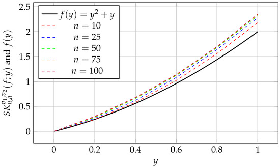
$$\begin{array}{c}f\left(t\right)=t^2+t,{\mathfrak{T}}_{n+p}={\xi }_{n+p}=n=\{10,20,40,80,160\}\\ a=10,v_1=2,v_2=4,\zeta =0.4\end{array}$$

As the value of n increases, the modified Szász–Charlier operator $S{K}_{n,a}^{v_1,v_2}(f;y)$ provides an increasingly accurate approximation of $f\left(y\right)=y^2+y$ across the interval $y\in [0,1]$.

6. Conclusions

In this work, we have introduced a new generalization of a fractional integral-type Szász–Kantorovich–Stancu operator connecting via Charlier polynomials. Several fundamental properties of the operators have been studied, including estimates for test functions and central moments. We have examined their convergence behavior and derived results for the rate of approximation. Furthermore, the order of approximation has been analyzed using the higher-order modulus of smoothness, supported by moment calculations. Convergence results concerning Peetre’s K-functional, Lipschitz-type functions have also been established. Finally, we derived results related to Korovkin’s theorem, Voronovskaya-type approximation, and Grüss–Voronovskaya-type theorems, thereby demonstrating the effectiveness and applicability of the proposed operators.

References

1. Bernstein, S.N. Démonstration du théoréme de Weierstrass fondée sur le calcul des probabilités. Commun. Kharkov Math. Soc. 1912, 13, 1–2. [Google Scholar]
2. Szász, O. Generalization of Bernstein’s polynomials to the infinite interval. J. Res. Nat. Bur. Stds. 1950, 45, 239–245. [Google Scholar] [CrossRef]
3. Özger, F.; Ersoy, M.T.; Özger, O.Z. Existence of solutions: Investigating Fredholm integral equations via a fixed-point theorem. Axioms 2024, 13, 261. [Google Scholar]
4. Özger, F.; Aslan, R.; Ersoy, M. Some Approximation Results on a Class of Szász-Mirakjan-Kantorovich Operators Including Non-negative parameter α. Numer. Funct. Anal. Optim. 2025, 46, 461–484. [Google Scholar]
5. Ayman-Mursaleen, M.; Nasiruzzaman, M.; Rao, N.; Dilshad, M.; Nisar, K.S. Approximation by the modified λ-Bernstein-polynomial in terms of basis function. AIMS Math. 2024, 9, 4409–4426. [Google Scholar] [CrossRef]
6. Ayman-Mursaleen, M. Quadratic function preserving wavelet type Baskakov operators for enhanced function approximation. Comput. Appl. Math. 2025, 44, 395. [Google Scholar] [CrossRef]
7. Braha, N.L.; Loku, V.; Mansour, T.; Mursaleen, M. A new weighted statistical convergence and some associated approximation theorems. Math. Meth. Appl. Sci. 2022, 45, 5682–5698. [Google Scholar] [CrossRef]
8. Ansari, K.J.; Mursaleen, M.; Al-Abeid, A.H. Approximation by Chlodowsky variant of Szász operators involving Sheffer polynomials. Adv. Oper. Theory 2019, 4, 321–341. [Google Scholar] [CrossRef]
9. Ansari, K.J.; Usta, F. On a modified Bernstein operators approximation method for computational solution of Volterra integral equation. J. Inequalities Appl. 2025, 2025, 8. [Google Scholar] [CrossRef]
10. Khan, A.; Mansoori, M.; Khan, K.; Mursaleen, M. Phillips-type q-Bernstein operators on triangles. J. Funct. Spaces 2021, 2021, 6637893. [Google Scholar] [CrossRef]
11. Acar, T.; Acu, A.M.; Manav, N. Approximation of functions by genuine Bernstein-Durrmeyer type operators. J. Math. Inequalities 2018, 12, 975–987. [Google Scholar] [CrossRef]
12. Acar, T.; Acu, A.M.; Muraru, C.V.; Radu, V.A. Some approximation properties by a class of bivariate operators. Math. Methods Appl. Sci. 2019, 42, 5551–5565. [Google Scholar] [CrossRef]
13. Aslan, R. Rate of approximation of blending type modified univariate and bivariate λ-Schurer-Kantorovich operators. Kuwait J. Sci. 2024, 51, 100168. [Google Scholar] [CrossRef]
14. Mohiuddine, S.A.; Singh, K.K.; Alotaibi, A. On the order of approximation by modified summation-integral-type operators based on two parameters. Demo. Math. 2023, 56, 20220182. [Google Scholar] [CrossRef]
15. Mohiuddine, S.A.; Özger, Z.O.; Özger, F.; Alotaibi, A. Construction of a new family of modified Bernstein-Schurer operators of different order for better approximation. J. Nonlinear Convex Anal. 2024, 25, 2059–2082. [Google Scholar]
16. Mursaleen, M.; Ansari, K.J.; Khan, A. Approximation properties and error estimation of q-Bernstein shifted operators. Numer. Algorithms 2020, 84, 207–227. [Google Scholar] [CrossRef]
17. Mursaleen, M.; Tabassum, S.; Fatma, R. On q-statistical summability method and its properties. Iran. J. Sci. Technol. Trans. 2022, 46, 455–460. [Google Scholar] [CrossRef]
18. Malik, G.; Khan, T.; Mursaleen, M. Approximation properties and q-statistical convergence of Kantorovich variant of Stancu type Lupaş operators. Filomat 2023, 37, 10107–10124. [Google Scholar] [CrossRef]
19. Nasiruzzaman, M.; Srivastava, H.M.; Mohiuddine, S.A. Approximation process based on parametric generalization of Schurer–Kantorovich operators and their bivariate form. Proc. Nat. Acad. Sci. India Sect. 2023, 93, 31–41. [Google Scholar] [CrossRef]
20. Nasiruzzaman, M.; Mohammed, A.O.; Serra-Capizzano, T.S.; Rao, N.; Mursaleen, M.A. Approximation results for Beta Jakimovski-Leviatan type operators via q-analogue. Filomat 2023, 37, 8389–8404. [Google Scholar] [CrossRef]
21. Rao, N.; Farid, M.; Ali, R. A Study of Szász–Durremeyer-Type Operators Involving Adjoint Bernoulli Polynomials. Mathematics 2024, 12, 3645. [Google Scholar] [CrossRef]
22. Rao, N.; Farid, M.; Jha, N.K. Szász-integral operators linking general-Appell polynomials and approximation. AIMS Math. 2025, 10, 13836–13854. [Google Scholar] [CrossRef]
23. Alamer, A.; Nasiruzzaman, M. Approximation by Stancu variant of λ-Bernstein shifted knots operators associated by bézier basis function. J. King Saud Univ. Comput. Inf. Sci. 2024, 36, 103333. [Google Scholar] [CrossRef]
24. Cai, Q.B.; Khan, A.; Mansoori, M.S.; Iliyas, M.; Khan, K. Approximation by λ-Bernstein type operators on triangular domain. Filomat 2023, 37, 1941–1958. [Google Scholar] [CrossRef]
25. Cai, Q.B.; Aslan, R.; Özger, F.; Srivastava, H.M. Approximation by a new Stancu variant of generalized (λ, μ)-Bernstein operators. Alex. Eng. J. 2024, 107, 205–214. [Google Scholar] [CrossRef]
26. Aslan, R. Some approximation properties of Riemann-Liouville type fractional Bernstein-Stancu-Kantorovich operators with order of α. Iran. J. Sci. 2025, 49, 481–494. [Google Scholar] [CrossRef]
27. Braha, N.L.; Mansour, T.; Mursaleen, M.; Acar, T. Convergence of-Bernstein operators via power series summability method. J. Appl. Math. Comput. 2021, 65, 125–146. [Google Scholar] [CrossRef]
28. Berwal, S.; Mohiuddine, S.A.; Kajla, A.; Alotaibi, A. Approximation by Riemann–Liouville type fractional α-Bernstein–Kantorovich operators. Math. Methods Appl. Sci. 2024, 47, 8275–8288. [Google Scholar] [CrossRef]
29. Baxhaku, B.; Agrawal, P.N.; Bajpeyi, S. Riemann–Liouville Fractional Integral Type Deep Neural Network Kantorovich Operators. Iran. J. Sci. 2024, 49, 711–724. [Google Scholar] [CrossRef]
30. Kajla, A.; Agrawal, P.N. Szász-Kantorovich type operators based on Charlier polynomials. Kyungpook Math. J. 2016, 56, 877–897. [Google Scholar] [CrossRef]
31. Ansari, K.J.; Sharma, V.; Samei, M.E. Charlier polynomial-based modified Kantorovich-Szász type operators and related approximation outcomes. J. Anal. 2024, 32, 3315–3333. [Google Scholar] [CrossRef]
32. Varma, S.; Taşdelen, F. Szász type operators involving Charlier polynomials. Math. Comput. Model. 2012, 56, 118–122. [Google Scholar] [CrossRef]
33. Ansari, K.J.; Mursaleen, M.; Shareef, K.M.; Ghouse, M. Approximation by modified Kantorovich–Szász type operators involving Charlier polynomials. Adv. Differ. Equ. 2020, 2020, 192. [Google Scholar] [CrossRef]
34. Korovkin, P. On convergence of linear positive operators in the space of continuous functions (russian). Dokl. Akad. Nauk. SSSR (NS) 1953, 90, 961. [Google Scholar]
35. Ditzian, Z.; Totik, V. K-functional and weighted moduli of smoothness. J. Approx. Theory 1990, 63, 3–29. [Google Scholar] [CrossRef][Green Version]
36. Ditzian, Z.; Totik, V. Moduli of Smoothness; Springer Science & Business Media: Berlin/Heidelberg, Germany, 2012; Volume 9. [Google Scholar][Green Version]
37. Özarslan, M.A.; Aktuğlu, H. Local approximation for certain King type operators. Filomat 2013, 27, 173–181. [Google Scholar] [CrossRef]
38. Gonska, H.; Rasa, I. A Voronovskaya estimate with second order modulus of smoothness. Proc. Math. Inequal. 2008.
39. Gonska, H.H. Degree of approximation by Lacunary interpolators:(0,⋯,r−2,r) interpolation. Rocky Mt. J. Math. 1989, 19, 157–171. [Google Scholar] [CrossRef]
Figure 1. Convergence analysis of operator S K n + p , a v 1 , v 2 ( f ; y ) .
Mathematics 13 03039 g001
Disclaimer/Publisher’s Note: The statements, opinions and data contained in all publications are solely those of the individual author(s) and contributor(s) and not of MDPI and/or the editor(s). MDPI and/or the editor(s) disclaim responsibility for any injury to people or property resulting from any ideas, methods, instructions or products referred to in the content.