Q-Function-Based Diagnostic and Spatial Dependence in Reparametrized t-Student Linear Model

Abstract

Characterizingthe spatial variability of agricultural data is a fundamental step in precision agriculture, especially in soil management and the creation of differentiated management units for increasing productivity. Modeling the spatial dependence structure using geostatistical methods is of great importance for efficiency, estimating the parameters that define this structure, and performing kriging-based interpolation. This work presents diagnostic techniques for global and local influence and generalized leverage using the displacement of the conditional expectation of the logarithm of the joint-likelihood, called the Q-function. This method is used to identify the presence of influential observations that can interfere with parameter estimations, geostatistics model selection, map construction, and spatial variability. To study spatially correlated data, we used reparameterized t-Student distribution linear spatial modeling. This distribution has been used as an alternative to the normal distribution when data have outliers, and it has the same form of covariance matrix as the normal distribution, which enables a direct comparison between them. The methodology is illustrated using one real data set, and the results showed that the modeling was more robust in the presence of influential observations. The study of these observations is indispensable for decision-making in precision agriculture.

1. Introduction

Geostatistics differs from classical statistics because the models of classical statistics usually focus on frequency checking and incorporate the interpretation of the spatial correlation of the samples. It assumes that the difference between two sample points depends on the distance between them and the orientation of the points, that is, closer pairs of observations are more similar to each other than pairs of more distant observations. However, in practice, atypical observations can affect the behavior of spatial dependence, especially when the normal distribution is assumed. Several authors, such as [1,2,3,4] have presented more robust approaches, with model estimates that are less sensitive to these observations. An alternative proposal by [5], studied later by [6], is to use the reparametrized t-Student distribution, which belongs to the symmetric distribution class and enables us to reduce the influence of outliers, as well as allowing for the existence of the second finite moment and a direct comparison between the matrix t-Student and the normal distribution. According to [7], it is possible that a single observation has a significant influence on the results of an analysis of spatial data, being able to considerably alter the results that define the spatial dependence structure, consequently changing the construction of the maps.

Following this thinking, diagnostic analysis is extremely important for detecting these observations. Several diagnostic analyses are presented as follows: Ref. [8] assessed local influence using elliptical linear models with a longitudinal structure; Ref. [9] used diagnostic techniques to assess the sensitivity of maximum likelihood estimators, the covariance function, and the linear predictor to small perturbations in the data and the assumptions of the spatial linear model. Refs. [10,11] worked with diagnostic techniques in Gaussian spatial linear models with repetition. Ref. [12] worked with the diagnostics of influence in spatial models with censored responses.

The purpose of this paper is to extend the work of [6] for the application of diagnostic analysis in the reparametrized t-Student distribution, through global and local influence techniques developed using the maximum likelihood and Q-function, which is an alternative to Cook’s procedure [13].

This paper proceeds as follows. The Section 2 is divided into subsections as follows: The t-Student spatial linear model subsection presents the reparametrized t-Student linear spatial model. The maximum likelihood estimation subsection presents the maximum likelihood estimation and the development of the parameter estimation process. The iterative algorithm subsection describes the algorithm. The asymptotic standard error estimation subsection explains how to obtain an estimate of the asymptotic standard errors. The selection of the parameter of form $\eta$ subsection describes the criteria for selecting the parameter of the form $\eta$. The QQ-plot subsection describes the methodology for obtaining the QQ-plot graph. The influence diagnostics subsection presents the development of diagnostic tools to detect influential points using techniques of global and local influence and generalized leverage. The Section 3 presents the application of the methodology to a real data set and illustrates the method for analyzing real data for the reparameterized t-Student model, presenting the results obtained. The Section 4 presents a brief discussion of the results compared to the works found in the literature. The Section 5 presents the conclusions of the work.

2. Materials and Methods

2.1. The t-Student Spatial Linear Model

An alternative to the multivariate normal distribution is the multivariate t-Student distribution; this distribution has been widely used in the study of real data because it has heavier tails and allows for the incorporation of the atypical points present in the data set. Furthermore, it is a symmetrical distribution with an additional parameter, the degree of freedom, which is represented by v ($v>0$) and allows us to model the kurtosis of the data.

Ref. [5] suggests reparameterizing the t-Student distribution to allow for a direct comparison between the estimation of the mean vector parameters and the covariance matrix with the normal model. The reparameterization of this distribution is a transformation of the degrees of freedom, considering $\eta =1/v$. This reparameterization is justified by the importance of modeling the spatial dependence structure, since the new shape parameter ($\eta$) is bounded ($0<\eta <1/2$) due to the assumption of the process having a finite second moment. This allows estimation of the model parameters using the EM algorithm, which is used in Kriging interpolation and later in map construction [14].

Following the methodology of [6], which presents the reparametrized multivariate t-Student distribution, the transformation $v=1/\eta$ is applied. It considers that $\mathbf{Y}={(Y_1,\dots ,Y_n)}^{\top }$, where a random vector follows a reparametrized t-Student distribution with a parameter of form $\eta$ fixed, where $0<\eta <{\displaystyle \frac{1}{2}}$, with covariance matrix $\mathbf{\Sigma }$, $n\times n$, and mean vector $E\left(\mathbf{Y}\right)=\mathit{\mu }$. Its probability density function is given in Equation (1) as follows:

$$f_{\mathit{Y}}\left(y\right)=K_n\left(\eta \right){\left|\mathbf{\Sigma }\right|}^{-{\displaystyle \frac{1}{2}}}{\left[1+c\left(\eta \right)\delta \right]}^{-{\displaystyle \frac{1}{2\eta }}(1+n\eta )},$$

(1)

where

$$K_n\left(\eta \right)={\left({\displaystyle \frac{c\left(\eta \right)}{\pi }}\right)}^{{\displaystyle \frac{n}{2}}}{\displaystyle \frac{\Gamma \left(\frac{1+n\eta }{2\eta }\right)}{\Gamma \left(\frac{1}{2\eta }\right)}},$$

with $\delta ={\left(\mathit{Y}-\mu \right)}^T{\mathbf{\Sigma }}^{-1}\left(\mathit{Y}-\mu \right)$ is the Mahalanobis distance, $c\left(\eta \right)=\eta /(1-2\eta )$ for $0<\eta <{\displaystyle \frac{1}{2}}$. Let $\mathit{Y}\sim T_n(\mathit{\mu },\mathbf{\Sigma },\eta )$ denote a random vector following an n-multivariate reparameterized t-Student distribution. The stochastic representation of $\mathit{Y}$ is given by

$$\mathit{Y}\stackrel{d}{=}\mu +V^{-1/2}\mathit{Z},$$

where $\mathit{Z}\sim N_n\left(\mathbf{0},\mathbf{\Sigma }\right)$, $V\sim Gamma\left({\displaystyle \frac{1}{2\eta }},{\displaystyle \frac{1}{2c\left(\eta \right)}}\right)$, $c\left(\eta \right)=\eta /(1-2\eta )$, $0<\eta <{\displaystyle \frac{1}{2}}$; V add $\mathit{Z}$ independent.

To study spatial dependence, consider an isotropic second-order stochastic process $\left\{\mathit{Y}\left({\mathbf{s}}_i\right),{\mathbf{s}}_i\in \mathit{S}\right\}$, where $\mathit{S}\subset {\mathfrak{R}}^2$ and ${\mathfrak{R}}^2$ is a bi-dimensional Euclidean space. Let $\mathbf{Y}={(Y\left({\mathbf{s}}_1\right),\dots ,Y\left({\mathbf{s}}_n\right))}^{\top }$ be an $n\times 1$ response vector corresponding to the sites ${\mathbf{s}}_i$ with $i=1,\dots ,n$, following an n-multivariate reparameterized t-Student distribution, denoted by $\mathit{Y}\sim T_n(\mathit{\mu },\mathbf{\Sigma },\eta )$, where each element $Y\left({\mathbf{s}}_i\right)$ can be written as $Y\left({\mathbf{s}}_i\right)=\mu \left({\mathbf{s}}_i\right)+e\left({\mathbf{s}}_i\right)$, $i=1,\dots ,n$, where both the deterministic term $\mu \left({\mathbf{s}}_i\right)$ and stochastic $e\left({\mathbf{s}}_i\right)$ may depend on the spatial location at which $Y\left({\mathbf{s}}_i\right)$ is observed. It is assumed that random errors $e\left({\mathbf{s}}_i\right)$ have an expectation equal to zero, that is, $E\left[e\left({\mathbf{s}}_i\right)\right]=0$, and the variation between points is determined by some covariance function $Cov\left[e\left({\mathbf{s}}_i\right),e\left({\mathbf{s}}_u\right)\right]=Cov\left[Y\left({\mathbf{s}}_i\right),Y\left({\mathbf{s}}_u\right)\right]=C\left({\mathbf{s}}_i,{\mathbf{s}}_u\right)={\sigma }_{iu}$, for $i,u=1,\dots ,n$. Suppose that for some known function of ${\mathbf{s}}_i$, $x_1\left({\mathbf{s}}_i\right),\dots ,x_p\left({\mathbf{s}}_i\right)$, the mean of the stochastic process is given in Equation (2) as follows:

$$\mathit{\mu }\left({\mathbf{s}}_i\right)=\sum _{i=1}^p{x}_j\left({\mathbf{s}}_i\right){\beta }_j,$$

(2)

where ${\beta }_1,\dots ,{\beta }_p$ are unknown parameters for estimation.

In matrix notation, the spatial linear model is given by

$$\mathit{Y}=\mathit{X}\mathit{\beta }+\mathit{\epsilon },$$

(3)

where $\mathit{Y}\sim T_n(\mathit{X}\mathit{\beta },\mathbf{\Sigma },\eta )$, $\mathit{X}$ is an $n\times p$ full rank matrix, with i-th row an $n\times p$ vector ${\mathit{x}}_{\mathit{i}}^{\top }=(x_{i1},\dots ,x_{ip})$ with explanatory variables at the site ${\mathbf{s}}_i$, $\mathit{\beta }={\left({\beta }_1,\dots ,{\beta }_p\right)}^{\top }$ is a $p\times 1$ vector of unknown parameters to estimate and $\mathit{\epsilon }={\left(e\left({\mathbf{s}}_1\right),\dots ,e\left({\mathbf{s}}_n\right)\right)}^{\top }$ are components correlated with variance with $\mathit{\epsilon }\sim T_n(\mathbf{0},\mathbf{\Sigma },\eta )$.

The spatial modeling given in Equation (3) depends on the structure of the covariance matrix $\mathbf{\Sigma }=\left[\left({\sigma }_{iu}\right)\right]$, where ${\sigma }_{iu}=C({\mathbf{s}}_i,{\mathbf{s}}_u)$ for $i,u=1,\dots ,n$ of the stochastic process $\mathit{Y}$. A covariance function $C({\mathbf{s}}_i,{\mathbf{s}}_u)$ is used in the spatial dependence study of the stationary process and is specified by a three-dimensional vector $\mathit{\tau }={({\tau }_1,{\tau }_2,{\tau }_3)}^{\top }$. As presented by [15], the parametric form is given in Equation (4) as follows:

$$\mathbf{\Sigma }={\tau }_1{\mathit{I}}_{\mathit{n}}+{\tau }_2\mathit{R}\left({\tau }_3\right),$$

(4)

where ${\tau }_1$ is the nugget effect, ${\tau }_1\ge 0$; ${\tau }_2$ is known as sill, ${\tau }_2\ge 0$; ${\mathit{I}}_{\mathit{n}}$ is an identity matrix of order n; $\mathit{R}\left({\tau }_3\right)$ is an $n\times n$ symmetric matrix, where the elements are functions of ${\tau }_3>0$, $\mathit{R}=\mathit{R}\left({\tau }_3\right)=\left[\left(r_{ij}\right)\right]$, where $r_{ii}=1$, and $r_{ij}={\tau }_2^{-1}C({\mathbf{s}}_i,{\mathbf{s}}_j)$ for ${\tau }_2\ne 0$, and $r_{ij}=0$ for ${\tau }_2=0$, $i\ne j=1,\dots ,n$, where $r_{ij}$ depends on the Euclidean distance, $h_{ij}=\parallel {\mathbf{s}}_i-{\mathbf{s}}_j\parallel$, between points ${\mathbf{s}}_i$ and ${\mathbf{s}}_j$. An alternative reparametrization of the covariance function $C\left({\mathbf{s}}_i,{\mathbf{s}}_u\right)=C\left(h_{iu}\right)$ is suggested by [16] and adapted by [6], assisting in the identifiability of the model. In this paper, we considered the parameters ${\varphi }_1={\tau }_1$, ${\varphi }_2={\tau }_2/{\tau }_3^{2\kappa }$ and ${\varphi }_3={\tau }_3$. This last parameter was considered fixed, and reparametrization of $C\left(h_{iu}\right)$ was based on the same criteria established by [6].

2.2. Maximum Likelihood Estimation

Under the assumption that $\mathit{Y}\sim T_n(\mathit{X}\mathit{\beta },\mathbf{\Sigma },\eta )$, where $\eta$ is the fixed form parameter and $\theta ={\left({\mathit{\beta }}^{\top },{\mathit{\varphi }}^{\top }\right)}^{\top }$, with $\mathit{\beta }={\left({\beta }_1,\dots ,{\beta }_p\right)}^{\top }$ and $\mathit{\varphi }={\left({\varphi }_1,{\varphi }_2\right)}^{\top }$ with ${\varphi }_1$ and ${\varphi }_2$ as unknown parameters and ${\varphi }_3$ as a parameter to be defined and fixed according to the semivariogram, the log-likelihood of the reparameterized t-Student distribution is given in Equation (5) by:

$$\mathcal{L}\left(\mathit{\theta }\right)=log{K}_n\left(\eta \right)-{\displaystyle \frac{1}{2}}log\left|\mathbf{\Sigma }\right|-{\displaystyle \frac{1}{2\eta }}\left(1+n\eta \right)log\left(1+c\left(\eta \right)\delta \right),$$

(5)

where

• $log{K}_n\left(\eta \right)={\displaystyle \frac{n}{2}}log\left({\displaystyle \frac{c\left(\eta \right)}{\pi }}\right)+log\Gamma \left({\displaystyle \frac{1+n\eta }{2\eta }}\right)-log\Gamma \left({\displaystyle \frac{1}{2\eta }}\right)$,
• $\delta ={\left(\mathit{Y}-\mathit{X}\mathit{\beta }\right)}^{\top }{\mathbf{\Sigma }}^{-1}\left(\mathit{Y}-\mathit{X}\mathit{\beta }\right)$, $c\left(\eta \right)=\eta /\left(1-2\eta \right)$, $0<\eta <{\displaystyle \frac{1}{2}}$.

The scores function can be written as:

• $\mathit{U}\left(\mathit{\beta }\right)={\displaystyle \frac{\mathit{\partial }\mathcal{L}\left(\mathit{\theta }\right)}{\partial \beta }}=w\left(\delta \right){\mathit{X}}^{\top }{\mathbf{\Sigma }}^{-1}\mathit{\epsilon }$,
• $\mathit{U}\left(\mathit{\varphi }\right)={\displaystyle \frac{\mathit{\partial }\mathcal{L}\left(\mathit{\theta }\right)}{\partial {\varphi }_j}}=-{\displaystyle \frac{1}{2}}[tr\left({\mathbf{\Sigma }}^{-1}{\dot{\mathbf{\Sigma }}}_j\right)-w\left(\delta \right){\mathit{\epsilon }}^{\top }{\mathbf{\Sigma }}^{-1}{\dot{\mathbf{\Sigma }}}_j{\mathbf{\Sigma }}^{-1}\mathit{\epsilon }]$,
• where ${\dot{\mathbf{\Sigma }}}_j=\partial \mathbf{\Sigma }/\partial {\varphi }_j$ for $j=1,2$, $w\left(\delta \right)=((1+n\eta )/\eta )c\left(\eta \right)q^{-1}$, $q=\left(1+c\left(\eta \right)\delta \right)$ and $\mathit{\epsilon }=\left(\mathit{Y}-\mathit{X}\mathit{\beta }\right)$.

The vector of parameters $\theta ={\left({\mathit{\beta }}^{\top },{\mathit{\varphi }}^{\top }\right)}^{\top }$ can be estimated by maximum likelihood (ML) from the solution of the score functions $\mathit{U}\left(\mathit{\beta }\right)=\mathbf{0}$ and $\mathit{U}\left(\mathit{\varphi }\right)=\mathbf{0}$.

For the parameter $\widehat{\mathit{\beta }}$ estimated by the maximum likelihood, the solution of the function is obtained immediately as follows:

$$\begin{array}{c}\hfill \widehat{\mathit{\beta }}={\left({\mathit{X}}^{\top }{\left({\mathbf{\Sigma }}^{\left(k\right)}\right)}^{-1}\mathit{X}\right)}^{-1}\left({\mathit{X}}^{\top }{\left({\mathbf{\Sigma }}^{\left(k\right)}\right)}^{-1}\mathit{Y}\right),\end{array}$$

with k representing the k-th iteration.

To obtain the parameter $\widehat{\mathit{\varphi }}$ estimated by maximum likelihood, ${\varphi }_j$ with $j=1,2$ is determined through the system resolution (6). From $\mathit{U}\left(\mathit{\varphi }\right)=\mathbf{0}$ we have:

$$\begin{array}{c}\hfill tr\left({\mathbf{\Sigma }}^{-1}{\dot{\mathbf{\Sigma }}}_j\right)=tr\left({\mathbf{\Sigma }}^{-1}{\dot{\mathbf{\Sigma }}}_j{\mathbf{\Sigma }}^{-1}\mathit{E}\right),\end{array}$$

(6)

where $\mathit{E}=w\left(\delta \right)\mathit{\epsilon }{\mathit{\epsilon }}^{\top }$.

Considering $\mathbf{\Sigma }={\displaystyle \sum _{l=1}^2}{\varphi }_l{\dot{\mathbf{\Sigma }}}_l$, where ${\dot{\mathbf{\Sigma }}}_1={\mathit{I}}_n$ and ${\dot{\mathbf{\Sigma }}}_2=\mathit{R}\left({\varphi }_3\right)$, (6) is applied:

$$\begin{array}{c}\hfill \sum _{l=1}^{2}tr\left({\mathbf{\Sigma }}^{-1}{\dot{\mathbf{\Sigma }}}_j{\mathbf{\Sigma }}^{-1}{\dot{\mathbf{\Sigma }}}_l\right){\varphi }_l=tr\left({\mathbf{\Sigma }}^{-1}{\dot{\mathbf{\Sigma }}}_j{\mathbf{\Sigma }}^{-1}\mathit{E}\right).\end{array}$$

(7)

Notice that in matrix notation, the system (7) can be written as:

$$\begin{array}{c}\hfill \mathit{A}·\mathit{\varphi }=\mathit{b},\end{array}$$

where the matrix $\mathit{A}$ of order $2\times 2$, with elements $a_{jl}=tr\left({\mathbf{\Sigma }}^{-1}{\dot{\mathbf{\Sigma }}}_j{\mathbf{\Sigma }}^{-1}{\dot{\mathbf{\Sigma }}}_l\right)$ and $\mathit{b}$ a vector of order $(2\times 1)$, with elements $b_j=tr\left({\mathbf{\Sigma }}^{-1}{\dot{\mathbf{\Sigma }}}_j{\mathbf{\Sigma }}^{-1}\mathit{E}\right)$, which correspond to $a_{11}=tr\left({\mathbf{\Sigma }}^{-1}{\mathbf{\Sigma }}^{-1}\right)$, $a_{12}=a_{21}=tr\left({\mathbf{\Sigma }}^{-1}{\mathbf{\Sigma }}^{-1}\mathit{R}\left({\varphi }_3\right)\right)$, $a_{22}=tr\left({\mathbf{\Sigma }}^{-1}\mathit{R}\left({\varphi }_3\right){\mathbf{\Sigma }}^{-1}\mathit{R}\left({\varphi }_3\right)\right)$, $b_1=tr\left({\mathbf{\Sigma }}^{-1}{\mathbf{\Sigma }}^{-1}\mathit{E}\right)$ and $b_2=tr\left({\mathbf{\Sigma }}^{-1}\mathit{R}\left({\varphi }_3\right){\mathbf{\Sigma }}^{-1}\mathit{E}\right)$. The estimation process is given in Equation (8) by the system resolution:

$$\begin{array}{c}\hfill \widehat{\mathit{\varphi }}={\mathit{A}}^{-1}·\mathit{b}.\end{array}$$

(8)

The iterative algorithm section describes the algorithm for obtaining the estimation of the parameters of $\mathit{\theta }$ through iteration; in other words, it will obtain $\widehat{\mathit{\theta }}={\mathit{\theta }}^{\left(k\right)}$ when it reaches the convergence criterion in the k-th iteration.

2.3. Iterative Algorithm

Based on [17], to obtain the parameter estimation of $\mathit{\theta }$, we must use an iterative algorithm and the following procedures:

Initial Iteration: Set $k=0$, where k represents the iteration phase:

• $1^{\underline{\mathrm{o}}}$ step: Define an initial shot to the parameter to be estimated ${\mathit{\theta }}^{\left(k\right)}={\mathit{\theta }}^0$, in what ${\mathit{\theta }}^0={({\mathit{\beta }}^0,{\mathit{\varphi }}^0,{\eta }^0)}^{\top }$. In this study, we choose to define the initial parameters ${\mathit{\beta }}^0$ and ${\mathit{\varphi }}^0$, obtaining them in a regression model with a normal distribution, and ${\eta }^0$ is fixed and defined for all iterations, which will later be chosen by the cross-Validation criterion ($CV$) and Trace ($T_r$) presented in the selection of the parameter of form $\eta$ section.
• $2^{\underline{\mathrm{o}}}$ step: We calculate the following Equations from the initial parameters obtained from the $1^{\underline{\mathrm{o}}}$ step:
  ${\mathbf{\Sigma }}^{\left(k\right)}={\varphi }_1^{\left(k\right)}\mathit{I}+{\varphi }_2^{\left(k\right)}{\mathit{R}}^{\left(k\right)}\left({\varphi }_3\right)$, in which ${\varphi }_3$ is fixed on the initial shot.
  $c\left(\eta \right)={\displaystyle \frac{\eta }{1-2\eta }}$,
  $q^{\left(k\right)}=(1+c\left(\eta \right){\delta }^{\left(k\right)})$,
  ${\delta }^{\left(k\right)}={\left({\mathit{\epsilon }}^{\left(k\right)}\right)}^{\top }{\left({\mathbf{\Sigma }}^{\left(k\right)}\right)}^{-1}{\mathit{\epsilon }}^{\left(k\right)}$,
  ${\mathit{\epsilon }}^{\left(k\right)}=(\mathit{Y}-\mathit{X}{\mathit{\beta }}^{\left(k\right)})$,
  $w{\left(\delta \right)}^{\left(k\right)}=\left({\displaystyle \frac{1+n\eta }{\eta }}\right)c\left(\eta \right){\left(q^{\left(k\right)}\right)}^{-1}$,
  ${\mathit{\beta }}^{\left(k\right)}={\left({\mathit{X}}^{\top }{\left({\mathbf{\Sigma }}^{\left(k\right)}\right)}^{-1}\mathit{X}\right)}^{-1}\left({\mathit{X}}^{\top }{\left({\mathbf{\Sigma }}^{\left(k\right)}\right)}^{-1}\mathit{Y}\right)$,
  ${\mathit{E}}^{\left(k\right)}=w{\left(\delta \right)}^{\left(k\right)}{\mathit{\epsilon }}^{\left(k\right)}{\left({\mathit{\epsilon }}^{\left(k\right)}\right)}^{\top },$
  where $\mathit{R}=\mathit{R}\left({\varphi }_3\right)$ is the covariance function that depends on the exponential, Gaussian, or Matérn family models, where $\mathit{R}$ is introduced by [9]. Verify that these equations calculated in the $2^{\underline{\mathrm{o}}}$ step are being considered as initials where $k=0$.
• $3^{\underline{\mathrm{o}}}$ step: from this moment, we will update the parameters to $(k+1)$ where ${\mathit{\theta }}^{(k+1)}={({\mathit{\beta }}^{(k+1)},{\mathit{\varphi }}^{(k+1)},{\eta }^0)}^{\top }$. Consider the following procedures:
• ${3.1}^{\underline{\mathrm{o}}}$ step: Updating the linear parameters ${\varphi }_1$ and ${\varphi }_2$ of $\mathbf{\Sigma }$, through the linear system (9):

  $$\begin{array}{c}\hfill {\mathit{A}}^{\left(k\right)}·{\mathit{\varphi }}^{(k+1)}={\mathit{b}}^{\left(k\right)},\end{array}$$

  (9)

  where the matrix ${\mathit{A}}^{\left(k\right)}$ of order $2\times 2$, with elements $a_{jl}^{\left(k\right)}=tr\left({\left({\mathbf{\Sigma }}^{\left(k\right)}\right)}^{-1}{\dot{\mathbf{\Sigma }}}_j{\left({\mathbf{\Sigma }}^{\left(k\right)}\right)}^{-1}{\dot{\mathbf{\Sigma }}}_l\right)$ and ${\mathit{b}}^{\left(k\right)}$ a vector of order $2\times 1$ with elements $b_j^{\left(k\right)}=tr\left({\left({\mathbf{\Sigma }}^{\left(k\right)}\right)}^{-1}{\dot{\mathbf{\Sigma }}}_j{\left({\mathbf{\Sigma }}^{\left(k\right)}\right)}^{-1}{\mathit{E}}^{\left(k\right)}\right)$, where $j,l=1,2$ correspond to $a_{11}^{\left(k\right)}=tr\left({\left({\mathbf{\Sigma }}^{\left(k\right)}\right)}^{-1}{\left({\mathbf{\Sigma }}^{\left(k\right)}\right)}^{-1}\right)$, $a_{12}^{\left(k\right)}=a_{21}^{\left(k\right)}=tr\left({\left({\mathbf{\Sigma }}^{\left(k\right)}\right)}^{-1}{\left({\mathbf{\Sigma }}^{\left(k\right)}\right)}^{-1}{\mathit{R}}^{\left(k\right)}\left({\varphi }_3\right)\right)$, $a_{22}^{\left(k\right)}=tr\left({\left({\mathbf{\Sigma }}^{\left(k\right)}\right)}^{-1}{\mathit{R}}^{\left(k\right)}\left({\varphi }_3\right){\left({\mathbf{\Sigma }}^{\left(k\right)}\right)}^{-1}{\mathit{R}}^{\left(k\right)}\left({\varphi }_3\right)\right)$, to the vector $b_1^{\left(k\right)}=tr\left({\left({\mathbf{\Sigma }}^{\left(k\right)}\right)}^{-1}{\left({\mathbf{\Sigma }}^{\left(k\right)}\right)}^{-1}{\mathit{E}}^{\left(k\right)}\right)$ and $b_2^{\left(k\right)}=tr\left({\left({\mathbf{\Sigma }}^{\left(k\right)}\right)}^{-1}{\mathit{R}}^{\left(k\right)}\left({\varphi }_3\right){\left({\mathbf{\Sigma }}^{\left(k\right)}\right)}^{-1}{\mathit{E}}^{\left(k\right)}\right)$.
• ${3.2}^{\underline{\mathrm{o}}}$ step: Getting ${\mathit{\varphi }}^{(k+1)}$ from the steps $\left({3.1}^{\underline{\mathrm{o}}}\right)$, we update ${\mathbf{\Sigma }}^{(k+1)}$, which will be used to update the parameter ${\mathit{\beta }}^{(k+1)}$, by the expression given in Equation (10) by:

  $$\begin{array}{c}\hfill {\mathit{\beta }}^{(k+1)}={\left({\mathit{X}}^{\top }{\left({\mathbf{\Sigma }}^{(k+1)}\right)}^{-1}\mathit{X}\right)}^{-1}\left({\mathit{X}}^{\top }{\left({\mathbf{\Sigma }}^{(k+1)}\right)}^{-1}\mathit{Y}\right).\end{array}$$

  (10)
• $4^{\underline{\mathrm{o}}}$ step: the iteration ends, defining ${\mathit{\theta }}^{(k+1)}={\mathit{\theta }}^{\left(1\right)}$, obtained by updating step $\left({3.1}^{\underline{\mathrm{o}}}\right)$ and step $\left({3.2}^{\underline{\mathrm{o}}}\right)$. From ${\mathit{\theta }}^{\left(1\right)}$ apply the convergence criterion that is defined for this algorithm: if $\left|\right|{\mathit{\theta }}^{(k+1)}-{\mathit{\theta }}^{\left(k\right)}\left|\right|<e_1$ as $\eta$ and ${\varphi }_3$ are fixed, only verify the convergence to $\left|\right|{\mathit{\beta }}^{(k+1)}-{\mathit{\beta }}^{\left(k\right)}\left|\right|<e_1$ and $\left|\right|{\mathit{\varphi }}_j^{(k+1)}-{\mathit{\varphi }}_j^{\left(k\right)}\left|\right|<e_1$ ($j=1,2$) or $|{\mathcal{L}}_c\left({\mathit{\theta }}^{(k+1)}\right)-{\mathcal{L}}_c\left({\mathit{\theta }}^{\left(k\right)}\right)|<e_2$ stop and define $\widehat{\mathit{\theta }}={\mathit{\theta }}^{(k+1)}$, otherwise $k=k+1$ return to the $2^{\underline{\mathrm{o}}}$ step. Having $e_1$ and $e_2$ constant tolerance. In general, typical tolerance values are ${10}^{-3}$ and ${10}^{-6}$, respectively.

2.4. Asymptotic Standard Error Estimation

Asymptotic standard errors can be calculated by inverting the expected information matrix, $\mathit{F}\left(\mathit{\theta }\right)$, where $\mathit{F}\left(\mathit{\theta }\right)=E\left[-\mathit{L}\left(\mathit{\theta }\right)\right]$, with $\mathit{L}\left(\mathit{\theta }\right)={\partial }^2\mathcal{L}\left(\mathit{\theta }\right)/\partial \mathit{\theta }\partial {\mathit{\theta }}^{\top }$. For the reparametrized t-Student $\mathit{F}\left(\mathit{\theta }\right)$ is given in Equation (11) by [18],

$$\begin{array}{c}\hfill \mathit{F}=\mathit{F}\left(\mathit{\theta }\right)=\left(\begin{array}{cc}{\mathit{F}}_{\mathit{\beta }\mathit{\beta }}& \mathbf{0}\\ \mathbf{0}& {\mathit{F}}_{\mathit{\varphi }\mathit{\varphi }}\end{array}\right),\end{array}$$

(11)

where

$$\begin{array}{ccc}\hfill {\mathit{F}}_{\mathit{\beta }\mathit{\beta }}={\mathit{F}}_{\mathit{\beta }\mathit{\beta }}\left(\mathit{\beta }\right)& =& {\displaystyle \frac{\left(1+n\eta \right)}{\left(1-2\eta \right)\left(1+\left(n+2\right)\eta \right)}}{\mathit{X}}^{\top }{\mathbf{\Sigma }}^{-1}\mathit{X},\hfill \end{array}$$

and

$$\begin{array}{ccc}\hfill {\mathit{F}}_{\mathit{\varphi }\mathit{\varphi }}={\mathit{F}}_{\mathit{\varphi }\mathit{\varphi }}\left(\mathit{\varphi }\right)& =& {\displaystyle \frac{1}{4}}\left({\displaystyle \frac{\partial ve{c}^T\left(\mathbf{\Sigma }\right)}{\partial \varphi }}\right)\left[2{\displaystyle \frac{\left(1+n\eta \right)}{\left(1+\left(n+2\right)\eta \right)}}\left({\mathbf{\Sigma }}^{-1}\otimes {\mathbf{\Sigma }}^{-1}\right){\mathit{N}}_n+\right.\hfill \\ \hfill & & \left.\left({\displaystyle \frac{\left(1+n\eta \right)}{\left(1+\left(n+2\right)\eta \right)}}-1\right)vec\left({\mathbf{\Sigma }}^{-1}\right)ve{c}^{\top }\left({\mathbf{\Sigma }}^{-1}\right)\right]\left({\displaystyle \frac{\partial vec\left(\mathbf{\Sigma }\right)}{\partial {\mathit{\varphi }}^{\top }}}\right),\hfill \end{array}$$

where ${\mathit{N}}_n={\displaystyle \frac{1}{2}}\left({\mathit{I}}_{n^2}+{\mathit{K}}_n\right)$, ${\mathit{K}}_n$ is the commutation matrix of order $n^2\times n^2$, and ${\mathit{I}}_{n^2}$ is the identity matrix of order $n^2\times n^2$ (see [19]).

2.5. Selection of the Parameter of Form $\eta$

According to [20,21], the log-likelihood function given in Equation (5) is decreasing in $\eta$, so the estimation of this parameter cannot be obtained through the maximization of the log-likelihood ($\mathcal{L}\left(\mathit{\theta }\right)$). As an alternative, Ref. [22] proposes using a matrix trace of the asymptotic covariance of an estimated average as a criterion in the selection of a better model for the class of elliptical distributions. Following this thought, Ref. [21] shows the trace criterion and cross-validation to select the degree of freedom v of the spatial liner t-Student model. From these propositions, Ref. [6] presents the trace criterion $\left(T_r\right)$ and the cross-validation criterion $\left(CV\right)$ to select the form parameter $\eta$ to the reparameterized t-Student spatial linear model. For both methods, the best parameter of the form $\left(\eta \right)$ is determined by the smallest cross-validation and trace values. After choosing, the model parameter Matérn $\left(\kappa \right)$ [23] is selected according to the smallest asymptotic standard error.

2.6. QQ-Plot

Following the methodology presented in [24] and the set of data $\{\mathit{Y}\left(s_1\right),\dots ,\mathit{Y}\left(s_n\right)\}$, we determine the vector of the residuals $\widehat{\mathit{\epsilon }}=(\mathit{Y}-\mathit{X}\widehat{\mathit{\beta }})$, where $\widehat{\mathit{\beta }}={\left({\mathit{X}}^{\top }{\widehat{\mathbf{\Sigma }}}^{-1}\mathit{X}\right)}^{-1}\left({\mathit{X}}^{\top }{\widehat{\mathbf{\Sigma }}}^{-1}\mathit{Y}\right)$, $\widehat{\mathit{\beta }}$ being the parameter vector and $\widehat{\mathbf{\Sigma }}$ the covariance matrix, obtained due to the iterative algorithm section and the selection of the parameter of form $\eta$. From the estimate of the covariance matrix $\widehat{\mathbf{\Sigma }}$, we use the Cholesky decomposition obtained by $\widehat{\mathbf{\Sigma }}=\widehat{\mathit{L}}{\widehat{\mathit{L}}}^{\top }$, where $\widehat{\mathit{L}}$ is the inferior triangular matrix of order n. Using the inverse matrix ${\widehat{\mathit{L}}}^{-1}$, we determine ${\widehat{\mathit{\epsilon }}}_{nc}={\widehat{\mathit{L}}}^{-1}\widehat{\mathit{\epsilon }}$, defined as the vector of uncorrelated residuals. Then we used the methodology [25] with the packages qqplotr and ggplot2 in the R program to build QQ plots, considering as sample data the vector of uncorrelated residuals ${\widehat{\mathit{\epsilon }}}_{nc}$ and as theoretical data the random vector with the distribution of the t-Students of both orders n. To obtain the confidence intervals, we utilized the [26] package with the application of the boot method, which creates confidence bands based on a parametric Bootstrap.

2.7. Influence Diagnostics

A study of great importance in the analysis of diagnosis is the influential observation detection; in other words, points exercising a disproportionate weight in the estimations of the model parameters or even in the significance of the parameters. Point detection may be the most well-known technique for evaluating the impact of the particular observation removal regression’s estimates. This paper considers two types of influence diagnostics: global and local influence.

2.8. Global Influence

Deleting cases is a common way to assess the effect of an observation on the estimation process. This is a global influence analysis, since the effect of the observation is evaluated by eliminating it from the data set.

2.8.1. Global Influence Based on the Likelihood

The global influence analysis is based on the elimination of one or more observations considered influential in the data set, and thus assesses the impact on the parameter estimates. This type of diagnostic technique is discussed by [27,28,29,30]. One of the most used measures of the changes in estimated parameters after excluding the observations is called Cook’s distance (see [31]). This measure was initially proposed for normal models and was quickly expanded to several model classes. Following the proposal of [30], the Cook’s distance, based on the ML estimator $\widehat{\mathit{\theta }}$, of $\mathit{\theta }={\left({\mathit{\beta }}^{\top },{\mathit{\varphi }}^{\top }\right)}^{\top }$, is given by Equation (12):

$$\begin{array}{c}\hfill D_{i\theta }^1={{\mathit{U}}_{\left(\mathit{i}\right)}}^{\top }\left(\widehat{\mathit{\theta }}\right){\left[\mathit{F}\left(\widehat{\mathit{\theta }}\right)\right]}^{-1}{\mathit{U}}_{\left(\mathit{i}\right)}\left(\widehat{\mathit{\theta }}\right),\mathrm{for}i=1,\dots ,n,\end{array}$$

(12)

which can be decomposed into $D_{i\theta }^1=D_{i\beta }+D_{i\varphi }$, for $i=1,\dots ,n$, where $D_{i\beta }={{\mathit{U}}_{\left(\mathit{i}\right)}}^{\top }\left(\widehat{\mathit{\beta }}\right){\mathit{F}}_{\beta \beta }^{-1}\left(\widehat{\mathit{\beta }}\right){\mathit{U}}_{\left(\mathit{i}\right)}\left(\widehat{\mathit{\beta }}\right)$ and $D_{i\varphi }={{\mathit{U}}_{\left(\mathit{i}\right)}}^{\top }\left(\widehat{\mathit{\varphi }}\right){\mathit{F}}_{\varphi \varphi }^{-1}\left(\widehat{\mathit{\varphi }}\right){\mathit{U}}_{\left(\mathit{i}\right)}\left(\widehat{\mathit{\varphi }}\right)$, where ${\mathit{U}}_{\left(\mathit{i}\right)}\left(\widehat{\mathit{\beta }}\right)$ and ${\mathit{U}}_{\left(\mathit{i}\right)}\left(\widehat{\mathit{\varphi }}\right)$ are the score functions of estimators $\beta$ and $\varphi$ respectively, without the i-th observation.

2.8.2. Global Influence Based on the Q-Function

According to [30], it is difficult to extend the case exclusion method to other models if the likelihood function has no analytical form. So, Refs. [11,30] present Cook’s distance when using the conditional expectation of the logarithm of the joint-likelihood, called the Q-function. Following this reasoning, consider that the Q-function is given in Equation (13) by:

$$\begin{array}{ccc}\hfill \mathit{Q}\left(\mathit{\theta }|{\mathit{\theta }}^{*}\right)& =& E\left[l_c\left(\mathit{\theta }|{\mathit{Y}}_c\right),\mathit{Y},{\mathit{\theta }}^{*}\right]=-{\displaystyle \frac{n}{2}}log\left(2\pi \right)-{\displaystyle \frac{1}{2}}log\left|\mathbf{\Sigma }\right|-{\displaystyle \frac{1}{2}}log\left(\Gamma \left({\displaystyle \frac{1}{2\eta }}\right)\right)\hfill \\ & & +{\displaystyle \frac{1}{2\eta }}log\left({\displaystyle \frac{1}{2c\left(\eta \right)}}\right)+{\displaystyle \frac{n}{2}}{a}^{*}+{\displaystyle \frac{1}{2\eta }}\left[a^{*}-w\left({\delta }^{*}\right)\right]-{\displaystyle \frac{1}{2}}w\left({\delta }^{*}\right)\delta ,\hfill \end{array}$$

(13)

where $a^{*}=-log\left(w\left({\delta }^{*}\right)\right)-\psi \left(n+{\displaystyle \frac{1}{\eta }}\right)+log\left({\displaystyle \frac{1+n\eta }{\eta }}\right)$, with $w\left({\delta }^{*}\right)=\left({\displaystyle \frac{1+n\eta }{\eta }}\right)c\left(\eta \right){q^{*}}^{-1}$, $q^{*}=\left(1+c\left(\eta \right)\delta \left({\theta }^{*}\right)\right)$, $\psi \left(n+{\displaystyle \frac{1}{\eta }}\right)$ the digamma function, for $0<\eta <{\displaystyle \frac{1}{2}}$, Ref. [32] proposed a global influence measure as an alternative to obtaining ${\widehat{\mathit{\theta }}}_{\left(i\right)}$, with the following approximation: ${\widehat{\mathit{\theta }}}_{\left(i\right)}=\widehat{\mathit{\theta }}+{\left[-{\ddot{\mathit{Q}}}_{\left(i\right)}\left(\widehat{\mathit{\theta }}|\widehat{\mathit{\theta }}\right)\right]}^{-1}{\dot{\mathit{Q}}}_{\left(i\right)}\left(\widehat{\mathit{\theta }}|\widehat{\mathit{\theta }}\right)$, for $i=1,\dots ,n$, where ${\dot{\mathit{Q}}}_{\left(i\right)}\left(\widehat{\mathit{\theta }}|\widehat{\mathit{\theta }}\right)={\displaystyle \frac{\partial {\mathit{Q}}_{\left(i\right)}\left(\mathit{\theta }|\widehat{\mathit{\theta }}\right)}{\partial \mathit{\theta }}}{|}_{\mathit{\theta }=\widehat{\mathit{\theta }}}$ and ${\ddot{\mathit{Q}}}_{\left(i\right)}\left(\widehat{\mathit{\theta }}|\widehat{\mathit{\theta }}\right)={\displaystyle \frac{{\partial }^2{\mathit{Q}}_{\left(i\right)}\left(\mathit{\theta }|\widehat{\mathit{\theta }}\right)}{\partial \mathit{\theta }\partial {\mathit{\theta }}^{\top }}}{|}_{\mathit{\theta }=\widehat{\mathit{\theta }}}$.

According to [11,30], the new modification of the Cook’s distance based on the Q-function is given by Equation (14):

$$Q{D}_{i\mathit{\theta }}^1={\left[{\dot{\mathit{Q}}}_{\left(i\right)}\left(\widehat{\mathit{\theta }}|\widehat{\mathit{\theta }}\right)\right]}^{\top }E{\left[-\ddot{\mathit{Q}}\left(\widehat{\mathit{\theta }}|\widehat{\mathit{\theta }}\right)\right]}^{-1}\left[-{\dot{\mathit{Q}}}_{\left(i\right)}\left(\widehat{\mathit{\theta }}|\widehat{\mathit{\theta }}\right)\right]\mathrm{for}i=1,\dots ,n,$$

(14)

where $E{\left[-\ddot{\mathit{Q}}\left(\widehat{\mathit{\theta }}|\widehat{\mathit{\theta }}\right)\right]}^{-1}$ represents a block diagonal matrix in relation to $\mathit{\beta }$ and $\mathit{\varphi }$. The modified Cook statistics $Q{D}_{i\theta }^1$ in (14) can be written as:

$Q{D}_{i\mathit{\theta }}^1=Q{D}_{i\mathit{\beta }}^1+Q{D}_{i\mathit{\varphi }}^1$, for $i=1,\dots ,n$,

where

$Q{D}_{i\mathit{\beta }}^1={\left[{\dot{\mathit{Q}}}_{\mathit{\beta }\left(i\right)}\left(\widehat{\mathit{\theta }}|\widehat{\mathit{\theta }}\right)\right]}^{\top }E{\left[-{\ddot{\mathit{Q}}}_{\mathit{\beta }\mathit{\beta }}\left(\widehat{\mathit{\theta }}|\widehat{\mathit{\theta }}\right)\right]}^{-1}\left[-{\dot{\mathit{Q}}}_{\mathit{\beta }\left(i\right)}\left(\widehat{\mathit{\theta }}|\widehat{\mathit{\theta }}\right)\right]$

and

$Q{D}_{i\mathit{\varphi }}^1={\left[{\dot{\mathit{Q}}}_{\mathit{\varphi }\left(i\right)}\left(\widehat{\mathit{\theta }}|\widehat{\mathit{\theta }}\right)\right]}^{\top }E{\left[-{\ddot{\mathit{Q}}}_{\mathit{\varphi }\mathit{\varphi }}\left(\widehat{\mathit{\theta }}|\widehat{\mathit{\theta }}\right)\right]}^{-1}\left[-{\dot{\mathit{Q}}}_{\mathit{\varphi }\left(i\right)}\left(\widehat{\mathit{\theta }}|\widehat{\mathit{\theta }}\right)\right]$.

Thus,

${\dot{\mathit{Q}}}_{{\mathit{\beta }}_{\left(i\right)}}\left(\widehat{\mathit{\theta }}|\widehat{\mathit{\theta }}\right)=w_{\left(i\right)}\left(\widehat{\delta }\right){\mathit{X}}_{\left(i\right)}^T{\widehat{\mathbf{\Sigma }}}_{\left(i\right)}^{-1}{\widehat{\mathit{\epsilon }}}_{\left(i\right)}$,

${\dot{\mathit{Q}}}_{{\mathit{\varphi }}_{\left(i\right)}}\left(\widehat{\mathit{\theta }}|\widehat{\mathit{\theta }}\right)={\displaystyle \frac{1}{2}}\left({\displaystyle \frac{\partial ve{c}^T\left({\widehat{\Sigma }}_{\left(i\right)}\right)}{\partial \varphi }}\right)\left[w_{\left(i\right)}\left(\widehat{\delta }\right)vec\left({\widehat{\mathbf{\Sigma }}}_{\left(i\right)}^{-1}{\widehat{\mathit{\epsilon }}}_{\left(i\right)}{\widehat{\mathit{\epsilon }}}_{\left(i\right)}^{\top }{\widehat{\mathbf{\Sigma }}}_{\left(i\right)}^{-1}\right)-vec\left({\widehat{\mathbf{\Sigma }}}_{\left(i\right)}^{-1}\right)\right]$,

$E\left[-{\ddot{\mathit{Q}}}_{\mathit{\beta }\mathit{\beta }}\left(\widehat{\mathit{\theta }}|\widehat{\mathit{\theta }}\right)\right]=E\left[-{\displaystyle \frac{{\partial }^{2}Q\left(\mathit{\theta }|\widehat{\mathit{\theta }}\right)}{\partial \mathit{\beta }\partial {\mathit{\beta }}^T}}\right]{|}_{\mathit{\theta }=\widehat{\mathit{\theta }}}=w\left(\widehat{\delta }\right){\mathit{X}}^T{\widehat{\mathbf{\Sigma }}}^{-1}\mathit{X}$,

$E\left[-{\ddot{\mathit{Q}}}_{\mathit{\varphi }\mathit{\varphi }}\left(\widehat{\mathit{\theta }}|\widehat{\mathit{\theta }}\right)\right]=E\left[-{\displaystyle \frac{{\partial }^{2}Q\left(\mathit{\theta }|\widehat{\mathit{\theta }}\right)}{\partial \mathit{\varphi }\partial {\mathit{\varphi }}^T}}\right]{|}_{\mathit{\theta }=\widehat{\mathit{\theta }}}={\displaystyle \frac{1}{2}}{\left({\displaystyle \frac{\partial vec\left(\widehat{\Sigma }\right)}{\partial \mathit{\varphi }}}\right)}^{\top }\left({\widehat{\mathbf{\Sigma }}}^{-1}\otimes {\widehat{\mathbf{\Sigma }}}^{-1}\right)\left({\displaystyle \frac{\partial vec\left(\widehat{\Sigma }\right)}{\partial \varphi }}\right)$,

with $w\left(\widehat{\delta }\right)=\left({\displaystyle \frac{1+n\eta }{\eta }}\right)c\left(\eta \right){\widehat{q}}^{-1}$, $w_{\left(i\right)}\left(\widehat{\delta }\right)=\left({\displaystyle \frac{1+n\eta }{\eta }}\right)c\left(\eta \right){\widehat{q}}_{\left(i\right)}^{-1}$, $\widehat{q}=\left(1+c\left(\eta \right)\widehat{\delta }\right)$ and ${\widehat{q}}_{\left(i\right)}=\left(1+c\left(\eta \right){\widehat{\delta }}_{\left(i\right)}\right)$.

2.9. Local Influence Diagnostics

The local influence method proposed by [33] involves evaluating the robustness of the estimated obtained considering an influence measure and under small perturbations applied to the model and/or the data, i.e., to verify the presence of observations that can cause distortion of the results, under small perturbations. This method does not require the elimination of observations.

Consider the spatial linear model given in Equation (3). Under the assumption that the error random vector $\mathit{\epsilon }$ follows a t-Student distribution, with a mean equal to a vector of zeros and covariance matrix $\mathbf{\Sigma }$, i.e., $\mathit{\epsilon }\sim T_n(\mathbf{0},\mathbf{\Sigma },\eta )$, it is possible to obtain the regression model $\widehat{\mathit{Y}}=\mathit{X}\widehat{\mathit{\beta }}$.

Thus, when the observation causes relevant changes in the results, it is called influential.

The appropriate perturbation scheme for the response variable according to [21], is given in Equation (15) by:

$${\mathit{Y}}_{\omega }=\mathit{Y}+\mathit{A}\mathit{\omega },$$

(15)

where $\mathit{\omega }$ is a vector $n\times 1$ belonging to the perturbation space $\mathbf{\Omega }$.

2.9.1. Likelihood Displacement Diagnostics

Let $\mathcal{L}\left(\mathit{\theta }\right|\mathit{\omega })$ be the perturbed log-likelihood. The influence of the perturbation, caused by the vector $\mathit{\omega }$, on estimates of the ML parameters $\mathit{\theta }$ can be evaluated by likelihood displacement, defined as

$$LD\left(\mathit{\omega }\right)=2\left(\mathcal{L}\left(\widehat{\mathit{\theta }}\right)-\mathcal{L}\left({\widehat{\mathit{\theta }}}_{\mathit{\omega }}\right)\right),$$

where $\widehat{\mathit{\theta }}$ is the ML estimator of $\mathit{\theta }$ of the postulated model and ${\widehat{\mathit{\theta }}}_{\mathit{\omega }}$ is the ML estimator of $\mathit{\theta }$ of the model perturbed by $\mathit{\omega }\in \mathbf{\Omega }$. Ref. [33] proposed studying the local behavior of $LD\left(\mathit{\omega }\right)$ around ${\mathit{\omega }}_0\in \Omega$, such that $\mathcal{L}\left(\mathit{\theta }\right|{\mathit{\omega }}_0)=\mathcal{L}\left(\mathit{\theta }\right)$. Thus, the normal curvature $C_l$ of $LD\left(\mathit{\omega }\right)$ in ${\mathit{\omega }}_0$ in the direction of a unit vector $\mathit{l}$ is defined in Equation (16):

$$C_l=2\left|{\mathit{l}}^{\top }{\mathbf{\Delta }}^{\top }\mathit{L}\mathbf{\Delta }\mathit{l}\right|,$$

(16)

where $∥\mathit{l}∥=1$; $\mathit{L}$: is the hessian matrix evaluated in $\mathit{\theta }=\widehat{\mathit{\theta }}$; $\mathbf{\Delta }$: is a $(p+q)\times n$, matrix given by $\mathbf{\Delta }={\left({\mathbf{\Delta }}_{\mathit{\beta }}^{\top },{\mathbf{\Delta }}_{\mathit{\varphi }}^{\top }\right)}^{\top }$, evaluated in $\mathit{\theta }=\widehat{\mathit{\theta }}$ and in $\mathit{\omega }={\mathit{\omega }}_0$, where ${\mathbf{\Delta }}_{\mathit{\beta }}={\displaystyle \frac{{\partial }^2\mathcal{L}\left(\widehat{\mathit{\theta }}\right)}{\partial \mathit{\beta }\partial {\mathit{\omega }}^{\top }}}$ and ${\mathbf{\Delta }}_{\mathit{\varphi }}={\displaystyle \frac{{\partial }^2\mathcal{L}\left(\widehat{\mathit{\theta }}\right)}{\partial \mathit{\varphi }\partial {\mathit{\omega }}^{\top }}}$.

Ref. [21] considered the generalized appropriate perturbation of [34] ${\mathit{Y}}_{\mathit{\omega }}=\mathit{Y}+\mathit{A}\mathit{\omega }$, on the response variable using the matrix $\mathit{A}$, $n\times n$, which does not depend on $\mathit{\beta }$ neither on $\mathit{\omega }$, such that the Fisher information matrix for ${\mathit{Y}}_{\mathit{\omega }}$ with respect to the perturbed vector $\mathit{\omega }$ is $\mathit{G}\left({\mathit{\omega }}_0\right)=c{\mathit{A}}^{\top }{\mathbf{\Sigma }}^{-1}\mathit{A}$, where c is a positive constant. In general, ${\mathit{A}}^{\top }{\mathbf{\Sigma }}^{-1}\mathit{A}\ne {\mathit{I}}_n$, however, if $\mathit{A}={\mathbf{\Sigma }}^{1/2}$, then $\mathit{G}\left({\mathit{\omega }}_0\right)=c{\mathit{I}}_n$ where the appropriate perturbation, considering the reparameterized t-Student, ${\mathit{Y}}_{\mathit{\omega }}=\mathit{Y}+{\mathbf{\Sigma }}^{1/2}\mathit{\omega }$, is as given in Equation (15). In this study, the matrix $\mathbf{\Delta }={\left({\mathbf{\Delta }}_{\mathit{\beta }}^{\top },{\mathbf{\Delta }}_{\mathit{\varphi }}^{\top }\right)}^{\top }$ evaluated in $\mathit{\theta }=\widehat{\mathit{\theta }}$ and in $\mathit{\omega }={\mathit{\omega }}_0$, is given by

${\mathbf{\Delta }}_{\mathit{\beta }}=w\left(\widehat{\delta }\right)\left[{\mathit{X}}^{\top }{\widehat{\mathbf{\Sigma }}}^{-1/2}-2c\left(\eta \right){\widehat{q}}^{-1}{\mathit{X}}^{\top }{\widehat{\mathbf{\Sigma }}}^{-1}\widehat{\mathit{\epsilon }}{\widehat{\mathit{\epsilon }}}^{\top }{\widehat{\mathbf{\Sigma }}}^{-1/2}\right],$ and ${\mathbf{\Delta }}_{\mathit{\varphi }}$ with elements ${\mathbf{\Delta }}_{{\mathit{\varphi }}_j}=w\left(\widehat{\delta }\right)\left[{\widehat{\mathbf{\Sigma }}}^{-1/2}{\displaystyle \frac{\partial {\widehat{\mathbf{\Sigma }}}^{1/2}}{\partial {\varphi }_j}}{\widehat{\mathbf{\Sigma }}}^{-1/2}\widehat{\mathit{\epsilon }}-c\left(\eta \right){\widehat{q}}^{-1}{\widehat{\mathbf{\Sigma }}}^{-1/2}\widehat{\mathit{\epsilon }}{\widehat{\mathit{\epsilon }}}^{\top }{\widehat{\mathbf{\Sigma }}}^{-1}{\displaystyle \frac{\partial \widehat{\mathbf{\Sigma }}}{\partial {\varphi }_j}}{\widehat{\mathbf{\Sigma }}}^{-1}\widehat{\mathit{\epsilon }}\right]$, $j=1,2,$ with $\widehat{\mathit{\epsilon }}=\widehat{\mathit{\epsilon }}\left({\mathit{\omega }}_0\right)=\left(\mathit{Y}-\mathit{X}\widehat{\mathit{\beta }}\right)$, $w\left(\widehat{\delta }\right)=\left({\displaystyle \frac{1+n\eta }{\eta }}\right)c\left(\eta \right){\widehat{q}}^{-1}$, $\widehat{q}=\left(1+c\left(\eta \right)\widehat{\delta }\right)$, $\widehat{\delta }={\left(\mathit{Y}-\mathit{X}\widehat{\mathit{\beta }}\right)}^{\top }{\widehat{\mathbf{\Sigma }}}^{-1}\left(\mathit{Y}-\mathit{X}\widehat{\mathit{\beta }}\right)$, $c\left(\eta \right)=\eta /(1-2\eta )$ and $0<\eta <{\displaystyle \frac{1}{2}}$.

Consider the matrix $\mathit{B}={\mathbf{\Delta }}^{\top }{\mathit{L}}^{-1}\mathbf{\Delta }$ and $C_i=2\left|b_{ii}\right|$, for $i=1,\dots ,n$, where $b_{ii}$ is the element of the main diagonal of the matrix $\mathit{B}$. The plot of $C_i$ versus i (order of the data) can be used to detect potential influential observations. Ref. [35] proposed considering the ith observation with $C_i>2\overline{C}$ as a potential influential observation, where $\overline{C}={\displaystyle \frac{1}{n}}{\sum }_{i=1}^n{C}_i$.

Another proposal presented by [33] defines $L_{max}$ as the first eigenvector, normalized and associated with the greatest eigenvalue of the matrix $\mathit{B}={\mathbf{\Delta }}^{\top }{\mathit{L}}^{-1}\mathbf{\Delta }$. Thus, with the elements of $\left|L_{max}\right|$ versus i (order of the data), we obtain a graph that can reveal which type of perturbation has the greatest influence on $LD\left(\mathit{\omega }\right)$ in ${\mathit{\omega }}_0$ [33]. High-order influential cases are those with strong influence compared to the average $\overline{l}$ of the values $l_j={\left|lmax\right|}_j$ of all cases [36]. $\overline{l}+2\mathrm{sd}\left(l\right)$, where $\mathrm{sd}\left(l\right)$ denotes the standard deviation of $l_j,j=1,\dots ,\mathrm{and} n$ can be used as a reference to determine the significance of contributions from an individual case [13].

2.9.2. Q-Function Based Diagnostics

The main goal is to compare $\widehat{\mathit{\theta }}$, the ML estimate of $\mathit{\theta }$ of the postulate model, and ${\widehat{\mathit{\theta }}}_{\mathit{\omega }}$ the ML estimate of $\mathit{\theta }$ of the perturbed model, when $\mathit{\omega }\in \mathbf{\Omega }$. Close values indicate that the perturbation has a small effect on the estimation procedure. On the other hand, if they differ considerably, then it is possible that the estimation procedure is sensitive to the presence of some observations. To measure this distance, Refs. [32,34] proposed the Q-function displacement, calculating the difference between $\widehat{\mathit{\theta }}$ and ${\widehat{\mathit{\theta }}}_{\mathit{\omega }}$, defined by:

$$f_Q\left(\mathit{\omega }\right)=2\left(\mathit{Q}\left(\mathit{\theta }|\widehat{\theta }\right)-\mathit{Q}\left(\mathit{\theta },\mathit{\omega }|\widehat{\mathit{\theta }}\right)\right),$$

where $\mathit{Q}\left(\mathit{\theta }|\widehat{\mathit{\theta }}\right)=E\left[l_c\left(\mathit{\theta }|{\mathit{Y}}_c\right),\mathit{Y},\widehat{\mathit{\theta }}\right]$ and $\mathit{Q}\left(\mathit{\theta },\mathit{\omega }|\widehat{\mathit{\theta }}\right)=E\left[l_c\left(\mathit{\theta },\mathit{\omega }|{\mathit{Y}}_c\right),\mathit{Y},\widehat{\mathit{\theta }}\right]$ are defined in Equation (13), with $f_Q\left(\mathit{\omega }\right)\ge 0$, $\forall \mathit{\omega }\in \mathbf{\Omega }$ and $f_Q\left({\mathit{\omega }}_0\right)=0$. Similarly to [32,33] study the behavior of the surface $r\left(\mathit{\omega }\right)=({\mathit{\omega }}^{\top },f_Q{\left(\mathit{\omega }\right)}^{\top })$ and calculate the normal curvature to the unitary direction $l\in {\Re }^p$, is defined in Equation (17)

$$C_Q=2\left|{\mathit{l}}^{\top }{\mathbf{\Delta }}_{\mathit{\omega }}^{\top }\ddot{\mathit{Q}}{\left(\widehat{\mathit{\theta }}|\widehat{\mathit{\theta }}\right)}^{-1}{\mathbf{\Delta }}_{\mathit{\omega }}\mathit{l}\right|,$$

(17)

where $∥\mathit{l}∥=1$; $\ddot{\mathit{Q}}\left(\widehat{\mathit{\theta }}|\widehat{\mathit{\theta }}\right)={\displaystyle \frac{{\partial }^2\mathit{Q}\left(\mathit{\theta }|\widehat{\mathit{\theta }}\right)}{\partial \mathit{\theta }\partial {\mathit{\theta }}^T}}{|}_{\mathit{\theta }=\widehat{\mathit{\theta }},\mathit{\omega }={\mathit{\omega }}_0}$, evaluated at $\mathit{\theta }=\widehat{\mathit{\theta }},\mathit{\omega }={\mathit{\omega }}_0$; ${\mathbf{\Delta }}_{\mathit{\omega }}$ is a $(p+2)\times n$ matrix, given by ${\mathbf{\Delta }}_{\mathit{\omega }}={\left({\mathbf{\Delta }}_{\mathit{\omega }\mathit{\beta }}^T,{\mathbf{\Delta }}_{\mathit{\omega }\mathit{\varphi }}^T\right)}^T$, evaluated at $\mathit{\theta }=\widehat{\mathit{\theta }},\mathit{\omega }={\mathit{\omega }}_0$, thus:

$$\ddot{\mathit{Q}}\left(\widehat{\mathit{\theta }}|\widehat{\mathit{\theta }}\right)=\left(\begin{array}{cc}\ddot{\mathit{Q}}\left(\widehat{\mathit{\beta }}\widehat{\mathit{\beta }}\right)& \ddot{\mathit{Q}}\left(\widehat{\mathit{\beta }}\widehat{\mathit{\varphi }}\right)\\ \ddot{\mathit{Q}}\left(\widehat{\mathit{\varphi }}\widehat{\mathit{\beta }}\right)& \ddot{\mathit{Q}}\left(\widehat{\mathit{\varphi }}\widehat{\mathit{\varphi }}\right)\end{array}\right),$$

where

$\ddot{\mathit{Q}}\left(\widehat{\mathit{\beta }}\widehat{\mathit{\beta }}\right)=-w\left(\widehat{\delta }\right){\mathit{X}}^{\top }{\widehat{\mathbf{\Sigma }}}^{-1}\mathit{X},$

$\ddot{\mathit{Q}}\left(\widehat{\mathit{\beta }}\widehat{\mathit{\varphi }}\right)=-w\left(\widehat{\delta }\right){\mathit{X}}^T{\widehat{\mathbf{\Sigma }}}^{-1}{\displaystyle \frac{\partial \widehat{\mathbf{\Sigma }}}{\partial {\mathit{\varphi }}^{\top }}}\left({\widehat{\mathbf{\Sigma }}}^{-1}\otimes {\mathit{I}}_3\right)\left({\mathit{I}}_3\otimes \widehat{\mathit{\epsilon }}\right)={\ddot{\mathit{Q}}}^{\top }\left(\widehat{\mathit{\varphi }}\widehat{\mathit{\beta }}\right),$

$\ddot{\mathit{Q}}\left(\widehat{\mathit{\varphi }}\widehat{\mathit{\varphi }}\right)={\displaystyle \frac{1}{2}}{\displaystyle \frac{\partial ve{c}^{\top }\left(\widehat{\mathbf{\Sigma }}\right)}{\partial \mathit{\varphi }}}\left({\widehat{\mathbf{\Sigma }}}^{-1}\otimes {\widehat{\mathbf{\Sigma }}}^{-1}\right){\displaystyle \frac{\partial vec\left(\widehat{\mathbf{\Sigma }}\right)}{\partial {\mathit{\varphi }}^{\top }}}$

$-{\displaystyle \frac{1}{2}}\left(ve{c}^{\top }\left({\mathbf{\Sigma }}^{-1}\right)\otimes {\mathit{I}}_3\right){\displaystyle \frac{\partial vec}{\partial {\varphi }^{\top }}}\left({\displaystyle \frac{\partial ve{c}^{\top }\left(\widehat{\mathbf{\Sigma }}\right)}{\partial \varphi }}\right)$

$+w\left(\widehat{\delta }\right){\displaystyle \frac{ve{c}^{\top }\left(\widehat{\Sigma }\right)}{\partial \varphi }}\left({\widehat{\mathbf{\Sigma }}}^{-1}\otimes {\widehat{\mathbf{\Sigma }}}^{-1}\widehat{\mathit{\epsilon }}{\widehat{\mathit{\epsilon }}}^{\top }{\widehat{\mathbf{\Sigma }}}^{-1}\right){\displaystyle \frac{\partial ve{c}^{\top }\left(\widehat{\mathbf{\Sigma }}\right)}{\partial \varphi }}$

$+w\left(\widehat{\delta }\right)\left(ve{c}^{\top }\left({\widehat{\mathbf{\Sigma }}}^{-1}\otimes {\widehat{\mathbf{\Sigma }}}^{-1}\widehat{\mathit{\epsilon }}{\widehat{\mathit{\epsilon }}}^{\top }{\widehat{\mathbf{\Sigma }}}^{-1}\right)\otimes {\mathit{I}}_3\right){\displaystyle \frac{\partial vec}{\partial {\varphi }^{\top }}}\left({\displaystyle \frac{\partial ve{c}^{\top }\left(\widehat{\mathbf{\Sigma }}\right)}{\partial \varphi }}\right),$

and the matrix ${\mathbf{\Delta }}_{\mathit{\omega }}$ has elements

${\mathbf{\Delta }}_{\omega \mathit{\beta }}={\displaystyle \frac{{\partial }^2\mathit{Q}\left(\mathit{\theta },\mathit{\omega }|\widehat{\mathit{\theta }}\right)}{\partial \mathit{\beta }\partial {\mathit{\omega }}^{\top }}}=w\left(\widehat{\delta }\right){\mathit{X}}^{\top }{\widehat{\mathbf{\Sigma }}}^{-1/2}$,

${\mathbf{\Delta }}_{\omega \mathit{\varphi }}={\displaystyle \frac{{\partial }^2\mathit{Q}\left(\mathit{\theta },\mathit{\omega }|\widehat{\mathit{\theta }}\right)}{\partial \mathit{\varphi }\partial {\mathit{\omega }}^{\top }}},$ with elements

${\mathbf{\Delta }}_{\omega {\mathit{\varphi }}_j}=w\left(\widehat{\delta }\right){\widehat{\mathbf{\Sigma }}}^{-1/2}{\displaystyle \frac{\partial {\widehat{\mathbf{\Sigma }}}^{1/2}}{\partial {\mathit{\varphi }}_j}}{\widehat{\mathbf{\Sigma }}}^{-1/2}\widehat{\mathit{\epsilon }}$, $j=1,2,$

where $w\left(\widehat{\delta }\right)=\left({\displaystyle \frac{1+n\eta }{\eta }}\right)c\left(\eta \right){\widehat{q}}^{-1}$, with $\widehat{q}=\left(1+c\left(\eta \right)\widehat{\delta }\right)$ and $\widehat{\delta }={\left(\mathit{Y}-\mathit{X}\widehat{\mathit{\beta }}\right)}^{\top }{\widehat{\mathbf{\Sigma }}}^{-1}\left(\mathit{Y}-\mathit{X}\widehat{\mathit{\beta }}\right)$. The potential influential observation is the ith observation with $C_{Qi}>2C$, where $C={\displaystyle \frac{1}{n}}{\sum }_{i=1}^n{C}_{Qi}$.

Similar to $\left|Lmax\right|$, we have the local influence measure $\left|Qmax\right|$, constructed by shifting the conditional expectation of the joint likelihood logarithm, the Q-function. The cases of high-order influence are the cases with strong influence compared to the average $\overline{Q}$ of the values $Q_j={\left|Qmax\right|}_j$ of all cases. $\overline{Q}+2\mathrm{sd}\left(Q\right)$, where $\mathrm{sd}\left(Q\right)$ denotes the standard deviation of $Q_j,j=1,\dots ,n$, which can be used as a reference to determine the significance of contributions from an individual case [13].

2.10. Generalized Leverage

The concept of generalized leverage is to measure the influence of the observed value on the response variable $y_i$ on its own fitted value $\widehat{y}$ [37,38,39].

Let $\mathit{\mu }=\mathit{X}\mathit{\beta }$ be the expected value of $\mathit{Y}$. Then, based on the generalized leverage for [39], the generalized leverage matrix, $GL\left(\widehat{\mathit{\theta }}\right)=\partial \mathit{Y}/\partial \widehat{\mathit{Y}}$, where $\widehat{\mathit{Y}}=\mathit{X}\widehat{\mathit{\beta }}$ and $\widehat{\mathit{\theta }}$ ML estimator of $\mathit{\theta }$. The generalized leverage is defined in Equation (18):

$$GL\left(\mathit{\theta }\right)={\mathit{D}}_{\mathit{\theta }}{(-\mathit{L}\left(\mathit{\theta }\right))}^{-1}{\mathit{L}}_{\mathit{\theta }\mathit{Y}},$$

(18)

where ${\mathit{D}}_{\mathit{\theta }}=\partial \mu /\partial {\mathit{\theta }}^T=(\mathit{X},\mathbf{0})$, and ${\mathit{L}}_{\mathit{\theta }\mathit{Y}}={\partial }^2\mathcal{L}\left(\mathit{\theta }\right)/\partial \mathit{\theta }\partial {\mathit{Y}}^T={(L_{\mathit{\beta }\mathit{Y}}^T,L_{\mathit{\varphi }\mathit{Y}}^T)}^T$ with

$L_{\mathit{\beta }\mathit{Y}}={\partial }^2\mathcal{L}\left(\mathit{\theta }\right)/\partial \mathit{\beta }\partial {\mathit{Y}}^T=w\left(\delta \right)\mathit{X}{\mathbf{\Sigma }}^{-1}-2\left({\displaystyle \frac{\eta }{1+n\eta }}\right)w{\left(\delta \right)}^2{\mathit{X}}^T{\mathbf{\Sigma }}^{-1}\mathit{\epsilon }{\mathit{\epsilon }}^T{\mathbf{\Sigma }}^{-1}$,

$L_{\mathit{\varphi }\mathit{Y}}={\partial }^2\mathcal{L}\left(\mathit{\theta }\right)/\partial \mathit{\varphi }\partial {\mathit{Y}}^T$ with elements

$L_{{\mathit{\varphi }}_j\mathit{Y}}={\partial }^2\mathcal{L}\left(\mathit{\theta }\right)/\partial {\mathit{\varphi }}_j\partial {\mathit{Y}}^T=w\left(\delta \right){\mathit{\epsilon }}^T{\mathbf{\Sigma }}^{-1}{\displaystyle \frac{\partial \mathbf{\Sigma }}{\partial {\mathit{\varphi }}_j}}{\mathbf{\Sigma }}^{-1}-\left({\displaystyle \frac{\eta }{1+n\eta }}\right)w{\left(\delta \right)}^2{\mathit{\epsilon }}^T{\mathbf{\Sigma }}^{-1}{\displaystyle \frac{\partial \mathbf{\Sigma }}{\partial {\mathit{\varphi }}_j}}{\mathbf{\Sigma }}^{-1}\mathit{\epsilon }{\mathit{\epsilon }}^T{\mathbf{\Sigma }}^{-1}$,

for $j=1,2,$ with $w\left(\delta \right)=\left({\displaystyle \frac{1+n\eta }{\eta }}\right)c\left(\eta \right)q^{-1}$, $c\left(\eta \right)={\displaystyle \frac{\eta }{1-2\eta }}$ and $q=(1+c(\eta \left)\delta \right)$.

After some algebra, we have $GL\left(\mathit{\theta }\right)={\mathit{GL}}_1+{\mathit{GL}}_2$, where

${\mathit{GL}}_1=\mathit{X}{({\mathit{L}}_{\mathit{\beta }\mathit{\beta }}-{\mathit{L}}_{\mathit{\beta }\mathit{\varphi }}{\mathit{L}}_{\mathit{\varphi }\mathit{\varphi }}^{-1}{\mathit{L}}_{\mathit{\varphi }\mathit{\beta }})}^{-1}(-{\mathit{L}}_{\mathit{\beta }\mathit{Y}})$ and

${\mathit{GL}}_2=\mathit{X}{({\mathit{L}}_{\mathit{\beta }\mathit{\beta }}-{\mathit{L}}_{\mathit{\beta }\mathit{\varphi }}{\mathit{L}}_{\mathit{\varphi }\mathit{\varphi }}^{-1}{\mathit{L}}_{\mathit{\varphi }\mathit{\beta }})}^{-1}\left({\mathit{L}}_{\mathit{\beta }\mathit{\varphi }}{\mathit{L}}_{\mathit{\varphi }\mathit{\varphi }}^{-1}{\mathit{L}}_{\mathit{\varphi }\mathit{Y}}\right)$, such that

${\mathit{L}}_{\mathit{\beta }\mathit{\beta }}={\displaystyle \frac{{\partial }^2\mathcal{L}\left(\mathit{\theta }\right)}{\partial \mathit{\beta }\partial {\mathit{\beta }}^T}}=2w{\left(\delta \right)}^2\left({\displaystyle \frac{\eta }{1+n\eta }}\right)\left({\mathit{X}}^T{\mathbf{\Sigma }}^{-1}\mathit{\epsilon }{\mathit{\epsilon }}^T{\mathbf{\Sigma }}^{-1}\mathit{X}\right)-w\left(\delta \right){\mathit{X}}^T{\mathbf{\Sigma }}^{-1}\mathit{X}$,

${\mathit{L}}_{\mathit{\beta }\mathit{\varphi }}={\displaystyle \frac{{\partial }^2\mathcal{L}\left(\mathit{\theta }\right)}{\partial \mathit{\beta }\partial {\mathit{\varphi }}^T}}$, with elements

${\displaystyle \frac{{\partial }^2\mathcal{L}\left(\mathit{\theta }\right)}{\partial \mathit{\beta }\partial {\mathit{\varphi }}_l}}=w{\left(\delta \right)}^2\left({\displaystyle \frac{\eta }{1+n\eta }}\right)\left({\mathit{\epsilon }}^T{\mathbf{\Sigma }}^{-1}{\displaystyle \frac{\partial \mathbf{\Sigma }}{\partial {\mathit{\varphi }}_l}}{\mathbf{\Sigma }}^{-1}\mathit{\epsilon }\right){\mathit{X}}^T{\mathbf{\Sigma }}^{-1}\mathit{\epsilon }-w\left(\delta \right){\mathit{X}}^T{\mathbf{\Sigma }}^{-1}{\displaystyle \frac{\partial \mathbf{\Sigma }}{\partial {\mathit{\varphi }}_l}}{\mathbf{\Sigma }}^{-1}\mathit{\epsilon }$, for $l=1,2,$

${\mathit{L}}_{\mathit{\varphi }\mathit{\varphi }}={\displaystyle \frac{{\partial }^2\mathcal{L}\left(\mathit{\theta }\right)}{\partial \mathit{\varphi }\partial {\mathit{\varphi }}^T}}$, with elements

${\displaystyle \frac{{\partial }^2\mathcal{L}\left(\mathit{\theta }\right)}{\partial {\mathit{\varphi }}_l\partial {\mathit{\varphi }}_j}}=-{\displaystyle \frac{1}{2}}tr\left[{\mathbf{\Sigma }}^{-1}\left({\displaystyle \frac{{\partial }^2\mathbf{\Sigma }}{\partial {\mathit{\varphi }}_l\partial {\mathit{\varphi }}_j}}-{\displaystyle \frac{\partial \mathbf{\Sigma }}{\partial {\mathit{\varphi }}_j}}{\mathbf{\Sigma }}^{-1}{\displaystyle \frac{\partial \mathbf{\Sigma }}{\partial {\mathit{\varphi }}_l}}\right)\right]$

$-{\displaystyle \frac{1}{2}}\left[w{\left(\delta \right)}^2\left({\displaystyle \frac{\eta }{1+n\eta }}\right)\left({\mathit{\epsilon }}^T{\mathbf{\Sigma }}^{-1}{\displaystyle \frac{\partial \mathbf{\Sigma }}{\partial {\mathit{\varphi }}_j}}{\mathbf{\Sigma }}^{-1}\mathit{\epsilon }\right)\left({\mathit{\epsilon }}^T{\mathbf{\Sigma }}^{-1}{\displaystyle \frac{\partial \mathbf{\Sigma }}{\partial {\mathit{\varphi }}_l}}{\mathbf{\Sigma }}^{-1}\mathit{\epsilon }\right)\right]$

$+{\displaystyle \frac{1}{2}}w\left(\delta \right){\mathit{\epsilon }}^T{\mathbf{\Sigma }}^{-1}\left({\displaystyle \frac{{\partial }^2\mathbf{\Sigma }}{\partial {\mathit{\varphi }}_l\partial {\mathit{\varphi }}_j}}-2{\displaystyle \frac{\partial \mathbf{\Sigma }}{\partial {\mathit{\varphi }}_j}}{\mathbf{\Sigma }}^{-1}{\displaystyle \frac{\partial \mathbf{\Sigma }}{\partial {\mathit{\varphi }}_l}}\right){\mathbf{\Sigma }}^{-1}\mathit{\epsilon }$, for $j,l=1,2.$

The diagonal elements $G{L}_{ii}$ for $i=1,\dots ,n$, of the matrix $\mathit{G}\mathit{L}\left(\widehat{\mathit{\theta }}\right)$ are used as a diagnostic tool of influence in the vector $\widehat{\mathit{Y}}$. The ith response is potentially influential if $G{L}_{ii}>\overline{GL}+2sd\left(GL\right)$, where $\overline{GL}={\displaystyle \frac{1}{n}}{\sum }_{i=1}^{n}G{L}_{ii}$ and $sd\left(GL\right)$ is the standard deviation of $G{L}_{11},\dots ,G{L}_{nn}$ [21].

Based on the proposal of [39], and [32], the generalized leverage matrix for models with complete data takes the form governed by Equation (19):

$$G{L}_{\mathit{Q}}\left(\mathit{\theta }\right)={\mathit{D}}_{\mathit{\theta }}{(-\ddot{\mathit{Q}})}^{-1}{\mathit{Q}}_{\mathit{\theta }\mathit{Y}},$$

(19)

such that

$$\ddot{\mathit{Q}}=\ddot{\mathit{Q}}(\mathit{\theta }|\widehat{\mathit{\theta }})={\partial }^2\mathit{Q}(\mathit{\theta }|\widehat{\mathit{\theta }})/\partial \mathit{\theta }\partial {\mathit{\theta }}^T,$$

${\mathit{Q}}_{\mathit{\theta }\mathit{Y}}={\partial }^2\mathit{Q}(\mathit{\theta }|\widehat{\mathit{\theta }})/\partial \mathit{\theta }\partial {\mathit{Y}}^T{|}_{\mathit{\theta }=\widehat{\mathit{\theta }}}={({\mathit{Q}}_{\mathit{\beta }\mathit{Y}}^T,{\mathit{Q}}_{\mathit{\varphi }\mathit{Y}}^T)}^T$, with

${\mathit{Q}}_{\mathit{\beta }\mathit{Y}}={\partial }^2\mathit{Q}(\mathit{\theta }|\widehat{\mathit{\theta }})/\partial \mathit{\beta }\partial {\mathit{Y}}^T{|}_{\mathit{\theta }=\widehat{\mathit{\theta }}}=w\left(\widehat{\delta }\right){\mathit{X}}^T{\widehat{\mathbf{\Sigma }}}^{-1}$ and

${\mathit{Q}}_{\mathit{\varphi }\mathit{Y}}={\partial }^2\mathit{Q}(\mathit{\theta }|\widehat{\mathit{\theta }})/\partial \mathit{\varphi }\partial {\mathit{Y}}^T$, with elements,

${\mathit{Q}}_{{\mathit{\varphi }}_j\mathit{Y}}={\partial }^2\mathit{Q}(\mathit{\theta }|\widehat{\mathit{\theta }})/\partial {\mathit{\varphi }}_j\partial {\mathit{Y}}^T{|}_{\mathit{\theta }=\widehat{\mathit{\theta }}}=w\left(\widehat{\delta }\right){\widehat{ϵ}}^T{\widehat{\mathbf{\Sigma }}}^{-1}{\displaystyle \frac{\partial \mathbf{\Sigma }}{\partial {\mathit{\varphi }}_j}}{\widehat{\mathbf{\Sigma }}}^{-1}$,

for $j=1,2$, with $w\left(\widehat{\delta }\right)=\left({\displaystyle \frac{1+n\eta }{\eta }}\right)c\left(\eta \right){\widehat{q}}^{-1}$, $c\left(\eta \right)={\displaystyle \frac{\eta }{1-2\eta }}$ and $\widehat{q}=(1+c\left(\eta \right)\widehat{\delta })$. The ith response is potentially influential if $G{L}_{Qii}>{GL}_Q+2sd\left(G{L}_Q\right)$, where $GL={\displaystyle \frac{1}{n}}{\sum }_{i=1}^{n}G{L}_{Qii}$ and $sd\left(G{L}_Q\right)$ is the standard deviation of $G{L}_{Q11},\dots ,G{L}_{Qnn}$.

3. Results

Application to Real Data Set

The data set was collected from a commercial agricultural area of $127.18$ ha of grain production, located near the city of Cascavel, in the Western region of Paraná, Brazil. The latitude and longitude coordinates of the area are approximately 24.95° S and 53.57° W, with an average altitude of 650 m. According to the classification of Köppen, the climate of the region is type Cfa, and the soil was classified as Oxisol.

The response variable is the soybean productivity (Prod) [t ha⁻¹], with the chemical contents of the soil considered explanatory variables—phosphorus (P) [mg dm⁻³], potassium (K) [cmolc dm⁻³], hydrogen potential (pH) and organic matter (OM) [g dm⁻³]. The linear spatial model for the soybean productivity at the site ${\mathbf{s}}_i$ is given by $\mathrm{Prod}\left({\mathbf{s}}_i\right)={\beta }_1+{\beta }_2\mathrm{P}\left({\mathbf{s}}_i\right)+{\beta }_3\mathrm{K}\left({\mathbf{s}}_i\right)+{\beta }_4\mathrm{pH}\left({\mathbf{s}}_i\right)+{\beta }_5\mathrm{OM}\left({\mathbf{s}}_i\right)+e\left({\mathbf{s}}_i\right)$, $i=1,\dots ,78$.

A brief descriptive analysis is presented in Table 1. It can be seen that the minimum production was $1.87$ t ha⁻¹, the maximum was $3.18$ t ha⁻¹ and the average soybean production was $2.37$ t ha⁻¹. This information is the first preliminary analysis that serves to identify and understand the data set.

Table 1. Descriptive statistics to the variables productivity (Prod), Phosphorus (P), Potassium (K), hydrogen potential (pH), and organic matter (OM).

	Prod	P	K	pH	OM
n	78	78	78	78	78
Average	2.37	19.19	0.31	4.82	50.63
Minimum	1.87	3.40	0.10	4.20	38.62
Maximum	3.18	58.60	0.67	6.10	66.37
Median	2.33	16.90	0.28	4.75	50.81

n: number of observations.

The boxplot of soybean productivity presented in Figure 1a shows an outlier, corresponding to observation $\#33$, which is the maximum value of the data with productivity equal to $3.176$ t ha⁻¹ (Table 1). According to the post-plot given in Figure 1b, the observation $\#33$ is surrounded by observations with a soybean productivity lower than $2.5$ t ha⁻¹.

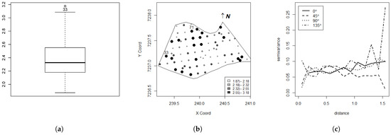
Figure 1. Boxplot (a), post-plot (b) and directional semivariogram (c) for the soybean productivity data set (t ha⁻¹).

Three outliers were observed in the boxplots of the explanatory variables. For the variable P, these were the observations $\#62$, $\#68$ and $\#69$ with respective values of $50.3$, $52.5$ and $58.6$ mg dm⁻³. For the variable pH, the graph highlighted the observations $\#56$, $\#55$, $\#14$, and $\#4$ with respective values of $5.8$, $6.0$, $6.0$, and $6.1$, and for the variable OM, only one outlier was detected—observation $\#71$ with $63.37$ g dm⁻³. The analysis of the directional semivariogram, given in Figure 1c for directions 0°, 45°, 90°, and 135°, indicates that it is reasonable to assume isotropy, since the spatial dependence structure is similar in the constructed directions.

Table 2 presents the parameter estimates for the reparameterized t-Student linear model considering different values for the parameter $\eta$ and different values of $\kappa$ for the Matérn family of geostatistical models and asymptotic standard errors (in parentheses). The parameter ${\varphi }_3$ was fixed at $0.3$, as obtained from a previous analysis using the ordinary least squares method.

Table 2. Parameters estimates and asymptotic standard errors in parenthesis.

$\mathit{\kappa }$	$\mathit{\eta }$	${\widehat{\mathit{\beta }}}_1$	${\widehat{\mathit{\beta }}}_2$	${\widehat{\mathit{\beta }}}_3$	${\widehat{\mathit{\beta }}}_4$	${\widehat{\mathit{\beta }}}_5$	${\widehat{\mathit{\varphi }}}_1$	${\widehat{\mathit{\varphi }}}_2$
0.5	$0.05$	$1.9712$	$0.0030$	$-0.0997$	$0.0379$	$0.0040$	$0.0330$	$0.0482$
		$\left(0.4227\right)$	$\left(0.0028\right)$	$\left(0.2269\right)$	$\left(0.0752\right)$	$\left(0.0055\right)$	$\left(0.0428\right)$	$\left(0.0491\right)$
	$0.10$	$1.9712$	$0.0030$	$-0.0997$	$0.0379$	$0.0040$	$0.0368$	$0.0540$
		$\left(0.4217\right)$	$\left(0.0028\right)$	$\left(0.2263\right)$	$\left(0.0750\right)$	$\left(0.0054\right)$	$\left(0.0493\right)$	$\left(0.0576\right)$
	$0.25$	$1.9712$	$0.0030$	$-0.0997$	$0.0379$	$0.0040$	$0.0585$	$0.0857$
		$\left(0.4205\right)$	$\left(0.0028\right)$	$\left(0.2257\right)$	$\left(0.0748\right)$	$\left(0.0054\right)$	$\left(0.0849\right)$	$\left(0.1032\right)$
	$0.45$	$1.9712$	$0.0030$	$-0.0997$	$0.0379$	$0.0040$	$0.2960$	$0.4336$
		$\left(0.4231\right)$	$\left(0.0029\right)$	$\left(0.2271\right)$	$\left(0.0753\right)$	$\left(0.0055\right)$	$\left(0.4693\right)$	$\left(0.5915\right)$
1.0	$0.05$	$2.0125$	$0.0037$	$-0.1263$	$0.0425$	$0.0025$	$0.1362$	$0.0113$
		$\left(0.5684\right)$	$\left(0.0039\right)$	$\left(0.3156\right)$	$\left(0.1043\right)$	$\left(0.0073\right)$	$\left(0.0971\right)$	$\left(0.0847\right)$
	$0.10$	$2.0125$	$0.0037$	$-0.1263$	$0.0425$	$0.0025$	$0.2102$	$0.0174$
		$\left(0.6664\right)$	$\left(0.0046\right)$	$\left(0.3700\right)$	$\left(0.1223\right)$	$\left(0.0085\right)$	$\left(0.1644\right)$	$\left(0.1309\right)$
	$0.25$	$2.0125$	$0.0037$	$-0.1263$	$0.0425$	$0.0025$	$0.6101$	$0.0504$
		$\left(0.8984\right)$	$\left(0.0062\right)$	$\left(0.4988\right)$	$\left(0.1649\right)$	$\left(0.0115\right)$	$\left(0.5852\right)$	$\left(0.3813\right)$
	$0.45$	$2.0125$	$0.0037$	$-0.1263$	$0.0425$	$0.0025$	$4.8771$	$0.4032$
		$\left(1.1362\right)$	$\left(0.0078\right)$	$\left(0.6308\right)$	$\left(0.2085\right)$	$\left(0.0146\right)$	$\left(5.6256\right)$	$\left(3.0600\right)$
1.5	$0.05$	$2.0118$	$0.0037$	$-0.1258$	$0.0425$	$0.0025$	$0.3658$	$0.1284$
		$\left(1.0406\right)$	$\left(0.0072\right)$	$\left(0.5774\right)$	$\left(0.1909\right)$	$\left(0.0133\right)$	$\left(0.8091\right)$	$\left(0.8023\right)$
	$0.10$	$2.0118$	$0.0037$	$-0.1258$	$0.0425$	$0.0025$	$0.6869$	$0.2411$
		$\left(1.3459\right)$	$\left(0.0093\right)$	$\left(0.7468\right)$	$\left(0.2469\right)$	$\left(0.0173\right)$	$\left(1.5368\right)$	$\left(1.5100\right)$
	$0.25$	$2.0118$	$0.0037$	$-0.1258$	$0.0425$	$0.0025$	$2.4208$	$0.8496$
		$\left(1.9992\right)$	$\left(0.0137\right)$	$\left(1.1093\right)$	$\left(0.3667\right)$	$\left(0.0256\right)$	$\left(5.5842\right)$	$\left(5.3471\right)$
	$0.45$	$2.0118$	$0.0037$	$-0.1258$	$0.0425$	$0.0025$	$20.9157$	$7.3408$
		$\left(2.6287\right)$	$\left(0.0181\right)$	$\left(1.4586\right)$	$\left(0.4822\right)$	$\left(0.0337\right)$	$\left(50.0842\right)$	$\left(46.4495\right)$

$\kappa$: kappa value of the Matérn model; $\eta$: parameter of form in the reparameterized t-Student distribution; ${\widehat{\beta }}_j$: parameters estimates, ${\widehat{\varphi }}_i$: parameters estimates of the covariance matrix, $i=1,2$, $j=1,2,3,4,5$, where ${\varphi }_1={\tau }_1$ and ${\varphi }_2={\tau }_2/{\tau }_3^{2\kappa }$, where ${\tau }_1$ is effect nugget and ${\tau }_2$ the contribution.

The chosen model is $\widehat{P}rod\left({\mathbf{s}}_i\right)=1.9712+0.0030\mathrm{P}\left({\mathbf{s}}_i\right)-0.0997\mathrm{K}\left({\mathbf{s}}_i\right)+0.0379\mathrm{pH}\left({\mathbf{s}}_i\right)+0.0040\mathrm{OM}\left({\mathbf{s}}_i\right)$, with an estimated covariance matrix given by $\widehat{\mathbf{\Sigma }}=0.0585{\mathit{I}}_{78}+0.0857\mathit{R}\left(0.3\right)$, where the elements of the correlation matrix $\mathit{R}$ determined from the Matérn family of models with $\kappa =0.5$ and $\eta =0.25$ were selected according to the cross-validation criterion ($CV$) and the trace ($T_r$) of the criteria of the asymptotic covariance matrix.

In the diagnostic analysis of the response variable, shown in Figure 2 and Figure 3, observations $\#17$, $\#18$, $\#33$, $\#70$, $\#71$, $\#72$, $\#76$ and $\#78$ are highlighted as influential points by Cook’s $D_i$ distance, and observations $\#18$, $\#46$, $\#70$, $\#76$, and $\#78$ are highlighted as influential points by the $Q{D}_i$ distance of the Q-function.

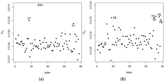
Figure 2. Global influence diagnostic plots $D{i}_{\beta }$ (a) and $D{i}_{\varphi }$ (b).

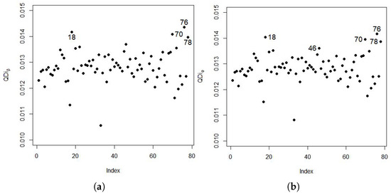
Figure 3. Global influence diagnostics plots $QD{i}_{\beta }$ (a) and $QD{i}_{\varphi }$ (b).

Figure 4 and Figure 5 show the local influence graphs; observations $\#33$ and $\#71$ were considered influential points for plot $C_i$ vs. index, $\left|Lmax\right|$ vs. index, and $\left|Qmax\right|$ vs. index. However, observations $\#4$, $\#14$, $\#62$, and $\#68$ are considered influential by the plot $C_{Qi}$. Observation $\#33$ is the same as the one detected in Figure 1a in the boxplot.

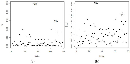
Figure 4. Local influence diagnostic plots $Ci$ (a) and $\left|lmax\right|$ (b).

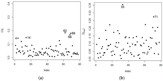
Figure 5. Local influence diagnostic plots $CQi$ (a) and $\left|Q_{max}\right|$ (b).

Figure 6 presents the graphs for the generalized leverage, which detected observations that had also been detected in the boxplots of the explanatory variables. The observations are $\#62,\#68$ and $\#69$ for P, $\#4,\#14,\#55$ and $\#56$ for pH and $\#71$ for OM.

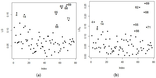
Figure 6. Generalized leverage plots considering the (a) log-likelihood function (LG) and (b) the Q-function $\left(L{G}_Q\right)$.

Figure 7 presents the QQ-plots of the residuals. It can be observed that when observation $\#33$ is removed, a better fit is detected at the top of the QQ-plot (Figure 7b), with most of the points closest to the line and all points belonging to the confidence interval in both graphs, showing that the data follow the assumed distribution.

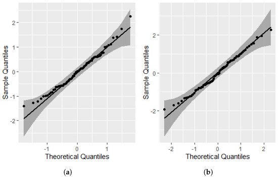
Figure 7. QQ-plots of the residuals (a) with all points and (b) without point #33.

Figure 8 presents the maps of predicted values considering all observations and deleting observation #33, which is evident in the substantial change on the map where observation #33 is located, see also Figure 1b. Thus, this observation is an outlier and an influential observation in obtaining the predicted values.

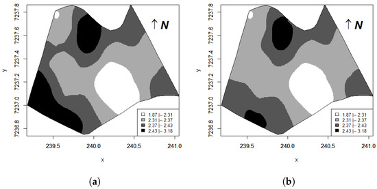
Figure 8. Maps for the data set (a) with all observations and (b) deleting observation #33.

To measure the similarity between the reference map (all points) and the model map (without point #33), global accuracy, the Kappa, and Tau were determined with AG = 0.73, T = 0.64 and Kp = 0.59, suggesting a difference between thematic maps [40,41].

4. Discussion

To explain the average soybean productivity, a multiple spatial linear regression model was constructed, considering as explanatory variables the chemical contents of the soil, P, K, pH, and OM, with spatially correlated errors. The parameters estimated by maximum likelihood are presented in Table 2, where the best model chosen for the spatial dependence structure, considering CV criteria and the trait (Tr), was the Matérn model with the shape parameters $\kappa =0.5$ (exponential model) and the shape parameter of the reparameterized t-Student distribution with $\eta =0.25$.

Point $\#33$, considered an outlier (Figure 1), was globally and locally influential (Figure 2, Figure 4 and Figure 5) when removed showing that the QQ-plot of the residues (Figure 7) has a better behavior, indicating that this observation is also an influential point in the probability distribution of the residues, as [5] values that deviate considerably from the straight line indicate influential cases.

When comparing the map generated with all sample points and the map without points $\#33$ (Figure 8), it can be seen that the global accuracy indicator (AG) is less than 0.73, indicating that the maps are dissimilar [40]. According to the classification of similarity indices, Tau ($T=0.64$) and Kappa ($Kp=0.59$) indicate that the maps have low similarity [40,41]. Thus, it is possible to verify that there is a difference in the classification of the constructed thematic maps with and without a point $\#33$ and with a point $\#33$ detected as influential in the elaboration of the map. The formulas for the indices $AG$, T, and $Kp$ are presented by [42].

The graphs of the generalized leverage indices LG and LG_Q (Figure 6 detected leverage points, indicating the existence of influential points in the explanatory variables and in the spatial linear regression model, affecting the estimates of the model parameters. Figure 6 detected observations $\#62$, $\#68$, and $\#69$ for phosphorus (P); observations $\#4$, $\#14$, $\#55$, and $\#56$ for hydrogen potential (pH); and observation $\#71$ for organic matter (OM), with potassium (K) not being a leverage point.

With information from the productivity map and explanatory variables, differentiated management units (DMUs) can be created, detecting subareas in the agricultural property under study that have similar characteristics in terms of production potential, helping the farmer apply differentiated management strategies for each subarea.

5. Conclusions

The reparameterized t-Student distribution was presented in the geostatistical framework. The reparametrization enables a straightforward comparison between the covariance matrix of multivariate distributions, especially for comparison with the multivariate normal distributions. The study also used global and local influence diagnostics to choose a more appropriate model to fit the data.

The reparametrized t-Student linear spatial modeling allows for more robust modeling in the presence of influential observations. It is extremely important to detect the influential points and correlate their spatial location, in order to draaw valuable conclusions about whether to remove these points or not, defined by the analysis of diagnostics. Investigation of theses points is indispensable for making a decision, ensuring that the information contained in the created maps is more consistent with reality and may be used in precision agriculture for the creation of differentiated management units.

References

- Galea, M.; Bolfarine, H.; Vilcalabra, F. Influence diagnostics for the structural errors-in-variables model under the Student-t distribution. J. Appl. Stat. 2002, 29, 1191–1204. [Google Scholar] [CrossRef]
- Galea, M.; de Castro, M. Robust inference in a linear functional model with replications using the t distribution. J. Multivar. Anal. 2017, 160, 134–145. [Google Scholar] [CrossRef]
- Martínez, S.; Giraldo, R.; Leiva, V. Birnbaum–Saunders functional regression models for spatial data. Stoch. Environ. Res. Risk Assess. 2019, 33, 1765–1780. [Google Scholar] [CrossRef]
- Ordoñez, J.A.; Prates, M.O.; Matos, L.A.; Lachos, V.H. Objective Bayesian analysis for spatial Student-t regression models. J. Spat. Sci. 2020. [Google Scholar] [CrossRef]
- Lange, K.L.; Little, R.J.A.; Taylor, J.M.G. Robust statistical modeling using the t distribution. JASA 1989, 84, 881–896. [Google Scholar] [CrossRef]
- Uribe-Opazo, M.A.; De Bastiani, F.; Galea, M.; Schemmer, R.C.; Assumpção, R.A.B. Appropriate perturbation scheme for the covariance matrix of a t-Student spatial linear model. Spat. Stat. 2021, 41, 100481. [Google Scholar] [CrossRef]
- Richetti, J.; Uribe-Opazo, M.A.; De Bastiani, F.; Johann, J.S. Techniques for detection of influencing points in regionalized continuous variables. Eng. Agríc. 2016, 36, 152–165. [Google Scholar] [CrossRef]
- Osorio, F.; Paula, G.A.; Galea, M. Assessment of local influence in elliptical linear models with longitudinal structure. Comput. Stat. Data Anal. 2007, 51, 4354–4368. [Google Scholar] [CrossRef]
- Uribe-Opazo, M.A.; Borssoi, J.A.; Galea, M. Influence diagnostics in Gaussian spatial linear models. J. Appl. Stat. 2012, 39, 615–630. [Google Scholar] [CrossRef]
- De Bastiani, F.; Galea, M.; Cysneiros, A.H.M.A.; Uribe-Opazo, M.A. Gaussian spatial linear models with repetitions: An application to soybean productivity. Spat. Stat. 2017, 21, 319–335. [Google Scholar] [CrossRef]
- De Bastiani, F.; Uribe-Opazo, M.A.; Galea, M.; Cysneiros, A.H.M.A. Case-deletion diagnostics for spatial linear mixed models. Spat. Stat. 2018, 28, 284–303. [Google Scholar] [CrossRef]
- Lachos, V.H.; Matos, L.A.; Barbosa, T.S.; Garay, A.M.; Dey, D.K. Influence diagnostics in spatial models with censored response. Environmetrics 2017, 28, e2464. [Google Scholar] [CrossRef]
- Zhu, H.; Lee, S.; Wei, B.; Zhou, J. Case-Deletion Measures for Models with Incomplete Data. Biometrika 2001, 88, 727–737. [Google Scholar] [CrossRef]
- Osorio, F. MVT: Estimation and Testing for the Multivariate t-Distribution. R Package Version 0.3-8. 2023. Available online: https://CRAN.R-project.org/package=MVT (accessed on 1 August 2024).
- Mardia, K.V.; Marshall, R.J. Maximum likelihood estimation of models for residual covariance in spatial regression. Biometrika 1984, 71, 135–146. [Google Scholar] [CrossRef]
- Stein, M.L. Interpolation of Spatial Data: Some Theory for Kriging; Springer Science & Business Media: Berlin/Heidelberg, Germany, 2012; pp. 1–249. [Google Scholar]
- Acosta, J.; Osorio, F.; Vallejos, R. Effective sample size for line transect sampling models with an application to marine macroalgae. J. Agric. Biol. Environ. Stat. 2016, 21, 407–425. [Google Scholar] [CrossRef]
- Waller, L.A.; Gotway, C.A. Applied Spatial Statistics for Public Health Data; John Wiley & Sons: Hoboken, NJ, USA, 2004; p. 368. [Google Scholar]
- Magnus, J.R.; Neudecker, H. Matrix Differential Calculus with Applications in Statistics and Econometrics; John Wiley & Sons: Hoboken, NJ, USA, 2019; p. 479. [Google Scholar]
- Zellner, A. Bayesian and non-Bayesian analysis of the regression model with multivariate Student-t error terms. JASA 1976, 71, 400–405. [Google Scholar] [CrossRef]
- De Bastiani, F.; Cysneiros, A.H.L.A.; Uribe-Opazo, M.A.; Galea, M. Influence diagnostics in elliptical spatial linear models. Test 2015, 4, 322–340. [Google Scholar] [CrossRef]
- Kano, Y.; Berkane, M.A.; Bentler, M. Statistical inference based on pseudo-maximum likelihood estimators in elliptical populations. JASA 1993, 88, 135–143. [Google Scholar]
- Matérn, B. Spatial Variation; Lecture Notes in Statistics; Springer: Berlin/Heidelberg, Germany, 1986; Volume 36. [Google Scholar]
- Dalposso, G.H.; Uribe-Opazo, M.A.; Johann, J.A.; Galea, M.; De Bastiani, F. Gaussian spatial linear model of soybean yield using bootstrap methods. Eng. Agríc. 2018, 38, 110–116. [Google Scholar] [CrossRef]
- Almeida, A.; Loy, A.; Hofnann, H. ggplo2 compatible quanttile-quantile plots in R. R J. 2018, 10, 248–261. [Google Scholar]
- Wickham, H. ggplot2. Wiley Interdiciplinary Rev. Stat. 2011, 3, 180–185. [Google Scholar] [CrossRef]
- Cook, R.D.; Weisberg, S. Residuals and Influence in Regression; Chapman and Hall: New York, NY, USA, 1982. [Google Scholar]
- Chatterjee, S.; Hadi, A.S. Sensitivity Analysis in Linear Regression; John Wiley & Sons: Hoboken, NJ, USA, 1986; p. 327. [Google Scholar]
- Christensen, R.; Johnson, W.; Pearson, L.M. Brediction diagnostics for spatial linear models. Biometrika 1992, 79, 583–591. [Google Scholar] [CrossRef]
- Pan, J.; Fei, Y.; Foster, P. Case-deletion diagnostics for linear mixed models. Technometrics 2014, 56, 269–281. [Google Scholar] [CrossRef][Green Version]
- Cook, R.D. Detection of influential observation in linear regression. Technometrics 1977, 19, 15–18. [Google Scholar] [CrossRef]
- Zhu, H.; Lee, S. Local influence for incomplete data models. J. R. Stat. Soc. B Stat. Methodol. 2001, 63, 11–126. [Google Scholar] [CrossRef]
- Cook, R.D. Assessment of local influence. J. R. Stat. Soc. B Methodol. 1986, 48, 133–155. [Google Scholar] [CrossRef]
- Zhu, H.; Ibrahim, J.G.; Lee, S.; Zhang, H. Perturbation selection and influence measures in local influence analysis. Ann. Stat. 2007, 35, 2565–2588. [Google Scholar] [CrossRef]
- Verbeke, G.; Molenberghs, G. Linear Mixed Models for Longitudinal Data; Springer Science & Business Media: Berlin/Heidelberg, Germany, 2009. [Google Scholar]
- Poon, W.Y.; Poon, Y.S. Conformal normal curvature and assessment of local influence. Stat. Methol. 1999, 61, 51–61. [Google Scholar] [CrossRef]
- Hoaglin, D.C.; Welsch, R.E. The hat matrix in regression and ANOVA. Ann. Stat. 1978, 32, 17–22. [Google Scholar] [CrossRef]
- St Laurent, R.T.; Cook, R.D. Leverage and superleverage in nonlinear regression. JASA 1992, 87, 985–990. [Google Scholar] [CrossRef]
- Wei, X.; Samarabandu, J.; Devdhar, R.S.; Siegel, A.J.; Acharya, R.; Berezney, R. Segregation of transcription and replication sites into higher order domains. Science 1998, 281, 1502–1505. [Google Scholar] [CrossRef] [PubMed]
- Anderson, J.R. A Land Use and Land Cover Classification System for Use with Remote Sensor Data; US Government Printing Office: Washinton, DC, USA, 1976; p. 964.
- Krippendorff, K. Content Analysis: An Introduction to Its Methodology; Sage Publications: Thousand Oaks, CA, USA, 1980. [Google Scholar]
- De Bastiani, F.; Uribe-Opazo, M.A.; Dalposso, G.H. Comparison of maps of spatial variability of soil resistance to penetration constructed with and without covariables using a spatial linear model. Eng. Agríc. 2012, 32, 393–404. [Google Scholar] [CrossRef]
Disclaimer/Publisher’s Note: The statements, opinions and data contained in all publications are solely those of the individual author(s) and contributor(s) and not of MDPI and/or the editor(s). MDPI and/or the editor(s) disclaim responsibility for any injury to people or property resulting from any ideas, methods, instructions or products referred to in the content. |
© 2025 by the authors. Licensee MDPI, Basel, Switzerland. This article is an open access article distributed under the terms and conditions of the Creative Commons Attribution (CC BY) license (https://creativecommons.org/licenses/by/4.0/).